the Creative Commons Attribution 4.0 License.
the Creative Commons Attribution 4.0 License.
 | 17 Apr 2019
Simple rules to minimise exposure to coseismic landslide hazard
David G. Milledge
Alexander L. Densmore
Dino Bellugi
Nick J. Rosser
Jack Watt
Katie J. Oven
Landslides constitute a hazard to life and infrastructure and their risk is mitigated primarily by reducing exposure. This requires information on landslide hazard on a scale that can enable informed decisions. Such information is often unavailable to, or not easily interpreted by, those who might need it most (e.g. householders, local governments and non-governmental organisations). To address this shortcoming, we develop simple rules to minimise exposure to coseismic landslide hazard that are understandable, communicable and memorable, and that require no prior knowledge, skills or equipment to apply. We examine rules based on two common metrics of landslide hazard, (1) local slope and (2) upslope contributing area as a proxy for hillslope location relative to rivers or ridge crests. In addition, we introduce and test two new metrics: the maximum angle to the skyline and the hazard area, defined as the upslope area with slope >40∘ from which landslide debris can reach a location without passing over a slope of <10∘. We then test the skill with which each metric can identify landslide hazard – defined as the probability of being hit by a landslide – using inventories of landslides triggered by six earthquakes that occurred between 1993 and 2015. We find that the maximum skyline angle and hazard area provide the most skilful predictions, and these results form the basis for two simple rules: “minimise your maximum angle to the skyline” and “avoid steep (>10∘) channels with many steep (>40∘) areas that are upslope”. Because local slope alone is also a skilful predictor of landslide hazard, we can formulate a third rule as “minimise the angle of the slope under your feet, especially on steep hillsides, but not at the expense of increasing skyline angle or hazard area”. In contrast, the upslope contributing area has a weaker and more complex relationship to hazard than the other predictors. Our simple rules complement but do not replace detailed site-specific investigation: they can be used for initial estimations of landslide hazard or to guide decision-making in the absence of any other information.
- Article
(14289 KB) - Full-text XML
-
Supplement
(2664 KB) - BibTeX
- EndNote


Landslides involve the downward movement of soil or rock under gravity, sometimes mixing with water or air to run out rapidly over long distances. Landslides have considerable destructive potential and constitute a major hazard to life and infrastructure (e.g. Froude and Petley, 2018).
Landslide risk can be mitigated by either reducing exposure – the likelihood that a particular person or structure is hit by a landslide – or by reducing the consequences of landslide impact. The latter is expensive for a building (Fell et al., 2005; Volkwein et al., 2011; Guillard-Gonçalves et al., 2016) and extremely difficult for a person (Kennedy et al., 2015). As a result, efforts in reducing landslide risk tend to focus on reducing exposure, primarily by siting infrastructure and assets (or by choosing to spend time) in places of lower landslide hazard. These choices, however, require information on landslide hazard on a scale that can enable informed decisions about how to mitigate the risk. In other words, a decision to reduce landslide exposure requires knowledge of how landslide hazard varies in space.
Quantitative landslide hazard information is commonly expressed as a relative weighting or probability of landslide occurrence in a given location and over a specified period of time. This is often communicated as a hazard map (Dransch et al., 2010). These maps can provide useful information to inform decisions such as siting infrastructure, allocating resources, designing countermeasures or planning mitigation measures such as evacuation routes. There are, however, at least five limitations to reliance on hazard maps as the sole source of landslide hazard information. First, landslide hazard maps do not exist for all hazardous locations, since their generation requires technical expertise and site-specific information (such as geological maps or landslide inventories) that may not be available. Second, where maps do exist they may not be available to those that need them. Whether in physical or digital form, hazard maps are rarely held by the communities that live within their boundaries (Alexander, 2005; Mills and Curtis, 2008; Twigg et al., 2017). Third, where landslide hazard maps are available, their resolution may not be fine enough to address the questions that potential users will have. In everyday decisions, from where to build a house to which way to walk, distances of even a few metres can matter greatly for determining landslide exposure, because landslide hazard can vary substantially even over such short distances. National- and even regional-scale hazard maps do not resolve hazard on those scales, however, and hazard maps on the appropriate scale would be extremely costly and time consuming to produce over large areas. Fourth, landslide hazard maps are designed for technical users (such as engineers and planners) and thus can be difficult for non-technical users to interpret (Dransch et al., 2010). Hazard is often expressed in probabilistic terms which are inherently difficult to communicate and understand (Thompson et al., 2015). The maps may also require particular equipment, such as a computer with appropriate software, or additional contextual information to enable clear visualisation or orient the user (Mills and Curtis, 2008). Finally, landslide hazard maps may lack the appropriate information for decision-making. For example, landslide hazard is commonly equated simply with the probability of landslide initiation at a given location, rather than the probability that the location will be impacted by a landslide occurring there or somewhere upslope.
In the absence of detailed hazard maps, how should we make decisions about siting infrastructure or spending time in landslide-prone areas? An alternative and complementary form of hazard information might be a set of general rules that can be memorised by anyone who might be exposed to landslide hazard, or by those charged with managing landslide risk, to be applied where no other information exists. A good general rule should (1) be understandable, communicable and memorable; (2) require no prior knowledge, skills or equipment to evaluate; (3) be a skilful discriminant of hazard; and (4) be cast so that it does not increase exposure to another hazard. A good example of such a rule would be the instruction to minimise exposure to tsunami: “in case of earthquake, go to high ground or inland” (Atwater et al., 1999, p. 20). Research has shown that these types of simple rules are already to some extent implicitly coded into the decisions that people make (e.g. Gigerenzer, 2008), reflecting tacit knowledge of hazard (e.g. Shaw et al., 2008; Twigg et al., 2017). Importantly, however, there are limits to this tacit knowledge (Briggs, 2005); in particular, the body of experience required to generate these rules is limited by both the infrequency of triggering events, such as earthquakes or large storms, and a focus on normal, rather than unusual, but not improbable events, which can introduce biases (McCammon, 2004; Kahneman and Klein, 2009). For example, while perennial rainfall-triggered landslides and the risks that they pose may be familiar to people in landslide-prone communities, landslides triggered by large earthquakes may fall outside residents' lived experiences and so will be more challenging to comprehend and account for in decision-making. If simple, memorable rules (fulfilling criteria one and two above) could be derived from a large inventory of hazardous events, these biases might be reduced while maintaining the other benefits of a rule-based approach (criteria three and four). Such a set of data-based rules could be used in the absence of, or in conjunction with, existing tools such as hazard maps and local knowledge, both to inform decisions and to inspire discussion amongst householders, local government and non-governmental organisations. Such knowledge is commonly in demand, not only from technical users but also from lay people (Twigg et al., 2017; Datta et al., 2018), especially because self-recovery after disasters (for example, via reconstruction programmes in which householders rebuild their own homes) is increasingly recognised as a critical mechanism of recovery (Twigg et al., 2017).
Here we focus on rules that can be derived from the topography surrounding a given location and that differentiate exposure to coseismic landslide hazard over distances of tens to hundreds of metres. Such rules are likely to be most useful for decisions made before an earthquake about where to site infrastructure or spend time, and may be less useful for decisions about where to go during an earthquake when time is limited. We focus on earthquakes because landsliding is an important but poorly understood aspect of hazard in many recent continental earthquakes (Huang and Fan, 2013; Roback et al., 2018). We consider the extent to which our results may be transferrable to landslides caused by more frequent triggers, such as storms, in the discussion.
We examine candidate rules based on our existing understanding of landslide mechanics to identify those that meet criteria one and two above. We then test the skill with which each candidate rule can identify landslide hazard, using inventories of coseismic landslides from the recent Finisterre (Papua New Guinea), Northridge (USA), Chi-Chi (Taiwan), Wenchuan (China), Haiti and Gorkha (Nepal) earthquakes. Our goal is to determine the rule or rules that best fulfil the four criteria listed above and that therefore provide the best combination of simplicity and skill in anticipating coseismic landslide impacts. We ask two key questions. (1) To what extent could observed landslide locations in past earthquakes have been predicted by these simple rules alone, without recourse to more complex models? (2) Is there a single rule or set of rules that performs well across all earthquakes and could form the basis for anticipating landslide-affected locations in a future earthquake? The first question relates to the absolute performance of the rule set, while the second relates to the relative performance of rules within the set. While spatial patterns of landsliding in these earthquakes have been previously established, this is to our knowledge the first attempt to extract a more general set of rules from landslide data sets across multiple earthquakes.
This paper is necessarily technical, addressing the question of whether it is possible to formulate such rules, identifying which rules work best and assessing their performance. We therefore expect the paper's primary audience to be technical experts with an interest in landslide risk reduction. We have begun to explore ways of expressing these rules in a format that is more accessible to a general audience (e.g. Milledge et al., 2018).
Local slope, the gradient of the ground surface measured over some short distance (usually ∼1–100 m), has been identified as an important driver of landslide occurrence in almost all prior landslide studies (e.g. Harp et al., 1981; Tibaldi et al., 1995; Keefer, 2000; Wang et al., 2003; Xu et al., 2012, 2014a; Parker et al., 2017). This is consistent with mechanistic expectations based on the balance of driving and resisting forces on an inclined failure plane (Taylor, 1937). Local slope is an intuitive parameter that is familiar to most people and can be easily estimated in relative terms (i.e. hillside A is steeper than hillside B) without specialised equipment. Seismic acceleration or shaking is commonly identified as the other dominant control on coseismic landslide occurrence (Khazai and Sitar, 2004; Meunier et al., 2007). However, shaking for any future earthquake cannot be predicted due to a lack of certainty on source location, magnitude, rupture style and local site effects (Geller, 1997). It is therefore difficult to incorporate it into a general rule for future landslide hazard.
Ridges are often considered to be areas of high coseismic landslide probability due to topographic amplification (Densmore and Hovius, 2000; Meunier et al., 2008; Rault et al., 2018), while rivers are by definition areas of flow concentration into which landslides from multiple potential initiation zones may run out. Here we use the upslope contributing area as a continuous estimator of the proximity to a ridgeline (defined here as an area with little or no upslope cells) or a valley in order to assess how hazard may vary with position in the landscape.
Other predictors have been identified in coseismic landslide studies, but these generally have a secondary effect and are not consistently identified as important controls on landslide occurrence (Parker et al., 2017). Elevation and aspect in particular lack a consistent explanation or pattern as a control on coseismic landslide hazard (Parker et al., 2017). Other common predictors are difficult to evaluate on the ground without specialised equipment or knowledge. Soil type (e.g. Lee and Pradhan, 2007), rock type (e.g. Parise and Jibson, 2000) or land cover (e.g. Pradhan, 2013) may be relevant to slope stability but are difficult to identify without specialised training. Curvature (e.g. Xu et al., 2014a) is strongly dependent on the length scale over which it is measured and is extremely difficult to estimate by eye, particularly in rough natural topography. Proximity to roads (e.g. Xu et al., 2012) is often possible to estimate in the field, but inclusion of this factor assumes that all roads are similar in their design, age and construction and thus have similar impacts on slope stability.
The potential predictors described above are primarily chosen in hazard models for their perceived link to the probability of coseismic landslide initiation. Once triggered, however, landslide material may run out for long distances and over large areas. Thus, there are substantial portions of any landscape where landslide initiation is unlikely but where contact with a landslide is still possible – for example, at the foot of a steep hillslope. Mechanistic modelling of landslide run-out is computationally intensive and strongly sensitive to initial conditions, taking it beyond the capacity of exposed communities (e.g. George and Iverson, 2014). In contrast, simple empirical approaches that have shown some predictive power fall into two categories: reach angles and run-out routing.
The Fahrboeschung or reach angle from the crown of a landslide to the toe of its deposit has been shown to follow an exponential decrease with landslide volume (Heim, 1832; Corominas, 1996; Hunter and Fell, 2003). The reach angle concept has been incorporated into a small number of hazard maps as a way to represent the probability that a landslide will reach a given location, which can then be coupled with predictions of the probability of landslide initiation (e.g. Kritikos et al., 2015). However, these complex combinations of probability are difficult to distil into a single simple rule and, to our knowledge, this has not yet been done.
If initiation probability is unknown and we make the conservative assumption that any cell can initiate a landslide, then the hazard at a given location becomes proportional to the area that protrudes above a cone with its apex at the location of interest and its sides inclined at a critical reach angle from the horizontal. This approach has similarities with local sloping base level (Jaboyedoff et al., 2004) and excess topography metrics (Blöthe et al., 2015), which both project surfaces through the landscape to identify less stable zones, though neither of these approaches is framed in terms of reach angles. Even this simple approach, which neglects initiation probability, is hard to distil: (1) its conceptual complexity makes it difficult to communicate, (2) its predictions depend on a reach angle parameter that is poorly constrained, and (3) the area protruding from an imaginary surface projected beneath the land surface is very difficult to estimate by eye, particularly in high-relief areas where significant parts of the landscape may be occluded from the viewpoint. An alternative metric would simply be the maximum angle from the horizontal to the skyline, which can be interpreted as the maximum (or worst-case) reach angle for that location. This metric is much simpler and thus easier to communicate and remember, can be estimated by eye and avoids the problem of choosing a critical reach angle. We choose this as our third potential hazard predictor.
Run-out routing approaches assess the probability that landslide debris will reach a given location by assuming that it flows downslope and that its probability of stopping is dependent on some local property of the path along which it flows. This approach ranges in complexity from detailed physics-based treatments (George and Iverson, 2014; von Ruette et al., 2016) to simple empirical rules such as the local slope or junction angle of flow paths (Benda and Cundy, 1990; Montgomery and Dietrich, 1994; Densmore et al., 1998; Fannin and Wise, 2001). Hazard estimates are then a function of the initiation probability integrated over the upslope area and the stopping probability for each potential event. To incorporate these considerations as simply as possible into a hazard predictor, we introduce a new approach (described below) that accounts for local slope both at the locations of landslide initiation and along the flow path. While this approach does not capture the dynamic behaviour of landslide initiation or run-out, we include it so that we can test the skill of such non-local approaches and the need to account for them in our simple rules.
In this section, we describe the landslide inventories against which we test our four potential predictors. A Mw 6.9 earthquake occurred on 13 October 1993 in the Finisterre Mountains of Papua New Guinea with a hypocentre at 25 km depth, rupturing the north-dipping Ramu–Markham thrust fault to within a few hundred metres of the surface (Stevens et al., 1998). The event was followed by multiple aftershocks of >Mw 6, including a Mw 6.7 event on 25 October 1993 with a hypocentre at a depth of 30 km. About 4700 landslides triggered by these earthquakes were mapped from 30 m resolution SPOT images (Meunier et al., 2007). Location accuracy for the landslides is thought to be similar to the pixel size of the satellite images used, ∼30 m.
The Mw 6.7 Northridge earthquake occurred in southern California, USA, on 17 January 1994 and ruptured 14 km of a south-dipping blind thrust fault, with a hypocentre at 19 km depth (Wald and Heaton, 1994; Hauksson et al., 1995). The earthquake triggered more than 11 000 landslides (Harp and Jibson, 1996). Landslides were mapped immediately after the earthquake using field studies and aerial reconnaissance and were manually digitised on 1:24 000 scale base maps. Landslides >10 m across could be confidently identified and location errors were estimated to be <30 m (Harp and Jibson, 1996).
The Mw 7.6 Chi-Chi earthquake occurred on 21 September 1999 with a hypocentre at 8–10 km depth, rupturing ∼100 km of the east-dipping Chelungpu thrust fault in western Taiwan (Shin and Teng, 2001). The earthquake triggered more than 20 000 landslides with the majority occurring across a 3000 km2 region (Dadson et al., 2003). Landslides in this region were mapped by the Taiwan National Science and Technology Center for Disaster Prevention from SPOT satellite images with a resolution of 20 m. Landslides with areas >3600 m2 were resolved, resulting in an inventory of 9272 landslides with location errors estimated to be ∼20 m (Dadson et al., 2004).
The Mw 7.9 Wenchuan earthquake occurred on 12 May 2008 with a hypocentre at 14–19 km depth, rupturing ∼320 km of the steeply northwest-dipping Yingxiu–Beichuan and Pengguan faults in Sichuan, China (Xu et al., 2009). The earthquake triggered more than 60 000 landslides across a total area of 35 000 km2 (Gorum et al., 2011; Li et al., 2014). We used a subset of the landslide inventory compiled by Li et al. (2014), who mapped landslides from high-resolution (<15 m) satellite images and air photos. The subset of 18 700 landslides comprises all mapped landslides east of 104∘ E (Fig. S6 in the Supplement) and was chosen to avoid gaps in the available 30 m resolution SRTM topographic data. The subset covers a similar range of topographic and lithologic conditions and experienced a similar range of peak ground accelerations (0.16–1.3 g) to the full inventory (0.12–1.3 g). Location accuracy for landslides is thought to be similar to the pixel size of the satellite images used, ∼15 m (Li et al., 2014).
The Mw 7.0 Haiti earthquake occurred on 12 January 2010, with a hypocentre at 13 km depth (Mercier de Lépinay et al., 2011). The complex rupture involved both a blind thrust fault and deep lateral slip on the Enriquillo–Plantain Garden fault (Hayes et al., 2010; Mercier de Lépinay et al., 2011). The earthquake triggered more than 30 000 landslides across a 3000 km2 region (Xu et al., 2014a). We used an inventory of 23 679 landslides mapped by Harp et al. (2016) from publicly available satellite imagery with a resolution of 0.6 m before and after the earthquake; landslides with areas >10 m2 were resolved (Harp et al., 2017).
The Mw 7.8 Gorkha earthquake occurred on 25 April 2015, rupturing ∼140 km of the north-dipping Main Himalayan Thrust in central Nepal (Hayes et al., 2015; Elliott et al., 2016). It had a hypocentre at 8.2 km depth but did not rupture to the surface (Hayes et al., 2015). The event was followed by a series of large aftershocks, including a Mw 7.2 event on 12 May, which ruptured a portion of the Main Himalayan Thrust directly east of the 25 April rupture (Avouac et al., 2015). The earthquake triggered approximately 25 000 landslides with a total surface area of about 87 km2 (Roback et al., 2018). We used an inventory of 24 915 landslides mapped by Roback et al. (2018) from Worldview-2, Worldview-3 and Pleiades imagery, with a resolution of 0.25–0.5 m, before and after the earthquake.
These epicentral areas encompass a large range of millennial-scale erosion rates (0.1 to >7 mm yr−1), lithological properties (metamorphic, igneous and sedimentary), climatic conditions (Mediterranean to tropical) and vegetation covers (chapral, savannah, tundra, tropical and subtropical forest); see Table S2 and Figs. S3–S8 in the Supplement. We choose this range of settings in order to test the general applicability of any rules that we can extract.
5.1 Conditional probability and landslide hazard
Landslide hazard can be defined as the probability of being hit by a landslide in a given location and within a given time interval (Lee and Jones, 2004). Here we make no distinction between the consequences of being hit by landslides of different sizes or velocities, assuming that all are equally dangerous. This probability can be expressed mathematically as , where L is the outcome of being hit by a landslide, x,y are the coordinates for a particular location, and t is the time interval of interest. We do not address the timing of landsliding, assuming that this is driven by the timing of an earthquake and is thus unpredictable (Geller, 1997). Instead we focus on landslide susceptibility given an earthquake that produces shaking of unknown intensity at a location (x,y), hence the notation . We assume that the hazard at that location can be approximated by some location-specific characteristic (a). Thus, the landslide hazard at (x,y) is the conditional probability of being touched by a landslide given the value of the characteristic at that location, P(L|a), and can be calculated using Bayes' theorem:
where a is a specific characteristic of the location, such as the topographic slope. If we assume that the relationships between past landslides and local characteristics are good predictors of their future relationships then we can construct empirical conditional probability calculations from landslide inventories. This approach has proved successful for a range of applications, including identifying topographic controls on vegetation patterns (Milledge et al., 2012) and the rainfall conditions that trigger landslides (Berti et al., 2012). If we grid the topography, then the Bayes equation can be easily rewritten in terms of numbers of grid cells, and in this form the direct equivalence of landslide conditional probability and landslide area density (e.g. Meunier et al., 2007; Dai et al., 2011; Gorum et al., 2014) is clear:
where N(a∩L) is the number of cells with a given value of characteristic a that are touched by a mapped landslide, N(a) is the number of cells with the characteristic of a in the entire study area, and the study area is defined by the smallest convex hull that contains all of the observed landslides. To account for variability in the magnitude of shaking between the six study areas, we normalise the conditional probability of being hit by a landslide P(L|a) by the study area average probability of landsliding P(L) to generate a relative hazard. This can be shown to be directly equivalent to the frequency ratio (e.g. Lee and Pradhan, 2007; Lee and Sambath, 2006; Yilmaz, 2009; Kritikos et al., 2015):
where N(S) is the total number of cells in the study area and N(L) is the number of cells touched by landslides. Our normalised conditional probability is also directly equivalent to the probability ratio used by Lin et al. (2008) and Meunier et al. (2008) since, from Bayes' theorem:
We display the normalised conditional probability on a logarithmic scale for readability, resulting in a probability metric that is strongly similar to the information value metric used in some landslide susceptibility analyses (e.g. Yin and Yan, 1988). We evaluate both one-dimensional conditional probability in terms of one predictor variable and two-dimensional conditional probability in terms of two predictors considered jointly.
Conditional probability analysis is advantageous for its direct link to hazard and does not require us to impose a functional form to the data. However, the results are partly dependent on bin size and location for the predictor variable, and bins with few observations (i.e. those for which N(a)≪N(S)) can result in noisy data that are difficult to interpret. We use the approach by Rault et al. (2018) to identify the parts of the conditional probability data where our observations are sparse, leading to lower confidence in the results. We compute the confidence interval Ip associated with the random drawing of the N(L) landslide cells from the landscape distribution of the predictor variable. If the normalised conditional probability is within the interval Ip then we cannot exclude the possibility that the difference between the conditional and study area average probabilities is simply the result of random fluctuations. Given that landslides are rare events, even in these large earthquakes, we assume that landslides are independent and can be modelled with Bernoulli sampling. Since the binomial distribution is well approximated by a normal distribution when samples sizes are large (i.e. N(L)>30) and in the absence of extreme skew (i.e. and , then the 90 % confidence interval can be estimated as follows:
We distinguish conditional probability values that exceed this confidence interval Ip in the analysis below.
To aid interpretation in the two-dimensional case, we also perform a two-variable logistic regression with both local slope and upslope contributing area as predictors. While other statistical approaches could be used here (e.g. Pradhan, 2013), our intention is not to find the statistical approach that provides the most powerful synthesis of the different variables but to test the effectiveness of the variables themselves at distinguishing hazard when applied in the form of simple rules.
5.2 Receiver operating characteristic curves
Any simple rule for identifying more or less hazardous locations in the landscape will produce a relative measure of landslide probability. To evaluate this measure against a binary landslide map or inventory (where every cell is classified as landslide or non-landslide), it must be converted into a binary classification. A common approach to this problem is to construct a receiver operating characteristic (ROC) curve (e.g. Frattini et al., 2010). This curve quantifies both the benefit of a given classification in terms of successfully classified outcomes (landslide and non-landslide locations correctly identified, representing true positive and true negative outcomes respectively) and also the cost (non-landslides identified as landslides, known as false positives, and the opposite, known as false negatives). The ROC curve is constructed by thresholding a continuous variable (e.g. slope) and calculating the true positive rate as the number of true positives normalised by all positive observations and the false positive rate as the number of false positives normalised by all negative observations. Evaluation of these rates at different threshold values results in a curve, where the 1:1 line reflects the naïve random case. The area under the curve (AUC) tends to 1 as the skill of the classifier improves towards perfect classification and to 0.5 as the classifier worsens towards the naïve case. We calculate ROC curves for all of our chosen predictive approaches for each inventory.
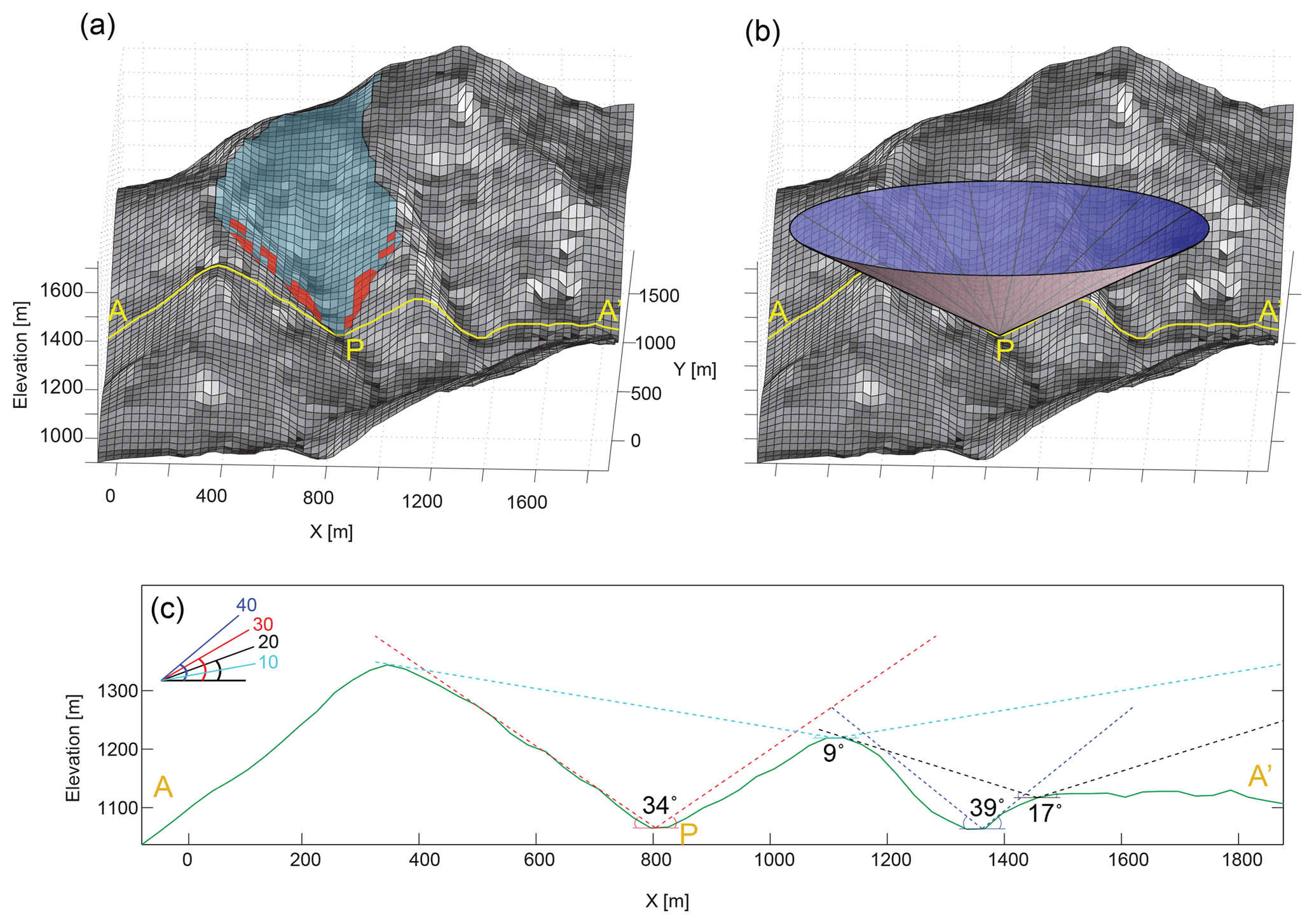
Figure 1Schematic view of the different topographic metrics tested here. (a) Perspective view of a landscape with each cell shaded according to its local slope from light (steep) to dark (gentle). The upslope contributing area for point P is coloured blue, and the cells steeper than 40∘ that have a flow path to P that is never less than 10∘ are coloured red. (b) The same perspective view with a cone projected from point P at an angle of 34∘ so that the surface of the cone is in places tangent to but never intersects the ground surface, indicating a maximum skyline angle of 34∘ for point P. (c) Cross section A–A' through the landscape (highlighted in yellow on a and b) with dashed lines showing skyline angles at four example locations.
5.3 Topographic analysis
All of the metrics tested here are defined using topographic data in the form of digital elevation models (DEMs). We use 30 m resolution DEM data drawn from the most widely used, freely available source for each site: for Northridge they are derived from downsampled 10 m NED elevation data (https://ned.usgs.gov/, last access: 29 March 2019), while for all other sites we use 1 arcsec Shuttle Radar Topography Mission (SRTM) elevation data (http://srtm.csi.cgiar.org/, last access: 29 March 2019).
5.3.1 Slope and upslope contributing area
We calculate local slope as the steepest path to a downslope neighbour from each cell (Travis et al., 1975) because calculating slope over larger (e.g. 3×3 cell) windows for a 30 m resolution DEM results in considerable underestimation (Claessens et al., 2005). We calculate the upslope contributing area using a multiple flow direction algorithm (Quinn et al., 1991) having filled pits using a flood fill algorithm (Schwanghart and Kuhn, 2010) and normalising by the grid cell width to minimise grid resolution biases. These topographic analyses are performed in Matlab using TopoToolbox v1.06 (Schwanghart and Kuhn, 2010).
5.3.2 Skyline angle analysis
To capture the effects of both landslide initiation and run-out, we define the skyline angle as the maximum angle from horizontal to the skyline for a given location (Fig. 1b and c). This metric is easily estimated by eye in the field and gives a worst-case reach angle for the location of interest but is run-out-dominated in that it does not take into account the probability of initiation.
For each cell in a study area, we estimate the skyline angle by calculating vertical angles between the target cell and every other cell within a 4.5 km radius. This search radius is chosen to greatly exceed the average hillslope lengths in all study areas and thus to fully capture the local skyline. The longest average hillslope length out of our study areas is ∼500 m for Wenchuan, estimated following the method of Roering et al. (2007). We choose a search radius 9 times larger than this hillslope length to ensure redundancy in capturing the local skyline and because the only disadvantage of a larger radius is increased computational cost. This approach is physically limited in at least two ways (Fig. 1a). First, it does not account for the dependence of run-out on the size of the initial failure or on increases or decreases of failure volume during run-out (e.g. Corominas, 1996). Second, it does not honour potential material flow paths. That is, the skyline cell that generates the steepest slope to the target cell may not be connected to the target cell by a flow path with monotonically decreasing elevation. However, this metric provides a measure of the gravitational potential energy available to drive run-out in the vicinity of the target cell.
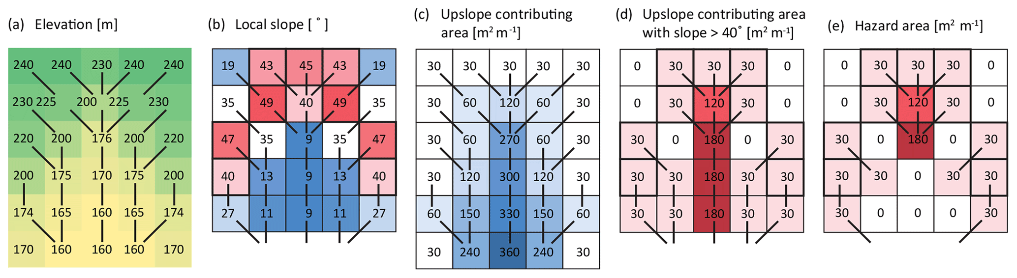
Figure 2SHALRUN-EQ hazard area calculations for a simplified (steepest flow path) example with an initiation angle of 40∘ and a stopping angle of 10∘: (a) elevations from a 30 m resolution digital elevation model for an area of topographic convergence, where lines show flow paths from cell to cell; (b) local slope with thick outlines showing cells steeper than 40∘; (c) upslope contributing area; (d) upslope contributing area steeper than 40∘; and (e) hazard area, i.e. the upslope area steeper than 40∘ with flow paths that do not fall below 10∘.
5.3.3 Run-out routing analysis
To assess the importance of non-local run-out paths on landslide probability, we follow the approach by Dietrich and Sitar (1997), who proposed the simplest possible debris flow run-out model, requiring only thresholds to define the initial instability and for downslope motion to continue. This simple model, referred to as SHALRUN, has been integrated with the coupled hydrologic-slope stability model SHALSTAB in an efficient parallel framework to predict landslide hazard potential in California (Bellugi et al, 2011). SHALRUN requires only two field-calibrated parameters: a critical rainfall threshold to define instability and a minimum slope threshold for downslope motion to continue. To apply this model in the context of coseismic landslides, we modify the condition for landslide initiation by replacing the critical rainfall threshold with a slope threshold to create a new model that we refer to as SHALRUN-EQ. We thus assume that landslide initiation and deposition are entirely dependent on the local slope of the ground surface – that is, landslides are more likely to initiate on steeper slopes and deposit on flatter slopes. More formally, SHALRUN-EQ predicts the upslope hazard area Ah as the upslope area weighted by the joint probability of landslide initiation and run-out (Figs. 1a and 2). Locations with higher Ah should have higher exposure to coseismic landslide hazard than those with low (or no) Ah. Formulation of the model requires (1) determination of the mobilisation probability at each cell i in the study area, (2) determination of the connection probability for mobilised material from each cell i to the target cell j, (3) convolution of (1) and (2) to get the locational hazard and (4) accumulation of the locational hazard to determine a hazard area above each target cell j.
In order to generate a simple rule, our model assumes that landslide initiation and deposition are entirely dependent on the local slope of the ground surface θ. For landslide initiation, we assume that locations steeper than a threshold slope θm are all equally capable of initiating a landslide with probability :
where θi is the observed local slope in a downslope direction at cell i and θm is the threshold slope required for landslide initiation.
In order to represent a landslide hazard, mobilised material must be able to run out from the initiation point i to the target cell j. This relationship is binary: either these points are connected by a viable run-out path or they are not. We define flow paths using multiple flow routing to all downslope cells weighted by the slope of the flow path (Quinn et al., 1991). This path must enable continued run-out for its entire length; if at any point on the flow path the material is fully deposited, then that initiation zone will be disconnected from the target cell j. Surface slope has previously been used to describe the probability that landslide material entering a cell will be deposited rather than continuing into the next downslope cell (e.g. Benda and Cundy, 1990; Fannin and Wise, 2001). For landslide deposition, we apply the simplest possible stopping condition and assume that landslide run-out ceases on slopes gentler than a critical angle (θs). The probability that a landslide initiated at cell i reaches the target cell j () can thus be expressed as follows:
where θminij is the minimum slope along the flow path from cell i to cell j, and θs is the critical slope required for stopping. We recognise that this simple stopping condition would be violated for landslides large enough to continue beyond the first cell with angle below the deposition threshold and discuss the implications of this simplification in Sect. 7.1.
We combine the initiation and run-out probabilities to calculate the locational hazard as the area ai of cell i weighted by the probability that a landslide is both mobilised in cell i and is connected to cell j:
Assuming that θs>0, we calculate the hazard area for each target cell j by summing locational hazard in the n cells upslope of j, normalised by grid cell width to minimise grid resolution bias:
where lj, is the grid cell width (30 m). Equation (9) is evaluated for every cell in the study area to generate a spatial grid of hazard area Ah (Fig. 2). Our choice of step functions for the mobilisation () and connection (Pcj) probabilities allows us to interpret Ah as the upslope area with a slope steeper than θm from which landslide debris can reach the target cell without passing over a slope gentler than θs. Alternative formulations could be used for and Pcj but these would result in a less intuitive index that would be difficult to implement as a simple rule.
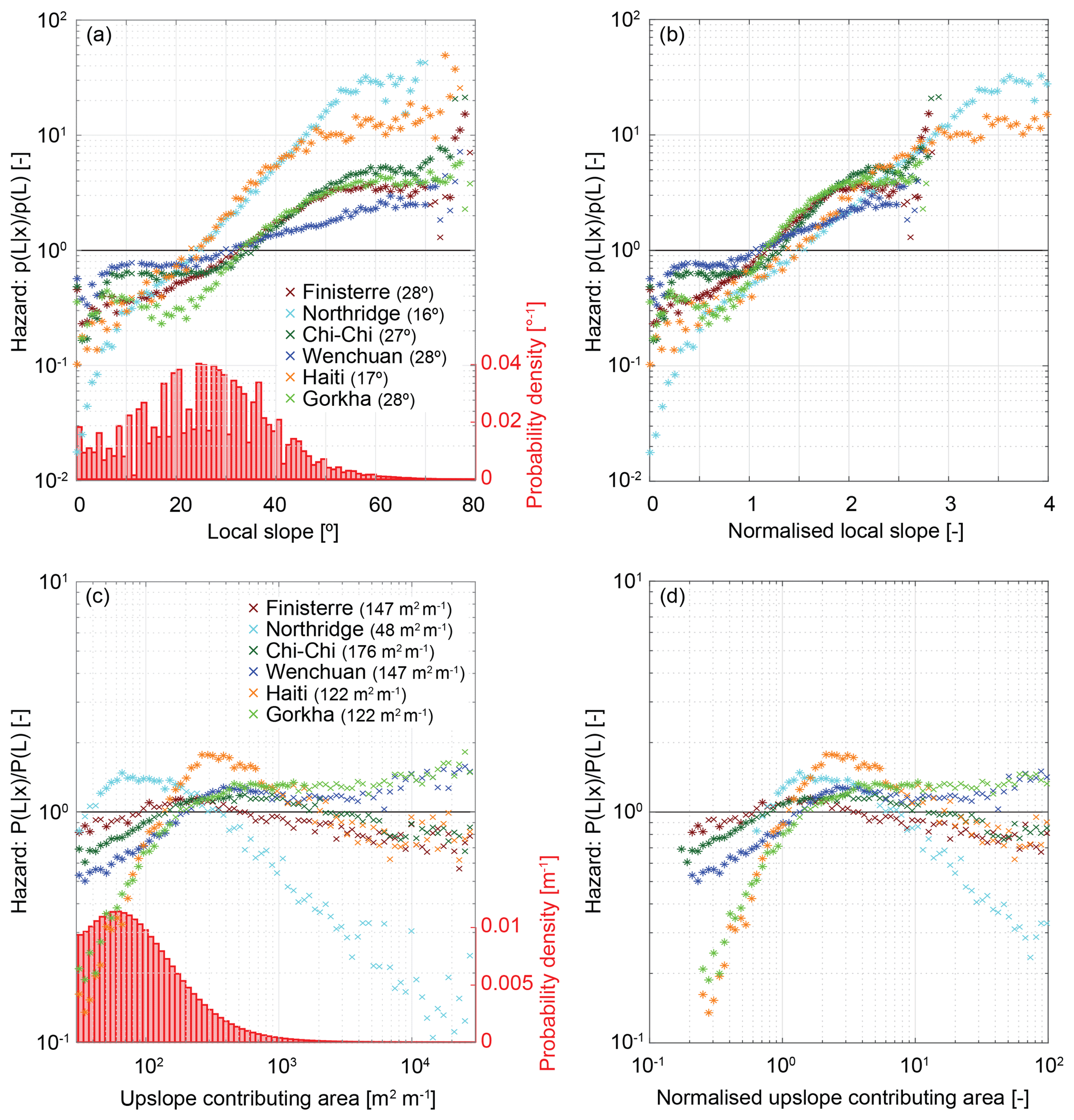
Figure 3Landslide hazard defined as conditional probability P(L|x) normalised by study area average landslide probability P(L), where x is (a) local slope; (b) local slope normalised by the study area average slope; (c) upslope contributing area per unit cell width; and (d) upslope contributing area normalised by the upslope contributing area of the inflection in average slope. Solid black lines show normalised probability of 1, the study area average; thus, points above this line have above-average landslide hazard compared to the study area as a whole. Asterisks indicate values for which conditional probability differs from the study area average probability at 90 % confidence. Red bars in (a) and (c) show histograms of local slope and upslope contributing area over the six inventories. Numbers in brackets show study area average slopes in (a) and upslope contributing area at the hillslope–channel transition in (c).
There is implicit resolution dependence to the stopping condition θs because it assumes that the low-gradient area is long enough (in terms of flow path length) that the landslide will stop. Similarly, there is resolution dependence to the initiating condition θm, as topographic surfaces will be more or less smooth, depending on the resolution of the DEM (Claessens et al., 2005). Also, the initiation probability is based on local slope alone and so does not account for any of the other possible drivers of coseismic landslide initiation, such as topographic amplification (Meunier et al., 2008) or pore water pressure (e.g. Xu et al., 2012). While many more complex models exist that account for initiation volumes and flow dynamics (e.g. George and Iverson, 2014; von Ruette et al., 2016), we seek the simplest possible model that captures the effects of drainage networks in accumulating hazard, of steep slopes in landslide initiation and of gentle slopes in landslide deposition.
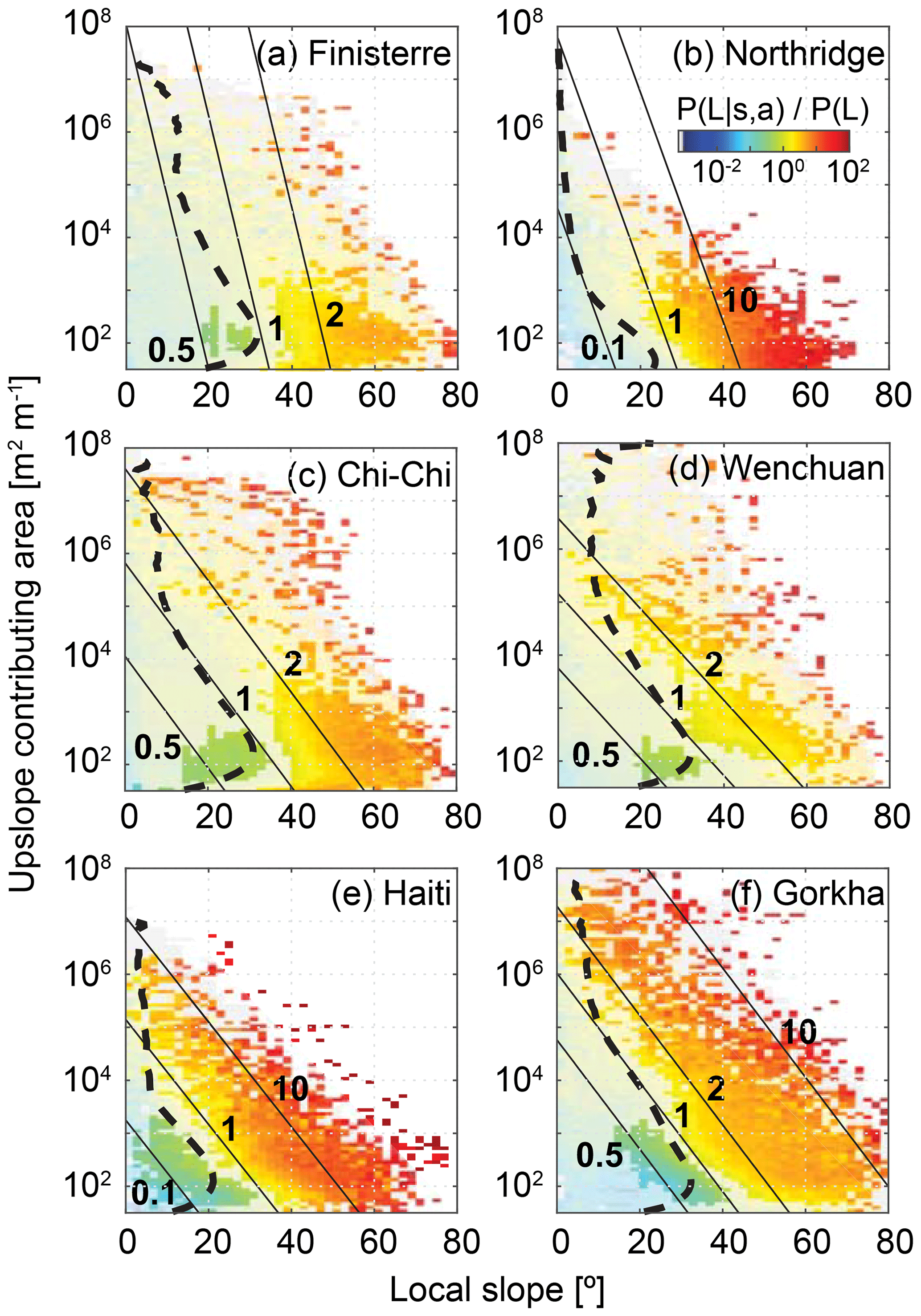
Figure 4Two-dimensional plots of landslide hazard defined as conditional landslide probability normalised by study area average landslide probability P(L), where s is local slope and a is upslope contributing area per unit cell width. Dashed lines show the mean slope per upslope contributing area bin, using 100 logarithmically spaced bins. Solid lines are landslide probability contours derived from logistic regression in the same units as the conditional landslide probability surface. Grey cells indicate slope–area pairs with data but with no cells touching a landslide. Note that upslope contributing area is shown on a logarithmic axis, so that maintaining a constant landslide probability for a given increase in slope requires a larger reduction in upslope contributing area at low slopes than at high slopes. Fainter colours indicate landslide hazard estimates that do not differ significantly from the study area average at 90 % confidence.
The model has two parameters (θm and θs), both of which are effective rather than measurable. We first optimise the model for each inventory to establish its performance under the best possible scenario, finding the values of θm and θs that provide the best fit to the inventory data. We then test the model using the average of the optimised parameters from the six inventories in order to represent a more realistic application wherein these parameters must be estimated from previous earthquakes. Thus, the values of θm and θs should not be interpreted as mechanistic thresholds but rather as the result of an optimisation that also depends on the DEM resolution.
6.1 Local slope
For all inventories, landslide hazard increases as an approximately exponential function of local slope (Fig. 3a). This behaviour is consistent up to slopes of 70∘, beyond which small sample sizes limit our confidence. Conditional probability exceeds the study area average landslide probability for slopes >30–35∘ in four of the inventories and for slopes >20–25∘ for the remaining two (Northridge and Haiti). This suggests that slopes <30∘ are generally safer than average, while those >45∘ have a landslide hazard >200 % of the average, and those >50∘ are generally >300 % of the average. The conditional probability curves for Finisterre, Chi-Chi and Gorkha largely collapse on each other when normalised by study area average probability (Fig. 3a). However, landslide hazard is less sensitive to slope for Wenchuan and more sensitive for Northridge and Haiti. This variability between inventories may be a result of weaker rock strength in the Northridge and Haiti study areas. When local slope is normalised by study area average slope (Fig. 3b), the curves collapse onto those from the other study areas. Comparing the combined PDF of study area slopes (Fig. 3a) with the hazard curves indicates that most landslide hazard is concentrated in a small subset of each study area (that is, on slopes >35∘). This implies that (1) many of the modest (<15∘) slopes on which people in these areas generally choose to live are exposed to relatively low hazard (less than half the study area average for all but Wenchuan), and (2) any decision to spend time or build infrastructure on steeper slopes should take into account the considerable associated increase in exposure to coseismic landslide hazard.
6.2 Upslope contributing area
For all inventories, the landslide hazard increases from less than the study area average at the lowest upslope contributing areas – that is, at the ridge tops – to a peak or plateau at intermediate upslope contributing areas (Fig. 3c). Locations with the lowest upslope contributing area also have the lowest hazard for four of the six inventories, with Northridge and Finisterre as exceptions. For Northridge, the zone of lower-than-average hazard extends only to upslope contributing areas of ∼40 m2 m−1; for Finisterre it extends to ∼100 m2 m−1, for Chi-Chi and Haiti to ∼150 m2 m−1, and for Wenchuan and Nepal to ∼200 m2 m−1. The location of peak landslide hazard broadly coincides with the inflection in average slope for a given upslope contributing area (Fig. 4). This inflection is commonly used as an indicator of the transition from hillslopes to rivers (Montgomery and Foufoula-Georgiou, 1993; Stock and Dietrich, 2003; Hancock and Evans, 2006), suggesting that maximum (or near-maximum) landslide hazard occurs at the transition from hillslopes to channels (Fig. 3c). We use this inflection to identify a reference upslope contributing area associated with channel initiation for each landscape. Normalising upslope contributing area by this reference area shifts the conditional probability curves laterally, aligning the Northridge curve with those from the other sites (Fig. 3d). This normalised analysis shows that landslide hazard is highest within low-order channels, where upslope contributing areas are less than 10 times the upslope contributing area associated with channel initiation in the study sites (Fig. 3d). Further downstream, landslide hazard generally decreases with increasing upslope contributing area, although limited sample sizes mean that we cannot confidently interpret the curves beyond ∼1000 m2 m−1.
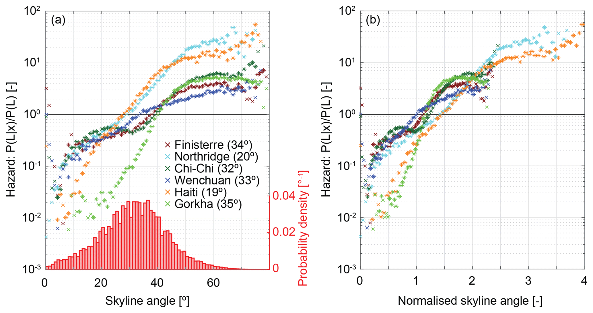
Figure 5Landslide hazard defined as conditional landslide probability normalised by study area average landslide probability for (a) skyline angle and (b) skyline angle normalised by the study area average. Asterisks indicate values for which conditional probability differs from the study area average probability at 90 % confidence. Red bars in (a) show histograms of skyline angle over the six inventories. Numbers in brackets show study area average skyline angles.
6.3 Local slope and upslope contributing area combined
When slope and upslope contributing area are examined in combination, the highest landslide hazard is consistently found at either the highest upslope contributing area for a given slope or the highest slope for a given upslope contributing area (Fig. 4). In this case normalisation adds little to our understanding of the relationship between landslide hazard and the two metrics under consideration, with normalised results shown in Fig. S9 for reference.
Two-dimensional conditional probability analysis is sensitive to the sample size within each bin, limiting our confidence in the results for large parts of the slope–upslope-contributing-area space. The logistic regression contours do not suffer the same limitation, however, and provide important additional information on the form of the relationship between landslide hazard, slope and upslope contributing area. Taken together, the logistic regression contours and conditional probability surfaces show that the lowest hazard is consistently found at locations with both low slope and low upslope contributing area. Importantly, landslide hazard increases more steeply with increasing slope than with increasing upslope contributing area, indicating the dominance of local slope in setting landslide hazard. There is some variability in the orientation of the hazard contours between inventories, with Finisterre and Northridge showing the strongest slope dependence and Wenchuan showing the strongest upslope contributing area dependence (Fig. 4).
The shape of the two-dimensional probability surface determines the best course of action in terms of choosing alternative locations for a particular asset or activity, but such action is also constrained by what is possible. The average slopes for each upslope contributing area (shown by the dashed lines in Fig. 4) indicate that for Northridge, Finisterre, Chi-Chi and Haiti, there are rarely situations in which a reduction in upslope contributing area will not involve (on average) an increase in slope that will actually increase landslide hazard. However, for locations in Wenchuan and Gorkha with upslope contributing areas of 300 to 10 000 m2 m−1, the hazard reduction due to reducing upslope contributing area is not offset by the associated increase in slope. This suggests that, for the former inventories, it is always beneficial to decrease slope, even at the expense of upslope contributing area, while for the latter inventories the benefit is more dependent on initial location. In general, the average slope contour appears to separate higher- and lower-than-average landslide hazard in slope–upslope-contributing-area space, suggesting that higher-than-average landslide hazard is consistently found on higher-than-average slopes for a given upslope contributing area.
6.4 Skyline angle
Landslide hazard increases as an approximately exponential function of maximum skyline angle (Fig. 5a), similarly to the relationship with local slope (Fig. 3a). We are confident in this behaviour for skyline angles in the range 5 to 70∘, outside of which small sample sizes limit our confidence. Landslide hazard exceeds the study area average at skyline angles >27–28∘ for Northridge and Haiti, 34∘ for Wenchuan, and 38–40∘ for Finisterre, Chi-Chi and Gorkha. Locations with skyline angles of <20∘ have less than half the study area average landslide hazard for all inventories, while those with skyline angles of >50∘ have more than double the study area average (Fig. 5a). The lowest landslide hazard values, at skyline angles of less than 10∘, are lower than those for local slope or upslope contributing area. As with local slope, the curves for several of the inventories (Finisterre, Chi-Chi and Wenchuan) collapse to a similar relationship when normalised by study area average hazard, suggesting similar behaviour across a range of different landscapes. However, Northridge and Haiti show stronger sensitivity to skyline angle, and Gorkha shows considerably reduced landslide hazard at low skyline angles, relative to the other inventories. Some of this variability between inventories is likely related to differences in rock strength, because normalising skyline angle by the study area average considerably reduces the separation between individual curves, particularly those for Gorkha, Northridge and Haiti (Fig. 5b).
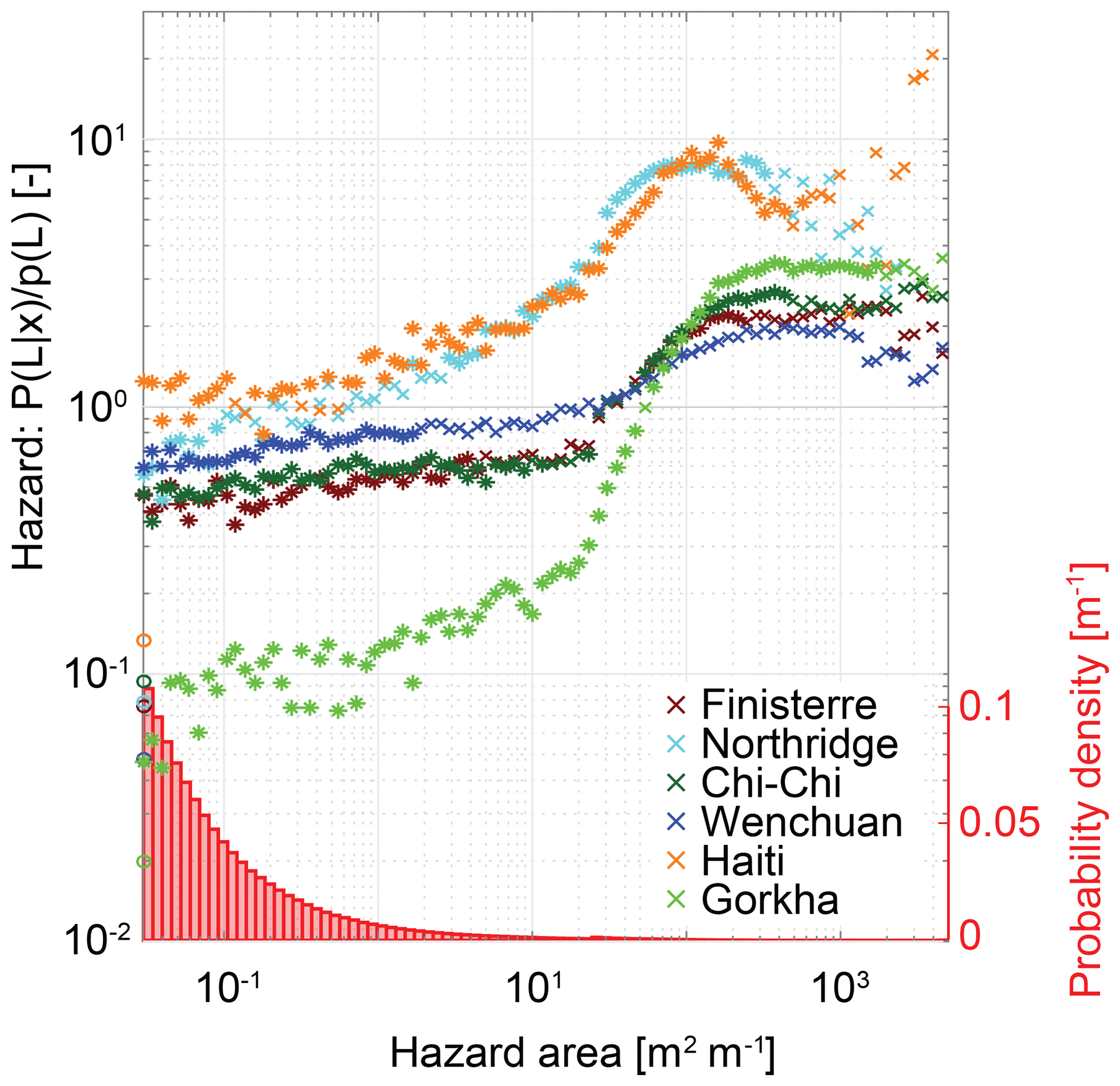
Figure 6Landslide hazard defined as the conditional landslide probability P(L|x) normalised by study area average landslide probability P(L) for the hazard area. Hazard area is calculated with global average parameters θm and θs – that is, the areas with slope greater than 40∘ that have a flow path to the cell of interest and do not travel across a cell with a slope less than 10∘. Coloured circles on the y axis indicate landslide hazard for cells with a hazard area of 0 m2 m−1. Asterisks indicate values for which probability differs from the study area average at 90 % confidence. Red bars show histograms of hazard area over the six inventories.
6.5 Hazard area
The ability of hazard area Ah to distinguish landslide cells from non-landslide cells is sensitive to two tuneable parameters (θm and θs in Eqs. 6 and 7) that have a unique optimum for each inventory (Fig. S1). The optimum parameter values vary between inventories, with optimum initiation slopes θm ranging from 36 to 40∘ and stopping slopes θs from 6 to 31∘ (Table S1). Since these optimum parameters vary between inventories and can only be identified after an earthquake, they are problematic in terms of incorporation into a rule. Instead, we use the global averages of the optimised parameter values from the six inventories, θm=40∘ and θs=10∘, rounded to one significant figure to simplify the rule (and because it involves changing only θm from 39 to 40∘). The stopping angle of 10∘ is steeper than many, though not all, of the observed slopes on which debris flows stop. For example, Stock and Dietrich (2003) reported that debris flows generally exhibit stopping angles of 2–6∘ but may halt at much larger angles (13–22∘) on open slopes. The steeper angles reported here may reflect differences in the method and resolution of slope calculation but may result from the coseismic trigger, which does not necessitate high levels of saturation in the initial failure. Landslide hazard is very low for cells with Ah=0 (i.e. where no cells steeper than the initiation angle run-out over flow paths steeper than the stopping angle), ranging from 2 % to 15 % of the study area average (Fig. 6). Hazard increases with increasing Ah for all inventories but only slowly for Ah<20 m2 m−1; the trend then steepens to a peak (Northridge, Haiti, Nepal) or plateau (Finisterre, Chi-Chi, Wenchuan) at Ah values of ∼100 to 1000 m2 m−1 with conditional probabilities that are 200 %–800 % of the study area average (Fig. 6). For Finisterre and Wenchuan, a combination of limited observations and a weaker dependence of landslide probability on hazard area results in large parts of the curve (at Ah>1 m2 m−1) where conditional probabilities cannot be distinguished from the study area average. For all sites, confidence becomes weak for hazard areas greater than 1000 m2 m−1.
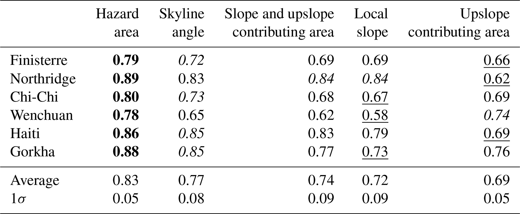
Table 1Area under the ROC curve for the five hazard metrics over the six coseismic landslide inventories. The best-performing metric for each inventory is in bold, the second best is in italics and the worst-performing metric is underlined.
6.6 ROC analysis
To supplement conditional probability analysis, we examine the performance of slope, upslope contributing area, skyline angle and hazard area as continuous hazard indices (with high index values reflecting high hazard and vice versa) using ROC curves (Fig. 7). Successful hazard indices will capture landslide cells within high index zones (true positives) without capturing non-landslide cells in the same zones (false positives). Hazard area performs best for all six inventories with an AUC always above 0.78 and an average AUC of 0.83 (Table 1). Skyline angle performs joint best for Haiti and second best for a further three of the six inventories, with AUC always above 0.65 and an average AUC of 0.77. The exceptions, where slope, upslope contributing area or their combination performs second best, are Northridge and Wenchuan. For Northridge, slope alone and slope plus upslope contributing area both outperform skyline angle by a single percentage point, while upslope contributing area alone performs considerably worse (Fig. 7b). For Wenchuan, upslope contributing area considerably outperforms the other indices, while slope performs particularly poorly, perhaps reflecting longer-run-out landslides that extend to lower slopes and larger areas (Fig. 7d). Although slope, upslope contributing area and their combination all perform better than skyline angle in one of the inventories, none of these metrics does so consistently across multiple inventories. This is reflected in their averaged AUC values over all inventories of 0.69, 0.72 and 0.74 for upslope contributing area, slope and their combination respectively.
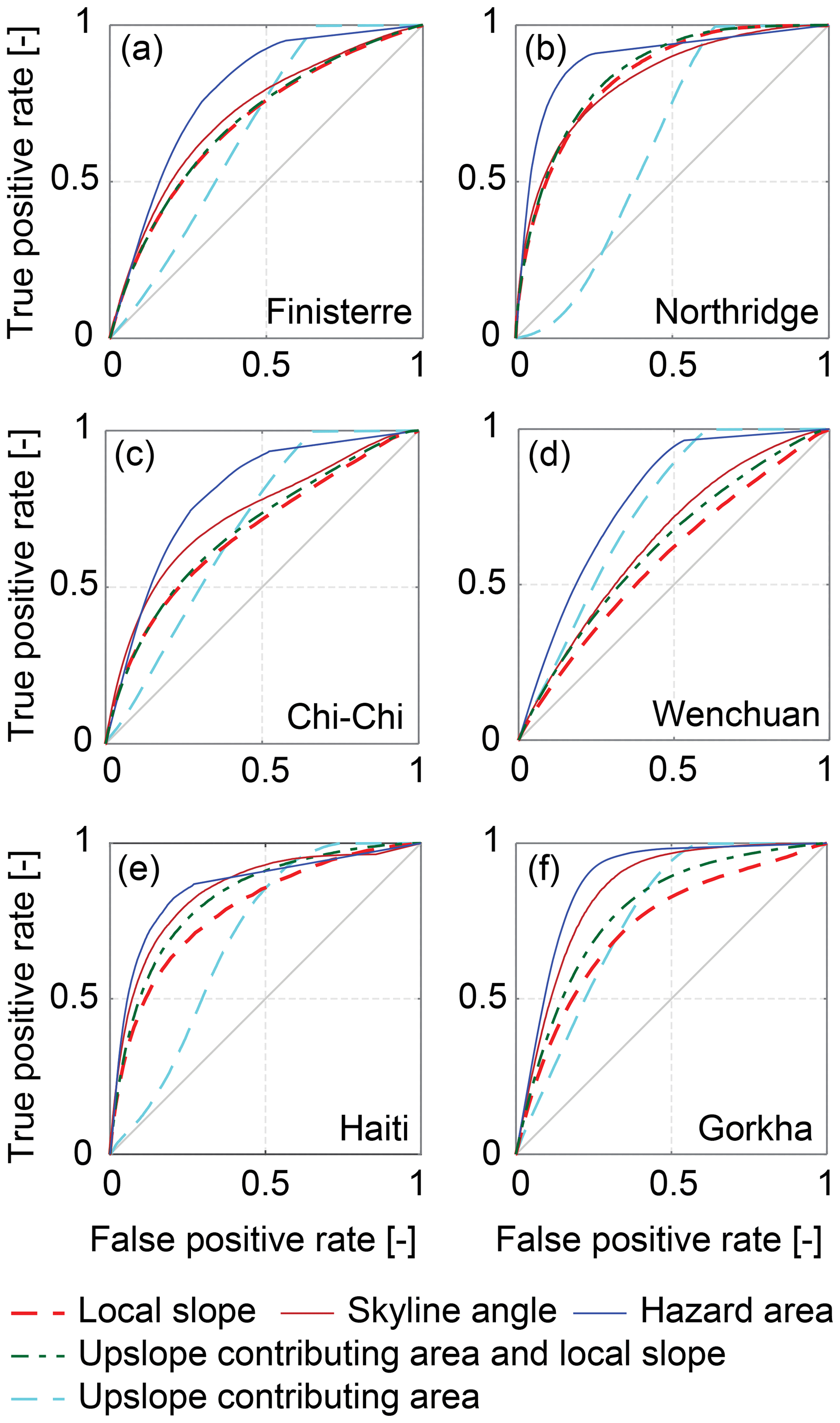
Figure 7Receiver operating characteristic (ROC) curves for the six inventories: (a) Finisterre, (b) Northridge, (c) Chi-Chi, (d) Wenchuan, (e) Haiti and (f) Gorkha. False positive rate is given by the number of false positives divided by the sum of false positives and true negatives. True positive rate is given by the number of true positives divided by the sum of true positives and false negatives. The 1:1 line represents the naïve random case. Curves plotting closer to the top-left corner of each panel represent better model performance.
We structure the discussion around three simple rules that are drawn from the results above. In each case we explain the evidence on which the message is based, why it works, our degree of confidence and implications for applying the rule. Finally, we examine the spatial implications of these rules using an example landscape.
7.1 Rule 1: Avoid steep (>10∘) channels with many steep (>40∘) areas that are upslope
The hazard area is the best or joint-best predictor of landslide hazard for all six inventories. The hazard area defined by the average initiation angle (40∘) and stopping angle (10∘) across all six inventories performs nearly as well as the optimised area for each inventory, enabling us to define a general rule independent of any specific inventory. This is fortunate, as site-specific optimisation requires a pre-existing landslide inventory for any individual area and so may not be generally feasible. In all six inventories, locations with Ah>60 m2 m−1 have landslide hazard that is greater than the study area average. While landslide hazard generally increases with increasing hazard area, the relationship is complex (Fig. 6). Landslide hazard can be most effectively decreased by decreasing Ah in the range 20–100 m2 m−1. Outside this range Ah is less related to hazard. An exception to this pattern is seen in areas with a hazard area of zero, which generally have landslide hazard 5–10 times lower than that for even very small values of Ah (ca. 0.1 m2 m−1). On this basis, the qualitative statement to avoid areas with “many” steep slopes could also be phrased as “any” steep slopes.
7.2 Rule 2: Minimise your maximum angle to the skyline
The maximum skyline angle is the second-best predictor of landslide hazard in four of the six cases. Locations with skyline angles less than 30∘ generally have a landslide hazard below the study area average. Importantly, landslide hazard increases non-linearly with skyline angle, so that a slight reduction to a high skyline angle results in a much larger reduction in hazard than a similar reduction to a lower skyline angle.
The distinction between local slope and skyline angle reflects the importance of run-out as well as initiation in defining landslide hazard. Landslide hazard is an inherently non-local problem, defined by both conditions at the point of interest and those upslope of that point. The skyline angle is a simple way to represent this. It has the additional advantage of being easy to measure, needing only a protractor or clinometer for precise measurement in the field and being easily approximated by eye. Local slope (rule 3), in contrast, is scale dependent, while hazard area Ah (rule 1) is considerably more difficult to estimate in the field.
Landslides do not always obey flow path routing rules, and it is possible for landslides to travel up reverse slopes or along contours. This is particularly true for large deep-seated landslides or rockfalls. The hazard area metric cannot account for such behaviour and thus is more likely to reflect hazard from smaller shallow landslides, while skyline angle, which does allow for run-out over reverse slopes, may be a better predictor of larger deep-seated landslides. The two indices have some overlap but could be used in combination to find safer locations in the landscape.
7.3 Rule 3: Minimise the angle of the slope under your feet, especially on steep hillsides, but not at the expense of increasing skyline angle or hazard area
Local slope generally performs less well than skyline angle or hazard area but is still a consistently skilful predictor of coseismic landslide hazard and could be a useful additional discriminant for situations where both skyline angle and hazard area are comparable between two locations. In this situation, our results suggest choosing the location with the lower local slope. This is particularly true at steeper slopes, since landslide hazard increases exponentially with slope, approximately doubling for every 10∘ increase in slope.
Given the observation from a number of landslide inventories that coseismic landslides initiate near ridge crests (Densmore and Hovius, 2000; Meunier et al., 2008; Rault et al., 2018), it is perhaps surprising that landslide hazard generally increases with increasing upslope contributing area (i.e. when moving downslope from ridge crests). In fact, while coseismic landslides may initiate preferentially near the ridges, they run out downslope; thus, areas near ridges are less likely to be touched by any part of a landslide, even though they are more likely than other parts of the landscape to contain the top of a landslide scar. Landslide hazard is consistently low at small values of upslope contributing area, corresponding to ridges; for some inventories, it is also low at very large values of upslope contributing area, corresponding to valley floors in the downstream reaches of the river network. This may be partly a function of the covariance between local slope and upslope contributing area, because locations with large upslope contributing areas generally have lower slopes (see dashed lines in Fig. 4). The addition of upslope contributing area as a predictor in logistic regression improves landslide hazard prediction relative to slope alone (Table 1), but the orientation of the logistic regression contours (Fig. 4) indicates that its influence is weak. Moving to a location with lower slope angle almost always reduces landslide hazard independently of the upslope contributing area of the new location, although the specific reduction of landslide probability depends on the shape of the two-dimensional probability surface (Fig. 4). These results suggest that decisions on how to reduce landslide hazard most effectively need to be made on a case by case basis, and they are best made using hazard area, skyline angle and local slope in conjunction with each other. Steep areas that are upslope of a given location result in an elevated hazard but gentle areas do not, explaining the improved performance of hazard area relative to upslope contributing area (Fig. 6 and Table 1). Ridges, with very low upslope contributing area, are generally low-hazard locations if they have gentle local slope but can still be hazardous if they are steep (Fig. 4). To minimise landslide hazard, it is thus preferable to seek broad ridges over sharp ridges where such a choice is possible.
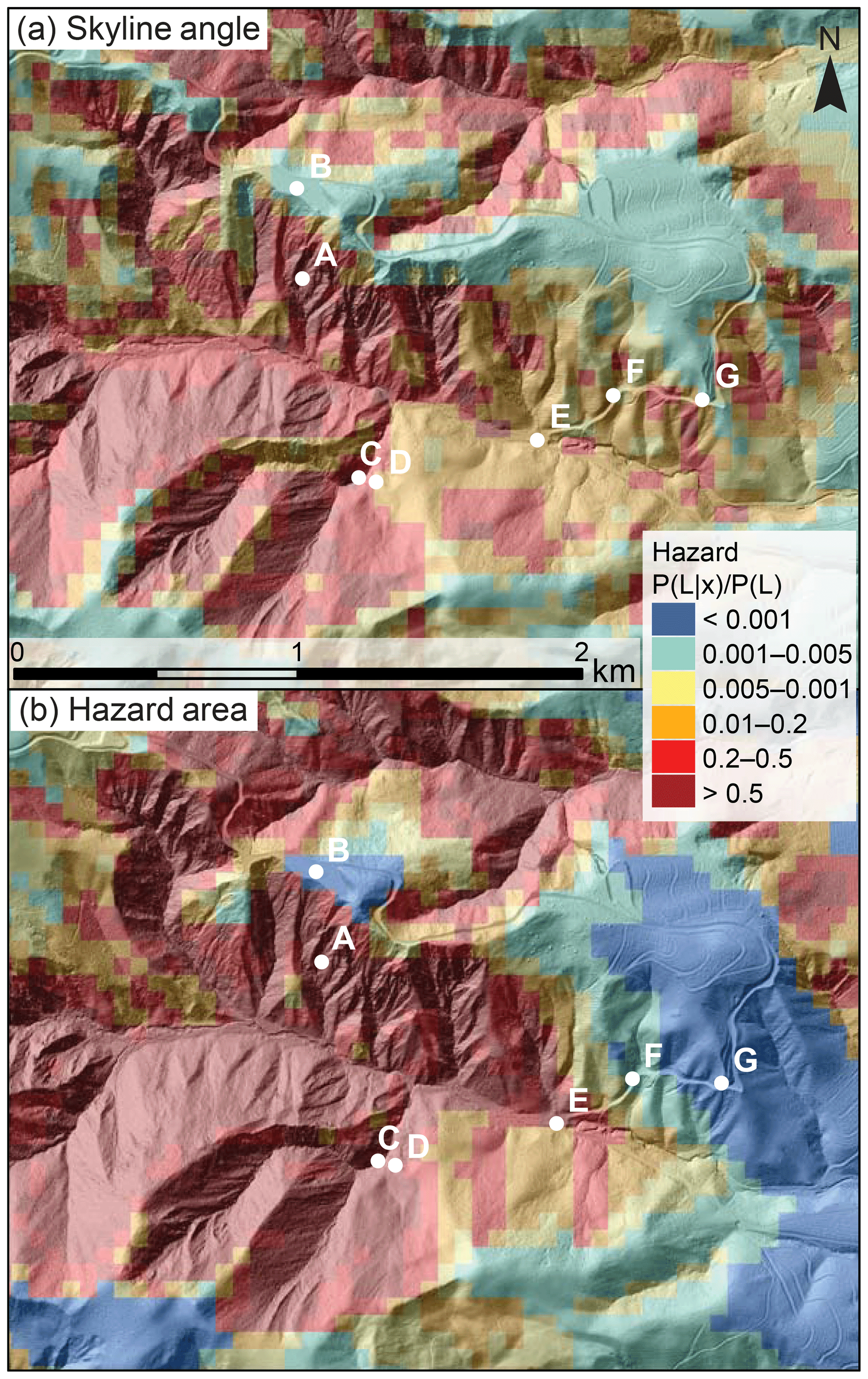
Figure 8Example landslide hazard estimates derived from (a) skyline angle and (b) hazard area for a small section of the Northridge study area. Colours reflect landslide hazard estimated from the two methods, expressed as a fraction of the study area average hazard. Points labelled A–G in white are example locations discussed in Sect. 7.4. Hazard estimates are overlain on a shaded-relief image derived from a 0.5 m resolution lidar DEM for context (source: NCALM, 2015, http://opentopo.sdsc.edu/datasetMetadata?otCollectionID=OT.072016.32611.1, last access: 29 March 2019).
7.4 Movement rules in a landscape with variable hazard
Our analysis is focused on cell-by-cell hazard assessment and is thus most appropriate for decision-making before the next large earthquake. However, it is also possible to use our results to inform movement or relocation during or immediately after an earthquake, when it is likely that movement will be limited to small distances. Our analysis shows that, even during a large earthquake in mountainous terrain, landslide hazard is not ubiquitously high. A significant fraction of the landscape has low landslide hazard (<5 % of the study area average) – as much as 30 % in Northridge and 33 % in Nepal. Landslide hazard is extremely granular in spatial terms, so that small changes in location can make a big difference to exposure. This means that it is often possible to find nearby locations with lower landslide hazard, irrespective of the starting point. The vast majority of locations (75 % in Nepal, 95 % in Northridge) are within 1 km of areas of low landslide hazard (<5 % of the study area average). Even smaller movements of 100 m or less, as might be possible during or immediately after a large earthquake, can result in very large reductions in hazard.
Detailed analysis in the Northridge (Fig. 8) and Nepal inventories shows that landslide hazard can often be effectively reduced by moving from a slope to a ridge (e.g. from A to B in Fig. 8, a 190 % reduction in landslide hazard), out of a gully (e.g. from C to D, a 100 % reduction) or downstream of a flatter area (e.g. from C to E, a 100 % reduction). However, there is no single answer to the question of where to move to reduce coseismic landslide hazard, since this differs depending on the setting, the distance that can be travelled due to time or location constraints and on the chosen rule (e.g. skyline angle vs. hazard area). Given a 1 km radius of potential movement, minimising the skyline angle involves moving upslope for ∼75 % of locations in Nepal but only ∼66 % in Northridge. In some cases, knowing how far one can travel can be critical: if one may only travel a short distance, moving upslope may be preferable (e.g. from C to D in Fig. 8, a 100 % reduction), while if one could travel farther, moving downslope may offer greater hazard reduction (e.g. from C to F or G, a 120 % or 190 % reduction respectively).
Landslide hazard estimates for high-hazard locations are broadly comparable between skyline angle and hazard area metrics (e.g. Fig. 8). However, different metrics emphasise different parts of the landscape. Ridges consistently minimise skyline angle but may still have intermediate values of hazard area if the ridge is sharp so that the local slope of the ridge itself is steep. Broad valley floors consistently minimise hazard area but may still have intermediate values of skyline angle if the neighbouring slopes have sufficient relief. There are trade-offs between these metrics, and further work is needed into how they might be combined to further reduce hazard.
7.5 Caveats
These rules should be combined with existing guidance, such as local knowledge and formal hazard and risk information when that is available. The rules provide an evidence base that could be used, for example, in infrastructure and land-use planning for identifying evacuation routes and designing contingency plans from individual to community level, where more detailed or formal technical advice is not available. It is also important to note some caveats.
This analysis is purely focused on coseismic landslide hazard, and thus it does not take into account the distribution of vulnerability: that is, the locations of people and infrastructure in these landscapes or how they might be differentially impacted by landslides. While one area may be more hazardous than another, the distribution of people and infrastructure may be such that risk is not actually increased. Further, our analysis is probabilistic, defining hazard as the probability of intersecting a landslide; thus, our rules identify locations where the landslide probability is lower, not where probability is zero. This means that it is possible for an alternate location chosen based on its lower landslide probability to be impacted by a landslide, while the original higher-probability location is not. The choice of inventory will influence the specific results and, although we adjust for bulk shaking intensity by normalising conditional probability by bulk probability, differences between inventories are likely to remain (e.g. in spatial patterns of shaking intensity and their relation to topography). Rock type is a critical influence on landslide occurrence (Chen et al., 2012; Harp et al., 2016; Roback et al., 2018), but we have excluded it from our analysis because it is extremely difficult for an untrained observer to identify and to translate it into meaningful estimates of material strength and thus landslide probability. We also expect that the length scales over which lithology varies will often be long (on the order of kilometres) relative to the other factors examined here.
Because the analysis is focused on coseismic landslide hazard, it does not account for other sources of hazard, either associated with an earthquake (e.g. amplification of seismic accelerations on ridges) or with other processes or events such as flooding or rainfall-induced landsliding. In some cases, following our rules in isolation might increase exposure to other hazards. For example, moving to ridge tops to minimise skyline angle might increase exposure to intense shaking due to seismic amplification in subsequent earthquakes; moving to valley floors that are occupied by large rivers, where hazard area is minimal, might increase exposure to fluvial flooding. We have also not considered the effects of landslide size or failure type, choosing instead to treat all landslides as representing an equivalent hazard. If landslide size or type shows a strong spatial dependence, then parts of the landscape may be preferentially impacted in ways that are not reflected by our rules. It is not yet clear how transferrable our conditional probability results are to rainfall-triggered landslides. For instance, stopping angles are likely to be lower for rainfall-triggered landslides if the failing mass is more highly saturated (e.g. Stock and Dietrich, 2003), meaning that the hazard area in rule 1 underestimates potential landslide impacts. Similarly, in the case of rainfall-triggered landslides, initiation is likely to depend not only on slope angle but also on a topographic control on saturation (e.g. Montgomery and Dietrich, 1994). Extending the analysis to other triggering mechanisms is thus a future research need.
We have evaluated these rules using gridded topographic data and landslide inventories. Topographic derivatives, particularly slope and upslope contributing area, are known to be sensitive to the resolution of the DEM from which they are derived. We use the Northridge study site to begin to explore this issue by repeating our analysis with DEMs at both the original 10 m resolution and at resampled resolutions of 20, 30, 60 and 90 m. We find that the performance of slope, skyline angle and upslope contributing area all improve slightly at finer resolutions (Table S3). Hazard area performance degrades at both finer and coarser resolutions than 30 m, which is likely the result of parameter optimisation being performed at 30 m resolution. We still find, however, that the hazard area metric remains the most skillful predictor of landslide hazard across all DEM resolutions.
The accuracy of landslide inventories depends on the quality of the imagery from which they are mapped and on subjective judgements by the mappers (Williams et al., 2018). For example, there are uncertainties associated with landslide distinction and amalgamation (Marc and Hovius, 2015; Tanyas et al., 2017) and the definition of the downslope boundary of each landslide. Amalgamation is particularly problematic for landslide volume estimates but less so in our analysis, which requires identification of landslide-affected areas rather than distinguishing individual landslides. However, recent studies have identified substantial areal mismatches (up to 67 %) between inventories of the same event mapped by different authors (Fan et al., 2019). To investigate the impact of mapping error on our results, we test two independent inventories for the Wenchuan earthquake, from Li et al. (2014) and Xu et al. (2014b), with an estimated areal mismatch for our study area of 21 %. We find that the change of inventory has no impact on the rank order of performance of the metrics (Table S3) and a minor impact on both the AUC values and the hazard curves (Figs. S10 and S11). Thus, we suggest that our findings are relatively robust to mapping uncertainties in the landslide inventories that we have used.
We have defined a set of simple rules that can be used to anticipate, and thus potentially reduce, exposure to earthquake-triggered landslides. We test a set of candidate predictors for their ability to reproduce mapped landslide distributions from six recent earthquakes. Landslide hazard, defined as the conditional probability of intersecting a landslide in one of the six earthquakes, increases exponentially with local slope. Landslide hazard on hillslopes also increases with upslope contributing area, suggesting that, while ridges may be areas of preferential coseismic landslide initiation, they are not the locations of highest coseismic landslide hazard due to downslope movement of landslide material during run-out. When accounting for both slope and upslope contributing area, landslide hazard is highest for the largest upslope contributing area at a given slope or the highest slope at a given upslope contributing area. Landslide hazard can be reduced by decreasing local slope, even at the cost of increased upslope contributing area and especially at high slopes. Landslide hazard also increases exponentially with the skyline angle, and this simple, easily measured metric performs better than slope or upslope contributing area for four of the six inventories. Hazard area, which accounts for both landslide initiation and run-out, offers the best predictive skill for all six inventories but is more difficult to estimate in the field and requires estimation of two empirical parameters. Fortunately, hazard area calculated with parameters that are averaged across all six study sites (initiation angle of 40∘ and stopping angle of 10∘) performs almost as well as hazard area calculated with optimised site-specific parameters, suggesting that the average parameters can be applied to other inventories. These findings can be distilled into three simple rules:
-
avoid steep (>10∘) channels with many steep (>40∘) areas that are upslope;
-
minimise your maximum angle to the skyline;
-
minimise the angle of the slope under your feet, especially on steep hillsides, but not at the expense of increasing skyline angle or hazard area.
Landslide inventories for Northridge (Harp and Jibson, 1996), Haiti (Harp et al., 2017), Wenchuan (Li et al., 2014; Xu et al., 2014b) and Gorkha (Roback et al., 2018) were retrieved from the online USGS ScienceBase-Catalog: (https://www.sciencebase.gov/catalog/item/586d824ce4b0f5ce109fc9a6, last access: 29 March 2019). Landslide inventories for Finisterre (Meunier et al., 2007) and Chi-Chi (Dadson et al., 2004) were obtained from the authors.
The SRTM-30 m DEM data (NASA JPL, 2013) are available from the online Global Data Explorer (https://gdex.cr.usgs.gov/gdex/, last access: 29 March 2019). The lidar DEM data (NCALM, 2015) are available from OpenTopography (http://opentopo.sdsc.edu/datasetMetadata?otCollectionID=OT.072016.32611.1, last access: 29 March 2019).
The supplement related to this article is available online at: https://doi.org/10.5194/nhess-19-837-2019-supplement.
DM and ALD conceived the study. DB and DM conceived the modified SHALRUN model. DM collated and analysed all data. DM and ALD wrote the paper with assistance and input from DB, NR, JW, GL and KO.
The authors declare that they have no conflict of interest.
This work was financially supported by grants from the NERC/ESRC Increasing Resilience to Natural Hazards programme (NE/J01995X/1) and the NERC/ESRC/NNSFC Increasing Resilience to Natural Hazards in China programme (NE/N012216/1). We thank (1) colleagues at the National Society for Earthquake Technology-Nepal (NSET) who have helped to shape our thinking on landslide hazard and the challenge of risk communication; (2) those responsible for collecting the landslide inventories used in this study, particularly Niels Hovius and contributors to the ScienceBase-Catalog; and (3) William Dietrich and Niels Hovius for helpful comments on an earlier draft. Gianvito Scaringi, Odin Marc and an anonymous reviewer provided constructive and illuminating comments and suggestions that considerably refined our thinking. Lidar data acquisition and processing were completed by the National Center for Airborne Laser Mapping (NCALM). NCALM funding was provided by NSF's Division of Earth Sciences, Instrumentation and Facilities Program (EAR-1043051). MATLAB code for the computation of skyline angles is available at https://github.com/DavidMilledge (last access: 29 March 2019).
This paper was edited by Thom Bogaard and reviewed by Odin Marc and one anonymous referee.
Alexander, D.: Vulnerability to landslides, in: Landslide Hazard and Risk, Wiley, Chichester, 175–198, 2005.
Atwater, B. F., Cisternas, M. V., Bourgeois, J., Dudley, W. C., Hendley, J. W., and Stauffer, P. H.: Surviving a tsunami – lessons from Chile, Hawaii, and Japan, No. 1187, Geological Survey (USGS), 1999.
Avouac, J. P., Meng, L., Wei, S., Wang, T., and Ampuero, J. P.: Lower edge of locked Main Himalayan Thrust unzipped by the 2015 Gorkha earthquake, Nat. Geosci., 8, 708–711, 2015.
Bellugi, D., Dietrich, W. E., Stock, J., McKean, J., Kazian, B., and Hargrove, P.: Spatially explicit shallow landslide susceptibility mapping over large areas, Proceedings of the 5th International Conference on Debris-Flow Hazards Mitigation: Mechanics, prediction and assessment, Italian Journal of Engineering Geology and Environment, 759–768, doi:10.4408/IJEGE.2011-03.B-045, 2011.
Benda, L. E. and Cundy, T. W.: Predicting deposition of debris flows in mountain channels, Can. Geotech. J., 27, 409–417, 1990.
Berti, M., Martina, M. L. V., Franceschini, S., Pignone, S., Simoni, A., and Pizziolo, M.: Probabilistic rainfall thresholds for landslide occurrence using a Bayesian approach, J. Geophys. Res.-Earth, 117, F04006, https://doi.org/10.1029/2012JF002367, 2012.
Blöthe, J. H., Korup, O., and Schwanghart, W.: Large landslides lie low: Excess topography in the Himalaya-Karakoram ranges, Geology, 43, 523–526, 2015.
Briggs, J.: The use of indigenous knowledge in development: problems and challenges, Prog. Dev. Stud., 5, 99–114, 2005.
Chen, X. L., Ran, H. L., and Yang, W. T.: Evaluation of factors controlling large earthquake-induced landslides by the Wenchuan earthquake, Nat. Hazards Earth Syst. Sci., 12, 3645–3657, https://doi.org/10.5194/nhess-12-3645-2012, 2012.
Claessens, L., Heuvelink, G. B. M., Schoorl, J. M., and Veldkamp, A.: DEM resolution effects on shallow landslide hazard and soil redistribution modelling, Earth Surface Processes and Landforms, 30, 461–477, 2005.
Corominas, J.: The angle of reach as a mobility index for small and large landslides, Can. Geotech. J., 33, 260–271, 1996.
Dadson, S. J., Hovius, N., Chen, H., Dade, W. B., Hsieh, M. L., Willett, S. D., Hu, J. C., Horng, M. J., Chen, M. C., Stark, C. P., and Lague, D.: Links between erosion, runoff variability and seismicity in the Taiwan orogen, Nature, 426, 648–651, 2003.
Dadson, S. J., Hovius, N., Chen, H., Dade, W. B., Lin, J. C., Hsu, M. L., Lin, C. W., Horng, M. J., Chen, T. C., Milliman, J., and Stark, C. P.: Earthquake-triggered increase in sediment delivery from an active mountain belt, Geology, 328, 733–736, 2004
Dai, F. C., Xu, C., Yao, X., Xu, L., Tu, X. B., and Gong, Q. M.: Spatial distribution of landslides triggered by the 2008 Ms 8.0 Wenchuan earthquake, China, J. Asian Earth Sci., 40, 883–895, 2011.
Datta, A., Sigdel, S., Oven, K., Rosser, N., Densmore, A., Rijal, S.: The role of scientific evidence during the 2015 Nepal earthquake relief efforts, Overseas Development Institute: London, UK, 2018.
Densmore, A. L., Ellis, M. A., and Anderson, R. S.: Landsliding and the evolution of normal-fault-bounded mountains, J. Geophys. Res.-Earth, 103, 15203–15219, 1998.
Densmore, A. L. and Hovius, N.: Topographic fingerprints of bedrock landslides, Geology, 28, 371–374, 2000.
Dietrich, W. E. and Sitar, N.: Geoscience and geotechnical engineering aspects of debris-flow hazard assessment, in: Debris-flow hazards mitigation: Mechanics, prediction, and assessment, ASCE, 656–676, 1997.
Dransch, D., Rotzoll, H., and Poser, K.: The contribution of maps to the challenges of risk communication to the public, Int. J. Digit. Earth, 3, 292–311, 2010.
Elliott, J. R., Jolivet, R., González, P. J., Avouac, J. P., Hollingsworth, J., Searle, M. P., and Stevens, V. L.: Himalayan megathrust geometry and relation to topography revealed by the Gorkha earthquake, Nat. Geosci., 9, p. 174, 2016.
Fan, X., Scaringi, G., Domènech, G., Yang, F., Guo, X., Dai, L., He, C., Xu, Q., and Huang, R.: Two multi-temporal datasets that track the enhanced landsliding after the 2008 Wenchuan earthquake, Earth Syst. Sci. Data, 11, 35–55, 2019.
Fannin, R. J. and Wise, M. P.: An empirical-statistical model for debris flow travel distance, Can. Geotech. J., 38, 982–994, 2001.
Fell, R., Ho, K. K., Lacasse, S., and Leroi, E.: A framework for landslide risk assessment and management, Landslides, 3–25, 2005.
Froude, M. J. and Petley, D. N.: Global fatal landslide occurrence from 2004 to 2016, Nat. Hazards Earth Syst. Sci., 18, 2161–2181, https://doi.org/10.5194/nhess-18-2161-2018, 2018.
George, D. L. and Iverson, R. M.: A depth-averaged debris-flow model that includes the effects of evolving dilatancy: 2. Numerical predictions and experimental tests, P. Roy. Soc. A-Math. Phy., 470, 20130820, https://doi.org/10.1098/rspa.2013.0819, 2014.
Fell, R., Ho, K. K., Lacasse, S., and Leroi, E.: A framework for landslide risk assessment and management, in: Landslide Risk Management, edited by: Hungr, O., Fell, R., Couture, R., and Eberhardt, E., CRC Press, Boca Raton, Florida, USA, 3–25, 2005.
Frattini, P., Crosta, G., and Carrara, A.: Techniques for evaluating the performance of landslide susceptibility models, Eng. Geol., 111, 62–72, 2010.
Geller, R. J.: Earthquake prediction: a critical review, Geophys. J. Int., 131, 425–450, 1997.
Gigerenzer, G.: Why heuristics work, Perspect. Psychol. Sci., 3, 20–29, 2008.
Gorum, T., Fan, X., van Westen, C. J., Huang, R. Q., Xu, Q., Tang, C., and Wang, G.: Distribution pattern of earthquake-induced landslides triggered by the 12 May 2008 Wenchuan earthquake, Geomorphology, 133, 152–167, 2011.
Gorum, T., Korup, O., van Westen, C. J., van der Meijde, M., Xu, C., and van der Meer, F. D.: Why so few? Landslides triggered by the 2002 Denali earthquake, Alaska, Quat. Sci. Rev., 95, 80–94, 2014.
Guillard-Gonçalves, C., Zêzere, J. L., Pereira, S., and Garcia, R. A. C.: Assessment of physical vulnerability of buildings and analysis of landslide risk at the municipal scale: application to the Loures municipality, Portugal, Nat. Hazards Earth Syst. Sci., 16, 311–331, https://doi.org/10.5194/nhess-16-311-2016, 2016.
Hancock, G. R. and Evans, K. G.: Channel head location and characteristics using digital elevation models, Earth Surf. Proc. Land., 31, 809–824, 2006.
Harp, E. L., Wilson, R. C., and Wieczorek, G. F.: Landslides from the 4 February 1976, Guatemala earthquake, No. 551.3 HAR, US Government Printing Office, 1981.
Harp, E. L. and Jibson, R. W.: Landslides triggered by the 1994 Northridge, California, earthquake, B. Seismol. Soc. Am., 86, 319–332, 1996.
Harp, E. L., Jibson, R. W., and Schmitt, R. G.: Map of landslides triggered by the 12 January 2010, Haiti earthquake: U.S. Geological Survey Scientific Investigations Map 3353, https://doi.org/10.3133/sim3353, 15 pp., 2016.
Harp, E. L., Jibson, R. W., and Schmitt, R. G.: Map of landslides triggered by the 12 January 2010, Haiti earthquake, https://doi.org/10.5066/F7C827SR, in: An Open Repository of Earthquake-triggered Ground Failure Inventories, in Schmitt, R.G., Tanyas, H., Nowicki Jessee, M. A., Zhu, J., Biegel, K. M., Allstadt, K. E., Jibson, R. W., Thompson, E. M., van Westen, C. J., Sato, H. P., Wald, D. J., Godt, J. W., Gorum, T., Xu, C., Rathje, E. M., and Knudsen, K. L., U.S. Geological Survey data release collection, 2018, doi:10.5066/F7H70DB4, 2017.
Hauksson, E., Jones, L. M., and Hutton, K.: The 1994 Northridge earthquake sequence in California: Seismological and tectonic aspects, J. Geophys. Res.-Earth, 100, 12335–12355, 1995.
Hayes, G. P., Briggs, R. W., Sladen, A., Fielding, E. J., Prentice, C., Hudnut, K., Mann, P., Taylor, F. W., Crone, A. J., Gold, R., and Ito, T.: Complex rupture during the 12 January 2010 Haiti earthquake, Nat. Geosci., 3, 800–805, 2010.
Hayes, G. P., Briggs, R. W., Barnhart, W. D., Yeck, W. L., McNamara, D. E., Wald, D. J., Nealy, J. L., Benz, H. M., Gold, R. D., Jaiswal, K. S., and Marano, K.: Rapid characterization of the 2015 Mw 7.8 Gorkha, Nepal, earthquake sequence and its seismotectonic context, Seismol. Res. Lett., 86, 1557–1567, 2015.
Heim, A.: Bergsturz und menschenleben, No. 20, Fretz and Wasmuth, 1932.
Huang, R. and Fan, X.: The landslide story, Nat. Geosci., 6, 325–326, 2013.
Hunter, G. and Fell, R.: Travel distance angle for “rapid” landslides in constructed and natural soil slopes, Can. Geotech. J., 40, 1123–1141, 2003.
Jaboyedoff, M., Baillifard, F., Couture, R., Locat, J., and Locat, P.: Toward preliminary hazard assessment using DEM topographic analysis and simple mechanical modeling by means of sloping local base level, Landslides: evaluation and stabilization, Balkema, Taylor & Francis Group, London, 199–206, 2004.
Keefer, D. K.: Statistical analysis of an earthquake-induced landslide distribution – the 1989 Loma Prieta, California event, Eng. Geol., 58, 231–249, 2000.
Kennedy, I. T., Petley, D. N., Williams, R., and Murray, V.: A systematic review of the health impacts of mass earth movements (landslides), PLoS Currents, 7, PMC4423842, https://doi.org/10.1371/currents.dis.1d49e84c8bbe678b0e70cf7 fc35d0b77, 2015.
Kahneman, D. and Klein, G.: Conditions for intuitive expertise: a failure to disagree, Am. Psychol., 64, 515–526, 2009.
Khazai, B. and Sitar, N.: Evaluation of factors controlling earthquake-induced landslides caused by Chi-Chi earthquake and comparison with the Northridge and Loma Prieta events, Eng. Geol., 71, 79–95, https://doi.org/10.1016/S0013-7952(03)00127-3, 2004.
Kritikos, T., Robinson, T. R. and Davies, T. R.: Regional coseismic landslide hazard assessment without historical landslide inventories: A new approach, J. Geophys. Res.-Earth, 120, 711–729, 2015.
Lee, E. M. and Jones, D. K.: Landslide risk assessment, Thomas Telford, 2004.
Lee, S. and Sambath, T.: Landslide susceptibility mapping in the Damrei Romel area, Cambodia using frequency ratio and logistic regression models, Environ. Geol., 50, 847–855, 2006.
Lee, S. and Pradhan, B.: Landslide hazard mapping at Selangor, Malaysia using frequency ratio and logistic regression models, Landslides, 4, 33–41, 2007.
Li, G., West, A. J., Densmore, A. L., Jin, Z., Parker, R. N., and Hilton, R. G.: Seismic mountain building: Landslides associated with the 2008 Wenchuan earthquake in the context of a generalized model for earthquake volume balance, Geochem. Geophy. Geosy., 15, 833–844, 2014.
Lin, G. W., Chen, H., Hovius, N., Horng, M. J., Dadson, S., Meunier, P., and Lines, M.: Effects of earthquake and cyclone sequencing on landsliding and fluvial sediment transfer in a mountain catchment, Earth Surf. Proc. Land., 33, 1354–1373, 2008.
Marc, O. and Hovius, N.: Amalgamation in landslide maps: effects and automatic detection, Nat. Hazards Earth Syst. Sci., 15, 723–733, https://doi.org/10.5194/nhess-15-723-2015, 2015.
McCammon, I.: Heuristic traps in recreational avalanche accidents: Evidence and implications, Avalanche News, 68, 1–10, 2004.
Mercier de Lépinay, B. M., Deschamps, A., Klingelhoefer, F., Mazabraud, Y., Delouis, B., Clouard, V., Hello, Y., Crozon, J., Marcaillou, B., Graindorge, D., and Vallée, M.: The 2010 Haiti earthquake: A complex fault pattern constrained by seismologic and tectonic observations, Geophys. Res. Lett, 38, L22305, https://doi.org/10.1029/2011GL049799, 2011.
Meunier, P., Hovius, N., and Haines, A. J.: Regional patterns of earthquake-triggered landslides and their relation to ground motion, Geophys. Res. Lett.,34, L20408, https://doi.org/10.1029/2007GL031337, 2007.
Meunier, P., Hovius, N., and Haines, J. A.: Topographic site effects and the location of earthquake induced landslides, Earth Planet. Sci. Lett., 275, 221–232, 2008.
Milledge, D. G., Warburton, J., Lane, S. N. and Stevens, C. J.: Testing the influence of topography and material properties on catchment-scale soil moisture patterns using remotely sensed vegetation patterns in a humid temperate catchment, northern Britain, Hydrol. Proc., 27, 1223–1237, 2012.
Milledge, D., Rosser, N., Oven, K., Dixit, A. M., Dhungel, R., Basyal, G. K., Adhikari, S. R., and Densmore, A., Simple guidelines to minimise exposure to earthquake-triggered landslides, Earthquake Without Frontiers-Briefing note, http://eprints.esc.cam.ac.uk/4298/ (last access: 1 April 2019), 2018.
Mills, J. W. and Curtis, A.: Geospatial approaches for disease risk communication in marginalized communities, Progress in community health partnerships: research, education, and action, 2, 61–72, 2008.
Montgomery, D. R. and Foufoula-Georgiou, E.: Channel network source representation using digital elevation models, Water Resour. Res., 29, 3925–3934, 1993.
Montgomery, D. R. and Dietrich, W. E.: A physically based model for the topographic control on shallow landsliding, Water Resour. Res., 30, 1153–1171, 1994.
NCALM: National Centre for Airborne Laser Mapping, Santa Clarita Topography, Airborne Lidar Data Acquired 06/17/2015, doi:10.5069/G9TB14V2, 2015.
NASA JPL: NASA Shuttle Radar Topography Mission Global 1 arc second (Data set), NASA EOSDIS Land Processes DAAC, https://doi.org/10.5067/MEaSUREs/SRTM/SRTMGL1.003, 2013.
Parise, M. and Jibson, R. W.: A seismic landslide susceptibility rating of geologic units based on analysis of characteristics of landslides triggered by the 17 January 1994 Northridge, California earthquake, Eng. Geol., 58, 251–270, 2000.
Parker, R. N., Rosser, N. J., and Hales, T. C.: Spatial prediction of earthquake-induced landslide probability, Nat. Hazards Earth Syst. Sci. Discuss., https://doi.org/10.5194/nhess-2017-193, in review, 2017.
Pradhan, B.: A comparative study on the predictive ability of the decision tree, support vector machine and neuro-fuzzy models in landslide susceptibility mapping using GIS, Comp. Geosci., 51, 350–365, 2013.
Quinn, P., Beven, K., Chevallier, P., and Planchon, O.: The prediction of hillslope flow paths for distributed hydrological modelling using digital terrain models, Hydrol. Proc., 5, 59–79, 1991.
Rault, C., Robert, A., Marc, O., Hovius, N., and Meunier, P.: Seismic and geologic controls on spatial clustering of landslides in three large earthquakes, Earth Surf. Dynam. Discuss., https://doi.org/10.5194/esurf-2018-82, in review, 2018.
Roback, K., Clark, M. K., West, A. J., Zekkos, D., Li, G., Gallen, S. F., Chamlagain, D., and Godt, J. W.: The size, distribution, and mobility of landslides caused by the 2015 Mw 7.8 Gorkha earthquake, Nepal, Geomorphology, 301, 121–138, 2018.
Roering, J. J., Perron, J. T., and Kirchner, J. W.: Functional relationships between denudation and hillslope form and relief, Earth Planet. Sci. Lett., 264, 245–258, 2007.
Schwanghart, W. and Kuhn, N. J.: TopoToolbox: A set of Matlab functions for topographic analysis, Environ. Model. Softw., 25, 770–781, 2010.
Shaw, R., Uy, N., and Baumwoll, J.: Indigenous knowledge for disaster risk reduction: Good practices and lessons learned from experiences in the Asia-Pacific Region, United Nations International Strategy for Disaster Reduction, Bangkok, 2008.
Shin, T. C. and Teng, T. L.: An overview of the 1999 Chi-Chi, Taiwan, earthquake, B. Seismol. Soc. Am., 91, 895–913, 2001.
Stevens, C., McCaffrey, R., Silver, E. A., Sombo, Z., English, P., and Van der Kevie, J.: Mid-crustal detachment and ramp faulting in the Markham Valley, Papua New Guinea, Geology, 26, 847–850, 1998.
Stock, J. and Dietrich, W. E.: Valley incision by debris flows: Evidence of a topographic signature, Water Resour. Res., 39, 1089, doi:10.1029/2001WR001057, 2003.
Tanyaş, H., Van Westen, C. J., Allstadt, K. E., Nowicki Jessee, M. A., Görüm, T., Jibson, R. W., Godt, J. W., Sato, H. P., Schmitt, R. G., Marc, O., and Hovius, N.: Presentation and analysis of a worldwide database of earthquake-induced landslide inventories, J. Geophys. Res.-Earth, 122, 1991–2015, 2017.
Taylor, D. W.: Stability of earth slopes, 1925–1940, Wright & Potter print, 1937.
Thompson, M. A., Lindsay, J. M., and Gaillard, J. C.: The influence of probabilistic volcanic hazard map properties on hazard communication, J. Appl. Volc., 4, 6, https://doi.org/10.1186/s13617-015-0023-0, 2015.
Tibaldi, A., Ferrari, L., and Pasquarè, G.: Landslides triggered by earthquakes and their relations with faults and mountain slope geometry: an example from Ecuador, Geomorphology, 11, 215–226, 1995.
Travis, M. R. Iverson, W. D., Eisner, G. H., and Johnson, C. G.: VIEWIT: computation of seen areas, slope, and aspect for land-use planning, Gen Tech Rep PSW Pac Southwest For Range Exp Stn USDA For Serv., 1975.
Twigg, J., Lovell, E., Schofield, H., Miranda Morel, L., Flinn, B., Sargeant, S., Finlayson, A., Dijkstra, T., Stephenson, V., Albuerne, A., and Rossetto, T.: Self-recovery from disasters: an interdisciplinary perspective, Overseas Development Institute, London, UK, 2017.
Volkwein, A., Schellenberg, K., Labiouse, V., Agliardi, F., Berger, F., Bourrier, F., Dorren, L. K. A., Gerber, W., and Jaboyedoff, M.: Rockfall characterisation and structural protection – a review, Nat. Hazards Earth Syst. Sci., 11, 2617–2651, https://doi.org/10.5194/nhess-11-2617-2011, 2011.
von Ruette, J., Lehmann, P., and Or, D.: Linking rainfall-induced landslides with predictions of debris flow runout distances, Landslides, 13, 1097–1107, 2016.
Wald, D. J. and Heaton, T. H.: A dislocation model of the 1994 Northridge, California, earthquake determined from strong ground motions, No. 94–278, US Geological Survey, 1994.
Wang, W. N., Wu, H. L., Nakamura, H., Wu, S. C., Ouyang, S., and Yu, M. F.: Mass movements caused by recent tectonic activity: the 1999 Chi-chi earthquake in central Taiwan, Island Arc, 12, 325–334, 2003.
Williams, J. G., Rosser, N. J., Kincey, M. E., Benjamin, J., Oven, K. J., Densmore, A. L., Milledge, D. G., Robinson, T. R., Jordan, C. A., and Dijkstra, T. A.: Satellite-based emergency mapping using optical imagery: experience and reflections from the 2015 Nepal earthquakes, Nat. Hazards Earth Syst. Sci., 18, 185–205, https://doi.org/10.5194/nhess-18-185-2018, 2018.
Xu, X., Wen, X., Yu, G., Chen, G., Klinger, Y., Hubbard, J., and Shaw, J.: Coseismic reverse-and oblique-slip surface faulting generated by the 2008 Mw 7.9 Wenchuan earthquake, China, Geology, 37, 515–518, 2009.
Xu, C., Xu, X., Dai, F., and Saraf, A. K.: Comparison of different models for susceptibility mapping of earthquake triggered landslides related with the 2008 Wenchuan earthquake in China, Comput. Geosci., 46, 317–329, 2012.
Xu, C., Shyu, J. B. H., and Xu, X.: Landslides triggered by the 12 January 2010 Port-au-Prince, Haiti, Mw=7.0 earthquake: visual interpretation, inventory compiling, and spatial distribution statistical analysis, Nat. Hazards Earth Syst. Sci., 14, 1789–1818, https://doi.org/10.5194/nhess-14-1789-2014, 2014a.
Xu, C., Xu, X., Yao, X., and Dai, F.: Three (nearly) complete inventories of landslides triggered by the 12 May 2008 Wenchuan Mw7.9 earthquake of China and their spatial distribution statistical analysis, Landslides, 11, 441–461, 2014b.
Yilmaz, I.: Landslide susceptibility mapping using frequency ratio, logistic regression, artificial neural networks and their comparison: a case study from Kat landslides (Tokat–Turkey), Comput. Geosci., 35, 1125–1138, 2009.
Yin, K. L. and Yan, T. Z.: Statistical prediction model for slope instability of metamorphosed rocks, in: Proceedings of the 5th international symposium on landslides, Lausanne, Switzerland, AA Balkema, Rotterdam, The Netherlands, 1269–1272, 1988.
- Abstract
- Introduction
- Potential predictors for coseismic landslide hazard: slope and upslope contributing area
- Accounting for run-out in landslide hazard: reach angle and run-out routing
- Earthquake inventories
- Methods
- Results
- Discussion
- Conclusions
- Data availability
- Author contributions
- Competing interests
- Acknowledgements
- Review statement
- References
- Supplement