The first version of the Pan-European Indoor Radon Map

A hypothetical Pan-European Indoor Radon Map has been developed using summary statistics estimated from 1.2 million indoor radon samples. In this study we have used the arithmetic mean (AM) over grid cells of 10 km × 10 km to predict a mean indoor radon concentration at ground-floor level of buildings in the grid cells where no or few data (N<30) are available. Four interpolation techniques have been tested: inverse distance weighting (IDW), ordinary kriging (OK), collocated cokriging with uranium concentration as a secondary variable (CCK), and regression kriging with topsoil geochemistry and bedrock geology as secondary variables (RK). Cross-validation exercises have been carried out to assess the uncertainties associated with each method. Of the four methods tested, RK has proven to be the best one for predicting mean indoor radon concentrations; and by combining the RK predictions with the AM of the grids with 30 or more measurements, a Pan-European Indoor Radon Map has been produced. This map represents a first step towards a European radon exposure map and, in the future, a radon dose map.

1 Introduction

Radon (Rn) is the major contributor to the ionizing radiation dose received by the general population, which is the second cause of lung cancer death after smoking (WHO, 2009). Worldwide radon exposure is linked to an estimated 222 000 out of the 1.8 million lung cancer cases reported per year (Gaskin et al., 2018), and in Europe alone it has been estimated that 18,000 lung cancer cases per year are induced by radon (Gray et al., 2009). Since lung cancer survival rates after 5 years can be below 20 % (Cheng et al., 2016), a reduction in radon exposure will have a significant positive impact on the health of the general population. In this context, the EU recently revised and consolidated the Basic Safety Standards Directive (Council Directive 2013/59/EURATOM), which aims to reduce the number of radon-induced lung cancer cases.

The main sources of radon indoors are the surrounding subsoils on which buildings are located, the groundwater used in the building, and the building materials (Cothern and Smith, 1987). Consequently, radon is present everywhere. The likelihood of having a high indoor radon concentration may, however, be higher in some areas than others. Radon maps are therefore an essential tool at a large scale and give very good indications of the problem, helping policymakers to design cost-effective radon action plans (Gray et al., 2009). Importantly, because of high local variability, large-scale Rn maps do not inform about Rn concentration in a particular building. Instead, this requires measurements in that building.

In 2006, the EU's Joint Research Centre (JRC) launched a long-term project to map radon at the European level (Tollefsen et al., 2014). For more than 10 years now, the JRC has been developing the European Atlas of Natural Radiation (Cinelli et al., 2019). It includes maps of the natural radioactive levels of (i) annual cosmic-ray dose; (ii) indoor radon concentration; (iii) uranium, thorium, and potassium concentration in soil and in bedrock; (iv) terrestrial gamma dose rate; and (v) soil permeability. Digital versions of these maps are available from a JRC website (https://remon.jrc.ec.europa.eu/About/Atlas-of-Natural-Radiation, last access: 20 September 2019) and updated at irregular intervals when new data become available. The objectives of this Atlas are (1) to increase public knowledge of natural ionizing radiation, (2) to analyse the level of natural radioactivity caused by different sources, (3) to produce a better estimate of the annual dose to which the general population is exposed, and (4) to compare natural and artificial sources (Cinelli et al., 2019).

The European Indoor Radon Map (EIRM) displays the annual average indoor radon concentration (Rn; ²²²Rn) measured on the ground floor of buildings over 10 km × 10 km grid cells (Dubois et al., 2010). Based on input-data specifications stipulated by the JRC, European countries provide summary statistics estimated over 10 km × 10 km grid cells without communicating the original data, thus guaranteeing data privacy confidentiality for the individual house owners. As a result, the European indoor radon dataset contains the following parameters: the arithmetic mean and standard deviation of the indoor radon measurements (AM_z and SD_z) and the log-transformed data (AM_lnz and SD_lnz); the median (med), the minimum (min), and the maximum (max) values; and the total number (N) of dwellings sampled in each grid cell (Tollefsen et al., 2014).

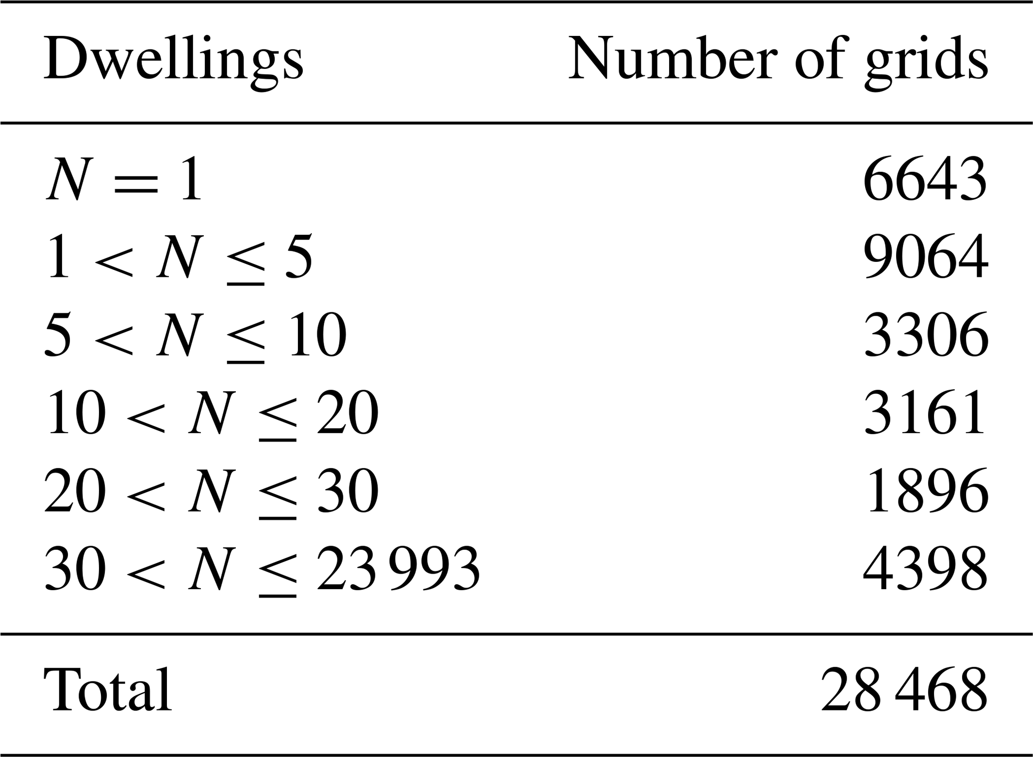
The dataset underlying the EIRM represents a huge amount of work. At the time of writing (end of 2018), 32 countries (EU and non-EU member states alike) had contributed data, and information from almost 1.2 million dwellings has been aggregated into 28 468 grid cells. Since some cells overlap between countries, 28 203 of these grid cells were filled by one country, while 262 and 3 grids were filled by two and three countries, respectively (i.e. border areas which share the same grid) (version: 29-09-2018). However, there is still a large number of grid cells over European territory with no data, and the number of measurements per grid cell varies widely, from many with only one measurement up to a single one with 23 993 dwellings sampled (Table 1). Evaluating the radon exposure to European citizens would therefore require another 10 years, or more, if it had to be done based on indoor radon measurements over each grid cell.

Table 1 Number of dwellings sampled by grid cells of 10 km × 10 km in the study area.

Interpolation techniques are therefore essential at this stage to predict a mean indoor radon concentration in the grid cells for which no or few data are available, and thus develop a Pan-European Indoor Radon Map. We have tested four interpolation techniques: two that use solely indoor radon concentration measurements, viz. inverse distance weighting (IDW) and ordinary kriging (OK), and another two which also take into account geological information, viz. collocated cokriging with the uranium concentration in topsoil as a secondary variable (CCK) and regression kriging with topsoil geochemistry and bedrock geology as secondary variables (RK). Cross-validation exercises were carried out to assess the uncertainties associated with each method. The map generated here is a hypothetical indoor Rn map in the sense that it estimates the mean per 10 km × 10 km grid cell under the assumption that there are dwellings in the grid cell. In some remote areas (mountains, extreme northern Europe), however, this may not be the case in reality. The final map represents a first step towards a European radon exposure and, further on, a radon dose map. Furthermore, it may assist European countries in developing their respective national indoor radon maps.

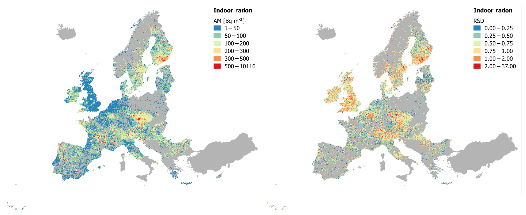
Figure 1 Arithmetic mean (AM_z) over 10 km × 10 km grid cells (Bq m⁻³) and relative standard deviation (RSD = AM∕SD).

Figure 2 Histogram and q–q plot of average indoor radon concentration (AM_z) on the ground floor of dwellings.

2 Methods

2.1 Indoor radon data

The primary dataset used to predict the mean per grid cell with no or few data is the one of arithmetic means (AM_z). The AM was assigned to the centre of each grid cell, and predictions were carried out only in grid cells where U, Th, and K₂O concentrations were also available (46 000 grid cells; version 28-05-2018, Pantelić et al., 2018). Data from grid cells filled by more than one country (i.e. points with the same coordinates) were merged and the summary statistics recalculated according to Eqs. (1)–(10).

$$\begin{array}{}\text{(1)}& {\displaystyle }& {\displaystyle }\mathrm{AM}={\displaystyle \frac{S}{N}}\text{(2)}& {\displaystyle }& {\displaystyle }\mathrm{SD}=\sqrt{{\displaystyle \frac{SQ-\frac{s^{\mathrm{2}}}{N}}{N-\mathrm{1}}}}\text{(3)}& {\displaystyle }& {\displaystyle }\mathrm{Med}=\sqrt{\prod _{i=\mathrm{1}}^n{\mathrm{med}}_i}\left(\mathrm{approximation}\right)\text{(4)}& {\displaystyle }& {\displaystyle }\mathrm{Min}=\min \left[{\min }_i\right]\text{(5)}& {\displaystyle }& {\displaystyle }\mathrm{Max}=\max \left[{\max }_i\right]\text{(6)}& {\displaystyle }& {\displaystyle }N=\sum _{i=\mathrm{1}}^n{N}_i\end{array}$$

$$\begin{array}{}\text{(7)}& {\displaystyle }& {\displaystyle }S=\sum _{i=\mathrm{1}}^n{S}_i\text{(8)}& {\displaystyle }& {\displaystyle }{S}_i={\mathrm{AM}}_i\cdot N_i\text{(9)}& {\displaystyle }& {\displaystyle }SQ=\sum _{i=\mathrm{1}}^{n}S{Q}_i\text{(10)}& {\displaystyle }& {\displaystyle }S{Q}_i={\mathrm{SD}}_i\cdot \left(N_i-\mathrm{1}\right)+{\displaystyle \frac{S_i}{N_i}}\end{array}$$

Here “i” is the number of countries that filled the grid. The values for the log-transformed data (AM_lnz and the SD_lnz) were estimated with the same equations as used for the AM and the SD, but with the ln values provided by each country (i.e. AM_lnz and SD_lnz).

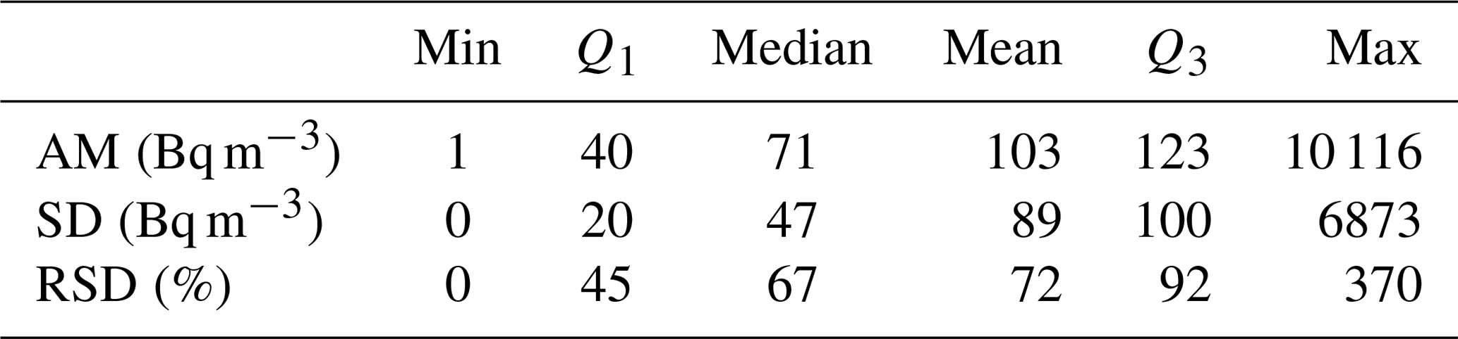
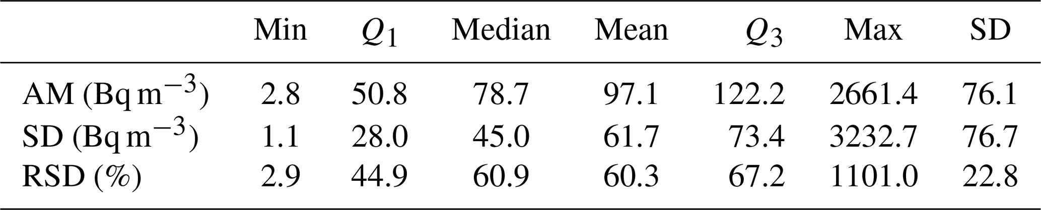
In the study area (i.e. area with topsoil geochemistry data) there are 25 367 grid cells with indoor radon measurements (Fig. 1). The distribution of the AM is approximately log-normal (Fig. 2), with values ranging from 1 to 10 116 Bq m⁻³. The summary statistics are shown in Table 2. Nominal concentrations below 10 Bq m⁻³ are unrealistic from the point of view of true occurrence and measurement possibility, but this could not be verified in this context. The impact of such errors on the result is probably negligible.

Table 2 Summary statistics of indoor radon data (AM_z) after merged border grids (N=25 367).

2.2 Interpolation techniques

A mean (over a 10 km × 10 km grid cell) radon concentration at the ground-floor level was estimated at 1 m off the grid centroid, to which the AMs in the input database are referenced. Predictions were therefore carried out at locations slightly different from the ones of the data. The reason is that we wanted to avoid exact interpolations. To some extent, indoor radon variations at a small scale can be taken into account this way.

2.2.1 Inverse distance weighted (IDW) interpolation

The inverse distance weighting (IDW) interpolation technique estimates a weighted average at an unsampled point (${\widehat{Z}}_{\mathrm{0}}$) according to its distance (d_i) to the sampled points (Z_i):

$$\begin{array}{}\text{(11)}& {\widehat{Z}}_{\mathrm{0}}={\displaystyle \frac{\sum _{i=\mathrm{1}}^n\frac{\mathrm{1}}{d_i^{\mathrm{p}}}{Z}_i}{\sum _{i=\mathrm{1}}^n\frac{\mathrm{1}}{d_i^{\mathrm{p}}}}}\mathrm{if}{d}_i>\mathrm{0};\mathrm{otherwise}\left(d_i=\mathrm{0}\right):{\widehat{Z}}_{\mathrm{0}}=Z_i,\end{array}$$

where “p” is the inverse distance weighting power (idp), which represents “the degree to which the nearer points are preferred over more distant points” (Bivand et al., 2008). IDW assumes that, on average, nearby points are more similar to each other than more distant points (Li and Heap, 2008), and therefore the weights for the closer ones are higher than the weights for distant points.

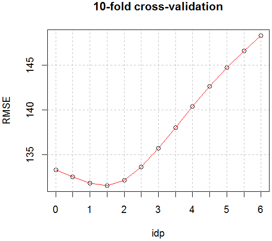
The result is highly influenced by the inverse distance weighting power chosen. An optimal value of p which minimizes a loss function L, p_opt = argmin L (data, target locations; p), can be found for example by k-fold cross-validation. The loss function has to be defined by the user, and a common choice is the root-mean-square error (RMSE) (Janik et al., 2018). In our case the optimal idp was found to be 1.5 (Fig. 3), and interpolations of the AM were carried out using the observations within a distance of 1000 km, and a minimum and maximum number of nearest observations were set to 5 and 75, respectively.

Figure 3 Inverse distance weighting power (idp) optimization.

2.2.2 Ordinary kriging (OK)

Trans-Gaussian kriging using Box–Cox transforms (function krigeTg in R software, packages “gstat” and “MASS”; Gräler et al., 2016; Kendall et al., 2016; Pebesma, 2004; R Core Team, 2018; Venables and Ripley, 2002) was performed with the arithmetic mean. The normal transformation of data (X) with the transformation parameter lambda (λ) follow Eq. (12) (Box and Cox, 1964):

$$\begin{array}{}\text{(12)}& {\mathit{\varphi }}_{\mathit{\lambda }}^{-\mathrm{1}}=\left\{\begin{array}{ll}\frac{X^{\mathit{\lambda }}-\mathrm{1}}{\mathit{\lambda }}& \mathit{\lambda }\ne \mathrm{0}\\ \log \left(X\right)& \mathit{\lambda }=\mathrm{0}\end{array}\right..\end{array}$$

Predictions are carried out over the transformed data and then unbiased back-transformed to the original scale using the Lagrange multiplier (Eqs. 13–15; Cressie, 1993; Varouchakis et al., 2012):

$$\begin{array}{}\text{(13)}& {\displaystyle }& {\displaystyle }\widehat{Z}\left(S_{\mathrm{0}}\right)=\mathit{\varphi }\left({\widehat{Y}}_{\mathrm{OK}}\left(S_{\mathrm{0}}\right)\right)+{\mathit{\varphi }}^{\prime \prime }\left(\widehat{\mathit{\mu }}\right)\left({\displaystyle \frac{{\mathit{\sigma }}_{\mathrm{OK}}^{\mathrm{2}}\left(S_{\mathrm{0}}\right)}{\mathrm{2}}}-m\right),\text{(14)}& {\displaystyle }& {\displaystyle }\mathit{\varphi }\left(x\right)=\left\{\begin{array}{ll}(x\cdot \mathit{\lambda }{)}^{\frac{\mathrm{1}}{\mathit{\lambda }}}& \mathit{\lambda }\ne \mathrm{0}\\ e^x& \mathit{\lambda }=\mathrm{0}\end{array}\right.,\text{(15)}& {\displaystyle }& {\displaystyle }{\mathit{\varphi }}^{\prime \prime }\left(x\right)=\left\{\begin{array}{ll}(\mathrm{1}-\mathit{\lambda })(x\cdot \mathit{\lambda }+\mathrm{1}{)}^{\frac{\mathrm{1}}{\mathit{\lambda }}-\mathrm{2}}& \mathit{\lambda }\ne \mathrm{0}\\ e^x& \mathit{\lambda }=\mathrm{0}\end{array}\right.,\end{array}$$

where $\widehat{Z}(S_{\mathrm{0}}$) is the ordinary kriging predictor on the original scale, ${\widehat{Y}}_{\mathrm{OK}}\left(S_{\mathrm{0}}\right)$ the ordinary kriging predictor on the transformed scale data, ${\mathit{\sigma }}_{\mathrm{OK}}^{\mathrm{2}}\left(S_{\mathrm{0}}\right)$ the ordinary kriging variance, $\widehat{\mathit{\mu }}$ the mean estimate at each location, and m the Lagrange multiplier of the OK system for each location (Kozintsev et al., 1999).

The variogram was modelled with two components: a Matérn model (Minasny and McBratney, 2005; Pardo-Iguzquiza and Chica-Olmo, 2008) up to a distance of 50 km and an exponential model up to 1500 km (Fig. 4). The very low kappa (0.15) points to high “roughness” of the field. Predictions were then carried out with observations within a distance of 1000 km and using a minimum and a maximum number of nearest observations of 5 and 75, respectively.

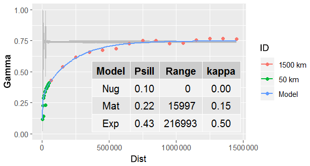
Figure 4 Model variogram (blue line; green dots are pairs of points up to a distance of 50 km and red points up to 1500 km) and 100 variograms from random permutations of the data (grey lines).

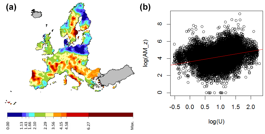
Figure 5 (a) Uranium concentration in topsoil (max = 9.73 mg km⁻¹; Tollefsen et al., 2016) and (b) scatterplot between indoor radon and uranium concentration in topsoil.

2.2.3 Collocated cokriging (CCK) with uranium as secondary variable

Collocated cokriging (CCK) is a special case of cokriging where only the direct correlation between the primary (e.g. AM_z) and the secondary variables (e.g. U) is used, ignoring the direct variogram of the secondary variable and the cross variograms. It simplified the cokriging equations although the secondary variable must be sampled at all prediction points (Bivand et al., 2008). The method is a simplification of the physical reality because the dependence structure between covariates is more complex, as they result from different physical processes.

We performed the CCK with the uranium concentration in topsoil as a secondary variable since radon is generated in the uranium decay series (Cothern and Smith, 1987), and a positive correlation between uranium and indoor radon is therefore expected. The analysis was carried out with the data log-transformed and then back-transformed to the original scale (AM_z) with Eqs. (16) and (17) (where μ is the kriging prediction and σ the kriging variance):

$$\begin{array}{}\text{(16)}& {\displaystyle }& {\displaystyle }E\left[X\right]=e^{\left(\mathit{\mu }+\frac{{\mathit{\sigma }}^{\mathrm{2}}}{\mathrm{2}}\right)},\text{(17)}& {\displaystyle }& {\displaystyle }\mathrm{var}\left[X\right]=e^{\left(\mathrm{2}\mathit{\mu }+{\mathit{\sigma }}^{\mathrm{2}}\right)}\cdot \left(e^{{\mathit{\sigma }}^{\mathrm{2}}}-\mathrm{1}\right).\end{array}$$

The uranium map (Fig. 5a; Tollefsen et al., 2016), part of the European Atlas of Natural Radiation, has been created using approximately 5000 topsoil data from the GEMAS and FOREGS datasets (i.e. GEMAS: Geochemical Mapping of Agricultural and Grazing Land soil in Europe, GEMAS, 2008; and FOREGS: Geochemical Atlas of Europe developed by the Forum of European Geological Surveys, FOREGS, 2005). Uranium explains about 7.75 % of the total indoor radon variability (correlation coefficient = 0.2783; Fig. 5b). As in the previous cases, a maximum distance of 1000 km and a minimum and maximum number of nearest observations of to 5 and 75, respectively, were used in the predictions.

2.2.4 Regression kriging (RK)

Regression kriging (RK) is a two-step interpolation technique: first, a regression estimation of the dependent variable (e.g. AM_z) is performed against secondary variables (e.g. geogenic factors), and, second, an analysis of the spatial distribution of the residual is carried out using geostatistical methods (i.e. OK; Pásztor et al., 2016). The final estimates are the sums of the regression estimates and the ordinary kriging estimates of the residuals (Di Piazza et al., 2015). The analysis was also carried out with the log-transformed data and directly back-transformed with the same equation as in CCK.

The technique applied in the regression step can vary (Li and Heap, 2008); here, we have performed a linear regression using topsoil geochemistry (i.e. U and K₂O) and geology (i.e. 1:5 Million International Geological Map of Europe – IGME 5000; Asch, 2003) as secondary variables. The IGME 5000 has been developed by the German Federal Institute for Geosciences and Natural Resources; this European GIS project involved more than 40 European and adjacent countries, covering an area from the Caspian Sea in the east, to the mid-ocean ridge in the west, and from Svalbard Islands in the north to the southern shore of the Mediterranean Sea. The aim of the project was to develop a GIS underpinned by a geological database. The original IGME map presents 178 lithostratigraphic units that were reduced to 28 lithological units (Fig. 6). Based on ANOVA tests ran on an extensive Italian geological database, Nogarotto et al. (2018) demonstrated that lithology alone has a large effect on geochemical variations in key elements (U, Th, K₂O), regardless of the tectonostratigraphic position of a given unit. It is therefore assigned the prevalence unit to each grid of 10 km × 10 km (Fig. 6).

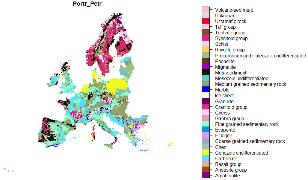
Figure 6 Simplified geology map with geological units defined on a lithology basis (Nogarotto et al., 2018). The base geological map is the IGME (Asch, 2003).

Figure 7 (a) Linear model and (b) variogram of residuals.

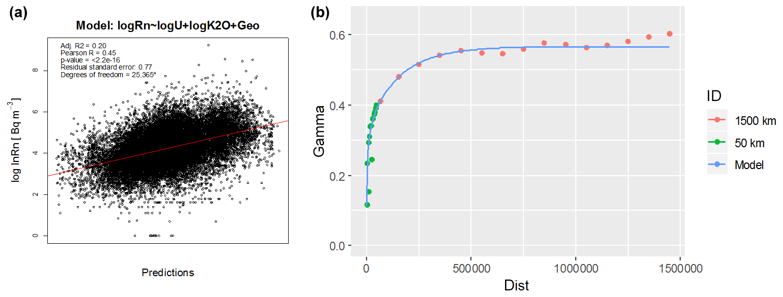
The procedure is therefore (i) to fit a linear model to the data (Fig. 7a and Table 3), where the total indoor radon variance explained by U, K₂O, and simplified geology is 20.24 % (7.75 %, 7.88 %, and 4.61 %, respectively); (ii) to analyse the spatial distribution of residuals, ordinary kriging (Fig. 7b); (iii) to predict a radon value (i.e. log(AM_z)) in each grid using the linear model and add the residual predictions; and iv) to back-transform to the original scale with the equations described in the previous section (Eqs. 16 and 17; where μ is the linear model prediction plus the ordinary kriging prediction of the residuals, and σ is the kriging variance).

Table 3 ANOVA table for indoor radon concentration.

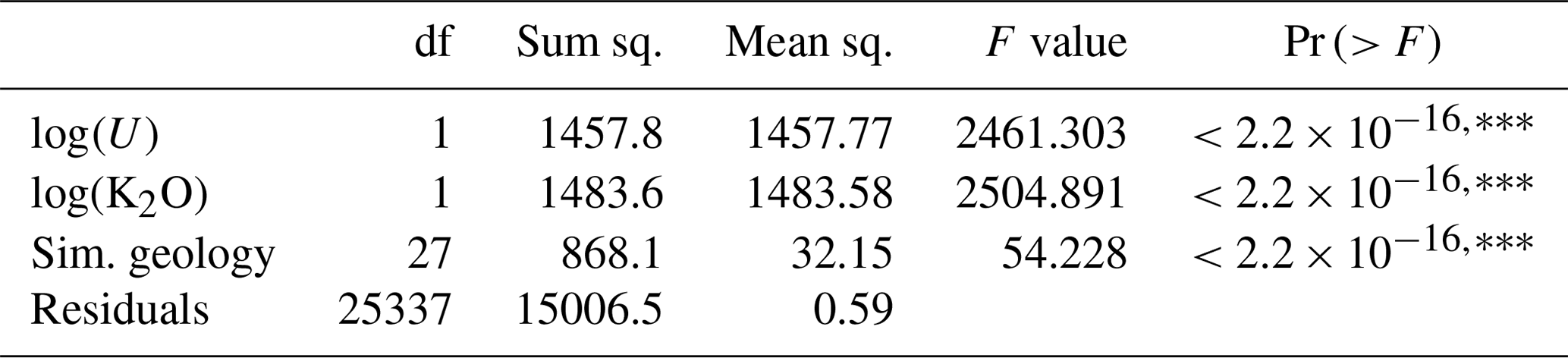
Significance codes: ${}^{***}$ denotes p values < 0.001; ${}^{**}$ denotes p values < 0.01; ^* denotes p values < 0.05; a full stop denotes p values < 0.1; and for p values > 0.1 nothing is printed.

2.2.5 Cross-validation

The performances of the different methods were assessed by 5×10-fold cross-validation and by moving-window cross-validation (Kasemsumran et al., 2006). For the 5×10-fold cross-validation method, data were randomly split into 10 subgroups and predictions were carried out 10 times; each time one group is used for validation and nine are used for modelling the variable of interest (i.e. AM_z) at the validation locations. This process is then repeated five times, obtaining a total of 50 realizations. The moving-window cross-validation (MWCV) was carried out with cell sizes of 200 km × 200 km (total number of windows = 197). Grid cells within a window are removed, and an AM is predicted with the rest, then errors are calculated and the process is repeated with another window until all windows are covered. Some restrictions to the validation set were used to avoid errors during kriging methods (i.e. number of grids in the validation set higher than 1; var(log[U]) > 0; and geological units of the validation set must also be in the model set).

The accuracy of the different methods was assessed using six indicators: the mean absolute error (MAE), the root-mean-square error (RMSE), the root-mean-square log error (RMSLE), the index of agreement (IA), the percentage bias (PB), and the coefficient of determination (R²) (Eqs. 18–23).

$$\begin{array}{}\text{(18)}& {\displaystyle }& {\displaystyle }\mathrm{MAE}={\displaystyle \frac{\mathrm{1}}{n}}\sum _{i=\mathrm{1}}^n\left|Z_i-X_i\right|\text{(19)}& {\displaystyle }& {\displaystyle }\mathrm{RMSE}=\sqrt{{\displaystyle \frac{\mathrm{1}}{n}}\sum _{i=\mathrm{1}}^n{\left(Z_i-X_i\right)}^{\mathrm{2}}}\text{(20)}& {\displaystyle }& {\displaystyle }\mathrm{RMSLE}={\displaystyle \frac{\mathrm{1}}{n}}\sum _{i=\mathrm{1}}^n{\left(\log \left(Z_i+\mathrm{1}\right)-\log \left(X_i+\mathrm{1}\right)\right)}^{\mathrm{2}}\end{array}$$

$$\begin{array}{}\text{(21)}& {\displaystyle }& {\displaystyle }\mathrm{IA}=\mathrm{1}-{\displaystyle \frac{\sum _{i=\mathrm{1}}^n{\left(Z_i-X_i\right)}^{\mathrm{2}}}{\sum _{i=\mathrm{1}}^n{\left(\left|X_i-\stackrel{\mathrm{‾}}{X}\right|-\left|Z_i-\stackrel{\mathrm{‾}}{X}\right|\right)}^{\mathrm{2}}}}\text{(22)}& {\displaystyle }& {\displaystyle }\mathrm{PB}=\mathrm{100}{\displaystyle \frac{\sum _{i=\mathrm{1}}^n\left(Z_i-X_i\right)}{\sum _{i=\mathrm{1}}^n{X}_i}}\text{(23)}& {\displaystyle }& {\displaystyle }{R}^{\mathrm{2}}=\mathrm{1}-{\displaystyle \frac{\sum _{i=\mathrm{1}}^n{\left(Z_i-X_i\right)}^{\mathrm{2}}}{\sum _{i=\mathrm{1}}^n{\left(X_i-\stackrel{\mathrm{‾}}{X}\right)}^{\mathrm{2}}}}\end{array}$$

Here Z_i and X_i are the predicted and measured values in the validation location (S_i), n the number of points in the validation group, and $\stackrel{\mathrm{‾}}{X}$ the mean of X_i. MAE and RMSE are commonly used for assessing model performance; however, they may be influenced by outliers (Chen et al., 2017). RMSLE, on the contrary, is less sensitive to outliers and preferable when there is a large range in the values (Janik et al., 2018). These parameters are positive values, and the closer they are to 0, the better the model fit is. IA is a standardized measure of the degree of model prediction error; it varies from 0 (no agreement at all) to 1 (perfect match). PB (%) measures the average tendency of having larger/smaller predicted values than the observed ones. The optimal value is 0, and positive/negative values indicate over/underestimation bias (Janik et al., 2018). Finally, R² is a measure of how well the model fits a dataset; a perfect model has R²=1 (Alexander et al., 2015).

3 Results and discussion

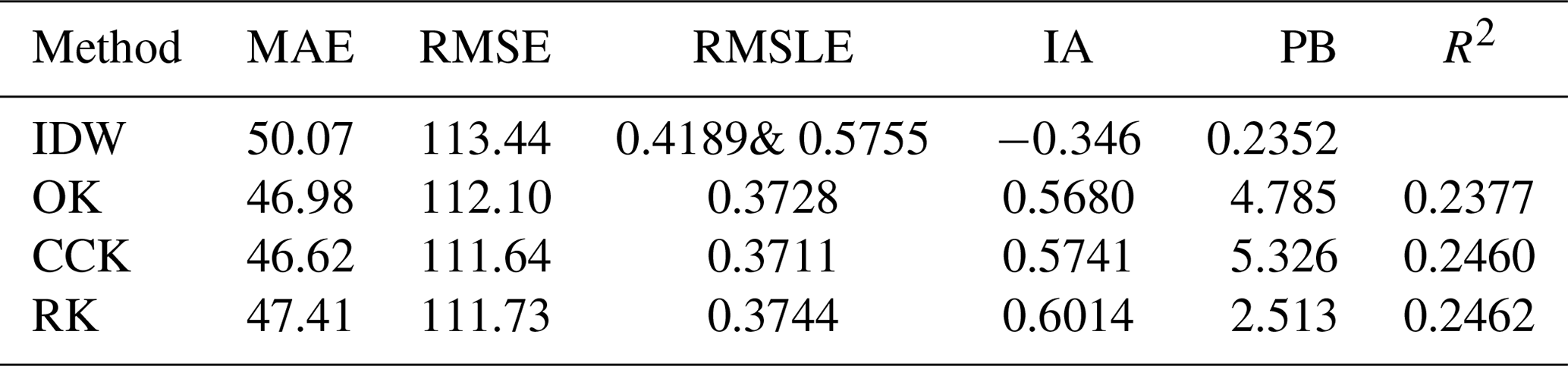
3.1 Cross-validation

The 5×10-fold cross-validation (Fig. 8 and Table 4) shows that geostatistical techniques (i.e. OK, CCK, RK), which take into account the spatial autocorrelation of the data, generally perform better (i.e. lower MAE and RMSLE and higher R²) than IDW. However, they have a tendency to overestimate bias (PB > 0). Then, geostatistical results are slightly improved when geological information is added. The model which has the highest R² is RK (median = 0.2462), followed by CCK (0.2460) and OK (0.2377). RK is also the geostatistical technique with higher IA (0.6014) and lower PB (2.513), and it has similar MAE and RMSLE as OK and CCK (around 47 and 0.36, respectively).

Figure 8 Box plot of the 5×10-fold cross-validation results.

Table 4 The 5×10-fold cross-validation results.

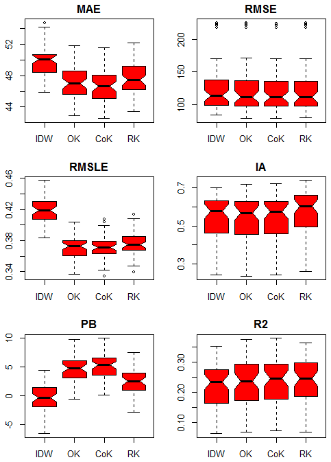
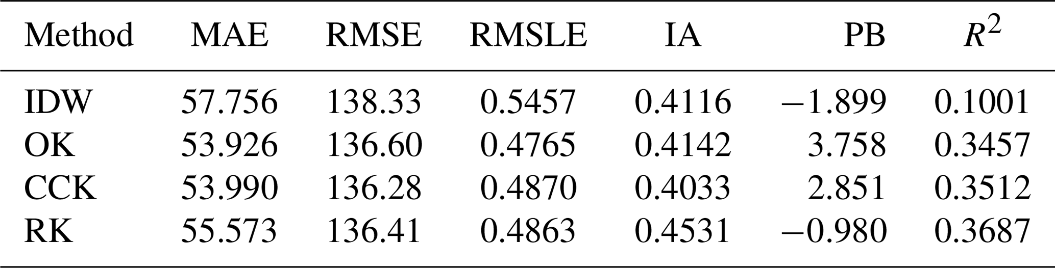
Similar results are obtained in the MWCV exercise (Table 5). Geostatistical techniques (i.e. OK, CCK, RK) also have the highest R² and the lowest MAE and RMSLE. However, in these cases the RK bias is close to 0 (PB = −0.98), while OK and CCK overestimate the values. MWCV also suggests that results are slightly improved when geogenic factors are taken into account: e.g. R² increases from 0.3457 (OK) to 0.3512 (CCK) and then to 0.3687 (RK); and the highest IA is obtained with RK (0.4531). However, similar MA, RMSE, and RMSLE were also found (around 54, 136, and 0.48, respectively), which indicates the difficulty of predicting an average indoor radon concentration even when secondary variables are added.

Table 5 Moving-window cross-validation results.

3.2 Indoor radon predictions

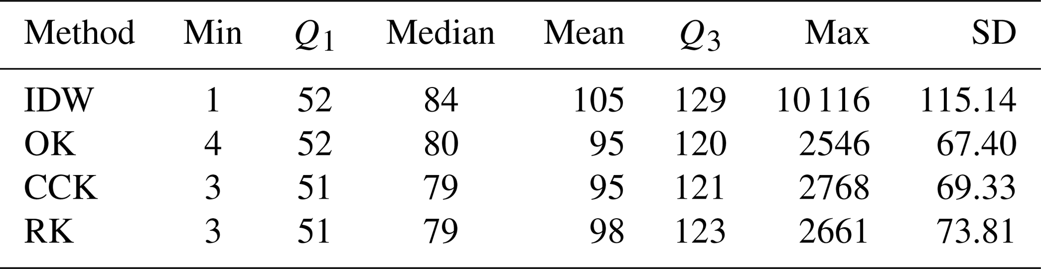
Radon predictions with the different methods range from minimum values of 1–4 Bq m⁻³ to up to 10 116 Bq m⁻³, while the mean values are of the order of 95–105 Bq m⁻³ (Table 6). The very high value of an AM (i.e. 10 116 Bq m⁻³) seems improbable, although the grid is in a region with uranium deposits and former uranium mines (border region between Spain and Portugal). This cell has only two measurements (i.e. 9726 and 10 507 Bq m⁻³), so that the level of reliability of this extremely high AM is therefore low and it would probably decrease if the number of data were increased. In this sense, IDW interpolation, which gives an exact interpolation when the distance between the predicted and measured points is zero, estimates a value that is the arithmetic mean (i.e. 10 116 Bq m⁻³). Nevertheless, when the spatial autocorrelation between cells is considered (i.e. OK, CCK, and RK), the predicted values, although also high, are reduced to 2500–2800 Bq m⁻³. These latter values may be more realistic and are similar to average values found in some villages of the region (i.e. 1851 Bq m⁻³ in Villar de la Yegua, Spain; Sainz et al.. 2010). However, this effect shows the difficulties with predicting an AM when the number of measurements in a grid cell is low. Geostatistical techniques may help to overcome some of these limitations, although the reliability of data because of different numbers of measurements (e.g. grids with only one or two and others with more than 20–30 measurements) is still a problem. It is also not clear whether in an “anomalous area” such as the one cited above, where the geological conditions are particular, the covariance function (or the variogram), which has been estimated from all data, still applies. One can assume that in such a region 2nd-order stationarity is violated. But the accuracy of local prediction depends very much on the local covariance model.

Table 6 Summary of indoor radon predictions (AM, ground floor).

Small differences may be appreciated in the predictions of the different interpolation techniques (Fig. 9). IDW and OK are methods that rely on the Rn data only, while CCK and RK use additional predictors (i.e. geology, U and K₂O concentration in the ground) as secondary variables. The first type is weak in areas with no conditioning data as it simply interpolates between existing ones, ignoring physical reality in these areas (e.g. south Italy, north-east Germany). Including it is the rationale of the second type; practically, missing conditioning data of the primary variable (Rn) are substituted by functions of the secondary variables. Although certainly more reasonable in the physical sense, this type is analytically more complicated.

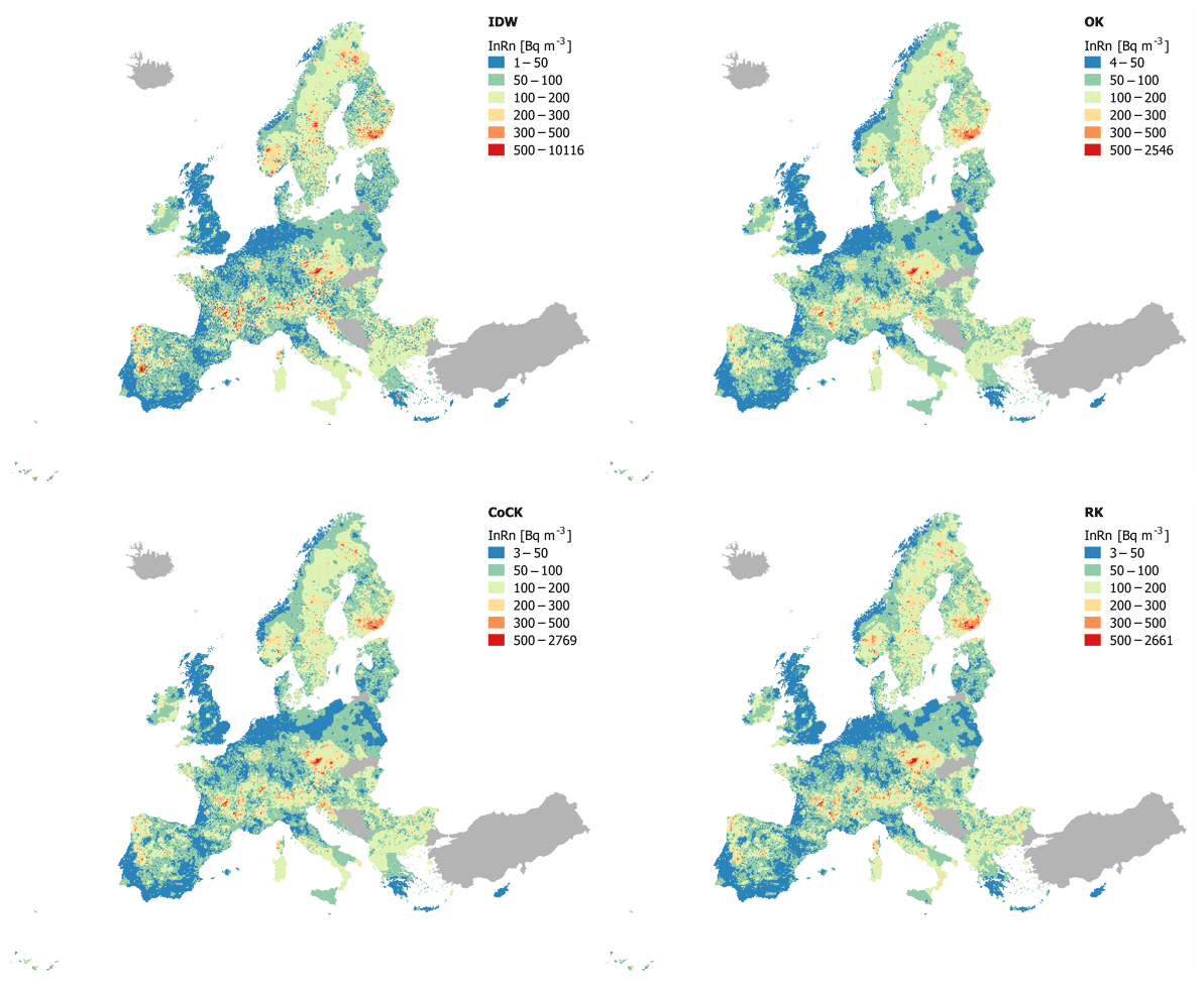
Figure 9 Indoor radon predictions (AM (Bq m⁻³), ground floor).

The influence of geogenic factors on indoor radon is well known and normally used for radon mapping (e.g. Casey et al., 2015; Elío et al., 2017; Pásztor et al., 2016; Scheib et al., 2013; Tondeur et al., 2014). In our cases, an ANOVA (Table 3) shows that the total indoor radon variance explained by U, K₂O, and geology is about 20 % (7.75 %, 7.88 %, and 4.61 %, respectively). Uranium is a source of radon in soil, and thus a positive association with indoor radon is expected (e.g. Appleton et al., 2008; Ferreira et al., 2018). However, the Pearson's correlation coefficient between indoor radon and uranium concentration in topsoil is relatively low (r=0.2783), which implies that CCK estimations with U as the secondary variable are still mainly based on the primary variable (i.e. AM; Rocha et al., 2012). Therefore, although CCK performs slightly better than OK, spatial predictions are similar (Fig. 9).

Geology is associated with both uranium and radon sources and with physical properties which permit the release of radon from the soil matrix and its transport in the environment (e.g. mineralogy, porosity, permeability). The total indoor radon variance explained by geology is normally of the order of 5 %–25 % (Appleton and Miles, 2010; Borgoni et al., 2014; Miles and Appleton, 2005; Tondeur et al., 2014; Watson et al., 2017), although it depends on the geological scale map (i.e. increase with the scale; Appleton and Miles, 2010). A 4.64% of indoor radon variation explanation is therefore reasonable, taking into account that we used a simplified 1:5 million geological map and that data are averaged over grids of 10 km × 10 km.

The positive correlation between indoor radon and potassium is, however, not evident. K₂O may be related to clay content in soils (e.g. Barré et al., 2008; Milošević et al., 2017; Tarvainen et al., 2005), and although the permeability of wet clays is low, it may increase when soils are dried (Petersell et al., 2005) as a consequence of building a house (Barnet et al., 2008). This hypothesis should be tested since clay soils are normally considered low risk although its radium concentration may be high (Maestre and Iribarren, 2018). We have decided, however, to include this parameter in the model since previous studies have shown a positive association between indoor radon and K₂O/clay (Forkapic et al., 2017).

Table 7 Summary of indoor radon at the European scale.

Back-transforming predictions to the original scale is a critical point of log-normal and trans-Gaussian kriging. OK as given in this study solves this problem by using the Lagrange multiplier in the back-transformation. However, the E[X] and Var[X] for CCK and RK are biased, unless the true mean is known (although for RK it should be zero by definition). These equations should also use the Lagrange multiplier which appears in the kriging system (Chilès and Delfiner, 1999; Matheron, 1974); but unfortunately in common geostatistical packages this parameter is not accessible, and it is not easy to estimate it. Another problem with log-normal kriging is that ill assessment of the kriging SD leads to large errors in E[X] and Var[X] due to exponentiation, so that variogram parameters must be estimated very carefully (Armstrong and Boufassa, 1988). Deviations from stationarity and uni- as well as multivariate log-normality are also critical (Cressie, 1993; Roth, 1998). On the other hand, in highly skewed quantities (as is typical for Rn and in fact for many positive-definite environmental quantities such as concentrations) there seems to be little choice but to work with transformed (e.g. log, Box–Cox, N score) variables.

Finally, a theoretical problem, if using kriging-type interpolators, it may be that input data are actually cell or grid means (blocks in geostatistical language), treated as point samples. The change-of-support problem, which is particularly unpleasant in log-normal kriging, may be alleviated since the target supports are also the same. We regard input data as point data at the cell centre, and we estimate points at other locations that again represent cells of the same size. However, the theoretical aspect remains to be clarified in more depth. Taking into account all of these limitations and weaknesses, the solution demonstrated here, however, represents an acceptable compromise between mathematical exactness, numerical tractability, and complexity of the physical realm.

4 A pan-European indoor radon map

We would like to produce the Pan-European Indoor Radon Map by minimizing data processing, and therefore we prefer to estimate the radon average directly by indoor radon measurements carried out at each grid (i.e. AM_z). However, if the number of measurements were low, the uncertainty of this value could be high. In this sense, if dwellings were randomly selected and therefore representative, which is the condition for unbiased estimates of the mean and other statistics, and the sample size large, the mean value and the confidence interval would be (Eq. 24)

$$\begin{array}{}\text{(24)}& \stackrel{\mathrm{‾}}{x}={\displaystyle \frac{\mathrm{1}}{n}}\sum _i^n{x}_i\pm t_{\left(\mathrm{1}-\frac{\mathit{\alpha }}{\mathrm{2}},n-\mathrm{1}\right)}{\displaystyle \frac{s}{\sqrt{n}}}.\end{array}$$

An additional condition for the validity of the confidence interval is statistical independence of the data. For large n, due to the central limit theorem, $t_{\mathrm{1}-\mathit{\alpha }/\mathrm{2};n-\mathrm{1}}$ can be approximated by the normal score $x_{\mathrm{1}-\mathit{\alpha }/\mathrm{2}}$.

The confidence interval decreases when the sample size increases. In our cases (Fig. 10), the relative (to the mean) CI_95 % (α=0.05) for sample size of about 30–40 data is around ±5 % and generally lower than 15 %–30 %. Therefore, although the assumption of data independence is not valid (i.e. there is spatial correlation between indoor radon measurements which can be modelled by the variogram), 30 measurements seems reasonable for obtaining a good estimation of the radon exposure in a specific grid (Fig. 11). However, if sampled dwellings were highly clustered, the AM could be not representative of the radon exposure in a grid even with high numbers of indoor radon measurements.

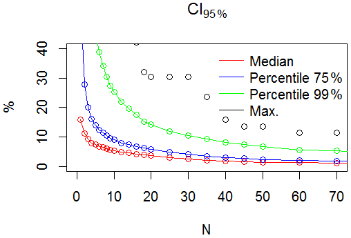
Figure 10 Variation in the 95 % confidence interval of the arithmetic mean according to the sample size (N).

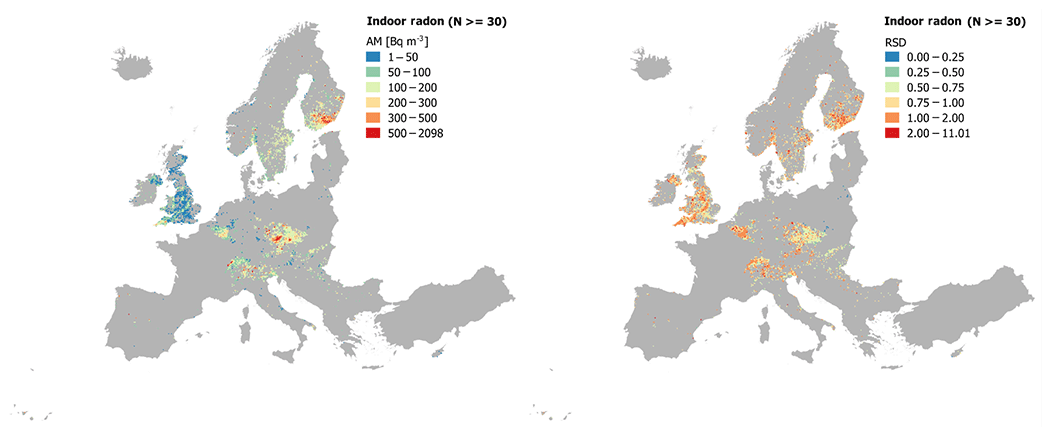
Figure 11 Grids with 30, or more, indoor radon measurements (N=4173; AM: arithmetic mean in becquerels per cubic metre; RSD: relative standard deviation in percent).

For the final Pan-European Indoor Radon Map (Table 7 and Fig. 12), we therefore use the AM of the grid cells with 30 or more measurements (Fig. 11) and the value predicted by RK (Fig. 9) in the cells with fewer than 30 measurements. Indoor radon concentration ranges from 3 to 2662 Bq m⁻³, with a mean value of 98 Bq m⁻³. The standard deviation may be calculated with the SD of the measurements carried out in the grids with 30 or more data and with the kriging standard deviation of the RK (i.e. grids with fewer than 30 measurements). It ranges from 1 to 3233 Bq m⁻³, with a RSD from 3 % to up to 1101 %. The map appears “noisy” to varying degrees between different regions. The reason is that in regions with more conditioning, Rn data, local variability of the estimate is higher than in regions with sparse or without data, where the estimate is based essentially on geology and geochemistry. These covariates are much smoother on the scale available to us than Rn data, where available. Were we to dispose of denser geochemical data and higher-resolution geological maps, these regions would also appear noisier.

Figure 12 Final Pan-European Indoor Radon Map.

5 Conclusions

After more than 10 years of collecting and processing Rn data, with the support of 32 European countries, we could cover approximately 50 % of the continent with 10 km × 10 km grids containing the mean indoor radon concentration in ground floors of dwellings. However, completing the European Indoor Radon Map still requires a significant effort by the participating countries since a robust estimation of the radon exposure in a grid of 10 km × 10 km involves at least 30 indoor radon measurements and, at the time of writing this article, most of the grids cells sampled (78 %) have fewer than 20 dwellings tested. Interpolation techniques which take advantage of the contiguity of Rn seen as a spatially random field may help to overcome some of the present limitations and would permit estimation of radon exposure at the European scale until the coverage of all of Europe with indoor radon measurements has strongly improved.

Of the four methods tested in this study, regression kriging (RK), using a simplified geological map and the topsoil concentration of U and K₂O, has proven to be the best one for predicting mean indoor radon concentrations over grids of 10 km × 10 km (i.e. arithmetic mean, ground floor). By combining RK predictions with empirical average values (AM) in grids with 30 or more measurements, a Pan-Europe Indoor Radon Map has been created. The map represents the average value of indoor radon concentration on the ground floor, and thus it is not representative of the radon exposure to European citizens since most people do not live on the ground floor (Cinelli et al., 2019). However, it is the first step towards a radon exposure map and, in the future, a dose map. Based on demographic and sociological databases, we plan to develop models which allow correction from ground-floor dwellings to the real situation, accounting for the building stock (Bossew et al., 2018).

The Pan-European Indoor Radon Map is not a finished map, and it will be upgraded as new data become available. In future versions a larger scale of the geological map (e.g. scale 1:1 million), as well as other geogenic factors which may influence the indoor radon concentration (e.g. soil units, aquifer types), would be included in the model. Furthermore, the influence of anthropogenic factors and those which may affect building characteristics and living styles (e.g. average temperatures, annual precipitation, altitude) will be analysed. Finally, machine-learning techniques are viewed as promising methods for modelling the AM since kriging-type predictions come to an end if many (intercorrelated) predictors are involved.