the Creative Commons Attribution 4.0 License.
the Creative Commons Attribution 4.0 License.
 | 30 Oct 2019
Numerical modeling using an elastoplastic-adhesive discrete element code for simulating hillslope debris flows and calibration against field experiments
Adel Albaba
Massimiliano Schwarz
Corinna Wendeler
Bernard Loup
Luuk Dorren
This paper presents a discrete-element-based elastoplastic-adhesive model which is adapted and tested for producing hillslope debris flows. The numerical model produces three phases of particle contacts: elastic, plastic and adhesive. A parametric study was conducted investigating the effect of model parameters and inclination angle on flow height, velocity and pressure, in order to define the most sensitive parameters to calibrate. The model capabilities of simulating different types of cohesive granular flows were tested with different ranges of flow velocities and heights. The basic model parameters, the microscopic basal friction (ϕb) and ratio between stiffness parameters , were calibrated using field experiments of hillslope debris flows impacting a pressure-measuring sensor. Simulations of 50 m3 of material were carried out on a channelized surface that is 41 m long and 8 m wide. The calibration process was based on measurements of flow height, flow velocity and the pressure applied to a sensor. Results of the numerical model matched those of the field data in terms of pressure and flow velocity well while less agreement was observed for flow height. Those discrepancies in results were due in part to the deposition of material in the field test, which is not reproducible in the model. Results of best-fit model parameters against selected experimental tests suggested that a link might exist between the model parameters ϕb and and the initial conditions of the tested granular material (bulk density and water and fine contents). The good performance of the model against the full-scale field experiments encourages further investigation by conducting lab-scale experiments with detailed variation in water and fine content to better understand their link to the model's parameters.
- Article
(10838 KB) - Full-text XML
- BibTeX
- EndNote


Worldwide, the growing demand for land to build on has led to the urbanization of mountainous areas. This has increased the importance of studying the different processes of natural hazards that impose danger on residential areas and infrastructure. On steeper slopes in the affected areas, gravity-driven mass movements such as shallow landslides, triggered by intense rainfall or earthquakes, are frequent. In Switzerland, shallow landslides and hillslope debris flows (Fig. 1) are responsible for high infrastructure damage, blockage of important highways, evacuations and deaths yearly (Andres and Badoux, 2018). Moreover, these processes could increase the damage caused by floods by clogging channels and rivers at bridges and passages. Hillslope debris flows are one type of mass movement where shallow landslides transform into an unconfined (unchannelized) flow following heavy rainfalls or earthquakes. They are sometimes referred to as debris avalanches, but unlike the ones described by Hungr et al. (2014), they rarely entrain sediments along their way (Hürlimann et al., 2015). In comparison with channelized debris flows, they tend to have a shorter run-out distance due to their lateral spreading as no confinement exists. Their overall assessment comprises (i) the mechanics of initial slope failure (Jibson, 1995; Schwarz et al., 2010; Olivares and Picarelli, 2003; Klubertanz et al., 2009; Shen et al., 2017), (ii) the transformation from a sliding block into a deformed flowing mass (Iverson et al., 1997; Gabet and Mudd, 2006) and (iii) the kinematics of the flowing mass (velocity, run-out, etc.). While both first aspects have been extensively investigated, the kinematics of hillslope debris flows have rarely been investigated.

Figure 1Aerial photo of several hillslope debris flow events in Switzerland following a severe rainfall event in summer 2005. Source: Federal Office for the Environment (FOEN).
Numerical modeling has been deployed as an effective tool in simulating the behavior of shallow landslides and hillslope debris flows (Hungr, 1995; Montrasio and Valentino, 2016; Ran et al., 2018). For example, the software RAMMS:Hillslope was developed in the Swiss Federal Institute for Forest, Snow and Landscape Research (WSL), based on a momentum balance using a Voellmy rheological model (Voellmy, 1955; Christen et al., 2010; Graf and McArdell, 2011). Another example is the mass-balance-based Flow-R model, which was developed in the University of Lausanne primarily for regional susceptibility assessments of debris flows (Horton et al., 2013). The model was successfully applied to different case studies in various countries with variable data quality. It was also found relevant to assess other natural hazards such as rockfall, snow avalanches and floods. The basic concept of Flow-R was recently implemented and extended in a model developed at the HAFL called M-Flow, which has been tested for modeling hillslope debris flows (Scherer, 2016). The M-Flow model is fairly simple and only accounts for the mass distribution of the flowing mass according to the terrain, without in-depth investigation of the physical aspects of hillslope debris flows. However, the first preliminary tests using M-Flow to reproduce the propagation and impact pressures of real hillslope debris flow events gave promising results.
Discrete element simulations were also used to investigate flowing characteristics and impact pressures of granular flows down inclines (Teufelsbauer et al., 2009, 2011; Albaba et al., 2015; Wu et al., 2016; Shen et al., 2018). Parameters such as flow velocity, flow height and impact pressure were characterized in these simulations at different sections with in-detail investigation. Results of these simulations were often compared to depth-averaged hydrodynamic models concerning the impacting pressure of these flows on rigid barriers (Faug, 2015; Albaba et al., 2018). Moreover, parametric studies investigating the effect of inclination angles of the chute and the barrier on flow behavior and impact pressure were also carried out (Albaba, 2015). Although these simulations agreed well with the proposed theory concerning the impact, they were mainly carried out for dry granular flows with no consideration of fluid presence. Such presence would change the flow characteristics and the time history of its applied pressure (Vollmöller, 2004; Kattel et al., 2018). Other models based on the discrete element method (DEM) accounted for the presence of fluid by coupling a DEM with either a LBM (lattice Boltzmann method) or a CFD (computational fluid dynamics) solver (Leonardi et al., 2016; Ding and Xu, 2018). Such models were promising for theoretical research questions but are computationally expensive for practical use in the daily practice of hillslope debris flow hazard assessment.
In addition to numerical modeling, lab, medium and full-scale experiments were carried out to investigate the flowing mass behavior of debris flows and their impact on rigid objects. For instance, Hürlimann et al. (2015) set up a 7.5 m long experimental chute in which different samples with different grain size distributions, water contents and volumes were tested. It was found that increasing water content, even by a small amount, would greatly increase the run-out distance (exponential relationship). The increase in clay content resulted in a decrease in the run-out distance. In addition, a proportional relationship was observed between the run-out distance and the volume, although the effect was rather small.
An intermediate-scale flume for testing debris flow was built by the United States Geological Survey (USGS) and is 95 m long, 2 m wide and 1.2 m deep (Iverson and LaHusen, 1993). The majority of its length slopes at 31∘ while the remaining part (7 m) gradually flattens to 2.5∘ and it has a loading capacity of 20 m3 of granular material. The flume has been actively used since 1993 for investigating different aspects of debris flow physics.
A full-scale hillslope debris flow experiment was carried out by Bugnion et al. (2012) by measuring the impact of 16 events of 50 m3 in volume on two impact sensors. A 41 m long, 8 m wide channel was constructed on the side of a rock quarry in Switzerland. The advantage of such full-scale investigation is that it allowed for detailed measurements that are usually overlooked in the post-analysis of previous landslides and hillslope debris flows, especially those parameters that are very difficult to estimate for the post-analysis of events, mainly flow height, velocity and impact pressure.
All in all, although advancements have been achieved, the understanding of shallow landslides and hillslope debris flows is still lacking. Assessments of such natural hazards, unlike rockfalls and avalanches, are therefore mostly based on the experience of experts. In order to improve the hazard assessment of shallow landslides, new tools and methods are needed to calculate the disposition, the evolution and the run-out of hillslope debris flows on a slope for different situations (normal situation, severe precipitation, with and without forest cover, etc.).
This paper presents a new computationally efficient DEM that would partially account for the presence of the fluid composed of water and find material, based on the work of Luding (2008). This is achieved through the adhesive aspect of the contact law, which would indirectly take the presence of such fluid into account, as this fluid would increase the cohesion of the flowing mass. The advantage of this new approach is that it accounts for the interaction between solid grains of the flowing mass as well as the effect of fluid between them, all in the same modeling frame (DEM). As a result, modeling 3-D real-scale experiments or back-calculating historical events of granular flows would be computationally possible.
First, the field experimental data that are used to calibrate and validate the DEM are presented. Subsequently, the DEM is described in detail highlighting the key parameters to calibrate. Next, a parametric study is presented investigating the effects of varying the model microscopic parameters in addition to the mean particle diameter (d50) and channel inclination angle (α). A cross comparison between model results and experimental data is then carried out, with a special focus on flow height, flow velocity and the pressure applied by the flow on pressure-measuring sensors. Finally, the main results are discussed and conclusions are drawn.
2.1 Field experiment of hillslope debris flow
A series of full-scale field experiments of hillslope debris flow were carried out between 2008 and 2010 at the Veltheim test site in the Canton Aargau in Switzerland (see Bugnion et al., 2012). The objectives of the experiments were to measure the height and velocity of hillslope debris flows, as well as the pressure. A flexible barrier, which is widely used as a protection measure against many types of mass movements (Volkwein, 2005; Brighenti et al., 2013; Albaba et al., 2017), was installed downslope the channel and was intensively instrumented in order to measure the internal forces and deformations developed in the barrier while being impacted by flows. In total, 16 tests were carried out, of which eight tests consisted of one release while the remaining eight tests consisted of successive releases, where the debris flows were released successively without cleaning the channel. Each release had a constant volume of 50 m3.

2.1.1 Geometry and material used
At Veltheim, a 41 m long, 8 m wide channel was constructed on the side of a rock quarry in Switzerland (Fig. 2). The channel was excavated to the bedrock bottom creating side walls of 1 m. This excavated material was used to prepare the granular flow, which led to slight differences in granular size distribution of tested materials. In addition, different levels of water content were added to the tested material ranging from 14 % to 28 %, which created densities between 1760 and 2110 kg m−3. The channel was instrumented with laser distance sensors at distances of 14 and 26 m from the reservoir gate. In addition, two pressure plates (2 kHz signal capacity) were installed at a distance of 30 m from the reservoir gate with dimensions of 160 mm × 225 mm and 240 mm × 295 mm (with pressure-measuring areas of 0.0144 and 0.04 m2) for the small and large plates, respectively. The tested flow was similar to those of weekly channelized debris flows. Figure 3 shows snapshots of test 10 shortly after release (3 s after release) and after impacting the pressure sensors (6 s after release).

2.1.2 Measured parameters in the experiments
For each released flow, the flow height at sections 1 and 2 was measured using laser sensors. Sections 1 and 2 are located at distances 14 and 26 m, respectively, downstream from the starting reservoir, where distances are measured parallel to the slope as seen in Fig. 2. In addition, with two sensors installed 30 cm apart at section 2, the velocity of the upper flow surface was derived using the discrete correlation function of the two height signals of the two sensors. The mean front velocity at section 2 was back-calculated using data related to flow arrival time and distance at sections 1 and 2. The pressure applied by the flowing material on the small and large plates was also measured and a filtering mechanism was applied. The filtering of pressure values was applied in order to remove oscillations caused by hard contacts due to large grains that impact the sensors. It was applied by replacing each signal value by the mean value over an interval of 0.05 s. In Sect. 3.1, we investigated the possible relationships between those measured parameters (flow velocity and height) in the experiments and water and fine content of released materials. Previous studies of lab-scale experiments of hillslope debris flows showed that increasing water content had the largest positive change of the run-out distance, which might also indicate a possible increase in flowing velocity (Hürlimann et al., 2015). In addition, a negative correlation was observed between clay content and run-out distance. Both of those relations were found to be nonlinear. Run-out analysis is an important aspect of studying hillslope debris flows, but is out of the scope of this study, as it is not considered in the field experiment.
2.2 Discrete element simulations
The numerical simulation in this study was carried out using a discrete element method (DEM). Today the DEM is widely used for modeling granular media (Maurin et al., 2016; Papachristos et al., 2017; Mede et al., 2018). It is particularly efficient for static and dynamic simulation of granular assemblies where medium can be described at a microscopic scale. The method is based on an explicit finite difference scheme proposed by Cundall and Strack (1979). It applies for a collection of discrete bodies interacting with each other, governed by a contact law. Different contact forces can be considered in both the normal and the tangential direction. Calculations alternate between the application of Newton’s second law to particle motion and a force-displacement law for the particle interactions. In comparison with the finite element method (FEM), the DEM makes large displacements between elements easy to simulate and computationally inexpensive, which is useful when dealing with discontinuous problems in granular medium.
Yet Another Discrete Element (YADE) is an extensible open-source framework for DEM-based discrete numerical modeling (Šmilauer et al., 2010). The simulation loop in YADE starts with detecting contacts between particles. Next, the chosen contact law is applied, which results in new positions and velocities of the particles. YADE contains the main components for the application of the DEM, which include Newton's law, time integration algorithms, damping methods, collision detection, data classes (storing information about bodies and interactions) and command OpenGL methods for drawing popular geometries (Šmilauer et al., 2015).
2.2.1 Contact laws
In the numerical scheme, two possible types of interactions can take place. The first interaction type is the particle–wall interaction, which describes the contact between a particle object from the flow and a wall-like object, which could be the chute's base or a rigid barrier in the simulation. This type of interaction is governed in this study by a viscoelastic contact law (Schwager and Poeschel, 2007), which has been frequently used in many previous studies of granular flows down inclines (Teufelsbauer et al., 2011; Albaba et al., 2015; Leonardi et al., 2016). The elastic part of the contact law is represented by a spring, which is connected in parallel to a dashpot representing the viscous damping. The dissipation of energy is partly controlled by this damping particle collision and can be related to the restitution coefficient of granular materials.
The second type of interaction is particle–particle interaction, which describes the contact between a pair of spherical particles that are part of the granular flow. For this interaction, we implemented an elastoplastic-adhesive contact law in the YADE open-source code based on the work of Luding (2008) to simulate the behavior of a cohesive flow. A hysteric force between two interacting particles Fhys in the normal direction is calculated as follows (see also Fig. 4):
where k1, k2 and kc are stiffness parameters for loading, unloading and adhesive phases of contacts, respectively. δ is the overlapping distance in the normal direction between the two particles.
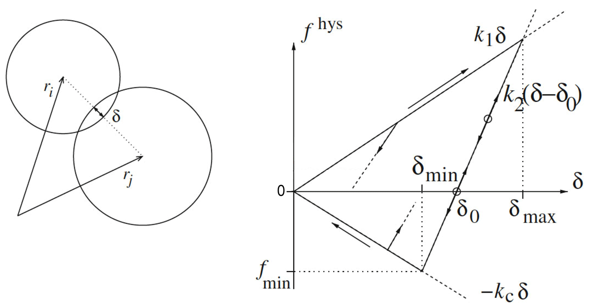
Figure 4A schematic representation of the three phases of the contact law in normal direction.
When a contact between two particles is established, with particles pushing into each other, the hysteric force would start increasing linearly with the increase in the deformation δ along the path of k1. The maximum reached deformation (δmax) will keep being updated as the deformation at the contact increases. Once unloading starts, the reached deformation would be temporarily saved as δmax and the force-deformation path would be followed on the line indicated by the stiffness parameter k2. In case of reloading, the path of k2 would be followed again until reaching the maximum recorded deformation δmax in which further loading would again follow the path of k1. In case of unloading below δ0, which represents the interception between the k2 path and the deformation axis and is calculated as , an adhesive force would be activated, which is limited by the minimum force value .
In addition to the hysteric force component, there is the classical viscous component of the force fvisc (see for information Schwager and Poeschel, 2007), which is the product of the viscous damping coefficient (γn), that depends on the chosen value of the restitution coefficient ϵn (taken equal to 0.3 as indicated by previous DEM studies of granular flows down inclines; Chanut et al., 2010; Albaba et al., 2015), and the velocity in the normal direction (vn), which yields the following form of the interaction force in the normal direction Fn:
The tangential component of the normal force is governed by the classical Mohr–Coulomb failure criterion as follows:
where kt represents the tangential stiffness parameters, ut is the tangential displacement and Φp is the interparticle (microscopic) friction angle.
The normal stiffness of the contact between two particles (k1) is calculated as (Catalano et al., 2014)
where E1 and E2 are the elastic moduli of the first and second particles, respectively (both taken as 108 Pa) and r1 and r2 are the radii of the first and second particles, respectively.
2.2.2 Geometry and chosen parameters
In order to simulate the flow down an inclined chute, a wall object class was used in YADE to create a channel that is made of a base and two side walls. The chute was 41 m long, 8 m wide and channelized with 1 m height sides and inclined at 30∘. At the top of the channel, a rectangular reservoir was created where the flow starts. The reservoir was 7 m long, 8 m wide and 1.8 m high. Inside it, granular samples were created which were made of spherical particles with uniformly distributed diameters ranging from 50 to 100 mm and a mean diameter d50=75 mm. Particles had an intrinsic density ρP=2500 kg m−3. Loose packages of particles were generated at the beginning, with the total volume of each granular sample being around 50 m3. Afterwards, under gravity deposition, particles got deposited at the bottom of the reservoir creating a dense and static sample. Once this step was achieved, the flow simulation starts by opening up part of the reservoir's gate upward for a distance of 0.8 m, thus allowing the particles to flow down the chute (Fig. 5a). Different DEM tests were carried out varying the ratio and the microscopic basal friction angle between particles and the chute's bottom (φb), while fixing the inclination angle α of the chute to 30∘. The interparticle friction φ was 40∘. The tangential stiffness of the contact (kt) was taken as following Silbert et al. (2001) and kc was equal to k1. It is worth noting that the chosen geometrical configurations in DEM simulations corresponded to the those of the field experiment, which were used to calibrate the model (Sect. 2.1).

Figure 5A series of screenshots during a DEM simulation with ϕb=30∘ and : directly after opening the reservoir's gate (a), at t=3.36 s (b), at t=5.92 s (c) and at the end of the simulation (d).
2.2.3 Mechanism of measuring parameters in YADE
Since YADE is a discrete element code, parameters such as height, velocity and pressure were characterized at the particle (micro)scale. In order to present those parameters on a macroscale that is comparable with those of the experimental data, particle-scale parameters needed to be averaged in order to represent the flowing mass as a continuum medium. To compare the simulated mean front velocity with the experiment, the simulated flow arrival time was calculated at positions 1 and 2 and averaged over the distance between those two positions.
The maximum flow height at position 2 is a value that represents the height of the main, coherent flowing body at that position. Firstly, a virtual box was used that was centered at position 2 and had a length 5×d50 and a width and height equal to those of the channel. Flow properties such as position coordinates in x (in the direction of the flow), y (traverse the flow) and z (perpendicular to the base) as well as flowing velocity in the direction of the flow were recorded each 0.1 s for all particles within that box. Secondly, particle height measurements at time periods between 25 % and 75 % of total impact duration were selected for each simulation, in order to exclude the disperse and dilute flow front and flow tail (Jiang and Towhata, 2013; Albaba et al., 2015), such as the ones seen in Fig. 5b. Thirdly, the 90 % cumulative frequency of flow height of particles within the box was selected. The maximum flow height in YADE that is compared to the experiment was then the maximum value of those selected cumulative frequencies for all the samples that were collected each 0.1 s.
For the impacting pressure, a rigid wall in YADE was installed at the same position where the large sensor was installed during the experiments and with the same dimensions (Fig. 5a). Normal force Fn applied to the wall by flowing particles was calculated as follows: , where is the normal force between a particle i and the wall, and n is the number of particles in contact with the wall at that moment. The pressure was then calculated as the ratio between applied force and the sensor's surface area.
2.2.4 Sensitivity analysis of DEM parameters
A sensitivity analysis study was carried out in order to investigate the effect of change of different parameters on the model's results concerning maximum flow height, mean flow front velocity and maximum applied pressure on the large plate. First, the effect of the filtering interval applied to the pressure signal was analyzed in order to use a unified filtering interval for all simulations. Afterwards, the effect of variation in each of the following parameters, ϕb, , kc, d50 and α, was investigated in detail.
2.3 Comparison of DEM and experimental data
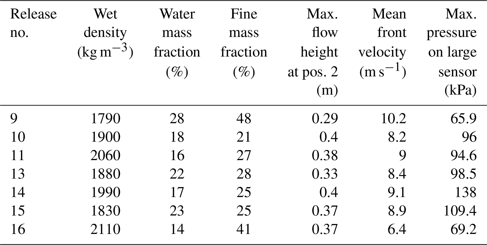
To calibrate the DEM, only first releases of selected tests from the field experiment were considered in order to avoid the possible disturbance of measured parameters in the experiments due to the presence of deposits of previous releases (tests abbreviated as X.1 in Table 4 in Bugnion et al. (2012), where X is the test number). In the current DEM, no material deposited on the inclined plane and thus the multiple releases would be difficult to reproduce. Seven tests from the experimental data were selected to be compared with the DEM results. They are numbered with the same digits as in Bugnion et al. (2012). Table 1 summarizes the main material properties of these tests and the measured parameters.
Table 1Main flow characteristics and measured parameters for experimental tests selected for model calibration.
A series of simulations varying the parameter set (ϕb, ) were carried out. A range between 20 and 40∘ was selected for ϕb with a step-wise increase of 5∘ while was varied between 0.3 and 0.45 with an increment of 0.03. Those ranges were selected based on preliminary model tests. Simulations with ϕb and values that are outside the selected ranges were found to result in either very fast flows with very high impacting pressures or flows that would not slide along the channel. Afterwards, all carried-out simulations were compared with each selected experiment in order to find the best-fit in terms of maximum flow height at position 2 (Hmax), mean front velocity between positions 1 and 2 (Vmean), and maximum applied pressure to the large sensor (Pmax). Results of pressures on smaller sensors were ignored because they were not measured for each test in Bugnion et al. (2012). In addition, in DEM simulations, the smaller the sensor, the more discrete in nature the force signal would be due to the presence of fewer particles per impact. A best-fit for each selected experimental test was determined as the lowest percentage (Rmin) of error for the three parameters as follows:
where ns is the number of simulations.
After finding the best parameter set (ϕb, ) for each experiment, possible relationships between these sets of parameters and initial condition of the granular samples (i.e., water and fine content) were investigated.
3.1 Analysis of experimental data
For the seven selected experimental tests, a relationship seems to exist between the water content in the granular material prepared in the reservoir and the recorded mean front velocity between sections 1 and 2 in the field experiment (Fig. 6). For example, test no. 16 had a water content of 14 % and its recorded mean front velocity was found to be 6.4 m s−1. In addition, water contents between 16 % and 23 % had similar recorded front velocities ranging from 8.2 to 9.1 m s−1 for test numbers 10 to 15. Test no. 9, which had the richest water content, had the highest mean front velocity of 10.2 m s−1. This observed increase in flow velocity with increasing water content could be due to the decrease in basal friction with the flowing material, which leads to higher flowing velocities. However, a best fit of the results might be better represented with a nonlinear equation in comparison with the regression line presented in Fig. 6, which is similar to observations of Hürlimann et al. (2015).
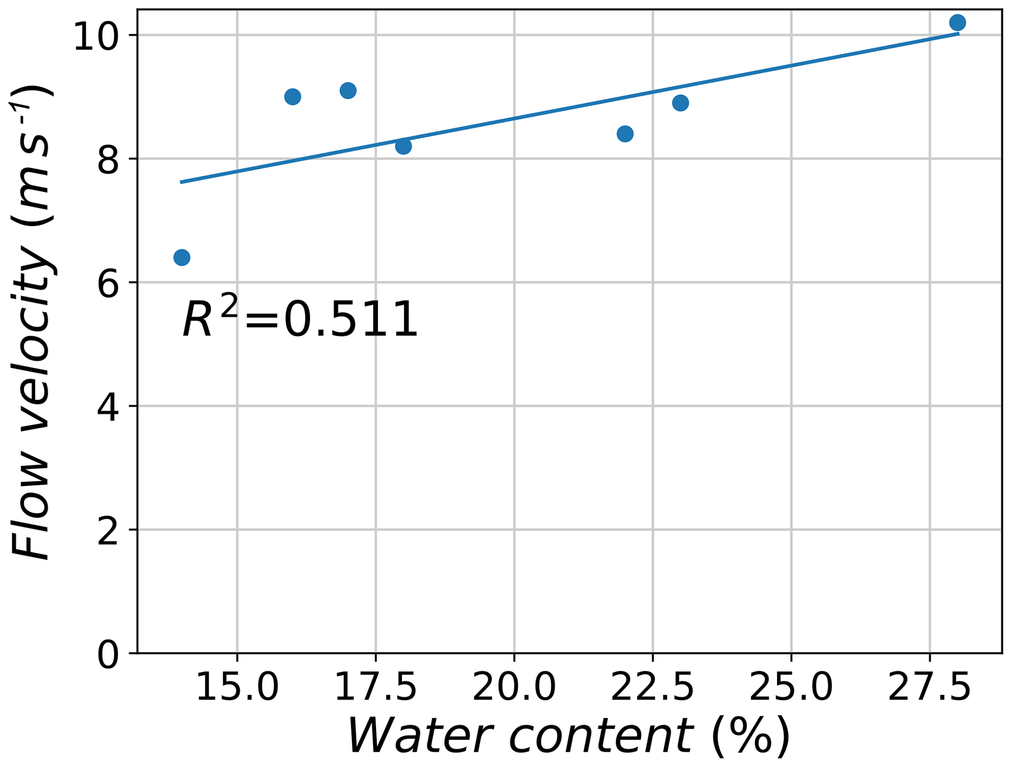
Figure 6Relation between the water content of the granular material of selected experimental tests and the observed mean front velocity.
Another observation can be made regarding the relationship between the amount of fine content (silt and clay) in the prepared material in the reservoir and the maximum flow height recorded at position 2, which is found to be inversely proportional (Fig. 7). At low levels of fine content (21 %–28 %), maximum flow heights were found to be between 0.33 and 0.40 m. A high increase in fine content, like in test no. 9, resulted in a drop in measured flow height to 0.29 m. However, such a relationship is not very evidently inverse. This is because for test no. 16, although the fine content was high (41 %), the recorded flow height was found to be larger than the average for all tests (0.37 m).
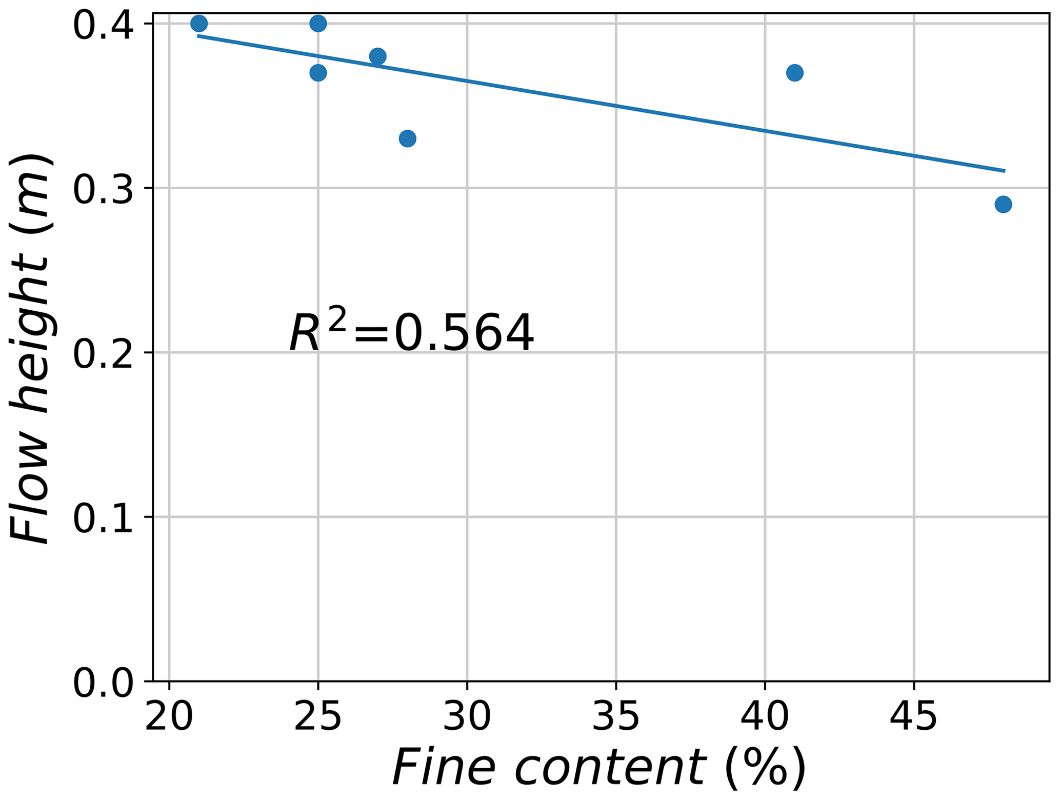
Figure 7Relation between the fine content (silt and clay) of the granular material of selected experimental tests and the observed maximum flow height.
In general, such observations of possible relations between initial flow conditions of the granular material and flowing height and velocity support a calibration process based on those two parameters in addition to the pressure applied to the large sensor. These three parameters were found to vary with each test, but with different percentages. The flowing height was found to have the lowest variations as it ranges between 0.29 and 0.4 m. Its maximum variation was recorded for test no. 9, which has a flow height of 0.29 m, which is 20 % lower than the mean flow height of all tests. Figure 8 shows the variation in mean flow velocity and impact pressure on the larger sensor for the seven selected tests. Similar values of mean front velocity between sections 1 and 2 were observed for tests 10 to 15, while tests 9 and 16 showed higher variations around the mean value. For example, the velocity value of test no. 16 was 6.4 m s−1, which is 22 % lower than the mean of all tests. The highest variation is present in the pressure values, which varied between 15 % and 42 % below and above the mean for tests 9 and 14, respectively.
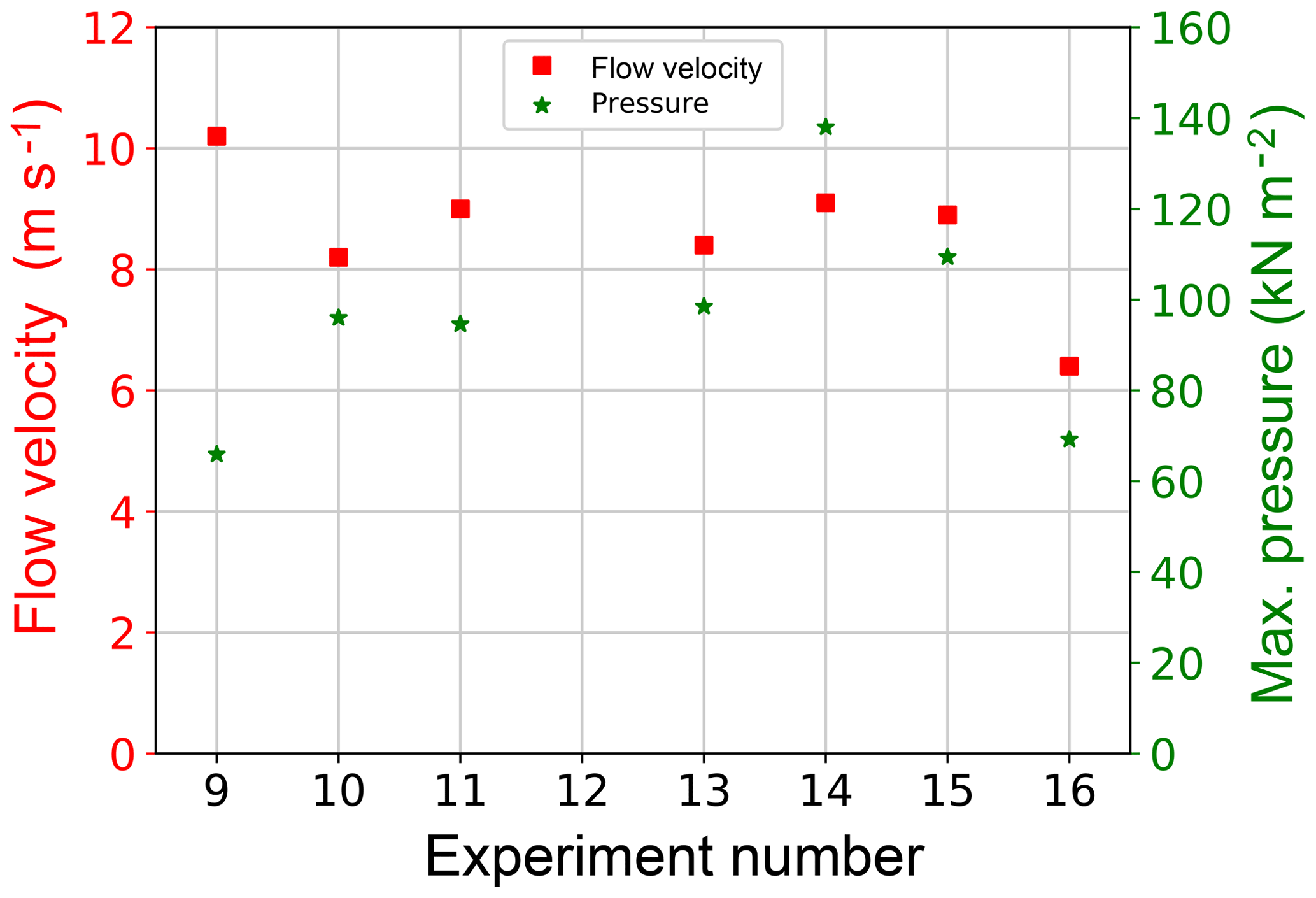
Figure 8Measured mean flow velocity and maximum impact pressure for different experimental tests.
3.2 Results of sensitivity analysis
In this section, the effect of filtering interval of the pressure signal for different simulation results is investigated in detail in order to choose the optimal value of that interval. Afterwards, a detailed parametric study is carried out for the set of parameters of the simulation which was found to agree the most with the different experimental tests (i.e., simulation with ϕb=30∘ and ). The effects of variation in ϕb, , kc, d50 and the chute inclination angle (α) are introduced. The observed effects on the measured flow height, flow velocity and applied pressure are then discussed. For convenience, height, velocity and pressure results of the different sensitivity analysis tests are normalized by values of the baseline simulation with ϕb=30∘ and .
3.2.1 Filtering interval of pressure data
In the full-scale experiments of Bugnion et al. (2012), a filtering interval of 0.05 s was applied to the pressure signal in order to smooth sensor plate vibrations resulting from the impact of solid grains. This technique was found efficient in smoothing peaks and thus calculating representative maximum pressure values of the impacting flowing material. On the other hand, for discrete element simulations, a similar challenge is present due to the discrete nature of the impact between flowing particles and the sensor wall, although no vibration of the sensor takes place. Raw DEM signals usually have strong oscillations and thus it is important to apply a filtering interval to those signals (Chanut et al., 2010; Albaba et al., 2015; Kneib et al., 2017, 2019). The use of the same filtering signal as that of the experiment would be irrelevant since the source of oscillation is different. The strong oscillations of DEM signals are usually linked to many factors including the number of particles, the area that is being impacted, the frequency of recording data, the mean particle diameter and the number of contacts. Furthermore, particles in the DEM simulations range between 50 and 100 mm in size for a typical simulation, which represents only a fraction of the real grain size distribution of the experiments (less than 30 % in mass). Moreover, the model is calibrated against experiments of full-scale hillslope debris flow with a volume of 50 m3. Such a large volume requires running the simulation with particle sizes that are relatively large (d50=75 mm) in comparison with the particle size distribution of the experiment, in order to keep the total number of particles within computationally feasible limits (i.e., the average total number of particles is around 160 000). In addition, the pressure-measuring sensor of the experiment is small in size (200 mm × 200 mm) in comparison to the mean particle size considered for the simulations (75 mm), which results in a fewer number of contacts per impact.
Moreover, the possible variation in the particles' initial spatial distribution in the released material might also have an effect on the force signal, as reported in some DEM studies (e.g., Albaba et al., 2015). Because of all aforementioned reasons, there was a need to define a filtering interval based solely on an investigation of the DEM signal and independent of the experiment's filtering interval. First, the same DEM simulations (using ϕb=30∘ and ) were carried out 10 times with different initial spatial distributions and then the maximum pressure was analyzed using different filtering intervals (0.025 s up to 0.25 s). The same analysis was carried out for the different simulations with different combinations of ϕb and . An optimum filtering interval was identified as that with a relative error lower than 5 %. The relative error is defined as the normalized difference between two successive values of maximum impact pressure for each simulation. After analyzing all simulations and testing different filtering intervals, a filtering interval of 0.15 s was found to be adequate for producing relative errors lower than 5 % for all simulations and thus has been selected for representing pressure values of the simulations. Figure 9 shows the variation in the maximum impact pressure and relative error for different filtering intervals for four simulations. A simulation labeled “2033” indicates a simulation with ϕb=20∘ and a ratio of .
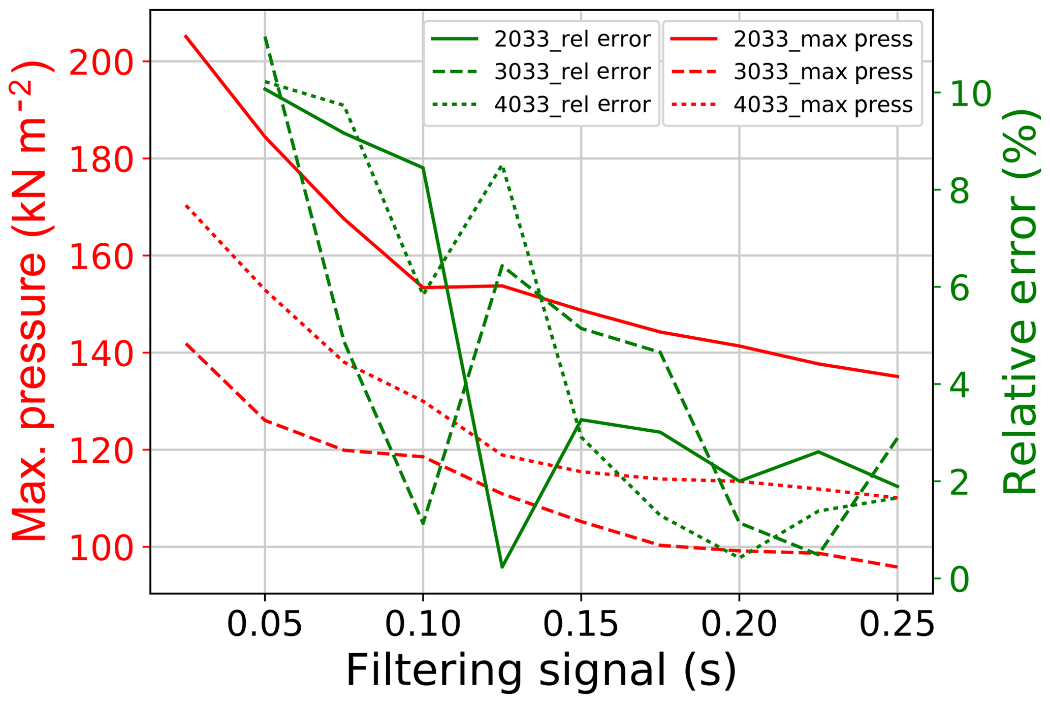
Figure 9Maximum impact pressure and its corresponding relative error for different values of the filtering interval. Results for 2033 indicates a simulation with ϕb=20∘ and .
3.2.2 Basal friction coefficient
The microscale basal friction angle (ϕb) between flowing particles and the chute base is varied from 20 to 40∘ with a 5∘ increment. Figure 10 shows the effect of this variation on measured parameters in the simulations. Flow height is found to increase when increasing the basal friction. Simulations with ϕb=20∘ record maximum flow heights that are 20 % lower than those with ϕb=30∘, while that of ϕb=40∘ is 24 % larger. This could be due to the increase in the basal resistance to flow shearing, which increases the number of particles in the vertical direction perpendicular to chute base. An inverse relation is observed for the flow velocity, which is found to decrease by increasing the basal friction. This is due to the increase in the resistance to movement by the chute base. This decrease in flowing velocity has a direct impact on the value of maximum impact pressure, which is found to decrease with increasing basal friction. A sharp decrease is observed for pressure values when decreasing basal friction angle from 20 to 30∘. Further decrease is however found to have a limited effect on the recorded pressure values. Overall, the observed relationship between flowing velocity and impact pressure is governed by the increase in kinetic energy of the flowing mass (Faug et al., 2009; Jiang and Towhata, 2013; Albaba et al., 2018).
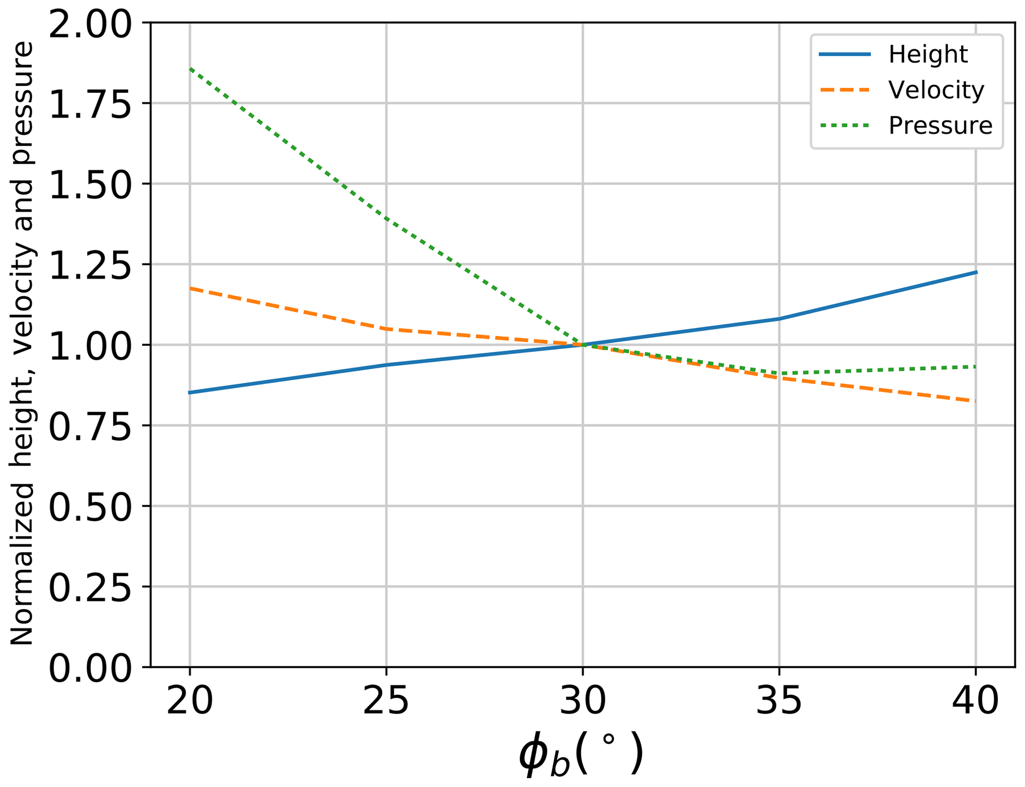
Figure 10Variation in flow height, velocity and pressure for different values of basal friction angle (ϕb) when normalized by results of the simulation with ϕb=30∘, , d50=75 mm and α=30∘.
3.2.3 Ratio between stiffness parameters ()
Figure 11 shows the effect of varying the ratio between stiffness parameters () on the flow height, the velocity and the pressure. Six values of are tested: 0.30, 0.33, 0.36, 0.39, 0.42 and 0.45. Modifying the value of results in a change in k2 since k1 is fixed. For the flowing height and velocity, a small gradual increase is observed in their values with the increase in . This might be due to the decrease in plastic deformation at the microscale, which leads to more dispersion of particles away from the center of the flowing mass. On the contrary, for the impact pressure, an increase in results in a considerable decrease in the value of maximum impact pressure. The difference is very small for an increase in from 0.3 to 0.33. However, further increase in results in a systematic decrease in the maximum applied pressure, which reaches a 40 % decrease for in comparison to . This decrease could be due to a large dispersion of particles leading to a more gradual impact on the sensor.
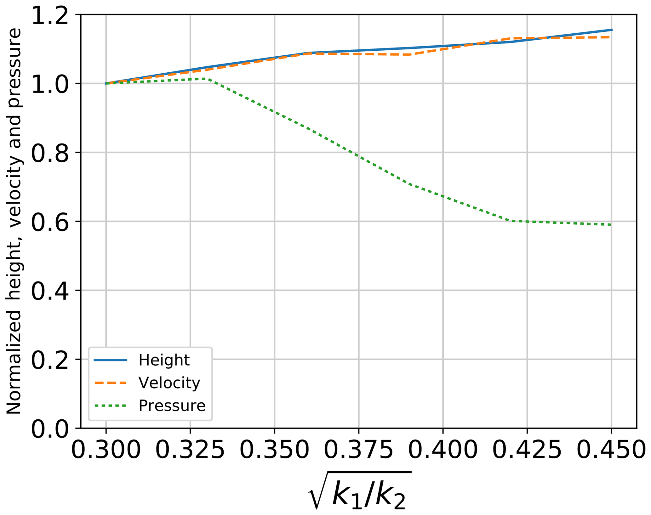
Figure 11Variation in flow height, velocity and pressure for different values of the ratio between stiffness parameters () when normalized by results of the simulation with ϕb=30∘, , d50=75 mm and α=30∘.
3.2.4 Adhesive stiffness parameter (kc)
Figure 12 shows the effect of varying the adhesive stiffness parameter (kc) on the flow height, the velocity and the pressure. Four values of kc∕k1 are tested: 0.5, 1.0, 1.50 and 2.0. Modifying the value of kc∕k1 results in a change in kc since k1 is fixed. The observed changes in the maximum flowing height at position 2 as well as the mean front velocity between positions 1 and 2 are negligible. A slight change in the pressure applied to the large sensor is observed when increasing kc, especially when kc is larger than k1. The recorded impact pressure is found to increase 20 % when doubling the value of (kc).
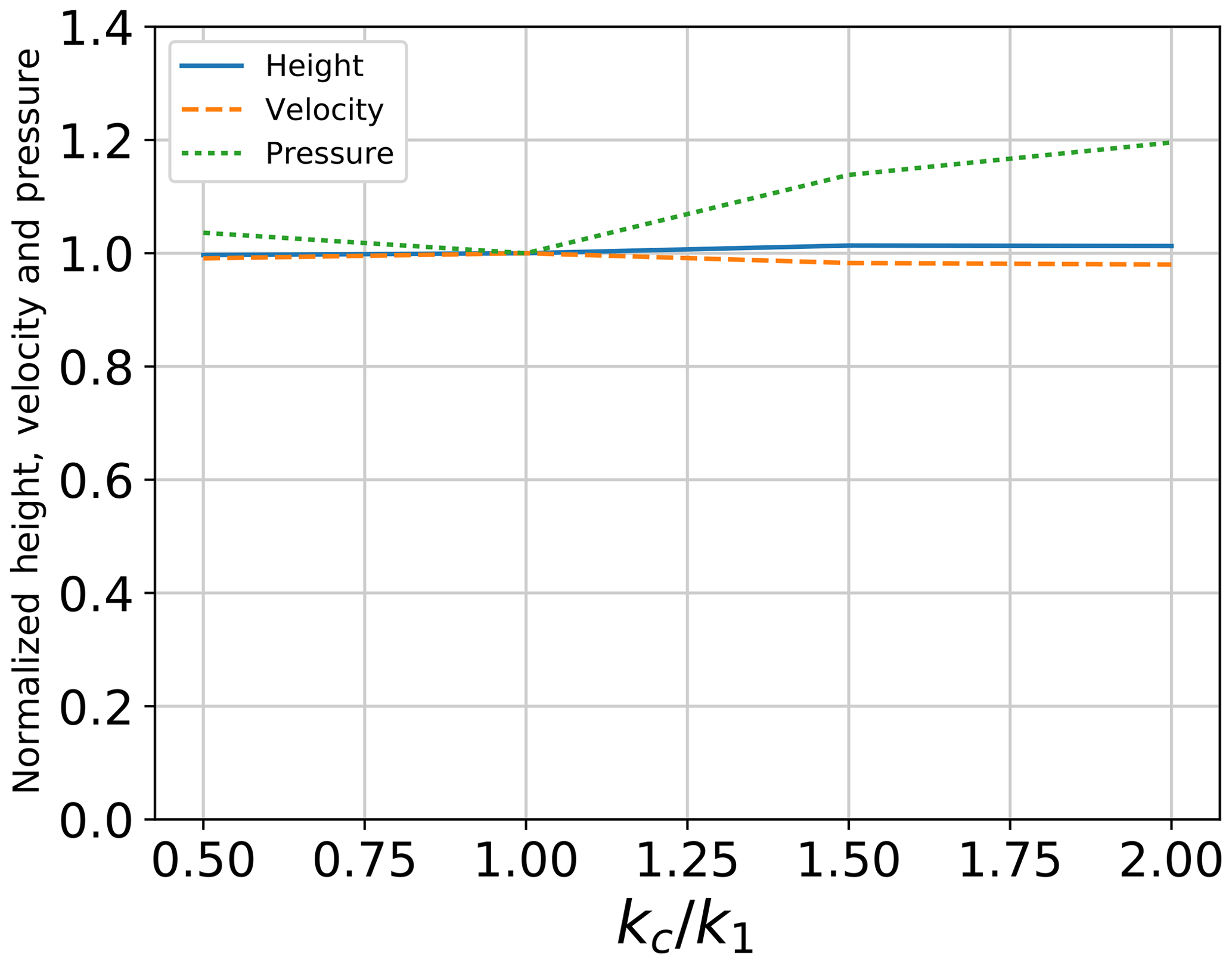
Figure 12Variation in flow height, velocity and pressure for different values of the adhesive stiffness parameter (kc) when normalized by results of the simulation with ϕb=30∘, , d50=75 mm and α=30∘.
3.2.5 Mean particle diameter
Four samples with different values of d50 are tested: 75, 100, 125 and 150 mm. Values of the normalized maximum flow height at position 2, mean front velocity and maximum applied pressure on the large plate are shown in Fig. 13. The maximum flow height at position 2 is found to increase when moving from d50=75 to 100 mm while a smaller increase is observed for further increase in mean diameter (simulations with d50=125 and 150 mm). This increase is due to the presence of larger particles in the virtual box where flow height is measured in the model perpendicular to the base of the chute. However, all in all, the observed difference in flow height for the different mean diameters is rather limited and is found not to exceed 25 %, although the mean diameter is doubled. Regarding the flow velocity, negligible changes are observed when varying the mean diameter. Flows in the different simulations are found to arrive at similar times at position 2, thus having similar mean front velocities. Concerning the impact pressure on the large plate, a considerable difference is observed when comparing the different particle sizes. The maximum pressure for simulation with d50=150 mm is 1.8 times larger than that of d50=75 mm. In addition, the pressure is found to increase with the increase in mean diameter, except for d50=100 and 125 mm. For those two tests, normalized pressure values are 1.66 and 1.50, respectively. Further discussion of the effect of mean particle diameter on the observed flow height, velocity and impact pressure is presented in the discussion section.

Figure 13Variation in flow height, velocity and pressure for different values of mean particle diameter (d50) when normalized by results of the simulation with ϕb=30∘, , d50=75 mm and α=30∘.
3.2.6 Inclination angle
To investigate the effect of changing the chute inclination angle (α), which was fixed at 30∘ for all other simulations in accordance with the test site in Veltheim, four additional values of α are tested: 20, 40, 50 and 60∘. It was noted during the simulations that an inclination angle of 20∘ did not reproduce a dense flow but a very discrete flow of particles instead. This is because the value of basal friction ϕb is larger than α (GDR-MiDi, 2004). As a result, the simulation case with ϕb=20∘ will be ignored in the results analysis.
The change in inclination angle has an effect on the maximum flow height at position 2 (Fig. 10), which increases with 20 % for a change in α from 30 to 60∘. A larger effect is observed for the mean front velocity, which increases by 100 % for an increase in α to 60∘. Such an increase has a direct link to the maximum applied pressure, which increases by 465 %.
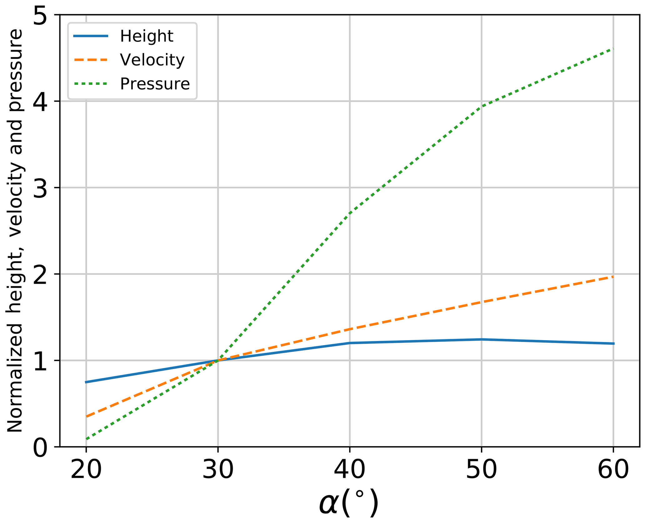
Figure 14Variation in flow height, velocity and pressure for different values of inclination angle (α) when normalized by results of the simulation with ϕb=30∘, , d50=75 mm and α=30∘.
All in all, the sensitivity analysis of the model's parameters showed the highest sensitivity of the flow height, velocity and pressure to the variation in basal friction angle and the ratio between stiffness parameters. In the next section, different simulations with varying values of ϕb and are compared to the experimental data in terms of flow height, velocity and pressure in order to find the best-fit parameter combination for each experimental test.
3.3 Cross comparison between DEM simulations and field experiments
3.3.1 Flow height and velocity
Figure 15 shows the comparison between the measured maximum flow height at section 2 in the selected field experiments with values of their corresponding best-fit numerical simulations. It can be seen that a very good agreement is observed for tests 10 and 11 when compared with the DEM results. For tests 13–16, a relatively good agreement is observed with the maximum margin of error being 15 %. The least agreement is shown for test no. 9, which has an error of almost +38 %. This test showed the highest variation from the mean when compared with other experimental tests.
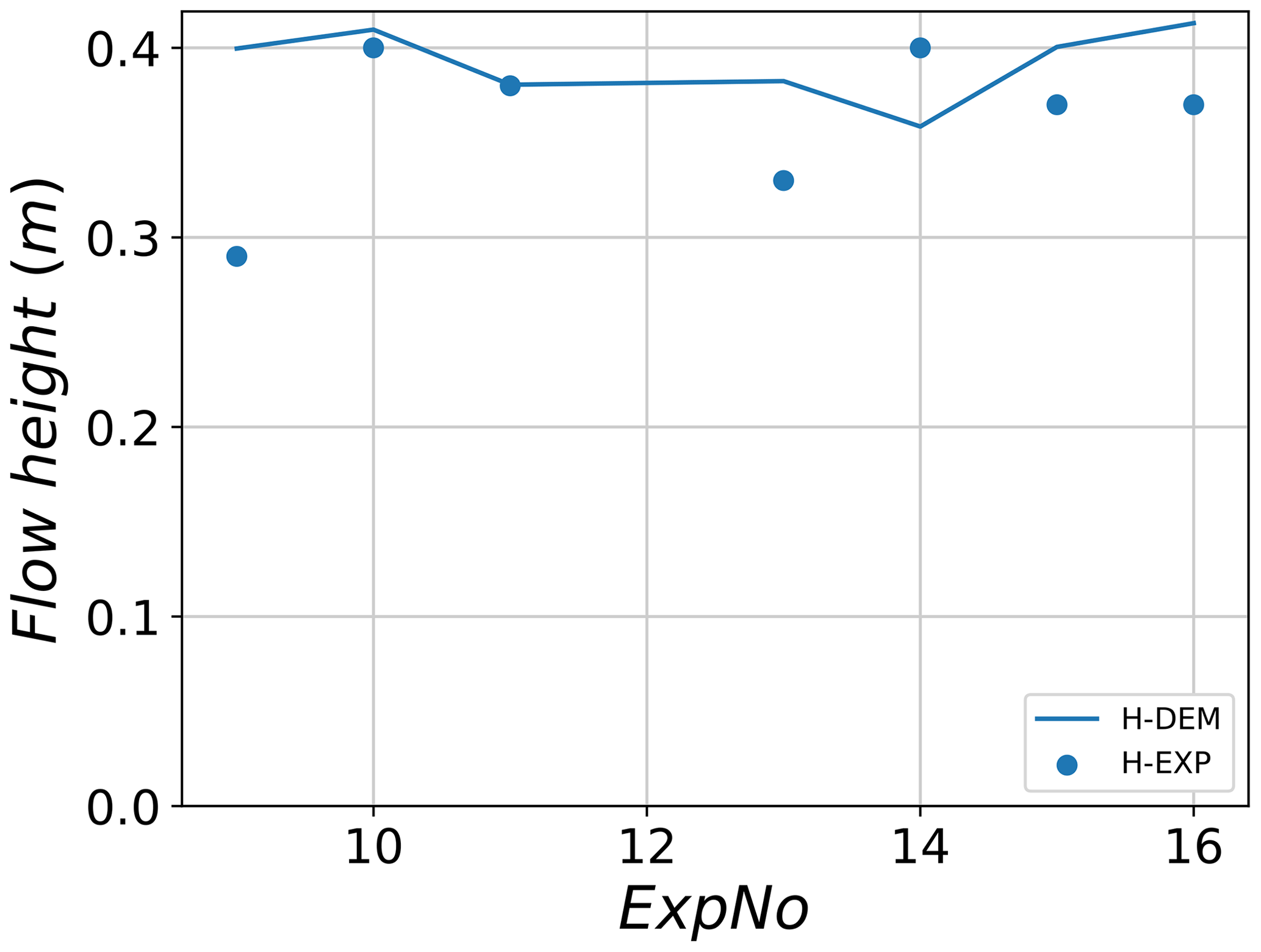
Figure 15Maximum flow height at section 2 for experimental data (H-Exp) and their corresponding best-fit DEM simulations (H-DEM).
For flowing velocity, a better general agreement between the experiment and DEM results is observed (Fig. 16). For example, for tests 10, 11 and 13, the observed mean velocity is well reproduced by the DEM. For tests 14 and 15, a relatively similar flow velocity of 8–9 m s−1 is observed for both the experiment and the model. The only strong disagreement between the model and experiment is observed for test no. 16 for the which the experimental value is 6.4 m s−1 and the corresponding best-fit simulation flow velocity is 8.5 m s−1.

Figure 16Flow front velocity, measured between sections 1 and 2, for experimental data and their corresponding best-fit DEM simulations.
3.3.2 Impact pressure
Figure 17 shows the maximum impact pressure applied to the large sensor for both the experiment and DEM simulations. Very good agreement is observed for most experiments when compared with their corresponding best-fit simulations. For test no. 9, the maximum pressure recorded during the experiment was equal to 65.9 kPa while the corresponding best-fit value recorded in the simulation was 73.8 kPa, resulting in an error of +11 %. All other tests had lower values of error when comparing pressures between the experiments and best-fit simulations. The best agreement is observed for tests 11, 15 and 16 where the errors do not exceed 4 %.

Figure 17Maximum pressure applied to the large sensor for experimental data and their corresponding best-fit DEM simulations.
It is however important to compare the pressure evolution for the different tests, in addition to the comparison with peak pressure values. This is because the same peak pressure value could be achieved with different pressure evolution. A higher filtering interval has been applied to pressure signals of both the experiment and the DEM simulations in order to obtain pressure evolution curves that can be compared properly.
The evolution of pressure applied to the large sensor during the experimental test no. 9 is shown in Fig. 18 along with its corresponding best-fit DEM simulation. At the beginning of the impact ( s), the DEM curve starts recording pressure values which are due to the dilute group of particles that are detached from the main flow and individually impact the rigid wall representing the pressure sensor in the simulation. Afterwards, the two curves agree well with each other until reaching similar peak values at similar time points (64 and 70 kPa for the experiment and DEM, respectively). After the phase of maximum impact pressure, both pressures start decreasing with similar rates until t=6.35 s. A further decrease in pressure is found to be faster in the experiment in comparison with the DEM where the decrease occurs over longer periods of time. At the end, the pressure signal in DEM is found to lag 2 s behind that of the experiment.
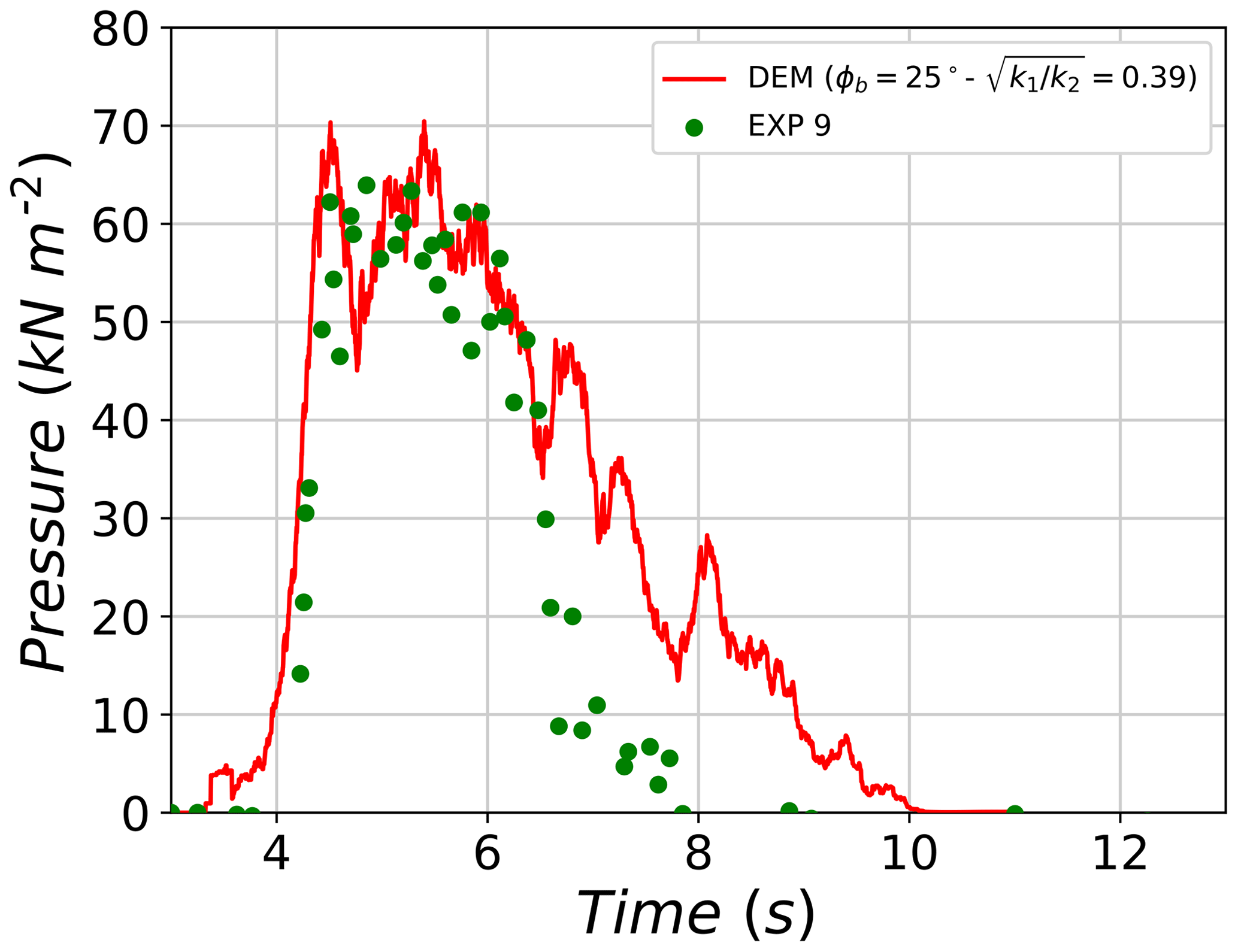
Figure 18Evolution of the impact pressure on the large plate for test no. 9 and its respective DEM best-fit simulation.
Similar observations can be made when comparing pressure values of test no. 14 with its corresponding DEM simulation (Fig. 19). A first phase of impact of the dilute group of particles causes pressure values to increase for the DEM with no equivalent increase in the experiment. Afterwards, both pressure curves agree well until reaching very similar peaks (122 and 128 kPa for the experiment and DEM, respectively). The decrease in pressure that follows the reached peaks has similar rates for both the experiment and DEM until t=8 s. Afterwards, pressure values of the experiment decrease faster while those of DEM lag behind, causing the total impact duration of the DEM to be larger than that of the experiment.
Tests 11, 13 and 15, which had very similar initial conditions of the granular material and also similar values of measured parameters (height velocity and pressure), were found to be best fitted with similar parameter sets in YADE (ϕb=(25, 30, 30∘), , 0.30, 0.33)). For example, the comparison of pressure values recorded during experiment no. 15 and its corresponding DEM best-fit simulation reveals a similar trend (Fig. 20). At the beginning, the evolution of pressure signal in the DEM starts slightly earlier than that of the experiment. Afterwards, a sharp increase in pressure is observed for the experiment and DEM, where both reach peak impact force values in a very short period of time. The reached peaks are very similar in value and correspond to 100 kPa for both signals. Next, after the peak, pressures values of the experiment decrease at a similar rate as that of DEM until t=6.5 s. A further decrease in pressure signal is faster for the experiment, while the DEM signal is delayed but with a smaller margin when compared to previous differences between the experiments and the DEM simulations.
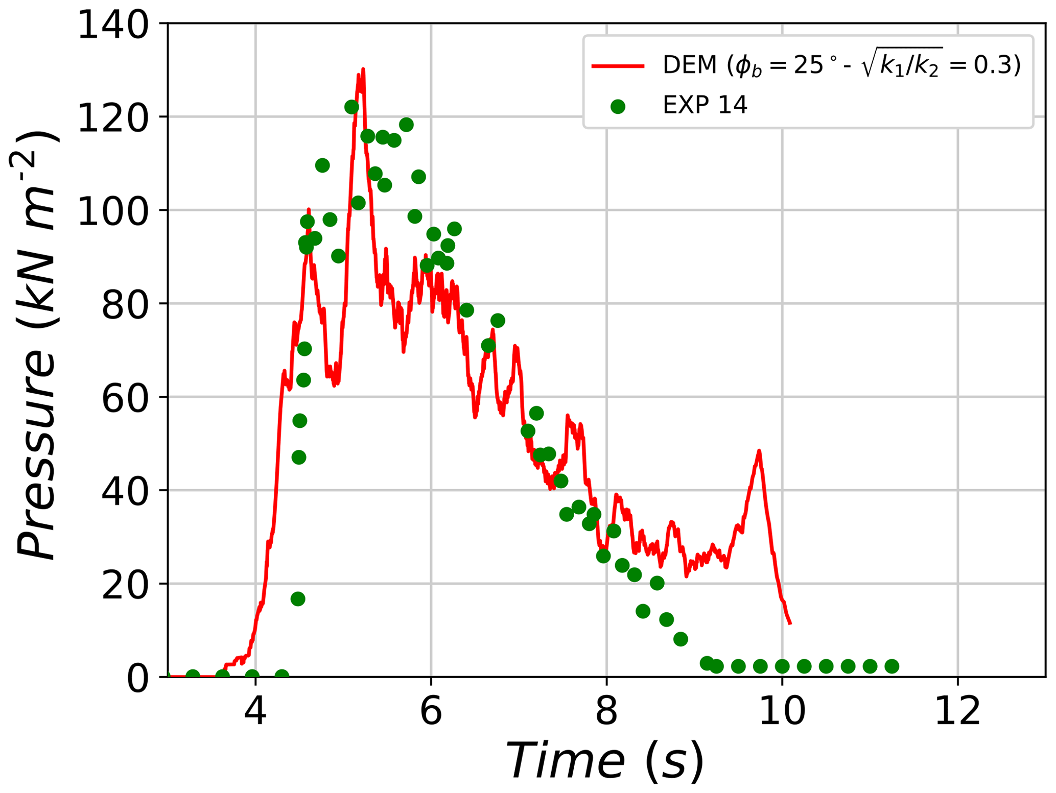
Figure 19Evolution of pressure on the large plate for test no. 14 and its respective DEM best-fit simulation.
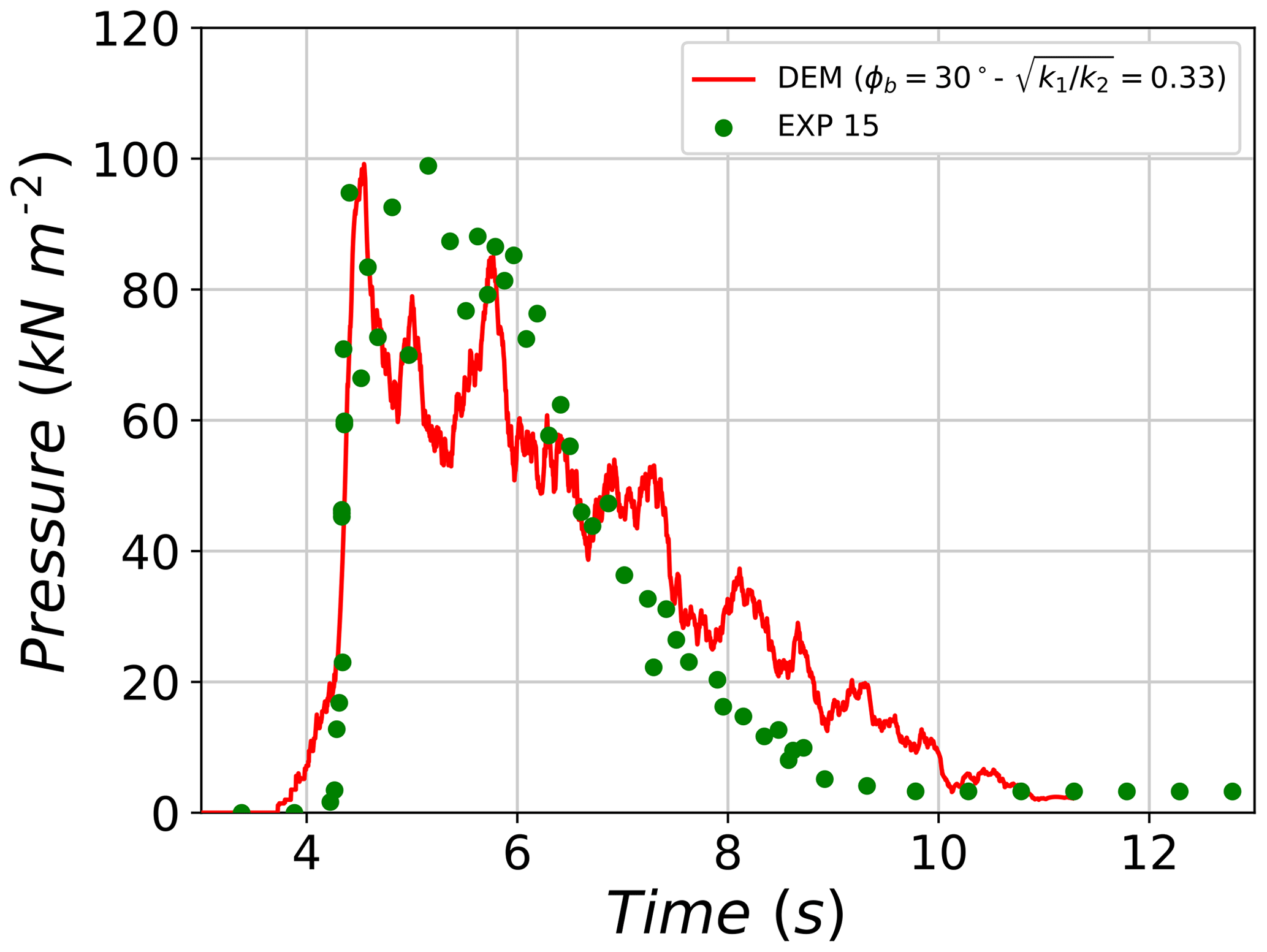
Figure 20Evolution of pressure on the large plate for test no. 15 and its respective DEM best-fit simulation.
The last comparison concerns test no. 16, which is found to agree well with its corresponding best-fit DEM simulation concerning pressure evolution. Apart from the early start of the DEM curve (around 0.5 s earlier), which is due to the dilute front, both curves are found to reach very similar peak pressure values (65 kPa for the experiment and 69 kPa for the DEM simulation) at a similar time point (t=5.2 s). Then both pressure curves start decreasing with similar rates until t=7.5 s. Pressure values of test no. 16 are then found to decrease faster than those of the simulation until reaching static pressure values of around 12 kPa, which indicates the deposit of some material on the pressure sensor. The DEM curve progressively decreases over a longer period of time until decaying to zero at t=12.1 s.
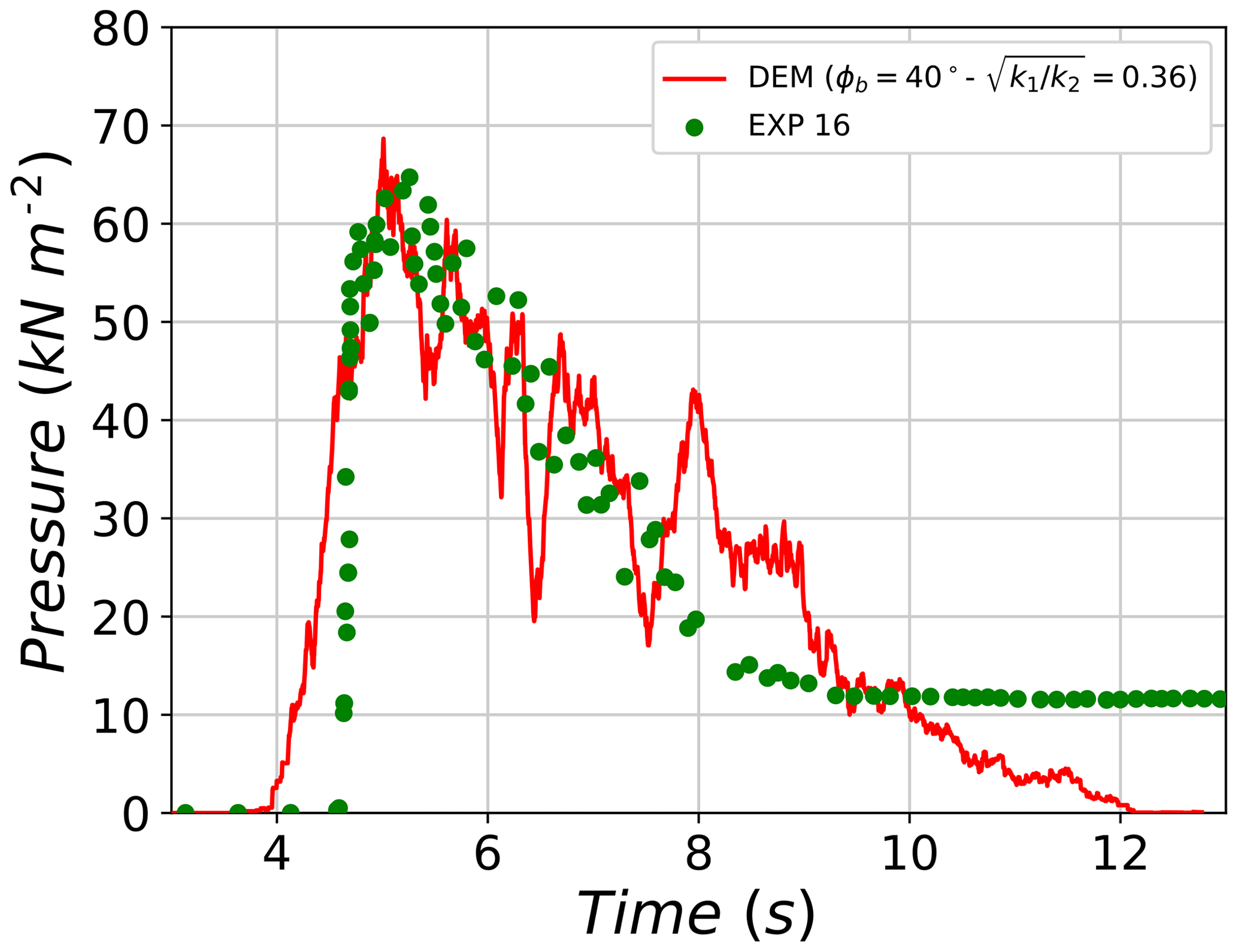
Figure 21Evolution of pressure on the large plate for test no. 16 and its respective DEM best-fit simulation.
3.3.3 Best fit
Results of all DEM simulations are best fitted against experimental data of tests at the Veltheim site using Eq. (5). Figure 22 shows the correspondence between experimental tests and their respective best-fit DEM parameters, based on comparisons of flow height, flow velocity and impact pressure on the large sensor. Tests 10, 11, 13, 14 and 15 are found to be reproducible with very similar values of the parameter set and ϕb (Fig. 22). Those tests are found to have similar values of water content in the granular material prepared in the reservoir (between 16 % and 23 %). In addition, they tend to have similar values of fine content (silt and clay), which ranges between 21 % and 28 %. Test no. 9 is best reproduced by and ϕb=25∘ while test no. 16 is best reproduced by and ϕb=40∘. Further analysis of the best-fit results and possible relations between model parameters and granular samples' initial conditions are discussed in Sect. 4.2.
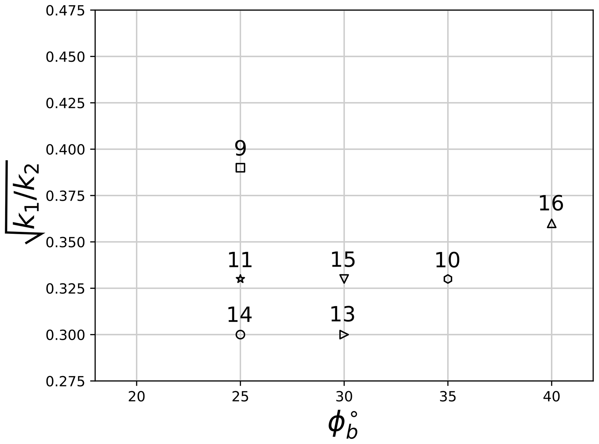
Figure 22The best-fitting set of parameters ( and ϕb) for each of the selected experimental tests based on comparison of flow height, mean front velocity and maximum applied pressure.
4.1 Phenomenology of impacting pressure
Results of the field experiments showed that the highest varying parameter was the maximum impact pressure (Fig. 8). These high variations in pressure were possibly due to the interaction between large boulders of the flow and measuring senors in short periods of time, although this effect was minimized by filtering the data over a period of 0.05 s. This phenomenon is supported by the fact that although some tests had similar initial conditions (water and fine content) and also similar flowing height and velocity, the maximum recorded pressure was largely different. This is clear when comparing tests no. 11 and 14, which had similar values of initial and flowing conditions but different pressures of 94.6 and 138 kPa, respectively.
Comparisons of pressure evolution of the selected experimental tests and the DEM simulations revealed general agreement in peak pressure values and impacting trend. However, some discrepancies were observed concerning impact rate and duration. The nature of DEM simulations, in which a group of particles interact at the microscale, might have contributed to these observed differences. For example, pressure signals during DEM simulations were found to start earlier than those of the experimental tests. This was due to the detachment of a group of particles from the mean part of the flow, causing particles to form a dilute frontal part which impacts the pressure sensor early (Fig. 5b). Furthermore, the decreasing phase of the pressure signal was found to last longer for DEM simulations in comparison with experimental tests. The formation of a dilute tail could be responsible for that as it needed a longer time to fully interact with the sensor (a compression phase of the dilute part needs to first occur).
Another important factor governing the impact pressure was found to be the average particle diameter (d50). Since the total released volume is fixed, the number of particles in each simulation decreases with increasing particle size. Figure 23 shows the time evolution of pressure signal for the different tested particle size diameters. Pressure signals are found to start at relatively the same time, indicating a similar flow arrival time to impact the sensor. Afterwards, the peak impact pressure is reached at different time points for the different diameter sizes. Simulations with smaller particle sizes reach the peak earlier than those of larger particle sizes. However, this observation might depend on the possibility of a larger particle impacting the sensor at a specific time step. More significant is the rapid increase and decrease in the pressure signal, which is found to increase by increasing the diameter size. This could be attributed to the force chain distribution behind the wall. Force chains are strongly dependent on the particles' position and orientation with respect to the object they impact (Azéma and Radjaï, 2012), which in this case is the large sensor. The distribution of contact forces on the sensor is expected to be different from one simulation to another, depending on the number of contacts and the position of large and small particles behind the sensor (Albaba et al., 2015). Figure 24 shows the maximum impact pressure and average number of contacts for different particle sizes. The use of d50=0.075 m results in an average number of contacts for the full period of impact of 3.6. This number of contacts decreases rapidly with increasing average particle size reaching 1.8 contacts for d50=0.10 m and 1.4 contacts for d50=0.15 m. Furthermore, the maximum impact pressure is found to be inversely related to the number of contacts with the sensor.
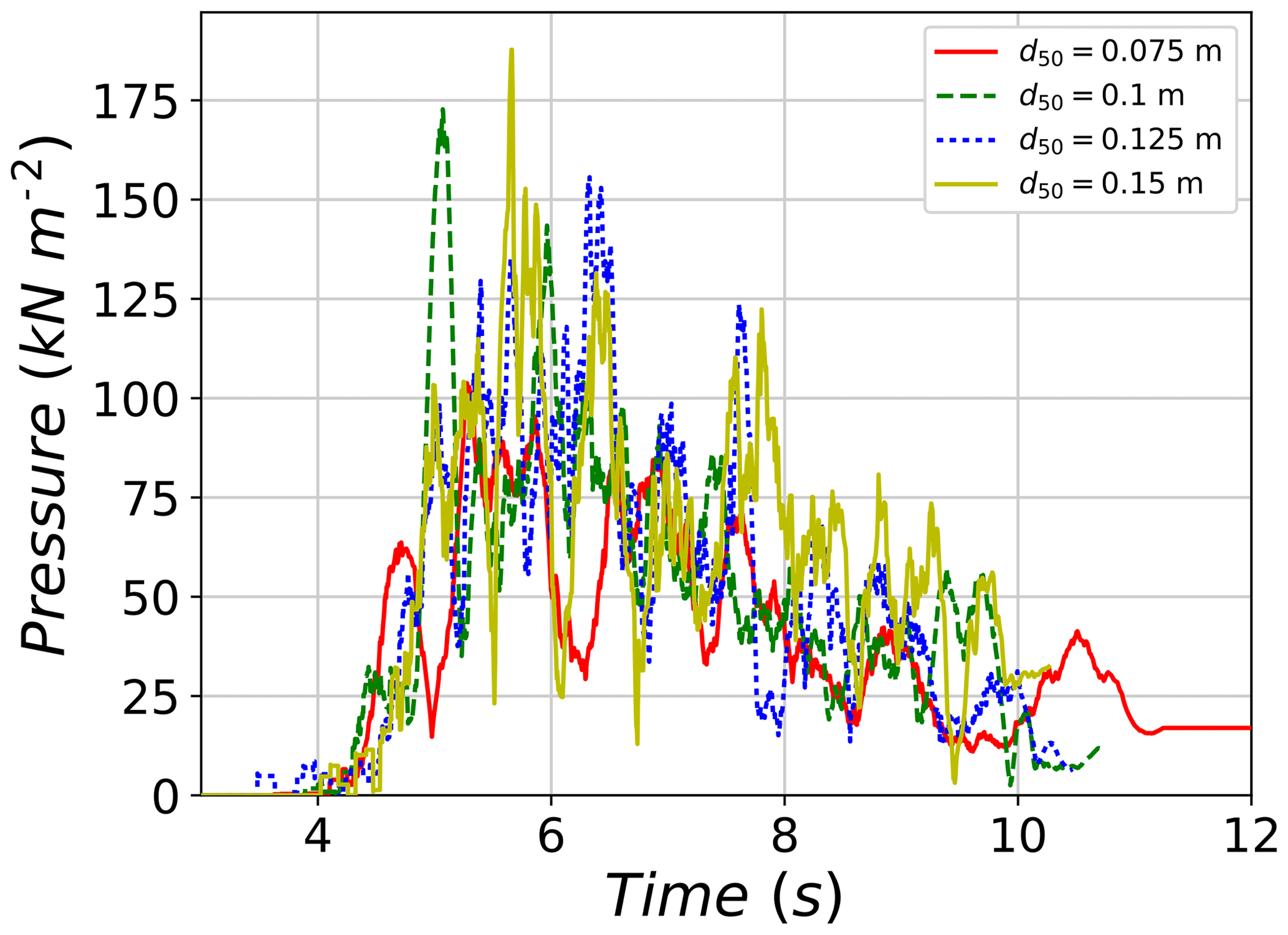
Figure 23Evolution of pressure on the large plate for different simulations with different d50, using ϕb=30∘, and α=30∘.

Figure 24Maximum impact pressure and average number of contacts for different simulations with different d50, using ϕb=30∘, and α=30∘.
These observations support the assumption that pressure values are mostly dominated by hard contacts with large solid grains. Such contacts influence the pressure signal, although their influence is reduced by the application of filtering windows. The probability of a large particle impacting the pressure sensor increases by increasing the mean diameter because of the decrease in the number of contacts. As particles grow in size and reduce in number, impact mechanisms tend to be similar to those of rockfalls (points loads) rather than those of debris flows (gradual cross-sectionally spread loads). The decrease in maximum pressure of the test with d50=125 mm in comparison with that of d50=100 mm can be understood through the random positioning of particles that are created in the box of the initial released volume. Particles are created with random position at each simulation, which leads to different distributions of particles in the flowing and impacting phases.
4.2 Best-fit parameter set
Results of best-fit simulations based on flow height, mean front velocity and maximum applied pressure revealed that experimental tests (11, 13 and 15) could be reproduced using similar parameter sets in the DEM, as already seen in Sect. 3.3.3. Test nos. 9 and 16 were found to be reproduced with a very different parameter set. The difference in numerical best-fit parameters can not be explained by the pressure values, which are very similar for both tests (65.9 and 69.2 KPa for tests 9 and 16, respectively). Despite this fact, test no. 9 recorded the highest-mean front velocity (10.2 m s−1), possibly due to having the highest water content (28 %). Unlike other tests, such high-speed flowing material did not contribute to a high pressure value mainly because this test had the highest amount of fine material (i.e., lowest percentage of sand) and consequently the lowest wet density (1790 kg m−3). All these conditions are reflected in the value of best-fit basal friction angle parameter in the DEM simulation, which is among the lowest for all best-fit simulations.
On the other hand, test no. 16 had a low water content in the released material (14 %) but a relatively high fine content (41 %). This contributed significantly to its wet density, making it the highest among all tests (2110 kg m−3). However, the low water content of the granular material might have led to its low mean front velocity, which was the lowest among all tests (6.4 m s−1). This low flowing velocity was probably the main reason for the low maximum pressure value recorded during that test. All these initial conditions (especially the low water content) were reflected in the value of best-fit basal friction angle parameter in the DEM simulation, which is highest among all best-fit simulations (40∘).
It is worth noting that attempts to base the best-fit solely on one part of Eq. (5) did not produce consistent results in terms of the relation between the initial conditions of the experimental test and the model parameter set and ϕb (see Fig. A1 in Appendix A, which shows results of best-fit comparisons based separately on the flow height, the flow velocity or the impact pressure).
All in all, to draw strong conclusions on the relationship between initial conditions of granular samples and YADE model parameters, experimental data with a wider range of both water content and fine content are needed. The experimental data considered here had a narrow range of variation in both of those parameters, which was reflected in the narrow variations in maximum flow height values. Since field experiments are expensive and difficult to organize, lab experiments can be used instead in order to study the effect of those parameters in detail.
Rapid urbanization of mountainous areas has contributed to the focus on studying the different types of mass movement such as landslides and hillslope debris flows. In this study, a discrete-element-based contact law was implemented for the purpose of modeling hillslope debris flow. The model has three phases which are elastic, plastic and adhesive. The model capabilities in reproducing filed-scale hillslope debris flow experiments were tested in detail. A group of seven experimental tests were selected with varying levels of bulk density, water content and fine content. In each experiment, maximum flow height at a defined section, mean front velocity and maximum impact pressure applied to a measuring sensor were measured. A total of 30 numerical simulations were carried out by varying two parameters in the numerical model (basal friction angle ϕb and the ratio between stiffness parameters ). Calibration of the model against experimental data was based on finding the best-fit set of parameters ϕb and of the model that matches each selected experiment concerning flow height, mean front velocity and applied pressure.
We conclude that a very good agreement between the model and experiments was observed concerning mean front velocity and maximum applied pressure, with less agreement of flow height. Detailed comparisons of pressure evolution between different selected experiments and simulations revealed the model's capability of reproducing observed pressure curves, especially during the primary loading phase, leading to maximum pressure. However, since the model did not simulate the deposition of material on the inclined channel, a post-peak unloading phase similar to the experiments could not be reproduced. The analysis of the best-fit between the model and the experiments showed that many experimental tests were best reproduced with similar ϕb and parameter combinations. These experiments were found to share similar medium values of water and fine content. Increasing the basal friction in the model led to simulations matching the experiment with the lowest water content and highest bulk density. On the contrary, a higher value of and relatively low value of ϕb were needed to reproduce the test with the highest water content and the lowest bulk density. All these findings suggest that a link exists between the model parameters and initial conditions of granular samples. Such a link should be further investigated in detail on the basis of additional hillslope debris flow experiments.
The data of different simulations are not stored in a publicly accessible database due to their large size. They are however available from the corresponding author upon request.
Figure A1 shows results of the calibration of the best-fit parameter set in the model based on the flow height, velocity and pressure (Fig. A1a), only on the maximum flow height (Fig. A1b), only on the mean front velocity (Fig. A1c) and only on the maximum applied impact pressure (Fig. A1d).
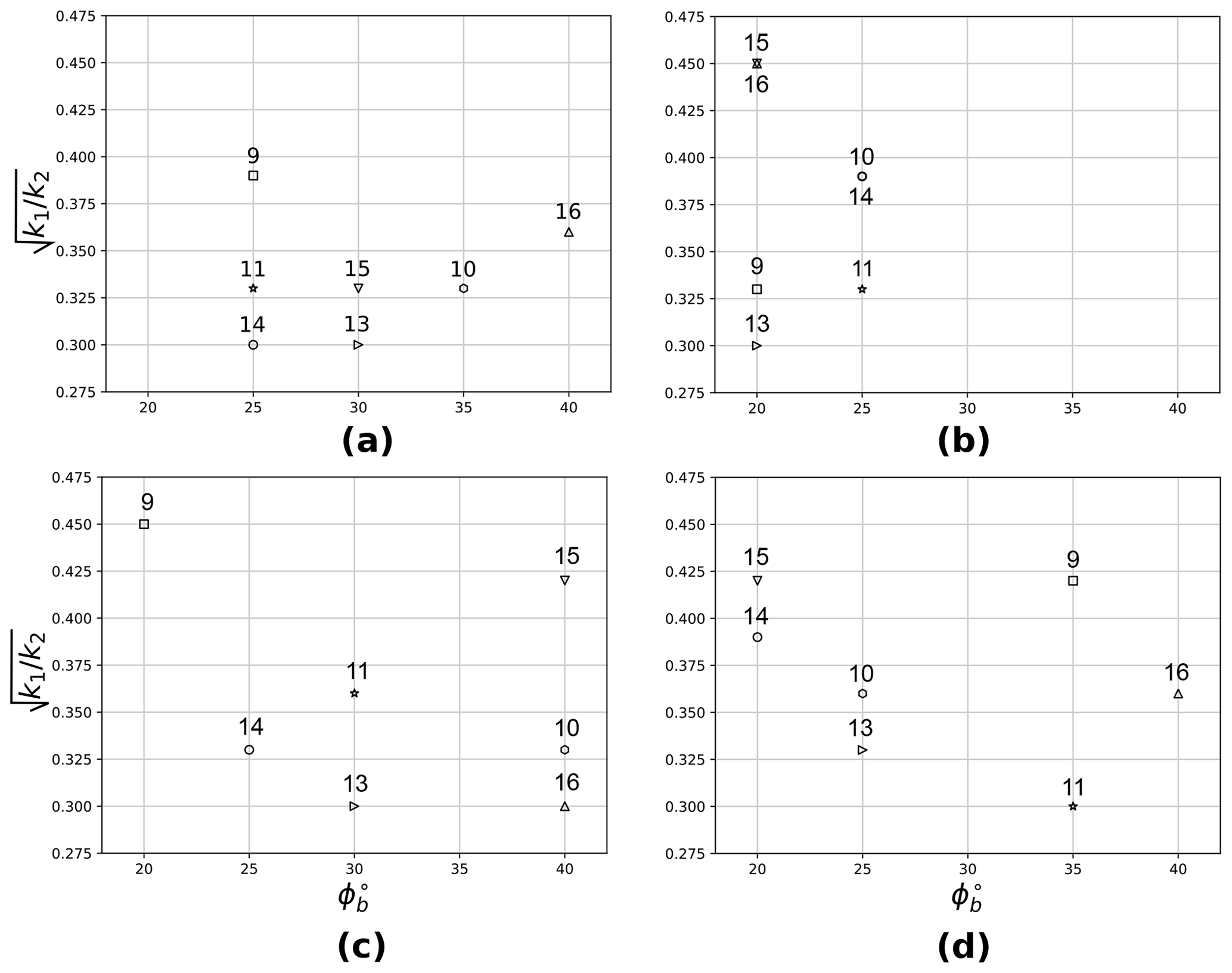
Figure A1The best-fitting set of parameters ( and ϕb) for each of the selected experimental tests based on all three parameters (a), only the flow maximum height (b), only the mean front velocity (c) and only the maximum impact pressure (d).
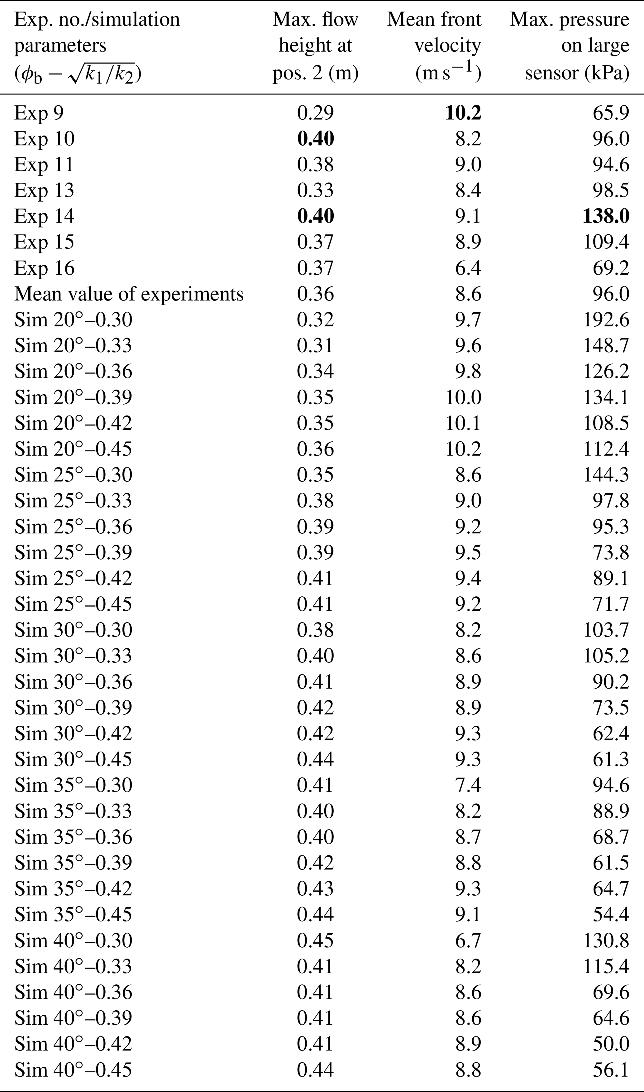
The results concerning the maximum flow height at position 2, the mean front velocity and the maximum impact pressure of all selected experiments and all the simulations we carried out are shown in Table B1.
Table B1Values of the maximum flow height at position 2, the mean front velocity and the maximum applied pressure for all selected experiments and simulations. Bold text shows the maximum values of the height, the velocity and the pressure of all selected experiments.
The order of the authors' names reflects the size of their contribution to the writing of this paper.
The authors declare that they have no conflict of interest.
The authors thank the reviewers Stéphane Lambert and Alessandro Leonardi for their constructive comments and suggestions.
This research has been supported by the Swiss Federal Office for the Environment (FOEN).
This paper was edited by Mario Parise and reviewed by Alessandro Leonardi and Stéphane Lambert.
Albaba, A.: Discrete element modeling of the impact of granular debris flows on rigid and flexible structures, PhD thesis, Université Grenoble Alpes, Grenoble 2015. a
Albaba, A., Lambert, S., Nicot, F., and Chareyre, B.: Relation between microstructure and loading applied by a granular flow to a rigid wall using DEM modeling, Granular Matter, 17, 603–616, https://doi.org/10.1007/s10035-015-0579-8, 2015. a, b, c, d, e, f, g
Albaba, A., Lambert, S., Kneib, F., Chareyre, B., and Nicot, F.: DEM Modeling of a Flexible Barrier Impacted by a Dry Granular Flow, Rock Mech. Rock Eng., 50, 3029–3048, https://doi.org/10.1007/s00603-017-1286-z, 2017. a
Albaba, A., Lambert, S., and Faug, T.: Dry granular avalanche impact force on a rigid wall: Analytic shock solution versus discrete element simulations, Phys. Rev. E, 97, 052903, https://doi.org/10.1103/PhysRevE.97.052903, 2018. a, b
Andres, N. and Badoux, A.: Unwetterschäden in der Schweiz im Jahre 2017, Wasser Energie Luft, 110, 67–74, 2018. a
Azéma, E. and Radjaï, F.: Force chains and contact network topology in sheared packings of elongated particles, Phys. Rev. E, 85, 31303, https://doi.org/10.1103/PhysRevE.85.031303, 2012. a
Brighenti, R., Segalini, A., and Ferrero, A. M.: Debris flow hazard mitigation: A simplified analytical model for the design of flexible barriers, Comput. Geotech., 54, 1–15, https://doi.org/10.1016/j.compgeo.2013.05.010, 2013. a
Bugnion, L., McArdell, B. W., Bartelt, P., and Wendeler, C.: Measurements of hillslope debris flow impact pressure on obstacles, Landslides, 9, 179–187, https://doi.org/10.1007/s10346-011-0294-4, 2012. a, b, c, d, e, f
Catalano, E., Chareyre, B., and Barthélémy, E.: Pore-scale modeling of fluid-particles interaction and emerging poromechanical effects, Int. J. Numer. Anal. Meth. Geomech., 38, 51–71, https://doi.org/10.1002/nag.2198, 2014. a
Chanut, B., Faug, T., and Naaim, M.: Time-varying force from dense granular avalanches on a wall, Phys. Rev. E, 82, 41302, https://doi.org/10.1103/PhysRevE.82.041302, 2010. a, b
Christen, M., Kowalski, J., and Bartelt, P.: RAMMS: Numerical simulation of dense snow avalanches in three-dimensional terrain, Cold Reg. Sci. Technol., 63, 1–14, https://doi.org/10.1016/j.coldregions.2010.04.005, 2010. a
Cundall, P. A. and Strack, O. D. L.: A discrete numerical model for granular assemblies, Géotechnique, 29, 47–65, https://doi.org/10.1680/geot.1979.29.1.47, 1979. a
Ding, W.-T. and Xu, W.-J.: Study on the multiphase fluid-solid interaction in granular materials based on an LBM-DEM coupled method, Powder Technol., 335, 301–314, https://doi.org/10.1016/J.POWTEC.2018.05.006, 2018. a
Faug, T.: Depth-averaged analytic solutions for free-surface granular flows impacting rigid walls down inclines, Phys. Rev. E, 92, 62310, https://doi.org/10.1103/PhysRevE.92.062310, 2015. a
Faug, T., Beguin, R., and Chanut, B.: Mean steady granular force on a wall overflowed by free-surface gravity-driven dense flows, Phys. Rev. E, 80, 021305, https://doi.org/10.1103/PhysRevE.80.021305, 2009. a
Gabet, E. J. and Mudd, S. M.: The mobilization of debris flows from shallow landslides, Geomorphology, 74, 207–218, https://doi.org/10.1016/j.geomorph.2005.08.013, 2006. a
GDR-MiDi: On dense granular flows, Eur. Phys. J., 14, 341–365, 2004. a
Graf, C. and McArdell, B. W.: Debris-flow monitoring and debris-flow runout modelling before and after construction of mitigation measures: an example from an instable zone in the Southern Swiss Alps, in: La géomorphologie alpine: entre patrimoine et contrainte. Actes du colloque de la Société Suisse de Géomorphologie, 3–5 septembre 2009, Olivone (Géovisions no. 36). Institut de géographie, Université de Lausanne, edited by: Lambiel, C., Reynard, E.. and Scapozza, C., p. 11, available at: https://www.unil.ch/files/live/sites/igd/files/shared/Geovisions/Geovisions36/16_Graf_McArdell.pdf (last access: 1 August 2019), 2011. a
Horton, P., Jaboyedoff, M., Rudaz, B., and Zimmermann, M.: Flow-R, a model for susceptibility mapping of debris flows and other gravitational hazards at a regional scale, Nat. Hazards Earth Syst. Sci, 13, 869–885, https://doi.org/10.5194/nhess-13-869-2013, 2013. a
Hungr, O.: A model for the runout analysis of rapid flow slides, debris flows, and avalanches, Can. Geotech. J., 32, 610–623, 1995. a
Hungr, O., Leroueil, S., and Picarelli, L.: The Varnes classification of landslide types, an update, Landslides, 11, 167–194, https://doi.org/10.1007/s10346-013-0436-y, 2014. a
Hürlimann, M., McArdell, B. W., and Rickli, C.: Field and laboratory analysis of the runout characteristics of hillslope debris flows in Switzerland, Geomorphology, 232, 20–32, https://doi.org/10.1016/j.geomorph.2014.11.030, 2015. a, b, c, d
Iverson, R. M. and LaHusen, R. G.: Friction in debris flows: Inferences from large-scale flume experiments, Hydraul. Eng., 93, 1604–1609, 1993. a
Iverson, R. M., Reid, M. E., and LaHusen, R. G.: Debris-Flow Mobilization From Landslides, Annu. Rev. Earth Planet. Sci., 25, 85–138, https://doi.org/10.1146/annurev.earth.25.1.85, 1997. a
Jiang, Y. J. and Towhata, I.: Experimental study of dry granular flow and impact behavior against a rigid retaining wall, Rock Mech. Rock Eng., 46, 713–729, https://doi.org/10.1007/s00603-012-0293-3, 2013. a, b
Jibson, E. L. H. R. W.: Inventory of landslides triggered by the 1994 Northridge, California earthquake, USGS Midwest Area, Reston, VA, USA, 1995. a
Kattel, P., Kafle, J., Fischer, J. T., Mergili, M., Tuladhar, B. M., and Pudasaini, S. P.: Interaction of two-phase debris flow with obstacles, Eng. Geol., 242, 197–217, 2018. a
Klubertanz, G., Laloui, L., and Vulliet, L.: Identification of mechanisms for landslide type initiation of debris flows, Eng. Geol., 109, 114–123, https://doi.org/10.1016/j.enggeo.2009.06.007, 2009. a
Kneib, F., Faug, T., Nicolet, G., Eckert, N., Naaim, M., and Dufour, F.: Force fluctuations on a wall in interaction with a granular lid-driven cavity flow, Phys. Rev. E, 96, 042906, https://doi.org/10.1103/PhysRevE.96.042906, 2017. a
Kneib, F., Faug, T., Dufour, F., and Naaim, M.: Mean force and fluctuations on a wall immersed in a sheared granular flow, Phys. Rev. E, 99, 052901, https://doi.org/10.1103/PhysRevE.99.052901, 2019. a
Leonardi, A., Wittel, F. K., Mendoza, M., Vetter, R., and Herrmann, H. J.: Particle-Fluid-Structure Interaction for Debris Flow Impact on Flexible Barriers, Comput.-Aid. Civ. Infrastruct. Eng., 31, 323–333, https://doi.org/10.1111/mice.12165, 2016. a, b
Luding, S.: Cohesive, frictional powders: contact models for tension, Granular Matter, 10, 235–246, 2008. a, b
Maurin, R., Chauchat, J., and Frey, P.: Dense granular flow rheology in turbulent bedload transport, J. Fluid Mech., 804, 490–512, 2016. a
Mede, T., Chambon, G., Hagenmuller, P., and Nicot, F.: A medial axis based method for irregular grain shape representation in DEM simulations, Granular Matter, 20, 16, https://doi.org/10.1007/s10035-017-0785-7, 2018. a
Montrasio, L. and Valentino, R.: Modelling rainfall-induced shallow landslides at different scales using SLIP – Part I, Proced. Eng., 158, 476–481, 2016. a
Olivares, L. and Picarelli, L.: Shallow flowslides triggered by intense rainfalls on natural slopes covered by loose unsaturated pyroclastic soils, Géotechnique, 53, 283–287, https://doi.org/10.1680/geot.2003.53.2.283, 2003. a
Papachristos, E., Scholtès, L., Donzé, F., and Chareyre, B.: Intensity and volumetric characterizations of hydraulically driven fractures by hydro-mechanical simulations, Int. J. Rock Mech. Min. Sci., 93, 163–178, 2017. a
Ran, Q., Hong, Y., Li, W., and Gao, J.: A modelling study of rainfall-induced shallow landslide mechanisms under different rainfall characteristics, J. Hydrol., 563, 790–801, 2018. a
Scherer, B.: MFLOW – Ein Modell zur Simulation von Hangmuren, BSc thesis, Tech. rep., Bern University of Applied sciences, Bern, 2016. a
Schwager, T. and Poeschel, T.: Coefficient of restitution and linear dashpot model revisited, Granular Matter, 9, 465–469, https://doi.org/10.1007/s10035-007-0065-z, 2007. a, b
Schwarz, M., Lehmann, P., and Or, D.: Quantifying lateral root reinforcement in steep slopes – from a bundle of roots to tree stands, Earth Surf. Proc. Land., 35, 354–367, https://doi.org/10.1002/esp.1927, 2010. a
Shen, P., Zhang, L., Chen, H., and Gao, L.: Role of vegetation restoration in mitigating hillslope erosion and debris flows, Eng. Geol., 216, 122–133, https://doi.org/10.1016/J.ENGGEO.2016.11.019, 2017. a
Shen, W., Zhao, T., Zhao, J., Dai, F., and Zhou, G. G.: Quantifying the impact of dry debris flow against a rigid barrier by DEM analyses, Eng. Geol., 241, 86–96, https://doi.org/10.1016/J.ENGGEO.2018.05.011, 2018. a
Silbert, L. E., Erta'cs, D., Grest, G. S., Halsey, T. C., Levine, D., Plimpton, S. J., Ertas, D., Grest, G. S., Halsey, T. C., Levine, D., and Plimpton, S. J.: Granular flow down an inclinedrheology Bagnold scaling and Rheology, Phys. Rev. E, 64, 51302, https://doi.org/10.1103/PhysRevE.64.051302, 2001. a
Šmilauer, V., Catalano, E., and Chareyre, B.: Yade documentation, … Yade Project, https://doi.org/10.5281/zenodo.34073, 2010. a
Teufelsbauer, H., Wang, Y., Chiou, M. C., and Wu, W.: Flow-obstacle interaction in rapid granular avalanches: DEM simulation and comparison with experiment, Granular Matter, 11, 209–220, https://doi.org/10.1007/s10035-009-0142-6, 2009. a
Teufelsbauer, H., Wang, Y., Pudasaini, S. P., Borja, R. I., and Wu, W.: DEM simulation of impact force exerted by granular flow on rigid structures, Acta Geotech., 6, 119–133, https://doi.org/10.1007/s11440-011-0140-9, 2011. a, b
Voellmy, A.: Über die Zerstorungskraft von Lawinen, Schweizerische Bauzeitung, 73, 159–162, 1955. a
Volkwein, A.: Numerical simulation of flexible rockfall protection systems. in: Proceedings of the international conference on Computing in Civil Engineering, edited by: Soibelman, L. and Feniosky, P. M., 11 pp., https://doi.org/10.1061/40794(179)122, 2005. a
Vollmöller, P.: A shock-capturing wave-propagation method for dry and saturated granular flows, J. Comput. Phys., 199, 150–174, https://doi.org/10.1016/J.JCP.2004.02.008, 2004. a
Šmilauer, V., et al.: Using and Programming, in: Yade Documentation, 2nd Edn., The Yade Project, https://doi.org/10.5281/zenodo.34043, 2015. a
Wu, F., Fan, Y., Liang, L., and Wang, C.: Numerical Simulation of Dry Granular Flow Impacting a Rigid Wall Using the Discrete Element Method, PLOS ONE, 11, e0160756, https://doi.org/10.1371/journal.pone.0160756, 2016. a
- Abstract
- Introduction
- Materials and methods
- Results
- Discussion of obtained results
- Conclusions
- Data availability
- Appendix A: Model calibration based separately on the flow height, velocity and pressure
- Appendix B: Results of all the selected experiments and all the simulations
- Author contributions
- Competing interests
- Acknowledgements
- Financial support
- Review statement
- References