the Creative Commons Attribution 4.0 License.
the Creative Commons Attribution 4.0 License.
 | 16 Jul 2019
What's streamflow got to do with it? A probabilistic simulation of the competing oceanographic and fluvial processes driving extreme along-river water levels
Katherine A. Serafin
Peter Ruggiero
Kai Parker
David F. Hill
Extreme water levels generating flooding in estuarine and coastal environments are often driven by compound events, where many individual processes such as waves, storm surge, streamflow, and tides coincide. Despite this, extreme water levels are typically modeled in isolated open-coast or estuarine environments, potentially mischaracterizing the true risk of flooding facing coastal communities. This paper explores the variability of extreme water levels near the tribal community of La Push, within the Quileute Indian Reservation on the Washington state coast, where a river signal is apparent in tide gauge measurements during high-discharge events. To estimate the influence of multiple forcings on high water levels a hybrid modeling framework is developed, where probabilistic simulations of joint still water level and river discharge occurrences are merged with a hydraulic model that simulates along-river water levels. This methodology produces along-river water levels from thousands of combinations of events not necessarily captured in the observational records. We show that the 100-year still water level event and the 100-year discharge event do not always produce the 100-year along-river water level. Furthermore, along specific sections of river, both still water level and discharge are necessary for producing the 100-year along-river water level. Understanding the relative forcing driving extreme water levels along an ocean-to-river gradient will help communities within inlets better understand their risk to the compounding impacts of various environmental forcing, which is important for increasing their resilience to future flooding events.
- Article
(4420 KB) - Full-text XML
-
Supplement
(814 KB) - BibTeX
- EndNote


Coincident or compound events are a combination of physical processes in which the individual variables may or may not be extreme; however, the result is an extreme event with a significant impact (Zscheischler et al., 2018; Bevacqua et al., 2017; Wahl et al., 2015; Leonard et al., 2014). Flooding is often caused by compound events, where multiple factors impact both open-coast and estuarine environments. Storm events, for example, often generate concurrently large waves, heavy precipitation driving increased streamflow, and high storm surges, making the relative contribution of the actual drivers of extreme water levels difficult to interpret. Studies at the global (e.g., Ward et al., 2018), national (e.g., Wahl et al., 2015; Svensson and Jones, 2002; Zheng et al., 2013) and regional scale (e.g., Odigie and Warrick, 2017; Moftakhari et al., 2017) have evaluated the likelihood for variables such as high river flow and precipitation to occur during high coastal water levels, demonstrating that dependencies often exist between these individual processes.
Around river mouths, the elevation of the water level measured by tide gauges, or the still water level (SWL), varies depending on the mean sea level, tidal stage, and the nontidal residual contributors which may include the following forcings: storm surge, seasonally induced thermal expansion (Tsimplis and Woodworth, 1994), the geostrophic effects of currents (Chelton and Enfield, 1986), wave setup (Sweet et al., 2015; Vetter et al., 2010), and river discharge. Most commonly, estimates of nontidal residuals are determined by subtracting predicted tides from the measured water levels. However, residuals computed in this way often contain artifacts of the subtraction process from phase shifts in the tidal signal and/or timing errors (Horsburgh and Wilson, 2007). Another approach for extracting the nontidal residual is through the skew surge, which is the absolute difference between the maximum observed water level and the predicted tidal high water (de Vries et al., 1995; Williams et al., 2016; Mawdsley and Haigh, 2016). While this methodology removes the influence of tide–surge interaction from the nontidal residual magnitude, it does not differentiate between the many factors contributing to the water level, an important step for distinguishing when and why high water, and thus flooding, is likely to occur.
Hydrodynamic and hydraulic models have recently been used in attempts to quantify the relative importance of river- and ocean-forced water levels to flooding. The nonlinear coupling of wind- and pressure-driven storm surge, tides, wave-driven setup, and riverine flows has been found to be a vital contributor to overall water level elevation (Bunya et al., 2010). Furthermore, river discharge is often found to interact nonlinearly with storm surge (Bilskie and Hagen, 2018), exacerbating the impacts of coastal flooding (Olbert et al., 2017), which suggests that the extent or magnitude of flooding is often underpredicted when both river and oceanic processes are not modeled (Bilskie and Hagen, 2018; Kumbier et al., 2018; Chen and Liu, 2014). The computational demand of two- and three-dimensional hydrodynamic models, however, typically precludes a large amount of events to be examined. Therefore, while accurately modeling the physics of the combined forcings, researchers taking this approach are often limited to modeling only a select number of boundary conditions. On the other hand, statistical models allow for the investigation of compound water levels through the simulation of combinations of dependent events which may not have been physically realized in observational records (Bevacqua et al., 2017; van den Hurk et al., 2015). In addition, researchers have recently begun to generate hybrid models that link statistical and physical modeling approaches for understanding compound flood events (Moftakhari et al., 2019; Couasnon et al., 2018). Similar to the results solely from hydrodynamic and hydraulic models, statistical and hybrid modeling strategies show that simplifications of the dependence between multiple forcings may lead to an underestimation of flood risk.
This study explores the influence of oceanographic and riverine processes on extreme water levels along a coastal river where there is a substantial river signal recorded in the tide gauge. In order to better understand the river- and ocean-forced water levels at this location, a hybrid methodology is developed for linking statistical simulations of ocean and river boundary conditions with a hydraulic model that simulates along-river water levels. First, river-influenced water levels are defined and removed from SWLs. Then, both river discharge and river-influenced water levels are incorporated into a nonstationary, probabilistic total water level model, which allows for multiple synthetic representations of joint ocean and riverine processes that may not have occurred in the relatively short observational records. Next, a one-dimensional hydraulic model is used to simulate water surface elevations along a 10 km stretch of river. Surrogate models are generated from the hydraulic model simulations and used to extract along-river water levels for each probabilistic joint occurrence of SWL and river discharge in a computationally efficient manner. Rather than determining the along-river return level from an equivalent return level forcing (e.g., the 100-year discharge event drives the 100-year water level), spatially varying along-river return levels are extracted and matched to the driving boundary conditions. This technique allows for a spatially explicit analysis of the ocean and river conditions generating extreme water levels.
The following sections describe the study area, present the hybrid modeling framework linking oceanographic and riverine systems, and evaluate the compounding drivers of along-river extreme water levels.
The Quillayute River is located in Washington state along the US west coast and drains approximately 1630 km2 of the northwestern Olympic Peninsula into the Pacific Ocean (Czuba et al., 2010). The Quillayute River is approximately 10 km long; is formed by the confluence of the Bogachiel and Sol Duc rivers (Fig. 1); and enters the Pacific Ocean at La Push, Washington, home to the Quileute Tribe. The Quileute Indian Reservation is approximately 4 km2 and the majority of community infrastructure sits at the river mouth, bordering the river and open coast. The Quileute Harbor Marina is also situated just inside the river mouth and is the only port between Neah Bay and Westport, Washington. Rialto Spit, which connects Rialto Beach to Little James Island, contains a rocky revetment which protects the marina and the community from ocean and storm wave impact.
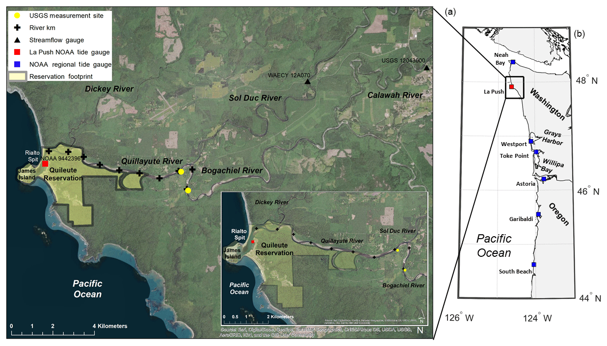
Figure 1Map of study area (a), which is denoted on the regional map (b) in the black box. The La Push tide gauge is represented as a red square while other regional tide gauges are represented as blue squares. The Calawah and Sol Duc River gauges are represented as black triangles, and USGS measurement sites from the May 2010 survey (see information in the Supplement) are depicted as yellow circles. Approximate river kilometers are denoted as black crosses on the study area map.
The Quillayute River is a natural, unstabilized river that is relatively straight at the confluence of the Bogachiel and Sol Duc rivers and increases in sinuosity moving towards the river mouth. Channel-bed materials are coarse (gravel and cobble) in the free-flowing channels and dominated by sand in the small estuary (Czuba et al., 2010). Upstream of river kilometer 3 there are numerous point bars and bends in the river. Between river kilometer 1.5 and 3, the Quillayute River is braided with several side channels, usually containing woody debris (Czuba et al., 2010). The channel is straight near the river mouth and is confined by the Rialto Spit revetment before draining into the Pacific Ocean.
The oceanic climate of the coastal Pacific Northwest (PNW) is cool and wet with a small range in temperature variation and the majority of rainfall between October and May. Four river basins, the Sol Duc, Bogachiel, Calawah, and Dickey rivers, feed into the Quillayute River and comprise the majority of the watershed. Streamflow in the region is primarily from storm-derived rainfall in the winter and snowmelt during the spring and summer (WRCC, 2017).
Oceanographically driven SWLs are generally comprised of mean sea level, tides, and nontidal residuals, which include storm surge. Regional variations in shelf bathymetry, shoreline orientation, storm tracks (Graham and Diaz, 2001), seasonality (Komar et al., 2011), and winds drive differences in storm surge along the US west coast. However, the US west coast's narrow continental shelf, in relation to broad-shelved systems, controls the magnitude of storm surge, which is rarely larger than 1 m (Bromirski et al., 2017; Allan et al., 2011). The PNW is also influenced by a unique interannual climate variability due to the El Niño–Southern Oscillation. During El Niño years, the PNW experiences increased water levels for months at a time, along with changes in the frequency and intensity of storm systems (Komar et al., 2011; Allan and Komar, 2002). In the PNW, tides are micro- and mesotidal, and at La Push the tidal range is mixed, predominantly semidiurnal, with a mean range of 1.95 m and a great diurnal range of 2.58 m (https://tidesandcurrents.noaa.gov/datums.html?id=9442396, last access: October 2017).
Global rise in sea level and local changes in vertical land motions result in significant longshore variations of relative sea level along the Washington coastline. The northern Washington coast is experiencing relative sea level rates of mm year−1 due to a rising coastline, while relative sea level in Willapa Bay in southern Washington is 0.94±2.14 mm year−1 (Komar et al., 2011). Tide gauge records at La Push are too short to calculate robust trends in sea level; however, sea level is likely rising in this location rather than falling, partly due to local land subsidence (Miller et al., 2018).
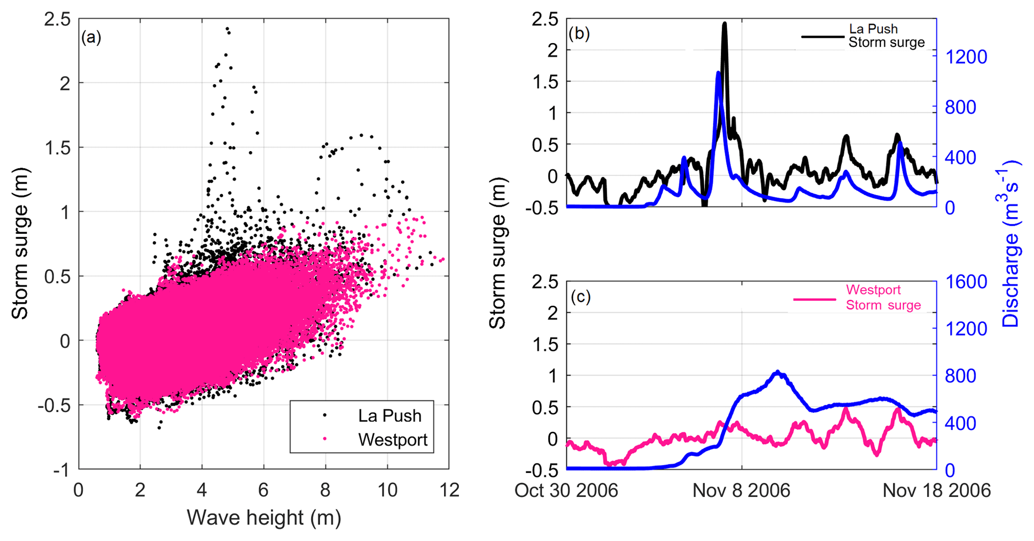
Figure 2(a) The joint relationship between storm surge and wave height for La Push, Washington (black); and Westport, Washington (pink). Example storm surge and discharge relationship at (b) La Push and (c) Westport, Washington.
Observational records in the region are generally sparse; one tide gauge exists in the marina near the river mouth and only two of the four rivers which feed into the Quillayute watershed are gauged (Fig. 1). The Sol Duc River gauge (WA Dept of Ecology 12A070) is located 12 km upriver from the Quillayute River and measures hourly discharge and stage observations from 2005 to 2014. The second river gauge is located on the Calawah River (USGS 12043000), approximately 25 km upriver from the Quillayute River. The Calawah River flows into the Bogachiel River and has hourly discharge and stage measurements from 1989 to 2016. The hourly record of discharge measurements from the Sol Duc River is 100 % complete, while the Calawah River is 99 % complete. An area scaling watershed analysis (Gianfagna et al., 2015) is undertaken to rectify the discharge by the amount of ungauged watershed. The watershed delineation shows that the Bogachiel, Calawah, Sol Duc, and Dickey rivers account for 24 %, 22 %, 37 %, and 17 % of the total Quillayute River watershed area, respectively. Noting the similar watershed characteristics and proportional watershed areas, the contribution of the Bogachiel River is estimated by scaling the Calawah River discharge measurements by a factor of 2.09. This scaling factor for estimating Bogachiel River discharge is validated by comparing to eight discharge point measurements taken during a US Geological Survey (USGS) survey in 2010 (see Supplement). Discharge for the Quillayute River is estimated by adding together discharge from the Sol Duc and Bogachiel rivers.
Hourly measured SWLs at the La Push tide gauge (NOAA station 9442396, 2004–2016) relative to Mean Lower Low Water (MLLW) are downloaded, transformed into NAVD88, and decomposed into mean sea level (ηMSL), tide (ηA), and nontidal residual (ηNTR). The ηNTR is further decomposed into monthly mean sea level anomalies (ηMMSLA), seasonality (ηSE), and storm surge (ηSS), using methods described in Serafin et al. (2017). Peak ηSS events at La Push are found to be the highest on record compared to all US west coast tide gauge stations (Serafin et al., 2017). Upon further investigation of the ηSS record, a large portion of extreme ηSS events occur during low-wave events (Fig. 2a) and high-river-discharge events (Fig. 2b). This is inconsistent with ηSS in Westport, Washington (Fig. 2a and c), just south of La Push, and with other tide gauges along the US west coast (not shown). It is therefore hypothesized that the anomalously large signal seen in the ηSS is river-induced.
To further investigate the anomalously large ηSS at the La Push tide gauge, the hydrodynamic model ADvanced CIRCculation (ADCIRC, Luettich Jr. et al., 1992) and Simulating Waves Nearshore (SWAN, Zijlema, 2010) model (ADCSWAN; Dietrich et al., 2011) is used to simulate water levels at the tide gauge during a storm event corresponding with the peak river discharge on record occurring on 8 January 2009. ADCIRC is run in 2-D depth-integrated barotropic mode which performs well for calculating water surface elevations during storm events (Weaver and Luettich Jr., 2010). SWAN is run in nonstationary mode on an unstructured grid, allowing for tight coupling to ADCIRC. The model is run with two forcing implementations: one including a full forcing of waves, wind, pressure, streamflow, sea level anomalies, seasonality, and tides and one including only streamflow and tides. Once the river-influenced water level is validated, it is removed from the ηSS signal and saved as a sixth geophysical variable (ηRi; see Supplement for removal technique).
Because of the short length of the La Push tide gauge record, decomposed water levels from the La Push tide gauge are merged with decomposed water levels from the Toke Point tide gauge (NOAA station 9440910) to create a combined water level record with a length of 36 years. Details of this methodology are explained in the corresponding Supplement, as well as in Serafin et al. (2019). Once the two tide gauges are merged, the combined hourly tide gauge record extends from 1980 to 2016 and is 97 % complete.
Return level flood magnitudes, such as the 100-year event, are typically assumed to be driven by a specific forcing event, such as the 100-year rainfall or storm surge. However, for processes driven by multiple dimensions, different sizes and combinations of forcing conditions could potentially generate extreme flood magnitudes. To explore the role of compounding forcings in generating extreme water levels, a hybrid modeling framework is developed by merging a hydraulic model simulating river flow with probabilistic simulations of jointly occurring boundary conditions, in this case SWL and river discharge (Fig. 3). Statistical simulations allow for long, synthetic records of joint forcings that may not have occurred in the short observational records but are physically capable of co-occurring. Modeling all of the statistically simulated boundary conditions in a hydraulic model to output along-river water levels would be prohibitively expensive. As an alternative to time-consuming simulations, surrogate models (Razavi et al., 2012) are developed to approximate the response of a hydraulic model simulation at each along-river location. This technique allows for the analysis of along-river water levels driven by a variety of boundary conditions. Long synthetic records on the order of 500 years allow for the direct empirical extraction of water level return levels rather than an extrapolation from historic observational forcing conditions. In addition, the large sample space of simulated variables permits a comparison of event-based return levels, where the 100-year water level is determined by the 100-year forcing, to response-based return levels, where the 100-year water level is derived and then mapped to its respective forcing conditions. This novel framework is flexible for input of any statistical or hydraulic model. In this application, we use the Serafin and Ruggiero (2014) full simulation total water level model and the US Army Corps of Engineers' (USACE) Hydrologic Engineering Center's River Analysis System (HEC-RAS; Brunner, 2016), which are described in more detail below.
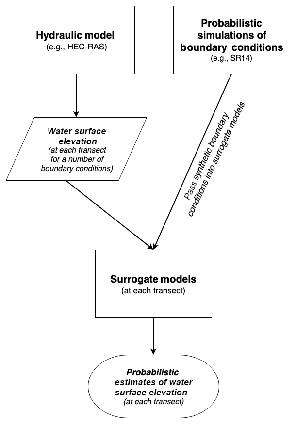
Figure 3Schematic of hybrid statistical–physical modeling technique. Models are portrayed as squares, while circles portray model outputs.
4.1 Probabilistic simulations of boundary conditions
The nonstationary, probabilistic simulation model of Serafin and Ruggiero (2014) (hereinafter SR14) was developed to produce synthetic time series of daily maximum total water levels (TWLs), the combination of waves, tides, and nontidal residuals, on open-coast sandy beaches. SR14 simulates the individual components of the TWL in a Monte Carlo sense, while appropriately accounting for any dependencies existing between the variables. This modeling technique is able to include nonstationary processes influencing extreme and nonextreme events, such as seasonality, climate variability, and trends in wave heights and water levels. SR14 outputs a number of synthetic records of all variables driving TWLs that produce alternate, but physically plausible, combinations of waves and water levels along an identified stretch of coastline. This technique is flexible to allow for both (i) the simulation of the present-day climate for computing robust statistics on extreme TWL events and (ii) the simulation of future climates and their impact on extreme TWLs. Because SR14 was developed for use in open-coast environments, it does not include a procedure for simulating estimates of river discharge, which is present in the local tide gauge at the La Push study site. SR14 is therefore modified to produce synthetic time series of river discharge as well as a river-induced water level.
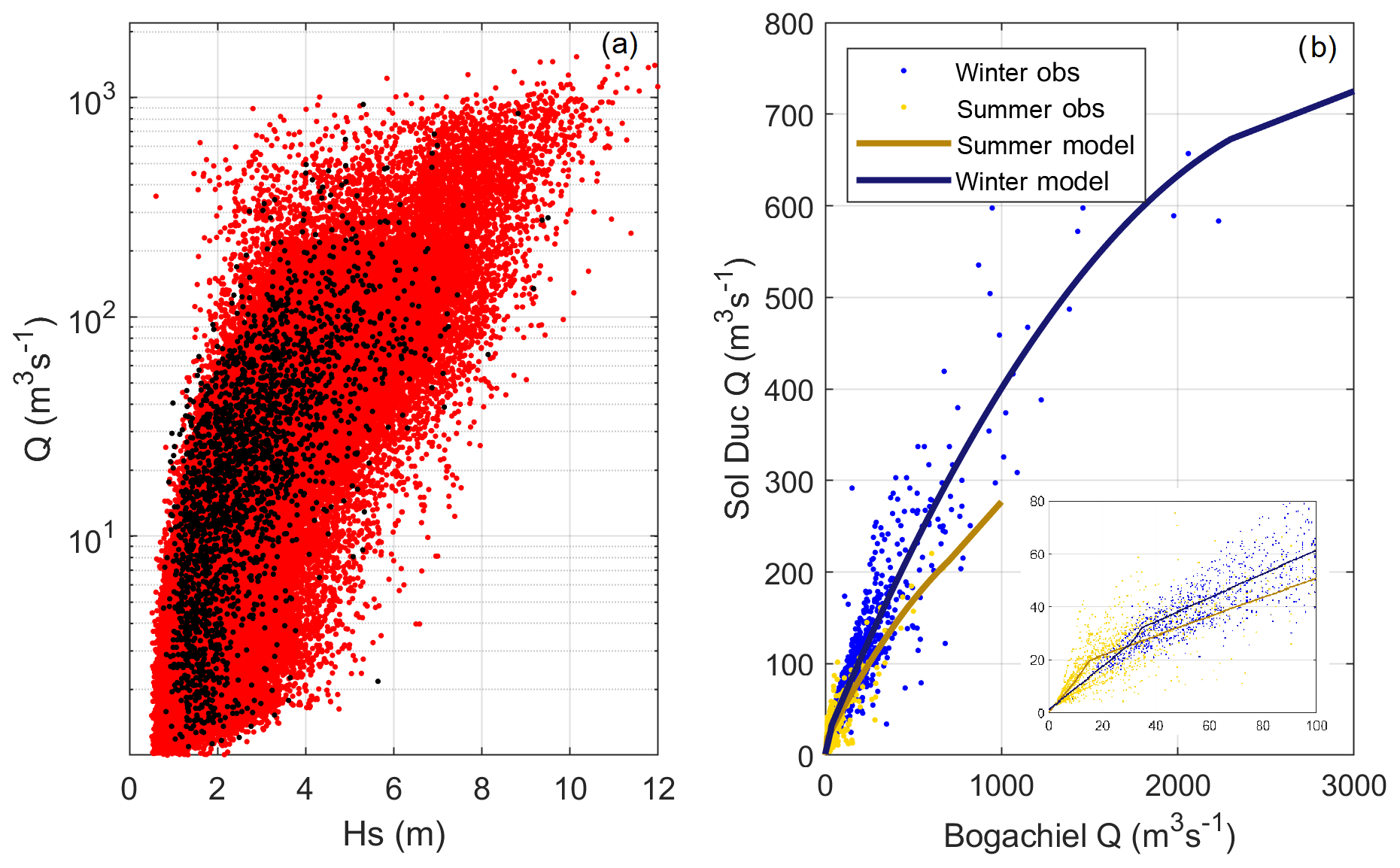
Figure 4(a) Joint relationship between wave height (Hs) and discharge (Q) for the observational record (black) and one example 500-year simulation (red). (b) Seasonal model fit for the probabilistic simulation of the Sol Duc River Q in relation to the Bogachiel River Q. The inset displays the model fits for discharge less than 100 m3 s−1.
High-discharge events on the two gauged rivers in the watershed, the Sol Duc and Calawah rivers, tend to occur within hours of peak wave events recorded in offshore wave buoy records and water level events recorded in the tide gauge data. Due to the interrelated nature of these forcings, daily maximum estimates of Calawah River discharge (QC) are compared to all variables simulated in the SR14 model (e.g., wave height, ηSS, ηNTR, ηMMSLA) to capture any dependencies between these processes. The variable with the highest monthly correlation to QC is wave height (Hs). Extreme QC events are simulated using a bivariate logistic model, which is the same technique used to simulate ηSS. The bivariate logistic model preserves the dependency and frequency of occurrence of joint Hs−Q events in extreme and nonextreme space. This technique generates a synthetic record of QC that is seasonally varying, related to larger-scale climate variability through wave height (essentially as a proxy for storms), and carries the same dependency between variables as the observational record (Fig. 4a). QC is then multiplied by 2.09 to represent inflow from both the Bogachiel and Calawah rivers.
Discharge measurements at the Sol Duc River are highly correlated with the discharge measurements at the Calawah River (ρ=0.9, τ=0.83); thus Sol Duc River discharge (QSD) is modeled based on a relationship with the scaled QC, representing the Bogachiel River (QB). Estimates of QSD are related to QB during the summer and winter seasons. First, daily maximum Q is split into summer (May, June, July, August, September, and October) and winter (January, February, March, April, November, and December) seasons. Next, models are fit to the joint relationship between the QSD and QB each season, such that for the summer season,
is used when QB falls between 0 and 10 m3 s−1, and
is used when QB falls between 10 and 700 m3 s−1 (Fig. 4b). When QB is greater than 700 m3 s−1, QSD is determined using
For the winter season,
is used when QB falls between 0 and 25 m3 s−1, and
is used when QB falls between 25 and 2300 m3 s−1 (Fig. 4b). When QB is greater than 2300 m3 s−1, QSD is determined using
Summer and winter QB is binned and residuals of QSD from the above model fits are generated. Normal distributions are fit to QSD residuals in each bin, except for low bins (less than 25 m3 s−1) where residuals are fit to exponential distributions. QSD is then directly related to simulated estimates of QB; QSD is first determined by fitting the prescribed model to each estimate of QB, and then a random sample is taken from the residuals per binned QB and added to the model. This technique captures the joint peaks of the river systems visible in the observed dataset, while allowing for variability between the simulated estimates (Fig. 4b).
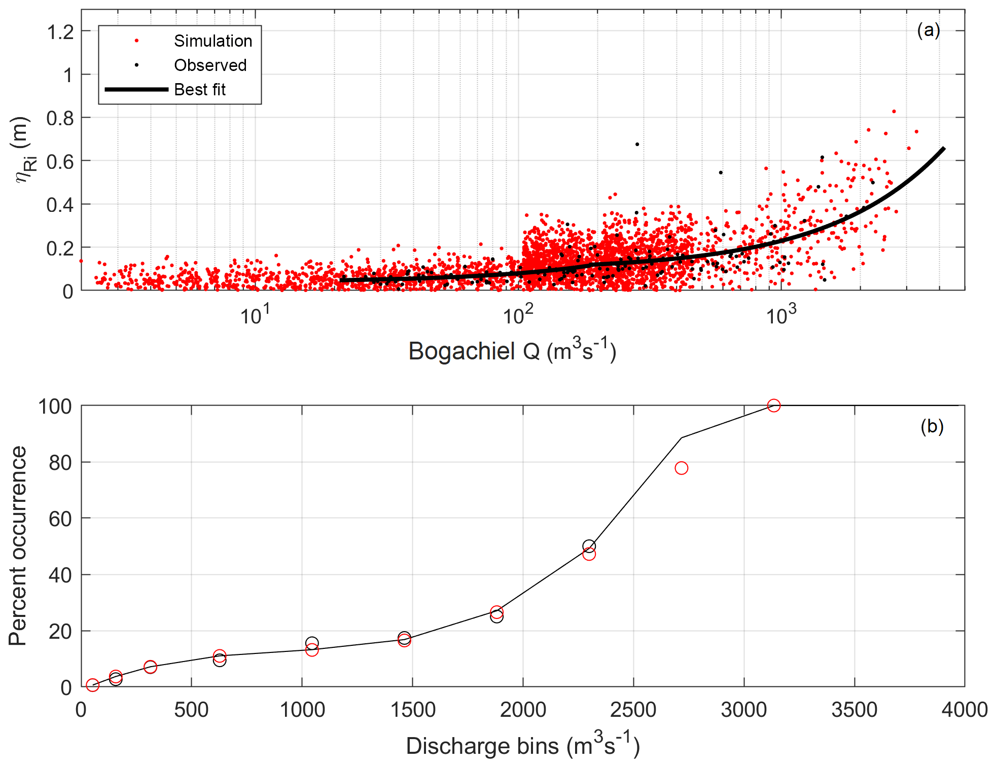
Figure 5(a) The relationship between the river-influenced water level (ηRi) and Bogachiel River discharge on a log-linear scale. The solid black line represents the model fit to the observational records (black dots). (b) The percentage of time ηRi occurs in the record during a specific QB. In both panels, black represents the observational record and red represents one example 500-year simulation.
4.1.1 Modeling the river-induced water level
At tide gauges along the US west coast, the maximum daily SWL generally occurs during, or close to, the daily high tide (Serafin and Ruggiero, 2014; Serafin et al., 2017). Modeling peaks in ηRi that occur during low tide would therefore erroneously increase simulated estimates of the SWL occurring during high tide. Thus, instances of ηRi occurring approximately during high tide are retained and all other ηRi peaks are discarded, resulting in 155 ηRi events.
Synthetic estimates of ηRi are developed by relating QB and ηRi. This relationship is modeled using
when QB is below 190 m3 s−1 and
when QB is above 190 m3 s−1 (Fig. 5a). Next, coarse bins ranging from 100 to 4000 m3 s−1 are created and the standard deviation (σ) of ηRi within each bin is saved. For bins that contain less than 10 observations, observations from the previous bins are included until there are more than 10 observations per bin for σ calculations. Finally, a two-point running average is used to smooth σ from each bin to ensure continuous transitions and to avoid the edge effects from binning a sparse dataset.
There are times of high QB without a distinguishable ηRi in the tide gauge record; thus a model is also developed to simulate the frequency of occurrence of ηRi during daily maximum SWLs. The frequency of occurrence of ηRi is defined as the percentage of time ηRi occurs in the observational record, which is less than 10 % of the time when QB is less than 840 m3 s−1 and 10 %–25 % of the time when QB is between 840 and 2090 m3 s−1 (Fig. 5b). For QB greater than 2090 m3 s−1, ηRi occurs approximately 50 % of the time. The frequency of occurrence of ηRi is modeled using a best-fit cubic function, where the frequency of occurrence is a function of QB based on the percentage of time the values have occurred in the record. Because there are no events greater than 2500 m3 s−1 on record, we represent the percentage of occurrence over this value as 100 % (Fig. 5b).
Once QB is simulated using SR14, ηRi is simulated for every day in time by selecting the synthetic daily estimate of QB and randomly sampling from a normal distribution for each QB bin, where μ is the regression model and σ is the standard deviation from each bin (Fig. 5a). The frequency-of-occurrence model is then used to select the correct proportion of ηRi events to retain for each synthetic simulation. These techniques capture both the spread of ηRi related to QB and the percentage of time of occurrence (Fig. 5).
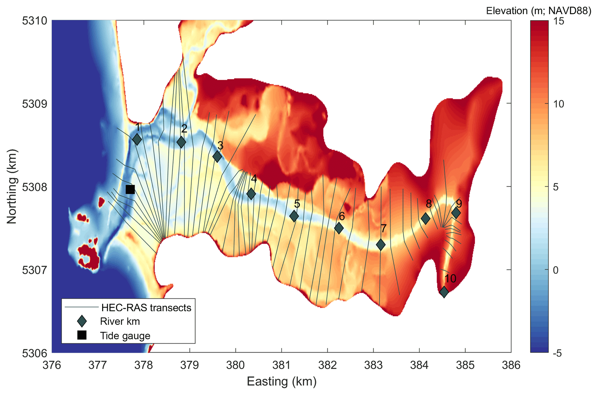
Figure 6Digital elevation model (DEM) used for the HEC-RAS simulations of the Quillayute River. HEC-RAS cross sections are depicted as grey lines. Approximate river kilometer and the location of the tide gauge are depicted as diamonds and a square, respectively.
4.2 Hydraulic model for along-river water levels
While a variety of hydraulic models can be used for determining the elevation of along-river water levels, we employ the Hydraulic Engineering Center's River Analysis System (Brunner, 2016). HEC-RAS is used to estimate water surface elevations in rivers and streams in both steady and unsteady flow and under subcritical, supercritical, and mixed flow regimes (Goodell, 2014). HEC-RAS has been previously used to model water surfaces for a range of applications including, but not limited to, floodplain mapping (Yang et al., 2006), flood forecasting (Saleh et al., 2017), dam breaching (Butt et al., 2013), and flood inundation (Horritt and Bates, 2002). HEC-RAS computes water levels by solving the 1-D energy equation with an iterative procedure, termed the step method, from one cross section to the next (Brunner, 2016). For subcritical flows, the step procedure is carried out moving upstream; computations begin at the downstream boundary of the river and the water surface elevation at an upstream cross section is iteratively estimated until a balanced water surface is obtained. Energy losses between cross sections are comprised of a frictional loss via the Manning equation and a contraction/expansion loss via a coefficient multiplied by the change in velocity head (see Brunner, 2016, for more details).
In this application, HEC-RAS is used to model 1-D water levels under gradually varied, steady-flow conditions at transects along the Quillayute River. While a simplification of flood processes, the 1-D application is commonly used to create flood hazard maps. A detailed digital elevation model (DEM) is developed for the river network, including bathymetry and topography for the floodplains of interest (Fig. 6). Model domain boundary conditions are chosen as the SWL at the tide gauge (m; downstream boundary) and river discharge from the Sol Duc and Bogachiel rivers (m3 s−1; upstream boundary). The HEC-RAS model is validated using water surface measurements from a 2010 survey. Details of the HEC-RAS model validation and calibration procedures are documented in the Supplement.
4.3 Hybrid statistical–physical modeling
The modified simulation technique of SR14 is used to produce 70 500-year-long synthetic records representing present-day climate for the time period of 1980–2016 of daily maximum SWL and Q for both the Sol Duc and Bogachiel rivers. Rather than run the ∼13 million simulated conditions through a numerical model, a limited set of joint boundary conditions of SWL and Q (at the Bogachiel and Sol Duc rivers) are run through HEC-RAS, outputting the elevation of the along-river water level at each HEC-RAS transect. Surrogate models are generated from the HEC-RAS runs for each transect using a scattered linear interpolation of the 3-D surface of boundary conditions. The number of combinations of SWL and Q used to develop the surrogate models are chosen to minimize interpolation errors during validation runs. A daily estimate of water level elevation at each transect is produced by inputting all daily maximum SWL and Q conditions into the surrogate models, which efficiently extract along-river water levels for any set of SWL and Q inputs. Using the count-back method, where for example the fifth largest event for each synthetic record would be the 100-year event, water level return levels are extracted for all 70 500-year synthetic records for the (1) along-river water levels at each transect, (2) SWLs, and (3) Q. This methodology provides both an estimate of the return level magnitude (e.g., the average of the 70 100-year events) and the uncertainty around that magnitude (e.g., the distribution of the 70 100-year events). It also provides a technique to compare the response-based return level (e.g., the 100-year water level) to the event-based return level (e.g., the water level driven by the 100-year SWL or 100-year Q event).
The following section first validates the presence of a river-induced water level within the tide gauge signal and then demonstrates the effectiveness of the surrogate models in representing along-river water levels for unmodeled HEC-RAS boundary conditions. Next, the spatial and temporal variability of the magnitude of along-river water levels and their driving conditions are examined. Finally, low-probability water levels, like the 100-year event, are extracted from the simulated records of along-river water levels, and the dominant drivers are evaluated.
5.1 River-induced water level validation
Results from ADCSWAN modeling of the 8 January 2009 storm event show that the simulation including only river discharge and tides is nearly able to recreate the measured peak ηSS signal at the tide gauge (Fig. 7a). The addition of wind, pressure, waves, sea level anomalies, and seasonality is found to have minimal impact on the peak observed ηSS. Furthermore, the maximum ηSS occurs during low tide (Fig. 7b), which indicates a potential relationship between water surface elevation, tidal level, and river discharge. While the ADCSWAN runs only explore one instance of this phenomenon, it provides physics-based evidence that anomalously high ηSS at the La Push tide gauge is likely being driven by large discharge events.
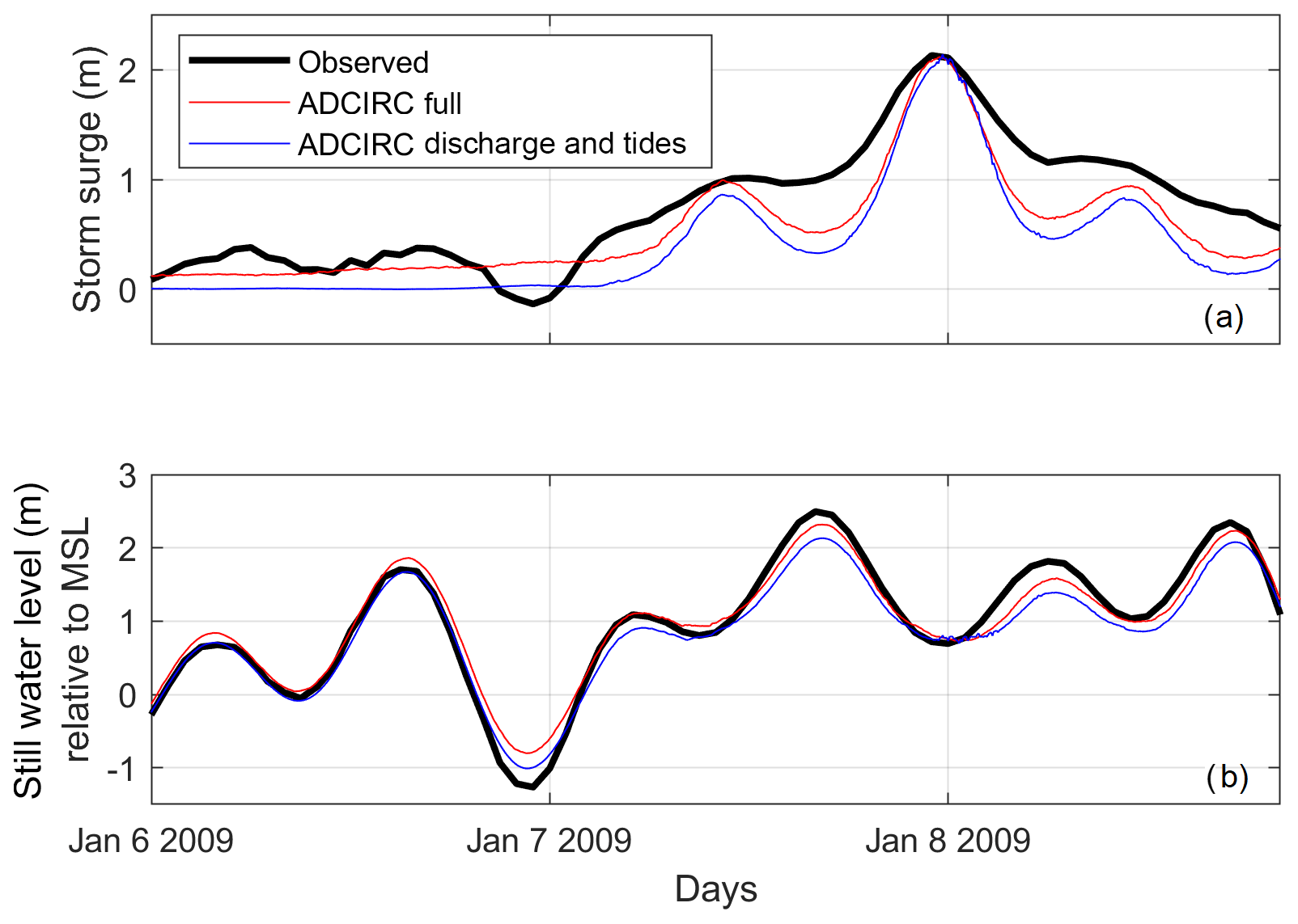
Figure 7Resulting storm surge (a) and still water level (b) at the La Push tide gauge modeled using ADCIRC for a simulation including full forcing (red) and a simulation including only discharge and tides (blue) compared to the observational record (black). The ADCIRC simulation was run for the maximum discharge event on record occurring on 8 January 2009.
5.2 Surrogate model validation
A number of validation scenarios are modeled in HEC-RAS to determine whether the combinations of Q and SWL boundary conditions used to develop the surrogate models represent a large enough sample space of forcing conditions for the interpolation of along-river water levels. The validation scenarios are chosen to cross through both HEC-RAS modeled and unmodeled conditions (Fig. 8a). Across all validation scenarios, the average root mean square error (RMSE) between the HEC-RAS directly modeled and the surrogate model-interpolated water levels is 1 cm. Only 1.5 % of the validation scenarios have a bias greater than 10 cm, and the largest RMSE at any transect is 20 cm across all scenarios (Fig. 9). The validation scenario with the worst performance occurs during high QB and low QSD paired with low-SWL events. However, even during the worst-performing case, the difference between the HEC-RAS directly modeled water level and the surrogate model-interpolated water level is small (Fig. 8b). The main research focus here is extreme water levels, and the conditions driving low-probability return level events rarely fall around the scenarios with the highest bias.
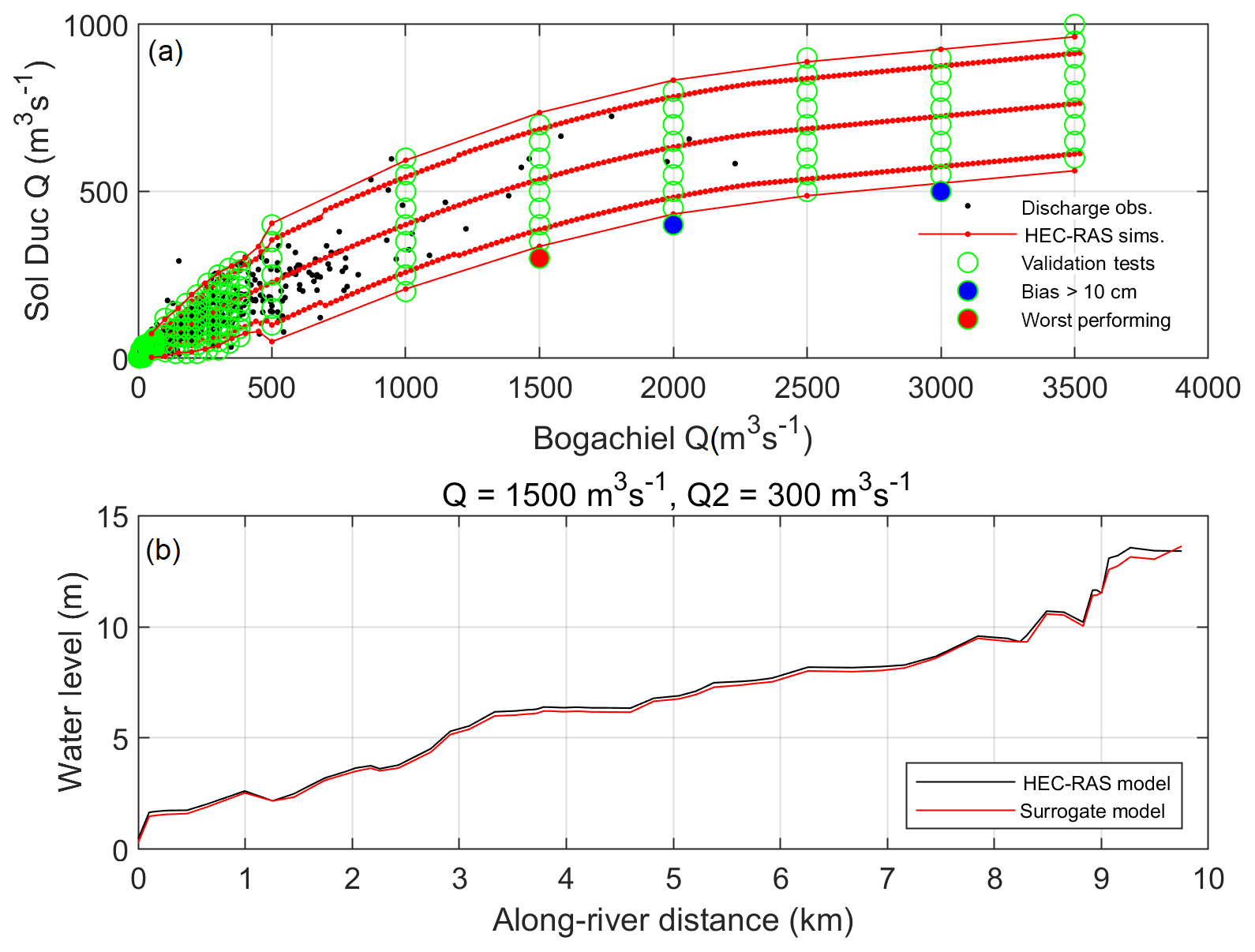
Figure 8(a) Modeled HEC-RAS Q boundary conditions used to generate the surrogate models (red-dotted lines) compared to the simulated conditions used for surrogate model validation (green dots). The black dots represent the observational daily max conditions, while the colored circles represent the worst performing of the validation tests. The red and blue colored circles represent the scenarios where the interpolated water surface had a bias of over 10 cm lower than the model. (b) Example along-river water level for the worst-performing condition in the validation tests.
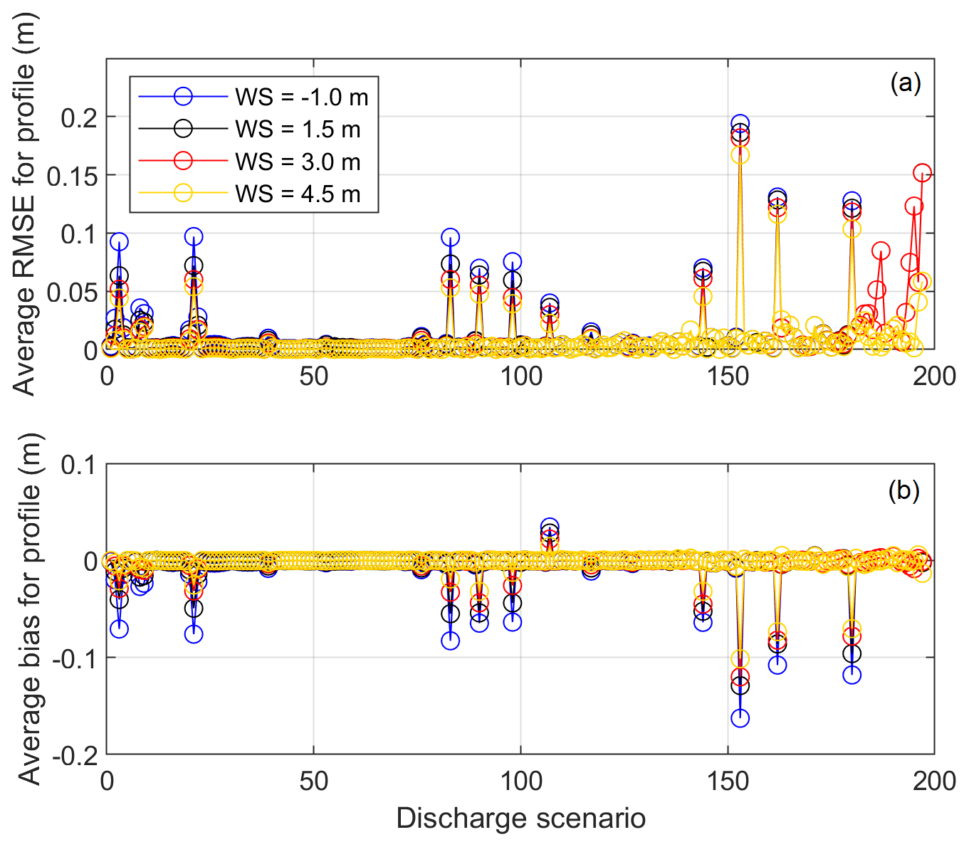
Figure 9(a) Average root mean square error (RMSE) and (b) bias for all 197 discharge validation scenarios across 4 out of the 15 SWL scenarios. The worst-performing model is discharge scenario 153.
5.3 Hybrid modeling of along-river water levels
5.3.1 Temporal variability
Seasonal variability exists in the elevation of along-river water levels. The highest elevation water level occurs during the winter (here defined as December, January, February), while the lowest elevation water level occurs during the spring (March, April, May) (Fig. 10a). The spring along-river water level is on average 0.50 m lower than the winter along-river water level, 0.33 m lower than the fall (September, October, November) along-river water level, and 0.03 m lower than the summer (June, July, August) along-river water level (Fig. 10b). The difference between seasonal along-river water levels is nonlinear upstream, and certain sections of the river have larger changes in elevation between months (Fig. 10b). However, this variation becomes relatively linear downstream of river kilometer 3.
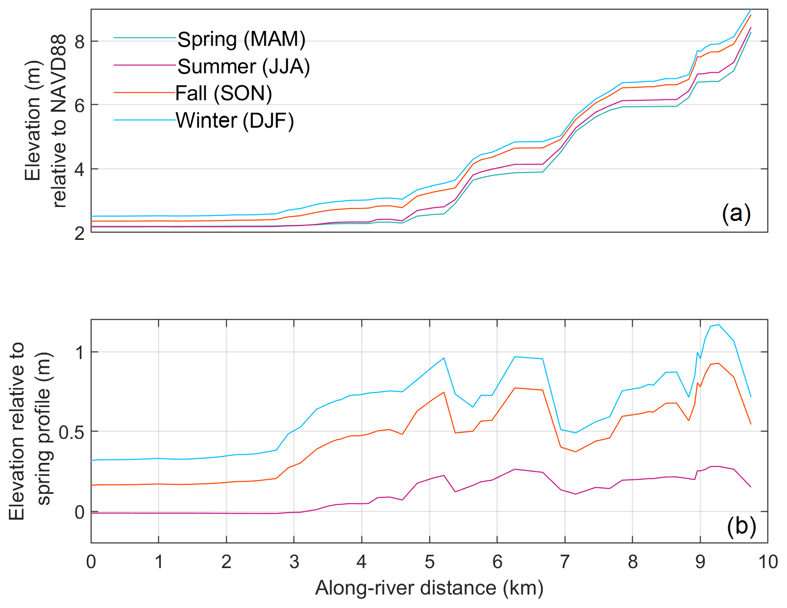
Figure 10(a) Variability of along-river water levels averaged over spring (MAM), summer (JJA), fall (SON), and winter (DJF). (b) The difference between the spring and summer, fall, and winter along-river water levels.
The seasonal variability of the along-river water level is driven by the seasonality of the forcings, which are well represented in the simulations compared to the observations (Fig. 11). The monthly median SWLs and ηNTR's are higher in the winter than in the summer (Fig. 11a and b). This cyclical variability is also depicted in the monthly median river discharge from the Quillayute River (combined Sol Duc and Bogachiel Q) and is approximately 200 m3 s−1 higher in winter months than summer months (Fig. 11c). The 98th percentile values of SWL, ηNTR, and Q have a similar seasonal variability to the median conditions (Fig. 11d–f).
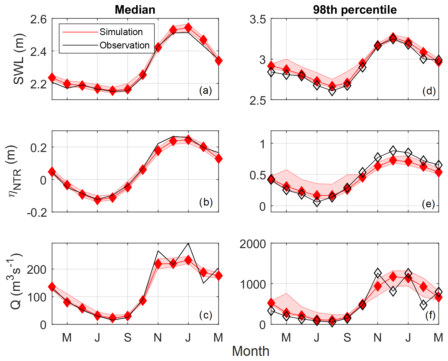
Figure 11(a–c) Observational (black) and simulated (red) monthly median still water level (SWL), nontidal residual (etaNTR), and discharge (Q). (d–f) Observational (black) and simulated (red) monthly 98th percentile of the SWL, ηNTR, and Q. Red shading indicates the bound from each simulation.
5.3.2 Spatial variability
The large number of joint SWL and Q conditions allows for the direct extraction of water level return levels and the corresponding univariate or multivariate drivers along each HEC-RAS transect. The magnitude of the 100, 25, 10, and annual return level water levels is between 3 and 17 m (NAVD88, Fig. 12a). While the peaks in return level events occur at similar locations, the difference between return level events varies spatially moving upriver. For example, at river kilometer 1, the difference between the average (of all simulations) annual and 100-year event is approximately 0.9 m, whereas at river kilometer 8 and upstream, the difference between these two events is closer to 2 m (Fig. 12b).
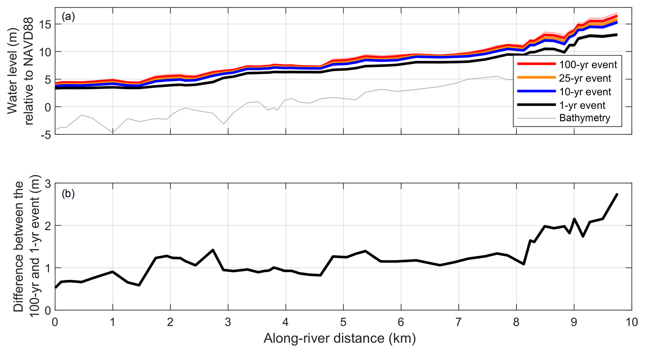
Figure 12(a) The water level return level at each transect for all 70 probabilistic simulations. Each return level event displays the average of the simulations (solid line) as well as the range around the average (shaded). (b) The along-river difference between the annual and 100-year event, averaged over 70 simulations.
The dominant forcing conditions driving water level return levels vary along-river. At the river mouth, the annual water level event (e.g., the event that is expected every year) in each simulation occurs during Q ranging from 40 to 2600 m3 s−1 and SWLs around 3.3 m, which corresponds with the annual SWL event (Fig. 13a). Moving upstream to river kilometer 1 and 2, the annual water level event is driven by both high SWL occurring during low Q and low SWL occurring during high Q. At river kilometer 4, the annual water level event occurs during the annual Q event coincident with SWLs that range from 1.8 to 3.9 m (Fig. 13a). These results are similar, albeit events are larger magnitude, for the 100-year water level event. Downstream 100-year water levels are driven by SWLs, upstream 100-year water levels are driven by Q, and the 100-year water level between kilometer 1 and 2 is driven by different combinations of high- and low-SWL and Q events (Fig. 13b).
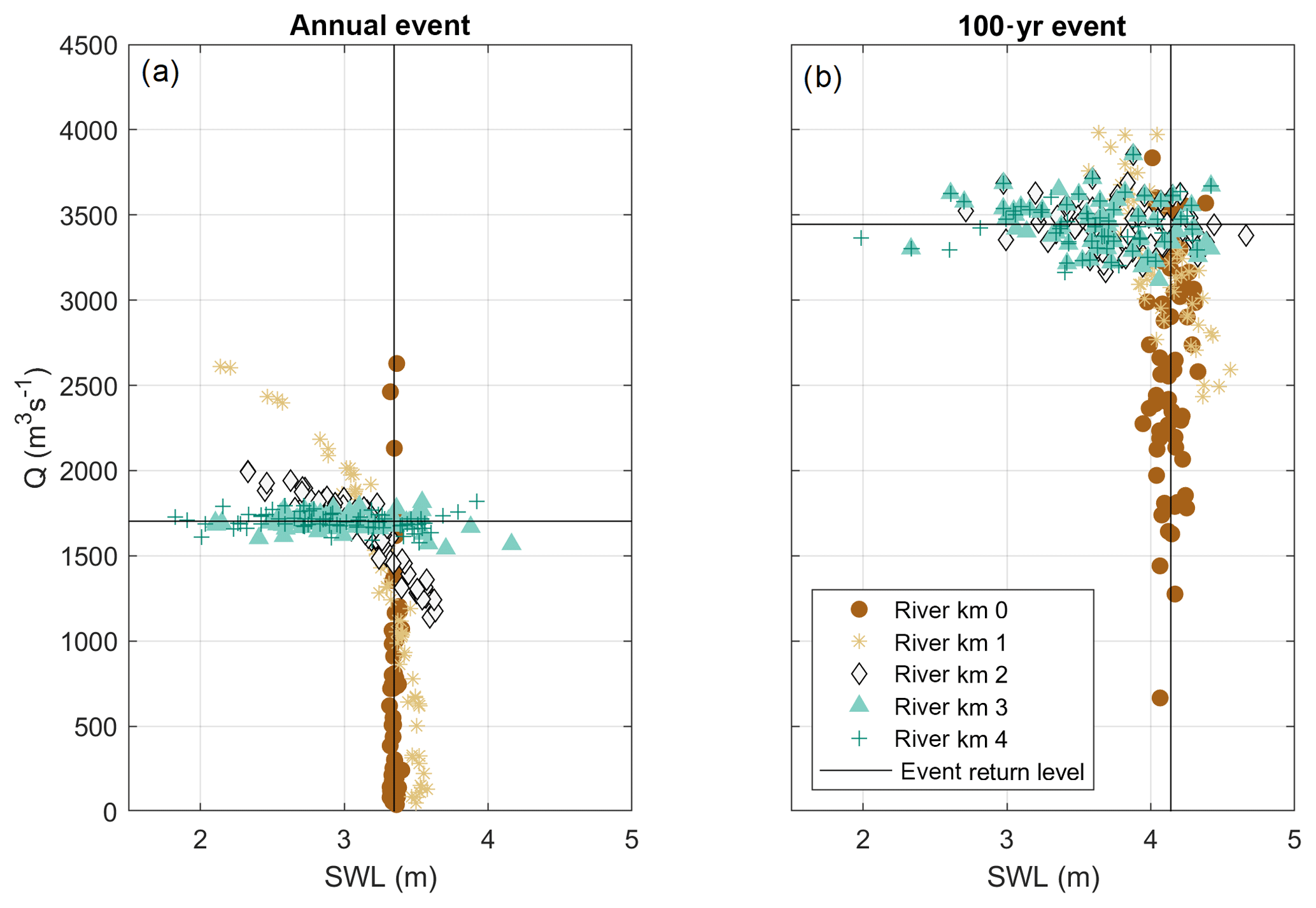
Figure 13The individual Q or SWL condition driving the (a) annual and (b) 100-year water level event at specific along-river locations for each 70 500-year simulation. In both figures, the black lines represent the annual and 100-year return level magnitude for Q and SWL.
The relative importance of both oceanic and riverine forcing to extreme water levels emerges when averaging the magnitude of the drivers of the water level return levels at each transect from all 70 500-year-long simulations (Fig. 14). The magnitude of the average Q driving water level return levels gradually increases by approximately 1000 m3 s−1 over river kilometer 0–2 and then is consistent from river kilometer 2 to 10 (Fig. 14a). Downstream, between river kilometer 0 and 0.25, the magnitude of the average SWL driving water level return levels is consistent and then gradually decreases over a 1 km zone (Fig. 14b).
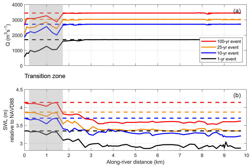
Figure 14The average forcing condition driving along-river return levels at each transect where (a) displays the Quillayute Q conditions and (b) displays the SWL conditions. The dashed lines depict the univariate forcing conditions, where the along-river return level is assumed to be driven by either Q or SWL. Red, orange, blue, and black lines represent the 100, 25, 10, and annual return level event. The grey shaded area represents a transition zone, where the water level is driven by a combination of SWL and Q events.
When comparing to water level return levels driven by a univariate forcing or event return level (e.g., along-river water levels modeled from the 100-year Q or SWL event), we find that the stretches of river driven by a consistent SWL or Q forcing approximate the univariate return level event. Therefore, the 100-year SWL does indeed cause the 100-year water level downstream, between river kilometer 0 and 0.25, while the 100-year Q event drives the 100-year water level upstream, between river kilometer 2 and 10 (dashed lines, Fig. 14). However, between river kilometer 0.25 and 1.75 a flood transition zone is present, where neither the SWL return level or the Q return level events drive the water level return level. This is consistent across all return level events.
The hybrid model developed in this study, which combines statistical simulations with a physics-based model, provides an approach for probabilistically evaluating the conditions that drive extreme water levels not only in an open-coast setting, but also kilometers upriver. The ability to simulate millions of combinations of Q and SWL events allows for a robust estimate of resulting along-river water levels, which numerical models alone are unable to consider due to large computational expenses. While some of our modeling techniques are specific to this location, the overall framework for combining statistical and physics-based models is general enough for use in coastal locations throughout the globe where flooding arises from compounding processes.
The decomposition of the SWL into low- and high-frequency signals, including a river-influenced component, helps identify the importance of physical processes for generating high water levels across various regional settings. This is especially important in locations like the US west coast, where the steep, narrow continental shelf prevents wind- and pressure-driven storm surge from being overwhelmingly large (Allan et al., 2011). The influence of the river signal in the tide gauge is directly related to the setting of our study site. The estuary is relatively small and narrow with the river discharging directly into the ocean. This is dissimilar to other tide gauges in the region which are located in larger estuaries, situated away from river input. Estuaries typically exhibit wave, tide, or river-dominant morphology, based on the relative energy of each process (Dalrymple et al., 1992). The Quillayute River outlets directly to a high-wave-energy environment and has a small estuary volume compared to its river input volume. The steep catchment of the mountainous environment means a short response time for rainfall, therefore producing peak discharges temporally similar to peak storm-induced still water levels, allowing for interaction between the two. In contrast, water level elevations with large estuary volume compared to river discharge are less influenced by fluvial processes. Furthermore, a larger estuary may experience variability in the water surface elevation due to wave-induced setup and/or other local storm-induced processes (Cheng et al., 2014; Olabarrieta et al., 2011), which may further dampen the influence of a river signal.
This research confirms the presence of an oceanographic–fluvial transition zone, where traditional, univariate methodologies for defining return level events are insufficient for defining water level return levels. Between river kilometer 1 and 2, we find that a range of SWL and Q conditions drive all return level events, and water levels are driven by neither the univariate SWL or Q return level event. A similar flood zone transition was recently modeled numerically and, albeit for a single event, physically demonstrates the importance of including multiple variables to reproduce accurate flooding (Bilskie and Hagen, 2018). Thus, flood hazard assessments on systems with multivariate forcings may misrepresent water level elevations for low-probability events if only univariate variables are modeled. This has large implications for characterizing the risk to flooding, especially in the context of mapping flooding hazards. Furthermore, we show that return level water levels can occur over a range of combined extreme and nonextreme forcing in the flood transition zone. This illustrates that, in order to properly understand the impacts of compounding flooding, more than just design scenarios need to be considered for the proper assessment of risk.
Many of our results can be explained by dynamics that occur during interacting ocean and river flows. For example, a coincidence of high SWL and peak river discharge may induce blocking, where river-induced water levels are trapped upstream and either flood overbank or outlet to the ocean as the tide recedes (Kumbier et al., 2018; Chen and Liu, 2014). The outletting to the ocean as the tide recedes artificially inflates SWLs at the tide gauge, increasing water levels for days at a time and prolonging exposure to flooding. When subtracting a tide time series from this signal, storm surge would appear to be elevated at low tide. While the ADCSWAN simulation confirms the presence of this effect by matching the peak storm surge at low tide, our hybrid methodology only models steady-flow scenarios. Thus, with co-occurring daily maximum SWL and discharge, our model may miss certain dynamics important for flooding over unsteady conditions. Furthermore, interactions between storm surge and river discharge may increase the overall elevation of the residual (Maskell et al., 2013). While beyond the scope of our present study, these unsteady characteristics are important to consider in future research.
Because sea level rise, along with other changes to the climate, will exacerbate the compounding effects of flood drivers (Moftakhari et al., 2017; Wahl et al., 2015), it is also important to consider the impact of changes to processes driving flooding events in the future (Zscheischler et al., 2018). By 2100, the likely range of relative sea level rise in the La Push area is projected to be between 18 and 80 cm, considering vertical land motion and various emissions scenarios (Miller et al., 2018). The western Olympic Peninsula is projected to experience increased winter precipitation (Mote et al., 2013; Halofsky et al., 2011), which could subsequently increase either the frequency or intensity of high-Q events along the Quillayute River. While we have characterized the spatial variability in extreme water levels in the present day, there is a high likelihood changes in the future climate will shift the importance of these interacting processes.
This research illustrates the importance of considering a large number of forcing conditions to model compounding processes when evaluating extreme water levels. Here we find that, in coastal settings, river discharge can be an important driver of high water levels measured in a tide gauge. We also find that the univariate, event-based return level event, like the 100-year discharge, does not always match the response-based return level, like the 100-year water level. Furthermore, when processes compound, along-river return levels may be driven by events that are not considered extreme themselves. Probabilistic techniques allowing for the analysis of thousands to millions of combinations of events not captured in the observational record provide a characterization of where river, ocean, or the combination of the two may be important for generating extreme events.
Overall, the hybrid merging of a statistical and numerical model provides a methodology for better understanding the drivers of flooding along the length of a river. While our model does not actively resolve the physical interaction of river and oceanographic flow, it develops an approach for characterizing and extracting river-influenced water levels measured at tide gauges while robustly modeling the drivers of extreme along-river water levels. Understanding the dominant, spatially variable drivers of flooding events will help coastal communities better understand their risks, which is important for increasing resilience to future events.
Data can be made available by the authors upon request.
The supplement related to this article is available online at: https://doi.org/10.5194/nhess-19-1415-2019-supplement.
The study and methodology were conceived by KAS and PR. KAS carried out the analyses, produced the results, and wrote the manuscript under the supervision of PR. KP carried out the analyses and produced the results of the ADCIRC simulations. KP also developed the topography/bathymetry DEM as well as the geometric files for use in HEC-RAS. KAS, PR, KP, and DFH all contributed by generating ideas, discussing results, and editing the manuscript.
The authors declare that they have no conflict of interest.
Tide gauge records are available through the National Oceanic and Atmospheric Administration (NOAA) National Ocean Service (NOS) website, and river discharge is available through the US Geological Survey (USGS) National Water Information System (https://waterdata.usgs.gov/wa/nwis/rt, last access: October 2017). Bathymetric and topographic data for DEM creation were obtained from NOAA's elevation data viewer. Thank you to Michael Rossotto and Garrett Rasmussen for providing updated shapefiles of the Quileute Reservation boundaries. Thank you also to two anonymous reviewers whose comments improved the quality of this paper. This work was funded by the NOAA Regional Integrated Sciences and Assessments Program (NA15OAR4310145) and a contracted grant with the Quinault Treaty Area (QTA) tribal governments (Quinault Indian Nation, Hoh Indian Tribe, and Quileute Tribe).
This research has been supported by the NOAA Regional Integrated Sciences and Assessments Program (grant no. NA15OAR4310145).
This paper was edited by Paolo Tarolli and reviewed by Philip Ward and one anonymous referee.
Allan, J. C. and Komar, P. D.: Extreme storms on the Pacific Northwest coast during the 1997–98 El Niño and 1998–99 La Niña, J. Coast. Res., 18, 175–193, 2002. a
Allan, J. C., Komar, P. D., and Ruggiero, P.: Storm Surge Magnitudes and Frequency on the Central Oregon Coast, in: Proc. Solutions to Coastal Disasters Conf., 26–29 June 2011, Anchorage, Alaska, 2011. a, b
Bevacqua, E., Maraun, D., Hobæk Haff, I., Widmann, M., and Vrac, M.: Multivariate statistical modelling of compound events via pair-copula constructions: analysis of floods in Ravenna (Italy), Hydrol. Earth Syst. Sci., 21, 2701–2723, https://doi.org/10.5194/hess-21-2701-2017, 2017. a, b
Bilskie, M. and Hagen, S.: Defining Flood Zone Transitions in Low-Gradient Coastal Regions, Geophys. Res. Lett., 45, 2761–2770, 2018. a, b, c
Bromirski, P. D., Flick, R. E., and Miller, A. J.: Storm surge along the Pacific coast of North America, J. Geophys. Res.-Oceans, 122, 441–457, 2017. a
Brunner, G. W.: HEC-RAS River Analysis System Hydraulic Reference Manual, Version 5.0, Tech. rep., US Army Corps of Engineers, Institute for Water Resources, Hydrologic Engineering Center, Davis, CA, 2016. a, b, c, d
Bunya, S., Dietrich, J. C., Westerink, J., Ebersole, B., Smith, J., Atkinson, J., Jensen, R., Resio, D., Luettich, R., Dawson, C., Cardone, V. J., Cox, A. T., Powell, M. D., Westerink, H. J., and Roberts, H. J.: A high-resolution coupled riverine flow, tide, wind, wind wave, and storm surge model for southern Louisiana and Mississippi. Part I: Model development and validation, Mon. Weather Rev., 138, 345–377, 2010. a
Butt, M. J., Umar, M., and Qamar, R.: Landslide dam and subsequent dam-break flood estimation using HEC-RAS model in Northern Pakistan, Nat. Hazards, 65, 241–254, 2013. a
Chelton, D. B. and Enfield, D. B.: Ocean signals in tide gauge records, J. Geophys. Res.-Solid, 91, 9081–9098, 1986. a
Chen, W.-B. and Liu, W.-C.: Modeling flood inundation induced by river flow and storm surges over a river basin, Water, 6, 3182–3199, 2014. a, b
Cheng, T., Hill, D., and Read, W.: The Contributions to Storm Tides in Pacific Northwest Estuaries: Tillamook Bay, Oregon, and the December 2007 Storm, J. Coast. Res., 31, 723–734, 2014. a
Couasnon, A., Sebastian, A., and Morales-Nápoles, O.: A Copula-Based Bayesian Network for Modeling Compound Flood Hazard from Riverine and Coastal Interactions at the Catchment Scale: An Application to the Houston Ship Channel, Texas, Water, 10, 1190, https://doi.org/10.3390/w10091190, 2018. a
Czuba, J. A., Barnas, C. R., McKenna, T. E., Justin, G. B., and Payne, K. L.: Bathymetric and streamflow data for the Quillayute, Dickey, and Bogachiel Rivers, Clallam County, Washington, April–May 2010, in: vol. 537, US Department of the Interior, US Geological Survey, Reston, Virginia, 2010. a, b, c
Dalrymple, R. W., Zaitlin, B. A., and Boyd, R.: Estuarine facies models: conceptual basis and stratigraphic implications: perspective, J. Sediment. Res., 62, 1130–1146, https://doi.org/10.1306/D4267A69-2B26-11D7-8648000102C1865D, 1992. a
de Vries, H., Breton, M., de Mulder, T., Krestenitis, Y., Ozer, J., Proctor, R., Ruddick, K., Salomon, J. C., and Voorrips, A.: A comparison of 2D storm surge models applied to three shallow European seas, Environ. Softw., 10, 23–42, https://doi.org/10.1016/0266-9838(95)00003-4, 1995. a
Dietrich, J., Zijlema, M., Westerink, J., Holthuijsen, L., Dawson, C., Luettich Jr, R., Jensen, R., Smith, J., Stelling, G., and Stone, G.: Modeling hurricane waves and storm surge using integrally-coupled, scalable computations, Coast. Eng., 58, 45–65, 2011. a
Gianfagna, C. C., Johnson, C. E., Chandler, D. G., and Hofmann, C.: Watershed area ratio accurately predicts daily streamflow in nested catchments in the Catskills, New York, J. Hydrol.: Reg. Stud., 4, 583–594, 2015. a
Goodell, C.: Breaking the HEC-RAS Code: A User's Guide to Automating HEC-RAS, h2ls, Portland, OR, 2014. a
Graham, N. E. and Diaz, H. F.: Evidence for intensification of North Pacific winter cyclones since 1948, B. Am. Meteorol. Soc., 82, 1869–1893, 2001. a
Halofsky, J. E., Peterson, D. L., O'Halloran, K. A., and Hoffman, C. H.: Adapting to climate change at Olympic National Forest and Olympic National Park, Gen. Tech. Rep. PNW-GTR-844, US Department of Agriculture, Forest Service, Pacific Northwest Research Station, Portland, OR, p. 130, 2011. a
Horritt, M. and Bates, P.: Evaluation of 1D and 2D numerical models for predicting river flood inundation, J. Hydrol., 268, 87–99, 2002. a
Horsburgh, K. and Wilson, C.: Tide-surge interaction and its role in the distribution of surge residuals in the North Sea, J. Geophys. Res.-Oceans, 112, 1–13, https://doi.org/10.1029/2006JC004033, 2007. a
Komar, P. D., Allan, J. C., and Ruggiero, P.: Sea level variations along the US Pacific Northwest coast: Tectonic and climate controls, J. Coast. Res., 27, 808–823, 2011. a, b, c
Kumbier, K., Carvalho, R. C., Vafeidis, A. T., and Woodroffe, C. D.: Investigating compound flooding in an estuary using hydrodynamic modelling: a case study from the Shoalhaven River, Australia, Nat. Hazards Earth Syst. Sci., 18, 463–477, https://doi.org/10.5194/nhess-18-463-2018, 2018. a, b
Leonard, M., Westra, S., Phatak, A., Lambert, M., van den Hurk, B., McInnes, K., Risbey, J., Schuster, S., Jakob, D., and Stafford-Smith, M.: A compound event framework for understanding extreme impacts, Wiley Interdisciplin. Rev.: Clim. Change, 5, 113–128, 2014. a
Luettich Jr., R. A., Westerink, J. J., and Scheffner, N. W.: ADCIRC: An Advanced Three-Dimensional Circulation Model for Shelves, Coasts, and Estuaries, Report 1, Theory and Methodology of ADCIRC-2DDI and ADCIRC-3DL, Tech. rep., Coastal Engineering Research Center, Vicksburg, MS, 1992. a
Maskell, J., Horsburgh, K., Lewis, M., and Bates, P.: Investigating River–Surge Interaction in Idealised Estuaries, J. Coast. Res., 30, 248–259, 2013. a
Mawdsley, R. J. and Haigh, I. D.: Spatial and temporal variability and long-term trends in skew surges globally, Front. Mar. Sci., 3, 29, https://doi.org/10.3389/fmars.2016.00029, 2016. a
Miller, I. M., Morgan, H., Mauger, G., Newton, T., Weldon, R., Schmidt, D., Welch, M., and Grossman, E.: Projected Sea Level Rise for Washington State – A 2018 Assessment. A collaboration of Washington Sea Grant, University of Washington Climate Impacts Group, Oregon State University, University of Washington, and US Geological Survey, Prepared for the Washington Coastal Resilience Project, 2018. a, b
Moftakhari, H. R., Salvadori, G., AghaKouchak, A., Sanders, B. F., and Matthew, R. A.: Compounding effects of sea level rise and fluvial flooding, P. Natl. Acad. Sci. USA, 114, 9785–9790, 2017. a, b
Moftakhari, H. R., Schubert, J. E., AghaKouchak, A., Matthew, R., and Sanders, B. F.: Linking Statistical and Hydrodynamic Modeling for Compound Flood Hazard Assessment in Tidal Channels and Estuaries, Adv. Water Resour., 128, 28–38, https://doi.org/10.1016/j.advwatres.2019.04.009, 2019. a
Mote, P. W., Abatzoglou, J. T., and Kunkel, K. E.: Climate: Variability and Change in the Past and Future, in: Climate Change in the Northwest: Implications for Our Landscapes, Waters, and Communities, edited by: Dalton, M. M., Mote, P. W., and Snover, A. K., Island Press, Washington, D.C., 25–40, 2013. a
Odigie, K. O. and Warrick, J. A.: Coherence between Coastal and River Flooding along the California Coast, J. Coast. Res., 34, 308–317, https://doi.org/10.2112/JCOASTRES-D-16-00226.1, 2017. a
Olabarrieta, M., Warner, J. C., and Kumar, N.: Wave-current interaction in Willapa Bay, J. Geophys. Res.-Oceans, 116, 1–27, https://doi.org/10.1029/2011JC007387, 2011. a
Olbert, A. I., Comer, J., Nash, S., and Hartnett, M.: High-resolution multi-scale modelling of coastal flooding due to tides, storm surges and rivers inflows. A Cork City example, Coast. Eng., 121, 278–296, 2017. a
Razavi, S., Tolson, B. A., and Burn, D. H.: Review of surrogate modeling in water resources, Water Resour. Res., 48, 1–32, https://doi.org/10.1029/2011WR011527, 2012. a
Saleh, F., Ramaswamy, V., Wang, Y., Georgas, N., Blumberg, A., and Pullen, J.: A Multi-Scale Ensemble-based Framework for Forecasting Compound Coastal-Riverine Flooding: The Hackensack-Passaic Watershed and Newark Bay, Adv. Water Resour., 110, 371–386, https://doi.org/10.1016/j.advwatres.2017.10.026, 2017. a
Serafin, K. A. and Ruggiero, P.: Simulating extreme total water levels using a time-dependent, extreme value approach, J. Geophys. Res.-Oceans, 119, 6305–6329, 2014. a, b, c
Serafin, K. A., Ruggiero, P., and Stockdon, H. F.: The relative contribution of waves, tides, and nontidal residuals to extreme total water levels on US West Coast sandy beaches, Geophys. Res. Lett., 44, 1839–1847, 2017. a, b, c
Serafin, K. A., Ruggiero, P., Barnard, P., and Stockdon, H. F.: The influence of shelf bathymetry and beach topography on extreme total water levels: Linking large-scale changes of the wave climate to local coastal hazard, Coast. Eng., 150, 1–17, https://doi.org/10.1016/j.coastaleng.2019.03.012, 2019. a
Svensson, C. and Jones, D. A.: Dependence between extreme sea surge, river flow and precipitation in eastern Britain, Int. J. Climatol., 22, 1149–1168, 2002. a
Sweet, W. V., Park, J., Gill, S., and Marra, J.: New ways to measure waves and their effects at NOAA tide gauges: A Hawaiian-network perspective, Geophys. Res. Lett., 42, 9355–9361, 2015. a
Tsimplis, M. and Woodworth, P.: The global distribution of the seasonal sea level cycle calculated from coastal tide gauge data, J. Geophys. Res.-Oceans, 99, 16031–16039, 1994. a
van den Hurk, B., van Meijgaard, E., de Valk, P., van Heeringen, K.-J., and Gooijer, J.: Analysis of a compounding surge and precipitation event in the Netherlands, Environ. Res. Lett., 10, 035001, https://doi.org/10.1088/1748-9326/10/3/035001, 2015. a
Vetter, O., Becker, J. M., Merrifield, M. A., Pequignet, A.-C., Aucan, J., Boc, S. J., and Pollock, C. E.: Wave setup over a Pacific Island fringing reef, J. Geophys. Res.-Oceans, 115, C12066, https://doi.org/10.1029/2010JC006455, 2010. a
Wahl, T., Jain, S., Bender, J., Meyers, S. D., and Luther, M. E.: Increasing risk of compound flooding from storm surge and rainfall for major US cities, Nat. Clim. Change, 5, 1093–1097, 2015. a, b, c
Ward, P. J., Couasnon, A., Eilander, D., Haigh, I. D., Hendry, A., Muis, S., Veldkamp, T. I., Winsemius, H. C., and Wahl, T.: Dependence between high sea-level and high river discharge increases flood hazard in global deltas and estuaries, Environ. Res. Lett., 13, 084012, https://doi.org/10.1088/1748-9326/aad400, 2018. a
Weaver, R. and Luettich Jr., R.: 2D vs. 3D storm surge sensitivity in ADCIRC: Case study of Hurricane Isabel, in: International Conference on Estuarine and Coastal Modeling, 4–6 November 2009, Seattle, WA, 762–779, 2010. a
Williams, J., Horsburgh, K. J., Williams, J. A., and Proctor, R. N.: Tide and skew surge independence: New insights for flood risk, Geophys. Res. Lett, 43, 6410–6417, 2016. a
WRCC: Climate of Washington: Western Regional Climate Center website, available at: https://wrcc.dri.edu/Climate/narrative_wa.php, last access: 3 November 2017. a
Yang, J., Townsend, R. D., and Daneshfar, B.: Applying the HEC-RAS model and GIS techniques in river network floodplain delineation, Can. J. Civ. Eng., 33, 19–28, 2006. a
Zheng, F., Westra, S., and Sisson, S. A.: Quantifying the dependence between extreme rainfall and storm surge in the coastal zone, J. Hydrol., 505, 172–187, 2013. a
Zijlema, M.: Computation of wind-wave spectra in coastal waters with SWAN on unstructured grids, Coast. Eng., 57, 267–277, 2010. a
Zscheischler, J., Westra, S., Hurk, B. J., Seneviratne, S. I., Ward, P.J., Pitman, A., AghaKouchak, A., Bresch, D. N., Leonard, M., Wahl, T., and Zhang, X.: Future climate risk from compound events, Nat. Clim. Change, 8, 469–477, https://doi.org/10.1038/s41558-018-0156-3, 2018. a, b