UAV-based mapping, back analysis and trajectory modeling of a coseismic rockfall in Lefkada island, Greece

We present field evidence and a kinematic study of a rock block mobilized in the Ponti area by a M_w = 6.5 earthquake near the island of Lefkada on 17 November 2015. A detailed survey was conducted using an unmanned aerial vehicle (UAV) with an ultrahigh definition (UHD) camera, which produced a high-resolution orthophoto and a digital terrain model (DTM). The sequence of impact marks from the rock trajectory on the ground surface was identified from the orthophoto and field verified. Earthquake characteristics were used to estimate the acceleration of the rock slope and the initial condition of the detached block. Using the impact points from the measured rockfall trajectory, an analytical reconstruction of the trajectory was undertaken, which led to insights on the coefficients of restitution (CORs). The measured trajectory was compared with modeled rockfall trajectories using recommended parameters. However, the actual trajectory could not be accurately predicted, revealing limitations of existing rockfall analysis software used in engineering practice.

1 Introduction

Active faulting, rock fracturing and high rates of seismicity contribute to a high rockfall hazard in Greece. Rockfalls damage roadways and houses (Saroglou, 2013) and are most often triggered by rainfall and, secondly, seismic loading. In recent years, some rockfalls have impacted archaeological sites (Marinos and Tsiambaos, 2002; Saroglou et al., 2012). The Ionian Islands, which include Lefkada island, experience frequent M_w = 5–6.5 earthquakes, as well as less frequent larger (up to 7.5) earthquakes. The historical seismological record for the island is particularly well constrained with reliable detailed information for at least 23 such earthquake events that induced ground failure since 1612. On average, Lefkada experiences a damaging earthquake every 18 years. In the recent past, a M_w = 6.2 earthquake occurred on 14 August 2003 offshore the NW coast of Lefkada and caused landslides, rockslides and rockfalls along the western coast of the island (Karakostas et al., 2004; Papathanasiou et al., 2012). Significant damage was reported, particularly in the town of Lefkada, where a peak ground acceleration (PGA) of 0.42 g was recorded.

On 17 November 2015, an M_w = 6.5 earthquake struck the island of Lefkada and triggered a number of landslides, rockfalls and some structural damage. The most affected area by large rockslides was the western coast of the island, especially along its central and south portion, which are popular summer tourist destinations (Zekkos et al., 2017). The coseismic landslides completely covered the majority of the west coast beaches and damaged access roads.

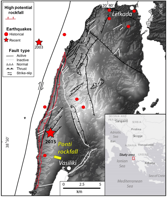
Figure 1 Map of Lefkada island, Greece, with the location of the study site (Ponti) and epicenters of recent earthquakes (stars) in 2003 (M_w = 6.2) and 2015 (M_w = 6.5), as well as historical ones (circles). The map also shows faults and high potential rockfall areas as identified by Rondoyanni et al. (2007).

On the south side of Lefkada, near the gulf of Vasiliki, a seismically triggered rockfall in Ponti village was responsible for one of the two deaths caused by the earthquake (Fig. 1). Of particular interest is the very long travel path of the rock block, which was about 800 m in plan view from the point of detachment to the end of its path. Near the end of the rockfall path, the block impacted a family residence, penetrated two brick walls and killed a person in the house. The block exited through the back of the house and came to rest in the property's backyard.

The Ponti village rockfall site is a characteristic example of how seismically induced rockfalls impact human activities. It also provides an opportunity to evaluate 2-D and 3-D rockfall analysis to predict details of the rockfall trajectory, based on field evidence. In order to create a highly accurate model of the rockfall propagation in 2-D and 3-D space, the rock path and the impact points on the slope were identified by a field survey. The study was performed using an unmanned aerial vehicle (UAV) with an ultrahigh definition (UHD) camera, which produced a high-resolution orthophoto and a digital terrain model (DTM) of the slope. The orthophoto was used to identify the rolling section and the impact points of the rock along its trajectory, which were verified by field observation. The high-resolution DTM made it possible to conduct kinematic rebound analysis and a 3-D rockfall analysis.

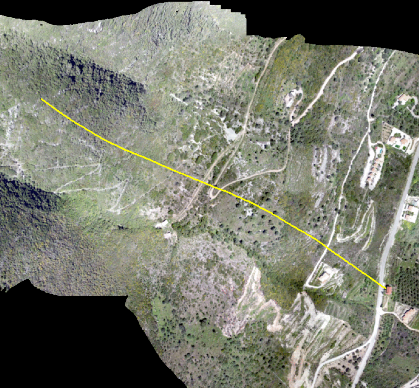
Figure 2 Orthophoto of case study. The total length of the trajectory shown with a yellow line is 800 m.

2 Ponti rockfall – site conditions

The locations of the epicenters of the 2003 and 2015 events, as well as the location of the rockfall case study, are shown in Fig. 1. The southwest coast of Lefkada is part of the Triassic to Eocene age Paxos zone and consists of limestones and dolomites that are covered by Neogene clastic sedimentary rocks, mostly sandstones and marls. Figure 1 also shows faults and high-rockfall-hazard areas as identified by Rondoyanni et al. (2007). The rockfall at Ponti is not located in an identified high-rockfall-hazard area. Based on measurements conducted at one location along the rockfall path using the multichannel analysis of surface waves method, the in situ shear wave velocity of the top layer was estimated to be around 800 m s⁻¹, which is a high velocity value and is consistent with the limestone rock at the site.

The slope overhanging Ponti village (shown in Fig. 2) has a maximum height of 600 m and an average slope angle of 35 to 40^∘. The geological formations at the Ponti rockfall site are limestones covered by moderately cemented talus materials. The thickness of the talus materials, when present, ranges between 0.5 and 4.0 m. Several detached limestone blocks were identified on the scree slope, with volumes between 0.5 and 2 m³. Based on the size distribution of these rocks on the slope, the average expected block volume would be on the order of 1 to 2 m³.

The rockfall release area was at an elevation of 500 m, while the impacted house (shown in Fig. 3) was at an elevation of 130 m. The volume of the detached limestone block was approximately 2 m³ and its dimensions were equal to 1.4 m × 1.4 m × 1 m. There was no previously reported rockfall incident at Ponti that impacted the road or a house.

3 UAV mapping

3.1 Introduction

A quadrotor UAV (Phantom 3 Professional) was deployed to reach the uphill terrain that was practically inaccessible. The UAV was equipped with an ultrahigh definition camera mentioned earlier and had the capacity to collect 4K video. The sensor was a 1/2.3^′′ CMOS (6.47 × 3.41 mm) and the effective pixel resolution was 12.4 MP (4096 × 2160 pixels). An immediate UAV data acquisition expedition was conducted 2 days after the earthquake. A second more detailed mapping UAV expedition with the objective to create a DTM was conducted 5 months after the rockfall event.

The first objective of the UAV deployment was to find the initiation point of the rock and then identify the rockfall path (shown in Fig. 2). A particular focus on that part of the task was the identification of rolling and bouncing sections of the rockfall path. In addition, to generate a high-resolution orthophoto of the rockfall trajectory, aerial video imagery was collected, and the resulting digital surface model (DSM) and digital terrain model were used to perform rockfall analysis.

The aerial survey was conducted by capturing 4K video along a gridded pattern covering the area of interest at a mean flight altitude of 115 m above the terrain resulting in image frames of a mean ground sampling distance of 4.97 cm pixel⁻¹. The minimum overlap between image frames was 80 % along the flight path and 65 % between two parallel flight paths. A total of 714 camera stations (video frames extracted) were included as shown in Fig. 4.

The structure-from-motion (SfM) methodology was implemented to create a 3-D point cloud of the terrain and develop a 3-D model. The methodology is based on identifying matching features in multiple images, and thus imagery overlap of at least 70 % is required. Compared to classic photogrammetry methodologies, where the location of the observing point is well established, SfM tracks specific discernible features in multiple images and, through nonlinear least-squares minimization (Westoby et al., 2012), iteratively estimates both camera positions, as well as object coordinates in an arbitrary 3-D coordinate system. In this process, sparse bundle adjustment (Snavely et al., 2008) is implemented to transform measured image coordinates to three-dimensional points of the area of interest. The outcome of this process is a sparse 3-D point cloud in the same local 3-D coordinate system (Micheletti et al., 2015). Subsequently, through an incremental 3-D scene reconstruction, the 3-D point cloud is densified. Paired with GPS measurements of a number of control points (for this site, 10 fast-static GPS points were collected) at the top, middle and bottom of the surveyed area, the 3-D point cloud is georeferenced to a specific coordinate system, and, through the post-processing of a digital surface model, a digital terrain model and orthophotos are created. The SfM methodology was implemented in this study using the Agisoft PhotoScan software. Precalibrated camera parameters by the SfM software (PhotoScan) were introduced and then optimized during the matching process and the initialization of ground control points (GCPs).

Figure 3 Damage from the falling rock on the impacted house in Ponti, Lefkada, Greece.

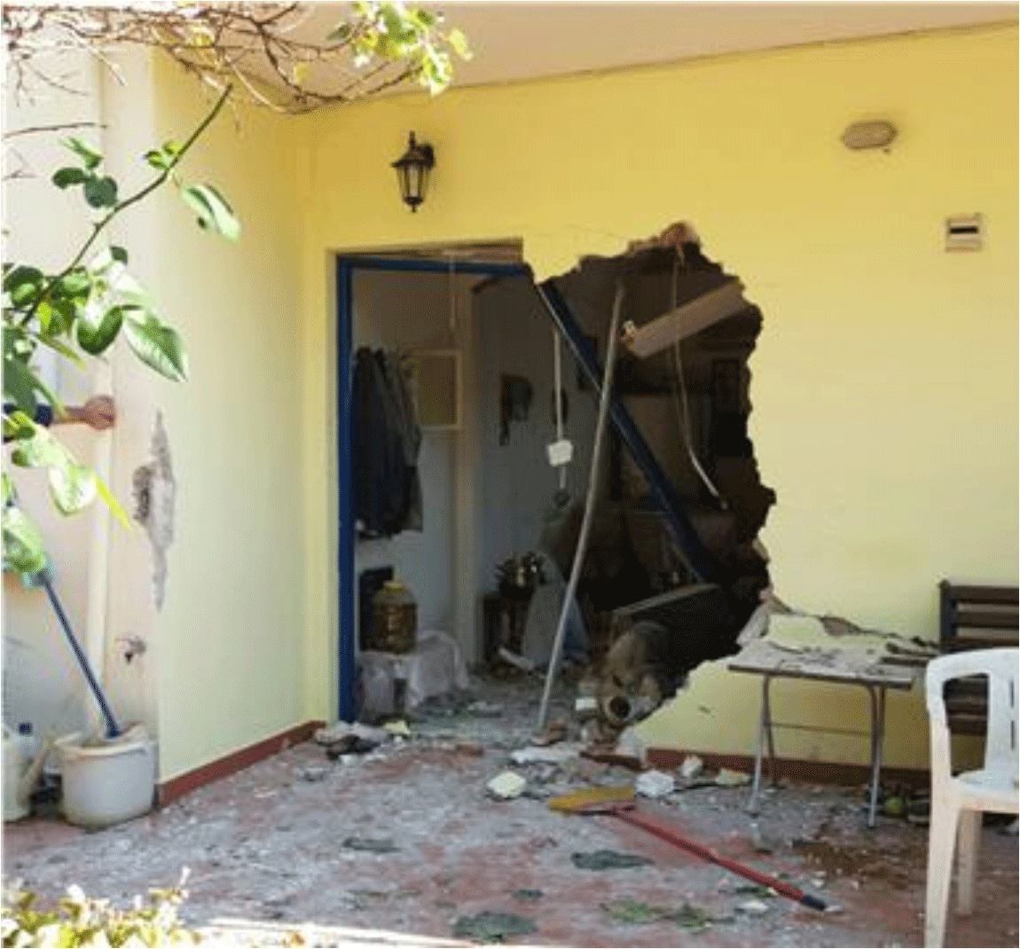
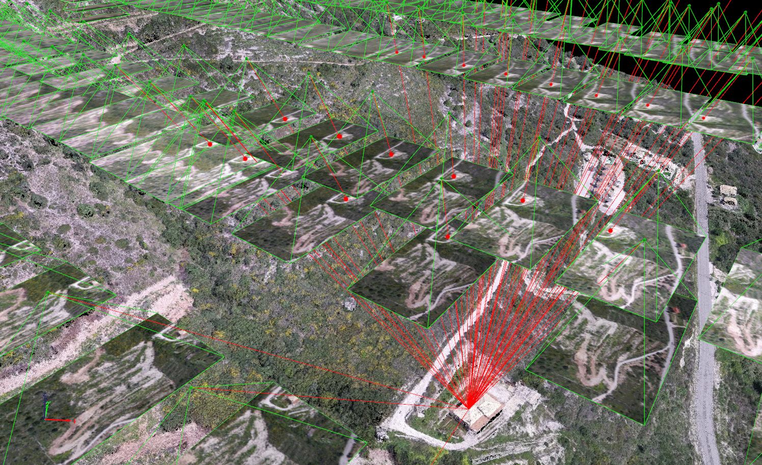
Figure 4 Schematic illustrating the overlap between pictures in the study site using SfM methodology.

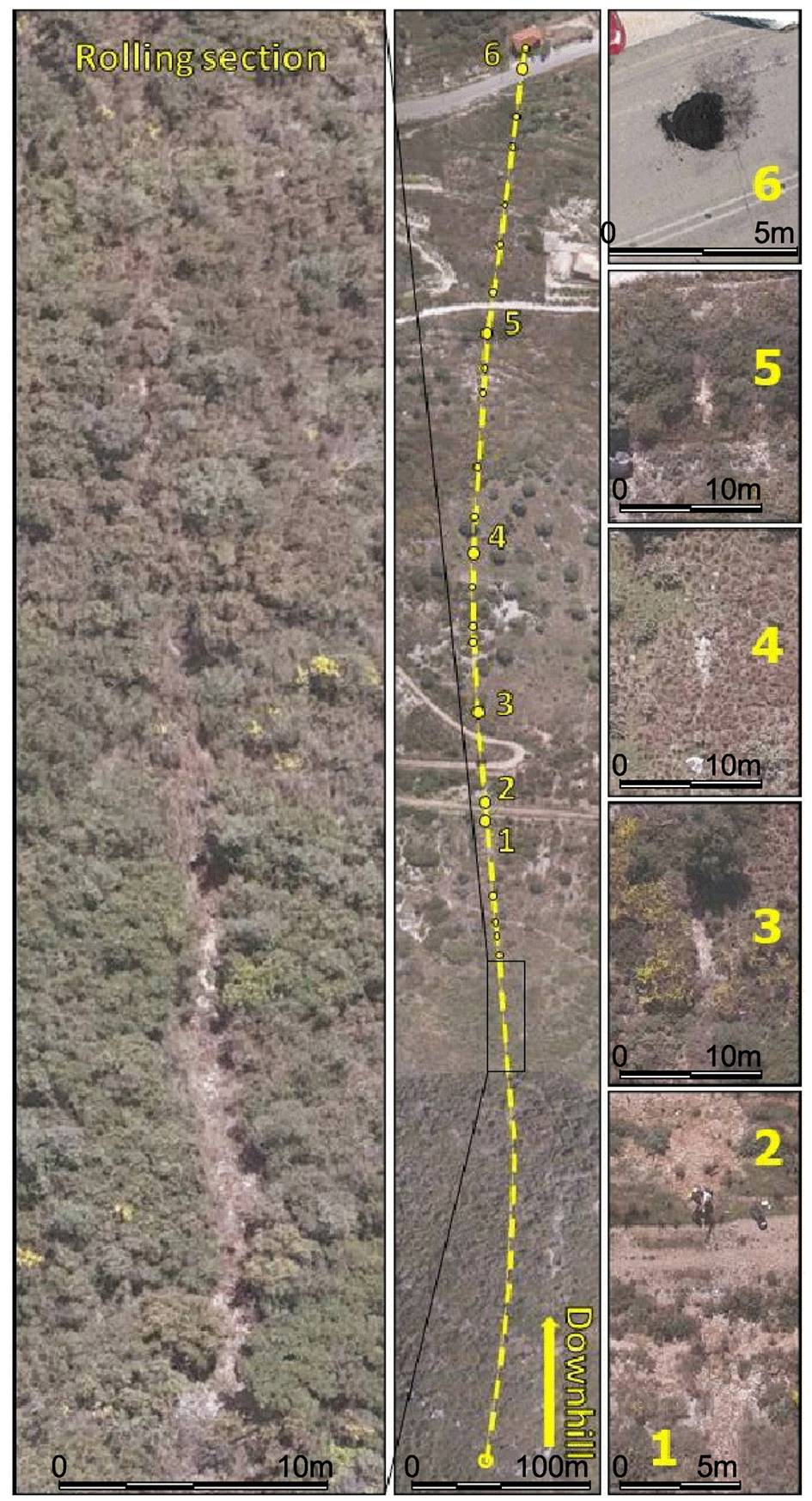
Figure 5 Top view orthophoto denoting rolling section, bouncing positions and indicative closeups of impact points.

In addition, the accuracy of the model has been examined by using portions of the ground control points and developing DTMs of differencing between different models, an investigation that is described by Manousakis et al. (2016). Finally, a comparison was made of the DTM developed by the UAV against the satellite-based DTM used for the Greek cadastre. The two surfaces were found to be very similar, as discussed subsequently.

3.2 High-resolution orthophoto

A 5 cm pixel size orthophoto was generated based on the methodology outlined earlier. As shown in Fig. 5, the rolling section and the bouncing locations of the rock block throughout its course were identified. The rolling section was easily discerned as a continuous and largely linear mark left in the vegetated terrain. Impact points that are part of the bouncing section of the rock were identified as circular to ellipsoidal bare-Earth craters with no disturbance in between. The last bouncing point before impacting the house is clearly identified on the paved road. The plan view ortho-imagery, along with the original footage of the video collected, was crucial to the qualitative identification of these features. The alternative, i.e., land-based, conventional field reconnaissance was physically impossible to perform throughout the vegetated and steep terrain.

3.3 Digital surface model and digital terrain model

A profile section and a 10 cm digital surface model were then developed (Manousakis et al., 2016), allowing the identification of features such as structures, slope benches or high trees, which could affect the rock's path downhill. Subsequently, this resolution of the DSM proved to be not only unnecessarily high and thus difficult to manipulate in subsequent rockfall analyses, but also caused numerical instabilities in the rockfall analyses. Therefore, a downscaled 2 m DTM was produced for the rockfall analysis as described next. This was implemented through the use of an aggregate generalization scheme where each output cell is assigned the minimum elevation of the input cells that are encompassed by that cell. In addition, noise filtering and smoothing processing were implemented to reduce the effect of vegetation in the final rasterized model. Note that this resolution is still higher than the resolution of DTMs that are often used in rockfall analyses.

To create the DTM, algorithms for vegetation removal were executed using the Whitebox Geospatial Analysis Tools (GAT) platform (Lindsay, 2016). The process involves point cloud neighborhood examination and digital elevation model (DEM) smoothing algorithms. Firstly, a bare-Earth DEM was interpolated from the input point cloud LAS file, by specifying the grid resolution (2 m) and the inter-point slope threshold. The algorithm distinguished ground points from non-ground points based on the inter-point slope threshold. Thus, the interpolation area was divided into lattice cells, corresponding to the grid of the output DEM. All of the point cloud points within the circle containing each grid cell were then examined as a neighborhood. Those points within a neighborhood that have an inter-point slope with any other point and are also situated above the corresponding point are attributed as non-ground points. An appropriate value for the inter-point slope threshold parameter depends on the steepness of the terrain, but generally values of 15–35^∘ produce satisfactory results. The elevation assigned to the grid cell was then the nearest ground point elevation (Lindsay, 2016).

Further processing of the interpolated bare-Earth DEM was executed to improve vegetation and structures' removal results by applying a second algorithm to point cloud DEMs, which frequently contain numerous off-terrain objects (OTOs) such as buildings, trees and other vegetation, cars, fences and other anthropogenic objects. The algorithm works by locating and removing steep-sided peaks within the DEM. All peaks within a subgrid, with a dimension of the user-specified OTO size, in pixels, were identified and removed. Each of the edge cells of the peaks were then queried to check if they had a slope that is less than the user-specified minimum OTO edge slope and a back-filling procedure was used. This ensures that natural topographic features such as hills are not recognized and confused as off-terrain features (Whitebox GAT help topics).

The final DTM model had a total RMS error after filtering for six GCPs that was 0.07 m, while the total RMS error for four checkpoints was 0.20 m. When compared to a 5 m DEM from the Greek National Cadastre with a geometric accuracy of RMSEz ≤ 2.00 m and absolute accuracy ≤ 3.92 m for a confidence level of 95 %, a mean difference of 0.77 m and a standard deviation of 1.25 m is observed, which is well into the range of uncertainty of the cadastre model itself.

4 Earthquake characteristics – initial conditions

4.1 Seismic acceleration

The epicenter of the earthquake according to the National Observatory of Athens Institute of Geodynamics (NOA) is located onshore near the west coast of Lefkada. The causative fault is estimated to be a near-vertical strike-slip fault with dextral sense of motion (Ganas et al., 2015, 2016). Based on the focal mechanism study of the earthquake, it was determined that the earthquake was related to the right lateral Kefalonia–Lefkada Transform Fault, which runs nearly parallel to the west coasts of both Lefkada and Kefalonia island, in two segments (Papazachos et al., 1998; Rondoyanni et al., 2007).

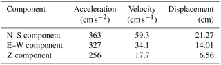
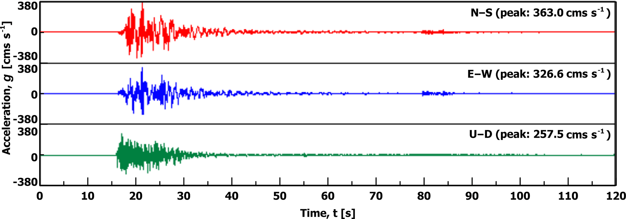
A strong motion station recorded the ground motions in the village of Vasiliki located at a distance of 2.5 km from the Ponti rockfall site. The ground motion characteristics of the recording are summarized in Table 1 and are presented in Fig. 6 (ITSAK, 2016).

Table 1 Accelerometer recordings.

Figure 6 Acceleration time history recording at the Vasiliki site (ITSAK, 2016).

4.2 Topography effect

Peak ground acceleration along the rock slope is estimated from the PGA of the base (PGA_b) modified by site and topographic effects (Mavrouli et al., 2009). In the present case, local shaking intensity in terms of horizontal PGA was considered. The E–W component of acceleration was considered for the determination of the initial velocity. The peak ground acceleration on the slope face (PGA_sf) was considered equal to the acceleration at the slope crest (PGA_cr). The acceleration at the base was equal to 0.32 g and thus at the crest PGA_cr = 1.5 PGA_b was equal to 0.48 g.

4.3 Initial velocity of the rock block

The initial horizontal velocity of the block, at the time of detachment, was calculated considering equilibrium of the produced work and the kinetic energy according to Eq. (1).

$$\begin{array}{}\text{(1)}& {\displaystyle }{\displaystyle }{v}_x=\sqrt{\mathrm{2}\times {\mathrm{PGA}}_{\mathrm{sf}}\times s},\end{array}$$

where PGA_sf is the acceleration on the slope at the location of detachment and s the initial displacement of the block in order to initiate its downslope movement.

The initial horizontal velocity was calculated equal to 0.67 m s⁻¹, considering a displacement on the order of s = 0.05 m. The vertical component of the initial velocity is assumed to be zero.

5 Trajectory analysis

In order to estimate the possible rock paths and design remedial measures, simulation programs based on lumped-mass analysis models are commonly used in engineering practice. The trajectory of a block is modeled as a combination of four motion types: free falling, bouncing, rolling and sliding (Descoeudres and Zimmermann, 1987). Usage of the lump-mass model has some key limitations – the block is described as rigid and dimensionless, with an idealized shape (sphere); therefore, the model neglects the block's actual shape and configuration at impact, even though both affect the resulting motion.

5.1 Modeling the response to an impact

The most critical input parameters are the coefficients of restitution (CORs), which control the bouncing of the block. In general, the coefficient of restitution is defined as the decimal fractional value representing the ratio of velocities (or impulses or energies, depending on the definition used) before and after an impact of two colliding entities (or a body and a rigid surface). When in contact with the slope, the block's magnitude of velocity changes according to the COR value. Hence, COR is assumed to be an overall value that takes into account all the characteristics of the impact, including deformation, sliding upon contact point and transformation of rotational moments into translational moments and vice versa (Giani, 1992).

The most widely used definitions originate from the theory of inelastic collision as described by Newtonian mechanics. For an object impacting a rocky slope (Fig. 7), which is considered as a steadfast object, the kinematic COR (v_COR) is defined according to Eq. (2):

$$\begin{array}{}\text{(2)}& {\displaystyle }{\displaystyle }{v}_{\mathrm{COR}}={\displaystyle \frac{v_{\mathrm{r}}}{v_{\mathrm{i}}}},\end{array}$$

where v is the velocity magnitude and the subscripts “i” and “r” denote the trajectory stage – incident (before impact) and rebound (after impact) respectively.

Figure 7 Coefficients of restitution.

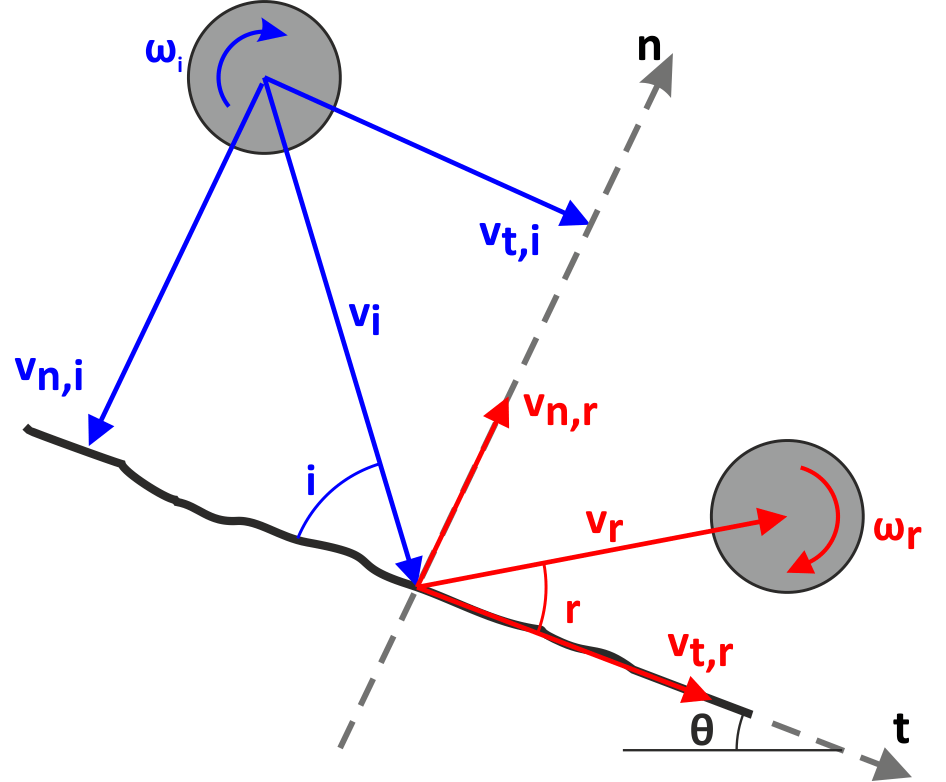
Two different mechanisms participate in the energy dissipation process; energy loss normal to the slope is attributed to the deformation of the colliding entities and loss in the tangential direction is due to friction between them. Therefore kinematic COR has been analyzed for the normal and tangential component with respect to the slope surface, defining the normal (n_COR) and the tangential (t_COR) coefficients of restitution (Eqs. 3 and 4 respectively):

$$\begin{array}{}\text{(3)}& {\displaystyle }{\displaystyle }{n}_{\mathrm{COR}}={\displaystyle \frac{v_{\mathrm{n},\mathrm{r}}}{v_{\mathrm{n},\mathrm{i}}}}\end{array}$$

and

$$\begin{array}{}\text{(4)}& {\displaystyle }{\displaystyle }{t}_{\mathrm{COR}}={\displaystyle \frac{v_{\mathrm{t},\mathrm{r}}}{v_{\mathrm{t},\mathrm{i}}}},\end{array}$$

where the first subscript, “n” or “t” denotes the normal or the tangential components of the velocity respectively.

Normal and tangential CORs have prevailed in natural hazard mitigation design via computer simulation due to their simplicity. Values for the coefficients of restitution are acquired from values recommended in the literature (e.g., Azzoni and de Freitas, 1995; Heidenreich, 2004; Richards et al., 2001; RocScience, 2004). These values are mainly related to the surface material type and originate from experience, experimental studies or back analysis of previous rockfall events. This erroneously implies that coefficients of restitution are material properties. However, COR values depend on several parameters that cannot be easily assessed. Moreover, values suggested in the literature vary considerably and are sometimes contradictory.

5.2 Rockfall path characteristics

A total of 23 impact points were identified on the slope surface (Fig. 8). Their coordinates are presented in Table 2, along the block's path starting from the detachment point (where x = 0). No trees were observed along the block's path.

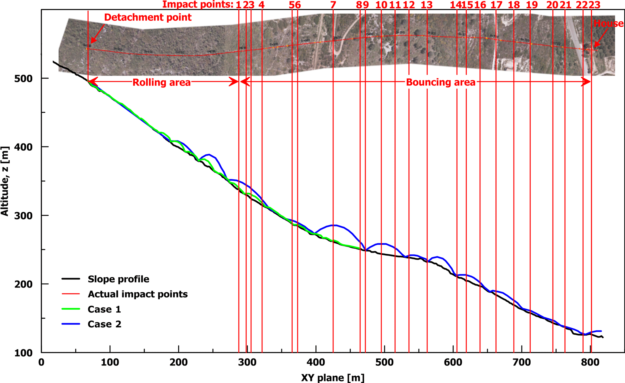
Figure 8 Plan view and cross section along the block's path (units in m); 2-D rockfall trajectory analysis results are plotted with the green and blue line.

Figure 9 Out-of-plane geometry.

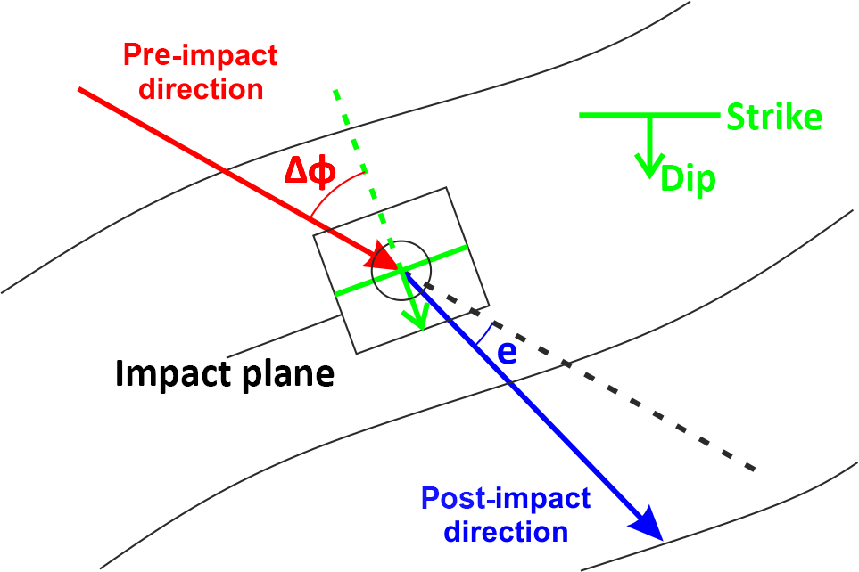
The apparent dip of the slope at impact positions was measured from the DTM; on each impact point a line was set with a length twice the block's mean dimension, oriented according to preceding trajectory direction. Moreover, the impact point was expanded on the DTM to a rectangular plane with a side twice the mean dimension of the block (Fig. 9). This plane was then oriented so that one side coincides with the strike direction and its vertical side towards the dip direction. Thus, direction difference, Δφ, was measured by strike direction and the preceding path and deviation, e, was measured as the angle between pre- and post-impact planes (Asteriou and Tsiambaos, 2016).

Having a detailed field survey of the trajectory path, a back analysis according to the fundamental kinematic principles was performed with the intent to back-calculate the actual COR values.

5.3 Kinematic analysis and assumptions

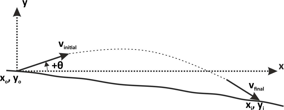
The 23 impact points identified on the slope comprise a rockfall path of 22 parabolic segments. The vertical and horizontal length of each segment is acquired by subtracting consecutive points. Since no external forces act while the block is in midair, each segment lays on a vertical plane and is described by the general equation of motion as

$$\begin{array}{}\text{(5)}& {\displaystyle }{\displaystyle }y=x\tan \mathit{\theta }-{\displaystyle \frac{g{x}^{\mathrm{2}}}{\mathrm{2}{v}_{\mathrm{i}}^{\mathrm{2}}{\cos }^{\mathrm{2}}\mathit{\theta }}},\end{array}$$

where θ is the launch angle from the horizon and v is the launch (initial) velocity (Fig. 10).

Figure 10 Parabolic segment.

Since no evidence can be collected regarding launch angle and velocity, innumerable parabolas satisfy Eq. (5). However, θ is bound between −β and 90^∘, so, in order to acquire realistic values for the initial velocity, its sensitivity for that range was investigated.

For the case presented in Fig. 11 (the first parabolic segment) it is shown that for the majority of the release angles, initial velocity variation is low and ranges between 7.2 and 12 ms⁻¹. Additionally, the relationship between release angle and initial velocity is expressed by a curvilinear function, with a minimum initial velocity value along with an associated release angle (denoted hereafter as θ_cr).

Given the minimum initial velocity and the critical release angle for each parabolic segment, the impact velocity and impact angle can be calculated. Subsequently, normal and tangential velocity components according to the apparent dip of the impact area are calculated in order to evaluate COR values. Results are summarized in Table 3.

5.4 Coefficients of restitution

It is observed that v_cor (Table 3) is greater than 1 in 5 out of 22 impacts. According to Eq. (3), this can only be achieved when impact velocity is less than rebound velocity. However, this indicates that energy was added to the block upon impact, which is not possible according to the law of conservation of energy. Thus, impact velocity should be greater, which is possible if the launch velocity of the previous impact was higher than the assumed minimum.

For the cases where V_cor < 1, it is observed that kinematic COR ranges between 0.55 and 1.0 and presents smaller variation compared to the normal or tangential coefficient of restitution, similar to what was previously reported in the relevant literature (i.e., Asteriou et al., 2012; Asteriou and Tsiambaos, 2016).

Table 2 Impact points characteristics.

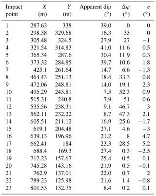
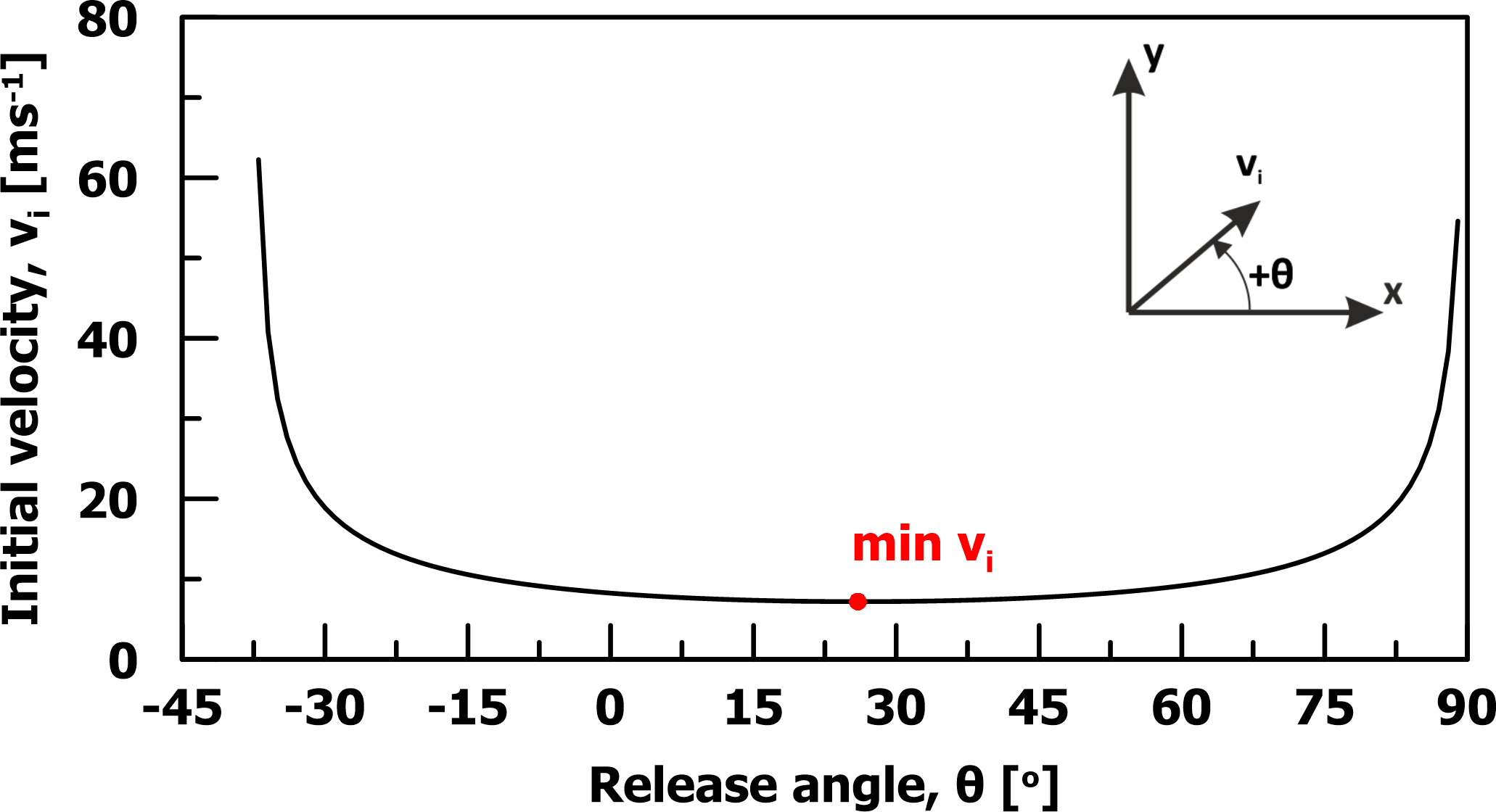
Figure 11 Release angle versus initial velocity for the first parabolic section (δx = 10.75 m, δy = 8.33 m).

Figure 12 Normal COR versus impact angle.

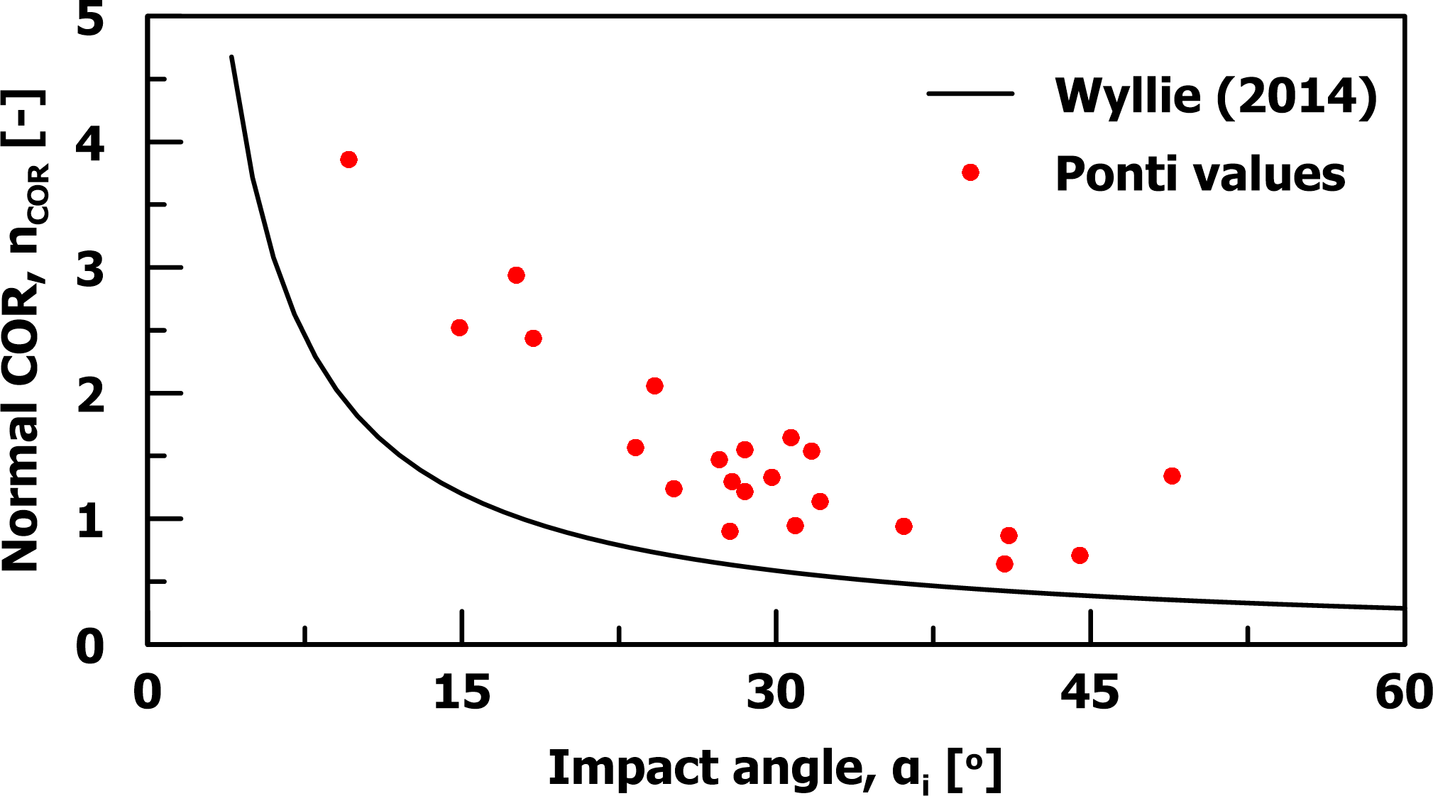
The wide scatter of the normal COR implies that the restitution coefficient cannot be a material constant. Yet, in most relevant software, the normal COR is defined solely by the slope material. Moreover, normal COR values higher than one were calculated in 11 out of the 15 remaining impacts. Normal CORs higher than one have been observed in both experimental (e.g., Spadari et al., 2011; Buzzi et al., 2012; Asteriou et al., 2012) and back-analysis studies (e.g., Paronuzzi, 2009) and are related to irregular block shape and slope roughness, as well as to shallow impact angle and angular motion. A more detailed presentation of the reasons why the normal COR exceeds unity can be found in Ferrari et al. (2013). However, in rockfall software used in engineering practice, normal COR values are bounded between 0 and 1.

As shown in Fig. 12, the normal COR increases as the impact angle reduces, similarly to previous observations by Giacomini et al. (2012), Asteriou et al. (2012) and Wyllie (2014). The correlation proposed by Wyllie (2014) is also plotted in Fig. 13 and seems to describe consistently, but on the nonconservative side, the trend and the values acquired by the aforementioned analysis and assumptions.

Table 3 Parabolic paths characteristics for the minimum release velocity.

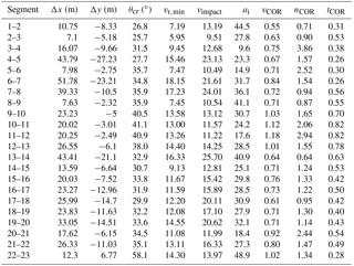
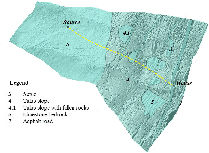
Figure 13 Soil types for 3-D rockfall analysis (according to Rockyfor3D). The yellow line showing the path of the trajectory is 800 m.

6 Rockfall modeling

6.1 Two-dimensional analyses

A deterministic 2-D rockfall analysis was first performed using RocFall software (RocScience, 2004). According to Asteriou and Tsiambaos (2016) the most important influence is posed by the impact configuration, which is influenced by slope roughness and block shape. In this study, roughness has been fully taken into account (considering the block's dimension scale) by the high resolution of the cross section used in the analyses (more than 1500 x–y points were used – approximately two points per meter). Based on our experience, this resolution is significantly higher compared to other rockfall studies. Moreover, it was not possible to simulate block shape effect nor the configuration of the block at impact using lumped-mass model analysis.

Considering an initial velocity of 0.67 m s⁻¹, according to the numerical analyses, the falling rock primarily rolls on the slope and stops much earlier than its actual (field-verified) runout distance, approximately 400 m downslope from its initiation point (Fig. 8; case 1). The restitution coefficients were n_COR = 0.35 and t_COR = 0.85 and were selected based on the suggested values for bedrock outcrops provided in the software documentation.

Note that for this analysis the friction angle was set to zero. A standard deviation for the coefficients of restitution, the friction angle and roughness of the material on the slope was not used for this deterministic analysis. For friction equal to 32^∘ (as suggested by the software documentation), the rock travels downslope only 50 m.

Additional analysis was also performed, with lower coefficients of restitution that are representative of the talus material on the slope (n_COR = 0.32, t_COR = 0.82, φ = 30^∘) per the software documentation. In this case, the rock block rolled only a few meters downslope. Therefore, it is evident that the actual rock trajectory cannot be simulated.

Table 4 Restitution parameters for Rockyfor3D.

In order to more closely simulate the actual trajectory, various combinations of restitution coefficients and friction angle were considered. The closest match occurred for n_COR = 0.60 and t_COR = 0.85, while the friction angle was set to zero and no velocity scaling was applied. For these input parameters, the rock block reaches the house with a velocity of approximately 18 m s⁻¹ (Fig. 8; case 2). These values for the restitution coefficients correspond to a bedrock material (limestone).

Even in this case, the modeled trajectory is significantly different from the actual one. The main difference is that the block rolls up to 200 m downslope while the actual rolling section is 400 m (as shown in Fig. 8). Furthermore the impacts on the ground in the bouncing section of the trajectory are considerably fewer in number (14 versus 23) and in different locations compared to the actual ones. Finally, the bounce height of some impacts seems unrealistically high. For example, the second bounce has a jump height (f) of ∼ 17.5 m over a length (s) of ∼ 50 m, resulting in a f∕s ratio of ∼ 1∕3 when the characteristic f∕s ratios for high, normal and shallow jumps are 1∕6, 1∕8 and 1∕12 respectively, as suggested by Volkwein et al. (2011).

6.2 Three-dimensional rockfall analysis

The rockfall trajectory model Rockyfor3D (Dorren, 2012) has also been used in order to validate the encountered trajectory and assess the probability that the falling rock (from the specific source area) reaches the impacted house.

The 3-D analysis was based on the down-scaled 2 m resolution digital terrain model that was generated from the 10 cm DSM. The following raster maps were developed for the 3-D analysis: (a) rock density of rockfall source; (b) height, width, length and shape of block; (c) slope surface roughness; and (d) soil type on the slope, which is directly linked with the normal coefficient of restitution, n_COR.

Figure 14 Reach probability graph calculated from 3-D rockfall analysis.

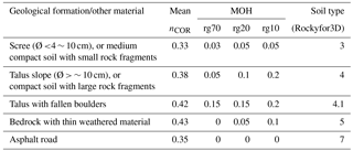
The slope roughness was modeled using the mean obstacle height (MOH), which is the typical height of an obstacle that the falling block encounters on the slope at a probability of 70, 20 and 10 % of the trajectories (according to the suggested procedure in Rockyfor3D). No vegetation was considered in the analysis, which favors a longer trajectory. The parameters considered in the 3-D analysis for the different formations are summarized in Table 4. The spatial occurrence of each soil type is shown in Fig. 13 and the assigned values of n_COR are according to the Rockyfor3D manual. The values for soil type 4.1 in Fig. 13 are slightly different from those of soil type 4 (proposed in the manual), denoting talus with a larger percentage of fallen boulders. The block dimensions were considered equal to 2 m³ and the shape of the boulder was a rectangle. In order to simulate the initial velocity of the falling rock due to the earthquake, an additional initial fall height is considered in the analysis, which for this case was set equal to 0.5 m.

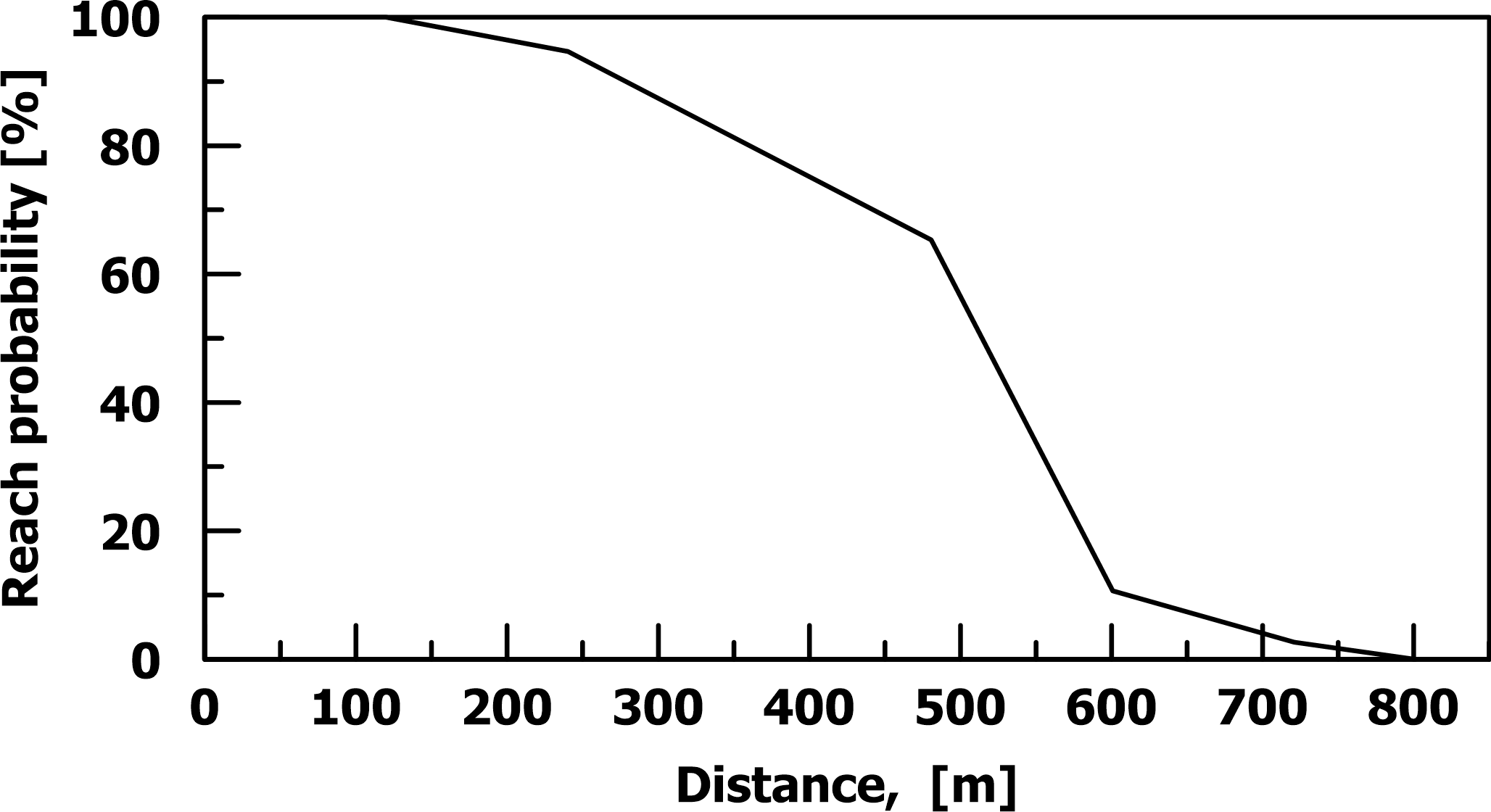
The energy line angles were recalculated from the simulated trajectories and it was determined that the energy line angle with highest frequency (39 %) was 30–31^∘. Based on the 3-D analysis no rock blocks would impact the house, although the rock paths are closer to the actual trajectories compared to RocFall software. The reach probability of the falling rocks, initiating from the source point, is shown in Fig. 14. Reach probability is the percentage of the falling rocks in relation to the total number of falling rocks that reach a specific point along the line of the trajectory.

6.3 Lateral dispersion and deviation

Lateral dispersion is defined as the ratio between the distance separating the two extreme fall paths (as seen looking at the face of the slope) and the length of the slope (Azzoni and de Freitas, 1995). According to Crosta and Agliardi (2004) the factors that control lateral dispersion are (a) macro-topography factors, which are factors related to the overall slope geometry; (b) micro-topography factors controlled by the slope local roughness; and (c) dynamic factors, which are associated with the interaction between slope features and block dynamics during bouncing and rolling. Based on an experimental investigation, Azzoni and de Freitas (1995) noted that the dispersion is generally in the range of 10 to 20 %, regardless of the length of the slope, and that steeper slopes exhibit smaller dispersion. Agliardi and Crosta (2003) calculated lateral dispersion to be up to 34 %, using high-resolution numerical models on natural rough and geometrically complex slopes.

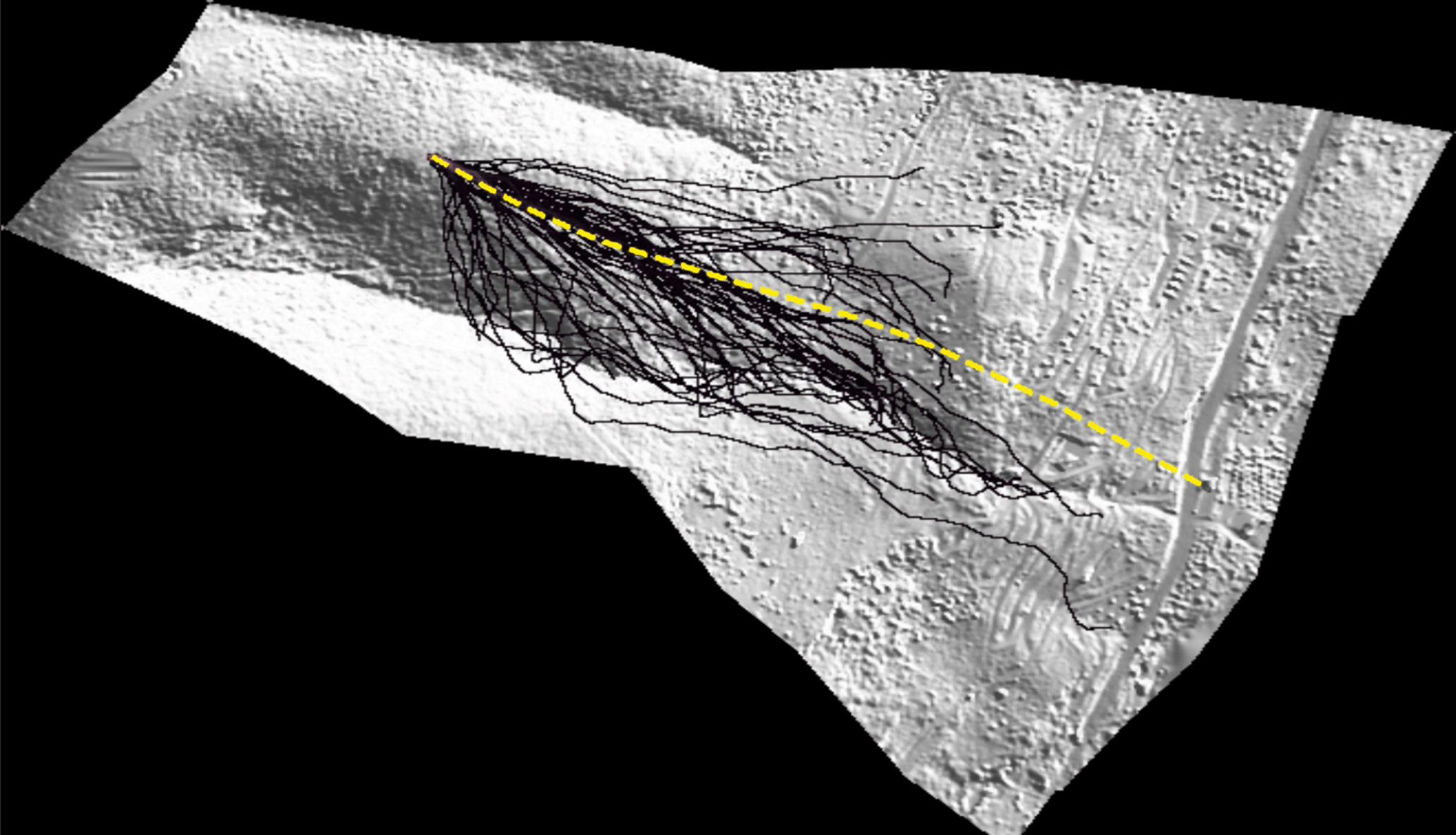
Figure 15 Three-dimensional trajectory analysis (from Rockyfor3D analysis). The yellow line shows the actual trajectory. Black lines show the simulated trajectory.

Lateral dispersion cannot be defined from the actual rockfall event in Ponti since only one path is available. Using the simulated trajectories from Rockyfor3D, which are in the 3-D space (Fig. 15), a lateral dispersion of approximately 60 % is shown in the middle of the distance between the detachment point and the house. This is significantly higher dispersion than the findings of Azzoni and de Freitas (1995) and Agliardi and Crosta (2003). The lateral dispersion computed by Rockyfor3D is extremely pronounced and most likely due to the topography effect of the area of detachment. Specifically, the origin of the rock block is located practically on the ridgeline, facilitating the deviation of the rockfall trajectory from the slope line.

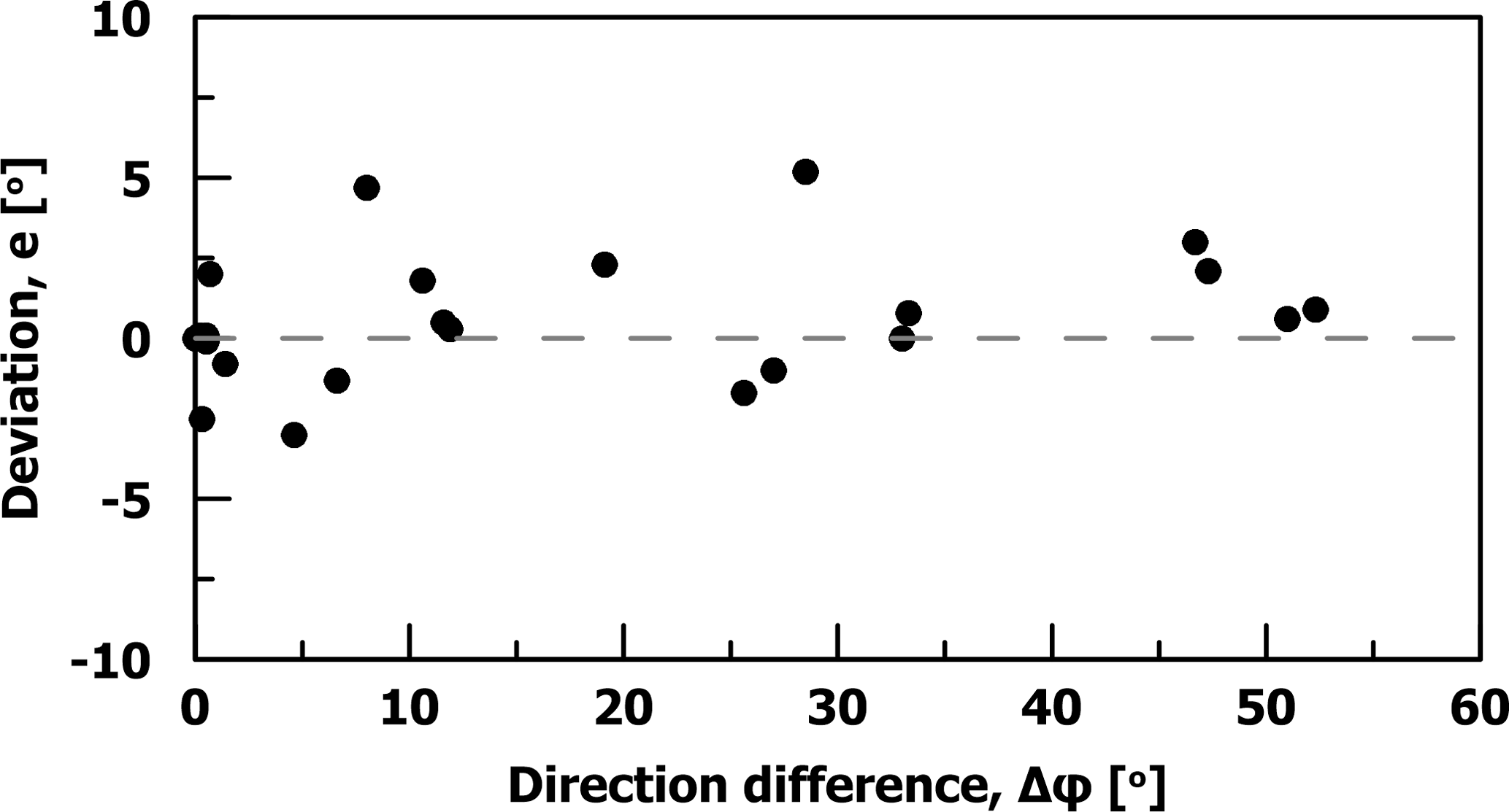
Asteriou and Tsiambaos (2016) defined deviation (e) as the dihedral angle between the pre- and post-impact planes that contain the trajectory. They found that deviation is controlled by the direction difference Δφ, the slope inclination and the shape of the block. For a parallel impact (i.e., Δφ = 0^∘), a spherical block presents significantly less deviation compared to a cubical. Additionally, deviation is equally distributed along the post-impact direction and reduces as the slope's inclination increases. On oblique impacts, the block's direction after impact changes towards the slope aspect, and as Δφ increases this trend becomes more pronounced.

Figure 16 illustrates the relationship of deviation with direction difference. It is noted that, for parallel impacts (Δφ = 0^∘), deviation is uniformly distributed along the post-impact direction. As direction difference increases, the deviation becomes positive, which means that the change in direction follows the direction of slope's aspect. These findings are consistent with trends described by Asteriou and Tsiambaos (2016), but the deviation of the actual trajectory is significantly lower. This can be attributed to the different conditions (i.e., block shape, slope material, slope roughness, incident velocity and angle, and scale) between the experimental program conducted by Asteriou and Tsiambaos (2016) and the Ponti rockfall event.

Figure 16 Deviation as a function of direction difference.

7 Conclusions

UAV-enabled reconnaissance was successfully used for the identification of the origin of the detached rock, the rockfall trajectory and the impact points on the slope, and especially for discerning the rolling and bouncing sections of the trajectory. A UAV with an ultrahigh definition camera was deployed to reach the inaccessible, steep and partly vegetated uphill terrain. A high-resolution orthophoto of the rockfall trajectory, a 10 cm DSM and a 2 m DTM were generated and formed the basis for an analytical 2-D kinematic analysis and a comparison with the outcomes of 2-D and 3-D rockfall analysis software.

The findings from this study indicate that UAV-based photogrammetry can be a low-cost alternative to lidar surveying for developing DTMs. Acquisition of a UAV with a high-resolution camera is significantly less expensive than the acquisition cost of a lidar or a total laser scanner unit that generates similar (i.e., point cloud) data. In addition, deployment of UAVs is simpler and less expensive. Among the many advantages of UAV-enabled SfM is the ability to access areas that are relatively inaccessible. This advantage is particularly important in emergency response and reconnaissance following natural disasters such as landslides, floods, earthquakes and hurricanes.

However, experience is necessary to generate data of appropriate quality (spatial distribution and resolution), as data quality is significantly affected by the sensor data as well as the flight characteristics. Ground control points are critical to properly scale the point clouds and reduce distortions.

The initial velocity of the detached rock was estimated based on site conditions and amplification of the ground acceleration due to topography. It was found that the initial velocity of the blocks plays a significant role in the accurate reproduction of the rockfall trajectory.

Based on the computational analysis performed, it was found that the coefficients of restitution cannot be directly connected to the material type, nor can they be considered material constants. The impact angle seems to influence the normal COR, which has been also observed in other recent studies but has not been incorporated yet on analysis models.

It was proven impossible to replicate the actual trajectory of the rockfall by performing a 2-D rockfall analysis with the recommended set of parameters indicating limitations in the present formulations. In an attempt to match the actual rock path to the analysis output, the friction angle of the limestone slope was considered equal to zero. However, the falling rock still rolled on the slope and stopped much earlier than its actual runout distance while the impacts on the ground in the bouncing section of the trajectory were considerably different in number and in location compared to the actual ones.

Using the 3-D analysis software and recommended input parameters, rock trajectories better approximated the actual trajectory, indicating that the 3-D analysis can be more accurate than the 2-D analysis.

Based on the aforementioned analyses it becomes evident that engineering judgement and experience must accompany the usage of rockfall software in order to acquire realistic paths. The recommended set of parameters should be used with caution since field performance can differ significantly, as demonstrated by this case study.