Tree-based mesh-refinement GPU-accelerated tsunami simulator for real-time operation

This paper presents a fast and accurate tsunami real-time operational model to compute across ocean-wide simulations completely on GPU (graphics processing unit). The spherical shallow water equations are solved using the method of characteristics and upwind cubic interpolation to provide high accuracy and stability. A customized, user interactive, tree-based mesh-refinement method is implemented based on distance from the coast and focal areas to generate a memory-efficient domain with resolutions of up to 50 m. Three specialized and optimized GPU kernels (Wet, Wall and Inundation) are developed to compute the domain block mesh. Multi-GPU is used to further speed up the computation, and a weighted Hilbert space-filling curve is used to produce a balanced workload. Hindcasting of the 2004 Indonesian tsunami is presented to validate and compare the agreement of the arrival times and main peaks at several gauges. Inundation maps are also produced for Kamala and Hambantota to validate the accuracy of our model. Test runs on three Tesla P100 cards on Tsubame 3.0 could fully simulate 10 h in just under 10 min wall-clock time.

1 Introduction

The turn of the 21st century showed us, as never before, the reality of the terrible and devastating damage and death that tsunamis can cause. In 2004, a massive earthquake off Sumatra Island of magnitude M_w=9.0 on the Richter scale triggered a tsunami with deadly consequences. According to the World Health Organization, the death toll for these events exceeds 200 000 (WHO, 2014) in several countries spread along the Indian Ocean. Not much later in 2011, a tsunami triggered by a M_w=9.0 earthquake on the east coast of Japan in the Tohoku region produced yet another disaster. Over 15 000 people died from these events, with massive destruction of port and city infrastructure, housing, and telecommunications. Additionally, the subsequent nuclear crisis was due to the tsunami-induced damage of several reactors in the Fukushima nuclear power plant (Motoki and Toshihiro, 2012).

These events highlight the importance of developing accurate and fast tsunami-forecasting models. For several decades, efforts have been made to develop such models. These can be classified into two main groups: depth-average (i) hydrostatic and (ii) non-hydrostatic long wave equations. Hydrostatic models for the shallow water equations (SWEs) started by solving their linear form based on finite difference methods (FDMs), following the work of Hansen (1956) and Fischer (1959) in the 1950s. The TUNAMI (Tohoku University's Numerical Analysis Model for Investigation) (Imamura et al., 1995) came from these initial steps but solved the shallow water equations in a nonlinear form instead, formulated them in a flux-conservative way for mass conservation and also introduced a discharge computation (Imamura, 1996) for the elevation near the shoreline. In a very similar manner, the ALASKA-tectonic (GI'-T) and Landslide models (GI'-L) were introduced, which solved the nonlinear shallow water and used leapfrog FDM (Nicolsky et al., 2011) similar to TUNAMI. Later came MOST (Method of Splitting Tsunami) (Titov and Synolakis, 1995), an extensively used model for tsunami simulation that tried to incorporate the effect of dispersion during simulations (Burwell et al., 2007). It was original because it introduced a function to add points in the shoreline to improve tracking. Recently, MOST has been ported for GPU computing (Vazhenin et al., 2013). A more recent model is GeoClaw, which implements a unique approach to deal with the issue of transferring fluid kinematics throughout nested grids by refining specified cells during simulation to improve resolution in those areas (Berger and LeVeque, 1998). More recent models incorporate a real-time application such as RIFT (Real-Time Inundation Forecasting of Tsunamis) (Wang et al., 2012). Like several of the previous models, a leapfrog scheme is also used for these real-time models, and a linear SWE is solved in certain areas for lighter computation. COMCOT (Cornell Multi-grid Coupled Tsunami Model) from Cornell University is another example using this approach (Liu, 1998). EasyWave is another model (Babeyko, 2017) which employs linear approximations to improve speed and employs a leapfrog scheme as its numerical scheme. The latest version of EasyWave introduced GPU to accelerate parts of the existing CPU code. More recently, GPU-based models have been developed, like NAMI DANCE (Zaytsev et al., 2006) in its latest version. Additionally, a better known GPU model, Tsunami-HySEA (Macías et al., 2017), has been extensively tested and is currently used by the Centro di Allerta Tsunami (CAT) in Italy.

In order to include the effect of pressure, since the 1990s, some models have taken the direction of solving non-hydrostatic models using the depth-integrated Boussinesq equations (BEs) instead of the SWEs for tsunami propagation. Initial efforts considered them to be weak nonlinear models (Peregrine, 1967); however, models for nonlinear equations were also developed not long after (for instance, Nwogu, 1993; Lynett et al., 2002). Solving the Boussinesq equation is, in general, more computationally demanding than solving the SWEs and in order to reduce the computational time, some techniques have been implemented, such as using parallel clusters or introducing nested grids. An example of this is FUNWAVE-TVD (Shi et al., 2012), which is an extended version of FUNWAVE, a run-up and propagation model based on fully nonlinear and dispersive Boussinesq equations (Wei et al., 1995). FUNWAVE introduced a nested-grid method, and its later version was fully parallelized using MPI-FORTRAN. A well-known non-hydrostatic model which also implements two-way grid nesting is NEOWAVE (Non-hydrostatic Evolution of Ocean WAVE; Yamazaki et al., 2011). Another one of these models is BOSZ (Roeber and Cheung, 2012), which combines the dispersive effect from the BEs with the shock-capturing ability of the nonlinear SWEs. BOSZ is mainly used for nearshore simulation, since it is based on Cartesian coordinates and not suited for large areas. Additionally, it does not implement nested grids.

Recently, efforts to solve the modeling equations in three dimensions have been made as well. Although these models tend to capture difficult coastlines very well and can include multiple fluids or even materials, the computation cost is still so great that it makes it only possible to apply them effectively in small areas and it is not viable for transoceanic propagations. Some examples are SELFEs (semi-implicit Eulerian–Lagrangian finite elements; Zhang and Baptista, 2008; Abadie et al., 2010, 2012; Horrillo et al., 2013).

In this work, we present a new approach for a tsunami operational model that retains a high degree of the complexities of the physics involved and delivers a fast and accurate simulation. This speed also enables real-time operation: a user can start forecasting simultaneously as a tsunami event occurs. Results are generated faster than real time. The main goal is to accomplish a wide-area, ocean-size computation in short time while using resources efficiently. Our model, referred to hereinafter as TRITON-G (Tsunami Refinement and Inundation Real-Time Operational Numerical Model for GPU), implements a full-GPU computing approach for the whole tsunami model, composed of generation, propagation and inundation. Specialized kernels are developed for each part of the tsunami computation, and multi-GPU is used for further acceleration. Load balance is obtained using a weighted Hilbert space-filling curve. TRITON-G solves the nonlinear spherical shallow water equations across the entire domain to preserve the complexity of the propagation and the effects near the coastline. The method of characteristics with directional splitting and a third-order interpolation semi-Lagrangian numerical scheme is used to solve the governing equations. This allows for high accuracy and minimizes effects of numerical dispersion and diffusion while also giving the ability to choose a larger time step compared to using a Runge–Kutta scheme and at the same time permits a light stencil suitable for fast computation. We implement a tree-based block refinement to generate a computational mesh that is flexible, light and can track complex coastlines. Customized refinements by distance and focal area were developed, which permitting an efficient use of memory and computational resources. In a collaborative project with RIMES (Regional Integrated Multi-Hazard Early Warning System, 2017), we utilize their existing databases for bathymetry and fault sources where available and successfully deployed TRITON-G as their tsunami forecast operational model.

This article is organized as follows. A review of the governing equations is given in Sect. 2. The numerical method and boundaries are explained in Sect. 3. In Sect. 4, a description of tree-based refinement and its customization is given. The topography and bathymetry used are also described. GPU and parallel computing are covered in Sect. 5. In Sect. 6, we present comparison results with a known benchmark inundation problem. In Sect. 7, we present several numerical results including TRITON-G validation with existing tsunami propagation data and run-up measurements. Section 8 presents the conclusions of this study. Results from several standard inundation benchmark problems are included in the “Appendix”.

2 Governing equations

The spherical nonlinear shallow water equations (SSWEs) are used to compute the tsunami propagation. In small, specific areas where inundation needs to be computed, the Cartesian coordinate version of the SWEs are solved instead (see Toro 2010). The SSWE (Williamson et al., 1992; Swarztrauber et al., 1997) can be written as

$${\displaystyle }{\displaystyle \frac{\partial h}{\partial t}}+{\displaystyle \frac{\mathrm{1}}{a\cos \mathit{\theta }}}{\displaystyle \frac{\partial }{\partial \mathit{\lambda }}}\left(hu\right)+{\displaystyle \frac{\mathrm{1}}{a}}{\displaystyle \frac{\partial }{\partial \mathit{\theta }}}\left(hv\right)-{\displaystyle \frac{hv}{a}}\tan \mathit{\theta }=\mathrm{0},$$

$$\begin{array}{ll}{\displaystyle \frac{\partial hu}{\partial t}}& {\displaystyle }+{\displaystyle \frac{\mathrm{1}}{a\cos \mathit{\theta }}}{\displaystyle \frac{\partial }{\partial \mathit{\lambda }}}\left(h{u}^{\mathrm{2}}+{\displaystyle \frac{g}{\mathrm{2}}}{h}^{\mathrm{2}}\right)+{\displaystyle \frac{\mathrm{1}}{a}}{\displaystyle \frac{\partial huv}{\partial \mathit{\theta }}}-{\displaystyle \frac{hv}{a}}\tan \mathit{\theta }\\ {\displaystyle }& {\displaystyle }-\left(f+{\displaystyle \frac{u}{a}}\tan \mathit{\theta }\right)hv+{\displaystyle \frac{gh}{a\cos \mathit{\theta }}}{\displaystyle \frac{\partial z}{\partial \mathit{\lambda }}}+{\mathit{\tau }}_{\mathit{\lambda }}=\mathrm{0},\end{array}$$

$$\begin{array}{ll}{\displaystyle \frac{\partial hv}{\partial t}}& {\displaystyle }+{\displaystyle \frac{\mathrm{1}}{a\cos \mathit{\theta }}}{\displaystyle \frac{\partial hvu}{\partial \mathit{\lambda }}}+{\displaystyle \frac{\mathrm{1}}{a}}{\displaystyle \frac{\partial }{\partial \mathit{\theta }}}\left(h{v}^{\mathrm{2}}+{\displaystyle \frac{g}{\mathrm{2}}}{h}^{\mathrm{2}}\right)-{\displaystyle \frac{h{v}^{\mathrm{2}}}{a}}\tan \mathit{\theta }\\ \text{(1)}& {\displaystyle }& {\displaystyle }+\left(f+{\displaystyle \frac{u}{a}}\tan \mathit{\theta }\right)hu+{\displaystyle \frac{gh}{a}}{\displaystyle \frac{\partial z}{\partial \mathit{\theta }}}+{\mathit{\tau }}_{\mathit{\theta }}=\mathrm{0},\end{array}$$

where λ stands for the longitude coordinate, θ for the latitude coordinate, h is the water depth, hu and hv are the momentum in longitude and latitude, respectively, with corresponding velocities u and v, g is gravity, a is the radius of the Earth, z is the bathymetry (submarine topography), f is the Coriolis force defined as f=2Ωsin θ with Ω being the rotation rate of the Earth and τ is the bottom friction term. The bottom friction is determined using the Manning formula:

$$\begin{array}{ll}{\displaystyle }& {\displaystyle }{\mathit{\tau }}_{\mathit{\lambda }}={\displaystyle \frac{g{n}^{\mathrm{2}}}{h^{\mathrm{7}/\mathrm{3}}}}hu\sqrt{(hu{)}^{\mathrm{2}}+(hv{)}^{\mathrm{2}}},\\ \text{(2)}& {\displaystyle }& {\displaystyle }{\mathit{\tau }}_{\mathit{\theta }}={\displaystyle \frac{g{n}^{\mathrm{2}}}{h^{\mathrm{7}/\mathrm{3}}}}hv\sqrt{(hu{)}^{\mathrm{2}}+(hv{)}^{\mathrm{2}}},\end{array}$$

where n is the Manning's roughness coefficient. The default value used for n is 0.025 across all domains except for specific areas where more detailed values in the coastline are given in a database. The parameters used in this work are $a=\mathrm{6.37122}\times {\mathrm{10}}^{\mathrm{6}}$ [m], $\mathrm{\Omega }=\mathrm{7.292}\times {\mathrm{10}}^{-\mathrm{5}}$ [s⁻¹] and g=9.81 [m s⁻²].

3 Numerical methods and boundary conditions

3.1 Methods of characteristics for SSWEs

The SSWEs are solved using the method of characteristics (MOC). A method developed in the 1960s, explained in detail by Rusanov (1963). MOC is applied to reduce hyperbolic partial differential equations, such as the SSWEs, to a family of ordinary differential equations. A traditional approach when using MOC is to introduce a dimensional splitting (Nakamura et al., 2001) in the 2-dimensional equations to create a smaller stencil and lighter computation. A numerical scheme is regarded as well-balanced, or satisfying the C-property (Bermúdez and Vázquez, 1994) if it preserves steady states at rest, for instance, the undisturbed surface of lake. When the fluid is at rest, i.e., $u(x,t)=\mathrm{0}$ then the constant water height H defined as $H(x,t)=h(x,t)+z\left(x\right)$ represents a steady state that should hold in time and not produce spurious oscillations (LeVeque, 1998). In order to make the model well-balanced, the SSWEs are solved for H during the simulation to guarantee this steady state. The original variable h is simply obtained back from the expression $h=H-z$.

In order to apply the method of characteristics, first the SSWEs Eq. (1) are rewritten in vector form as

$$\begin{array}{}\text{(3)}& {\displaystyle }{\displaystyle \frac{\partial U}{\partial t}}+A{\displaystyle \frac{\partial U}{\partial \mathit{\lambda }}}+B{\displaystyle \frac{\partial U}{\partial \mathit{\theta }}}+S=\mathrm{0}\end{array}$$

with

$$\begin{array}{ll}{\displaystyle }& {\displaystyle }U=\left[\begin{array}{c}h\\ hu\\ hv\end{array}\right]\\ {\displaystyle }& {\displaystyle }A={\displaystyle \frac{\mathrm{1}}{a\cos \mathit{\theta }}}\left[\begin{array}{lll}\mathrm{0}& \mathrm{1}& \mathrm{0}\\ {\mathrm{\Gamma }}^{\mathrm{2}}-u^{\mathrm{2}}& \mathrm{2}u& \mathrm{0}\\ -uv& v& u\end{array}\right]\\ {\displaystyle }& {\displaystyle }B={\displaystyle \frac{\mathrm{1}}{a}}\left[\begin{array}{lll}\mathrm{0}& \mathrm{0}& \mathrm{1}\\ -uv& v& u\\ {\mathrm{\Gamma }}^{\mathrm{2}}-v^{\mathrm{2}}& \mathrm{0}& \mathrm{2}v\end{array}\right]\\ {\displaystyle }& {\displaystyle }S=\left[\begin{array}{l}{\displaystyle \frac{-hv\tan \mathit{\theta }}{a}}\\ -\left(f+{\displaystyle \frac{u}{a}}\tan \mathit{\theta }\right)hv-{\displaystyle \frac{huv}{a}}\tan \mathit{\theta }+{\displaystyle \frac{gh}{a\cos \mathit{\theta }}}{\displaystyle \frac{\partial z}{\partial \mathit{\lambda }}}\\ \left(f+{\displaystyle \frac{u}{a}}\tan \mathit{\theta }\right)hu-{\displaystyle \frac{h{v}^{\mathrm{2}}}{a}}\tan \mathit{\theta }+{\displaystyle \frac{gh}{a}}{\displaystyle \frac{\partial z}{\partial \mathit{\theta }}}\end{array}\right],\end{array}$$

where $\mathrm{\Gamma }\equiv \sqrt{gh}$. Using the directional splitting technique on Eq. (1), three equations are produced: an equation for each coordinate (longitude λ and latitude θ) and a third for the source term S. The latter equation simply represents an ordinary partial differential equation for the source term while, Eqs. (4) and (10) for the coordinates are in advection form. These last two equations are written in diagonal form in order to find the Riemann invariants and characteristics curves; a detailed description of this procedure can be found in Ogata and Takashi (2004) or Stoker (1992). The equation for the longitude coordinate λ given by

$$\begin{array}{}\text{(4)}& {\displaystyle }{\displaystyle \frac{\partial U}{\partial t}}+A{\displaystyle \frac{\partial U}{\partial \mathit{\lambda }}}=\mathrm{0}\end{array}$$

has eigenvalues Λ given by

$$\begin{array}{}\text{(5)}& {\displaystyle }{\displaystyle }{\mathrm{\Lambda }}_{\pm }^{\mathit{\lambda }}={\displaystyle \frac{\mathrm{1}}{a\cos \mathit{\theta }}}(u+\mathrm{\Gamma }),{\mathrm{\Lambda }}_{\mathrm{3}}^{\mathit{\lambda }}={\displaystyle \frac{\mathrm{1}}{a\cos \mathit{\theta }}}u,\end{array}$$

which inserted in the diagonal form of Eq. (4) leads to

$$\begin{array}{}\text{(6)}& {\displaystyle }{\displaystyle \frac{D^{\pm }}{Dt}}\left(\mathrm{\Gamma }\pm {\displaystyle \frac{u}{\mathrm{2}}}\right)=\mathrm{0},\end{array}$$

where D∕Dt represents the material derivative. Equation (6) means that the solution at a given grid point i is determined from two characteristic curves along C⁺ and C⁻ (Fig. 1). The result at a time n+1 can be found by adding and subtracting the expressions in Eq. (6) respectively to obtain

$$\begin{array}{}\text{(7)}& {\displaystyle }& {\displaystyle }{\mathrm{\Gamma }}_i^{n+\mathrm{1}}={\displaystyle \frac{\mathrm{1}}{\mathrm{2}}}\left\{{\mathrm{\Gamma }}^{+}+{\mathrm{\Gamma }}^{-}+{\displaystyle \frac{\mathrm{1}}{\mathrm{2}}}\left(u^{+}-u^{-}\right)\right\}\text{(8)}& {\displaystyle }& {\displaystyle }{u}_i^{n+\mathrm{1}}={\displaystyle \frac{\mathrm{1}}{\mathrm{2}}}\left\{u^{+}+u^{-}+\mathrm{2}\left({\mathrm{\Gamma }}^{+}+{\mathrm{\Gamma }}^{-}\right)\right\},\end{array}$$

where Γ^± and u^± are the values at a time n, at positions which might not necessarily lie on a grid point. An interpolation is applied in order to determine these values, and with them solve Eqs. (7) and (8).

Following a similar procedure as Yabe and Aoki (1991), Yabe et al. (2001) and Utsumi et al. (1997), we utilize a cubic-polynomial approximation on the grid profile to find the interpolated values. The polynomial is defined as

$$\begin{array}{}\text{(9)}& {\displaystyle }{\displaystyle }F\left(\mathit{\lambda }\right)=a{\mathit{\lambda }}^{\mathrm{3}}+b{\mathit{\lambda }}^{\mathrm{2}}+c\mathit{\lambda }+d\end{array}$$

with

$$\begin{array}{ll}{\displaystyle }& {\displaystyle }u\mathrm{\Delta }t>\mathrm{0}\left\{\begin{array}{l}a={\displaystyle \frac{f_{i+\mathrm{1}}-\mathrm{3}{f}_i+\mathrm{3}{f}_{i-\mathrm{1}}-f_{i-\mathrm{2}}}{\mathrm{6}\mathrm{\Delta }{\mathit{\lambda }}^{\mathrm{3}}}}\\ b={\displaystyle \frac{f_{i+\mathrm{1}}-\mathrm{2}{f}_i+f_{i-\mathrm{1}}}{\mathrm{2}\mathrm{\Delta }{\mathit{\lambda }}^{\mathrm{2}}}}\\ c={\displaystyle \frac{\mathrm{2}{f}_{i+\mathrm{1}}+\mathrm{3}{f}_i-\mathrm{6}{f}_{i-\mathrm{1}}+f_{i-\mathrm{2}}}{\mathrm{6}\mathrm{\Delta }\mathit{\lambda }}}\\ d=f_i\end{array}\right.\\ {\displaystyle }& {\displaystyle }u\mathrm{\Delta }t\le \mathrm{0}\left\{\begin{array}{l}a={\displaystyle \frac{f_{i+\mathrm{2}}-\mathrm{3}{f}_{i+\mathrm{1}}+\mathrm{3}{f}_i-f_{i-\mathrm{1}}}{\mathrm{6}\mathrm{\Delta }{\mathit{\lambda }}^{\mathrm{3}}}}\\ b={\displaystyle \frac{f_{i+\mathrm{1}}-\mathrm{2}{f}_i+f_{i-\mathrm{1}}}{\mathrm{2}\mathrm{\Delta }{\mathit{\lambda }}^{\mathrm{2}}}}\\ c={\displaystyle \frac{-f_{i+\mathrm{2}}+\mathrm{6}{f}_{i+\mathrm{1}}-\mathrm{3}{f}_i-\mathrm{2}{f}_{i-\mathrm{1}}}{\mathrm{6}\mathrm{\Delta }\mathit{\lambda }}}\\ d=f_i\end{array}\right..\end{array}$$

A similar analysis can be made for the latitude equation θ obtained from the splitting method, given by

$$\begin{array}{}\text{(10)}& {\displaystyle }{\displaystyle \frac{\partial U}{\partial t}}+B{\displaystyle \frac{\partial U}{\partial \mathit{\theta }}}=\mathrm{0}\end{array}$$

with analogous results for the eigenvalues and curves

$$\begin{array}{}\text{(11)}& {\displaystyle }& {\displaystyle }{\mathrm{\Lambda }}_{\pm }^{\mathit{\theta }}={\displaystyle \frac{\mathrm{1}}{a}}(v+\mathrm{\Gamma }),{\mathrm{\Lambda }}_{\mathrm{3}}^{\mathit{\theta }}={\displaystyle \frac{\mathrm{1}}{a}}v,\text{(12)}& {\displaystyle }& {\displaystyle \frac{D^{\pm }}{Dt}}\left(\mathrm{\Gamma }\pm {\displaystyle \frac{v}{\mathrm{2}}}\right)=\mathrm{0}.\end{array}$$

From which similar expressions as Eqs. (7) and (8) can be found in order to estimate the values for h and hv.

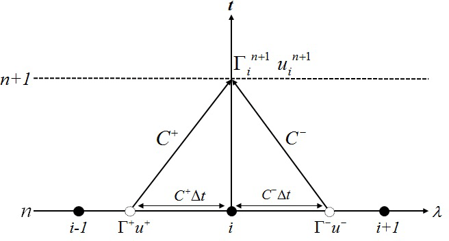
Figure 1 Space–time diagram showing the characteristic curves C^± where black points represent the grid points, white points represent the values Γ^± and u^± at time n to be interpolated to find Γⁿ⁺¹ and uⁿ⁺¹.

The equations for the coordinates are solved using the fractional step method. Following this method, the source term given by

$$\begin{array}{}\text{(13)}& {\displaystyle }{\displaystyle \frac{\partial U}{\partial t}}+S=\mathrm{0}\end{array}$$

is added to the solution obtained for Eqs. (4) and (10) . For the source term, central finite differences are used to solve the bathymetry term while the remaining values (cosine, tangent terms) can be solved analytically at each grid point since the variables are known straightforwardly.

In order to validate the implementation of the numerical methods for the SSWEs, we used the benchmark described in Kirby et al. (2013), where an initial Gaussian wave is propagated on an idealized sphere with water depth h=3000 m. Results after 5000 s show good agreement with the results reported which confirms the accurate propagation of the wave on the sphere and the effects of the curvature and Coriolis force.

3.2 Run-up calculation

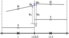
The Cartesian SWEs are solved in specific areas of just a few kilometers where inundation has to be calculated. For this case we use a finite volume implementation (Bradford, 2002; LeVeque and George, 2014) briefly described here. The surface gradient method (SGM) (Zhou et al., 2001) is utilized to solve the SWEs. This method uses the data at cell centers to determine the fluxes. In general, depth gradient methods cannot accurately determine the water depth value at cell interface, since effects of the bed slope or small variations in the free surface cannot be determined accurately. These inaccuracies are spread during the computation, resulting in an incorrect simulation of the inundation. In order to overcome this, the SGM uses a constant water level H. Figure 2 depicts the stencil for the water-depth reconstruction. By using the constant H as the total water depth at the cell interface (i+0.5) instead, the water depth be can determined accurately. In order to reconstruct the water depth, the following expression is used:

$$\begin{array}{}\text{(14)}& {\displaystyle }{h}_{L,Ri+\mathrm{0.5}}=\max \left(H_{L,Ri+\mathrm{0.5}}-{\stackrel{\mathrm{‾}}{z}}_{i+\mathrm{0.5}},\mathrm{0}\right),\end{array}$$

where $\stackrel{\mathrm{‾}}{z}$ is given by

$$\begin{array}{}\text{(15)}& {\displaystyle }{\displaystyle }{\stackrel{\mathrm{‾}}{z}}_{i+\mathrm{0.5}}=\left(z_i+z_{i+\mathrm{1}}\right)/\mathrm{2}.\end{array}$$

Figure 2 Reconstructed water depth h_L,R for inundation (LeVeque and George, 2014).

A MUSCL scheme (Yamamoto and Daiguji, 1993) is used to find the flux value, while local Lax–Friedrichs (LeVeque, 2002) is used to solve the bed slope source term. For the time integration, a third-order TVD Runge–Kutta scheme was used. This method is nonconservative; however, in tests the difference on mass conservation has shown to be almost negligible. Lastly, the bottom friction is computed using Manning's formula.

This run-up implementation assumes a thin film of water on land defined as ε. This parameter, set much smaller compared to the wave height, allows the computation of the wave inundation over land while keeping it stable. If the water height is less than ε (i.e., h<ε) then the height value is fixed as ε and the momentum is set as rest (i.e., hu$=\mathit{\text{hv}}=\mathrm{0}$) on that grid point. This implementation has proven to be robust and stable under different benchmarks and simulations (Vincent et al., 2001). This numerical-method implementation together with a slope limiter produces a monotone scheme that preserves water positivity.

The one-dimensional dam break benchmark (Stoker, 1992) was used to compare the results with its analytical solution and good agreement was found. The shock wave was successfully captured for different initial water heights.

The parabolic bowl problem proposed by Thacker (1981) was also used to compare the accuracy of the inundation. The bottom bathymetry is given by

$$\begin{array}{}\text{(16)}& {\displaystyle }{\displaystyle }z\left(r\right)=-D_{\mathrm{0}}\left(\mathrm{1}-{\displaystyle \frac{r^{\mathrm{2}}}{L^{\mathrm{2}}}}\right),\end{array}$$

while the water height at a time t can be found from the analytical solution

$$\begin{array}{ll}{\displaystyle }& {\displaystyle }H(r,t)=D_{\mathrm{0}}\left({\displaystyle \frac{{\left(\mathrm{1}-A^{\mathrm{2}}\right)}^{\frac{\mathrm{1}}{\mathrm{2}}}}{\mathrm{1}-A\cos \mathit{\omega }t}}-\mathrm{1}-{\displaystyle \frac{r^{\mathrm{2}}}{L^{\mathrm{2}}}}{\displaystyle \frac{\mathrm{1}-A^{\mathrm{2}}}{\left(\mathrm{1}-A\cos \mathit{\omega }t\right)}}\right)\\ {\displaystyle }& {\displaystyle }r={\left(x-L_x/\mathrm{2}\right)}^{\mathrm{2}}+{\left(y-L_y/\mathrm{2}\right)}^{\mathrm{2}}\\ {\displaystyle }& {\displaystyle }\mathit{\omega }=\sqrt{\mathrm{8}g{D}_{\mathrm{0}}/L^{\mathrm{2}}}\\ \text{(17)}& {\displaystyle }& {\displaystyle }A={\displaystyle \frac{{\left(D_{\mathrm{0}}+\mathit{\eta }\right)}^{\mathrm{2}}-D_{\mathrm{0}}^{\mathrm{2}}}{{\left(D_{\mathrm{0}}+\mathit{\eta }\right)}^{\mathrm{2}}+D_{\mathrm{0}}^{\mathrm{2}}}}.\end{array}$$

We use these parameters $L_x=L_y=\mathrm{8000}$, L=2500, D₀=1 and η=0.5. Two grid sizes were used for testing, 80×80 and 160×160 cells. Figure 3 shows the oscillating water in the bowl at different times. As it can be seen, the inundation method is able to capture the analytical solution of the water height well as it evolves in time on the different grid sizes. Measurements on this tests showed a third-order reduction of the error as the value ε was decreased.

3.3 Tsunami source model

TRITON-G focuses on propagation and inundation while relying on external parameters for the generation stage. In order to start a simulation, the initial condition is provided directly by RIMES using their preferred fault theory and model. In the generation process, a good initial source model is essential in order to obtain an accurate simulation. However, due to the complex nature of the source dynamics during an earthquake and the difficulty to track it in real time (as it happens), it is currently beyond our grasp to obtain these parameters precisely and instantly. For these reasons we opted for a coseismic deformation. This deformation is calculated from the theory of displacement fields proposed by Smylie and Mansinha (1971). Their objective was to provide a closed analytical expression that “facilitates the interpretation of near-fault measurements”. The expressions provided, valid at depth and surface, consist solely on algebraic and trigonometric functions that can be readily evaluated numerically based on a few source parameters like dip, strike, slip and length. These values are obtained from RIMES' databases online or loaded from a file. The original source generation code, provided by RIMES, was written for CPU and ported by us to GPU for this study.

3.4 Boundary conditions

Two kind of boundary conditions are used: open and closed. Open boundary set conditions to allow waves from within the model to leave the domain through an edge without affecting the interior solution. Closed boundaries, which keep the fluid inbound in the domain, physically prevent water flow across the edges. A wall boundary condition creates a total physical reflection when a wave hits a dry point.

In Eq. (1) the term cos θ in the denominators produces a singularity at the poles of the spherical coordinate system. When working on a complete sphere, special techniques and treatments are required to compute values over the poles without divergence. In this study, the domain chosen represents a portion of the Earth centered in the Indian Ocean and does not extend near the poles in any circumstance which permits us to avoid this pole singularity.

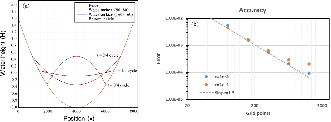
Figure 3 Parabolic bowl problem cross section with $\mathit{ϵ}={\mathrm{10}}^{-\mathrm{4}}$ on (a). Water depth error for parabolic bowl problem on (b).

The boundaries for the computational domain are set as open boundary condition at the south and east edges, and closed boundary condition at the north and west edges. All coastlines have wall boundary conditions except for the special cases where particular regions set as inundation are defined. In those cases a complete run-up is computed using the methods described in previous sections. Since the inundation method is relatively computationally intensive, using two kinds of boundaries for the coasts permits us to focus computational resources just in areas of interest.

The boundary between spherical and Cartesian coordinates that occur in specific areas where inundation is computed has no special treatment since the area covering the inundation consists, by design, of just a few kilometers (Fig. 5a). This makes the difference between meshes almost negligible and does not noticeably affect the result.

4 Tree-based mesh refinement and bathymetry

An efficient use of resources, memory and computation requires a mesh that covers areas of interest with high resolution only where desired but leaves the rest of the domain coarser. The concept of this approach is similar to that of the adaptive mesh refinement, initially introduced by Berger and Oliger (1984) and Berger and Colella (1989) in the 1980s as a method to solve partial differential equations (PDEs) on an automatically changing hierarchal grid, solving for a set accuracy on certain areas of the interest instead of unnecessarily overly refining the entire domain.

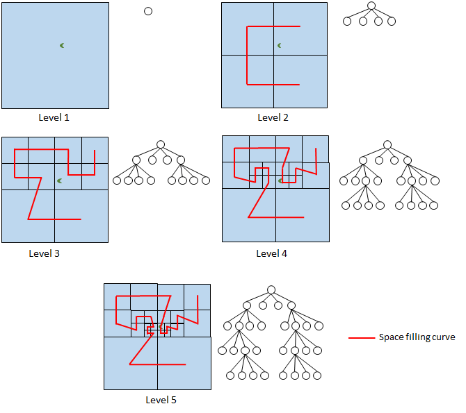
Figure 4 Tree-Based block refinement with quadtree structure and Hilbert space-filling curve for five levels.

To generate the mesh for the domain, we use a customized tree-based mesh refinement without the need of remeshing during simulation since the geometrical features remain unchanged. We briefly explain the process of tree-based refinement (Yerry and Shephard, 1991). Figure 4 illustrates this procedure using a moon-shaped green point as the area of interest. At each level, the domain and its tree structure, called quadtree, is presented. Initially just a quadrant and its quadtree root exist. Each quadrant represents a block of domain points. At level 2, one refinement has occurred and the original quadrant (father) is replaced by four new ones (children). By containing the same number of points as their parent quadrant, these children allow for greater resolution. Each child is represented as a leaf of the tree's root. Level 3 shows the refinement of two of the level 2 quadrants and are represented as two new leaves deeper on the quadtree. Focusing around the point of interest, levels 4 and 5 show the subsequent refinement of two quadrants of their respective previous levels. As it can be seen, each refined quadrant is replaced by four new ones, and these extend deeper into the tree. This process can continue recursively until reaching a desired goal, usually based on resolution or minimal error. Using this block refinement allows for greater resolution only around the points of interest while the quadtree data structure associated with it keeps track of the blocks' connectivity.

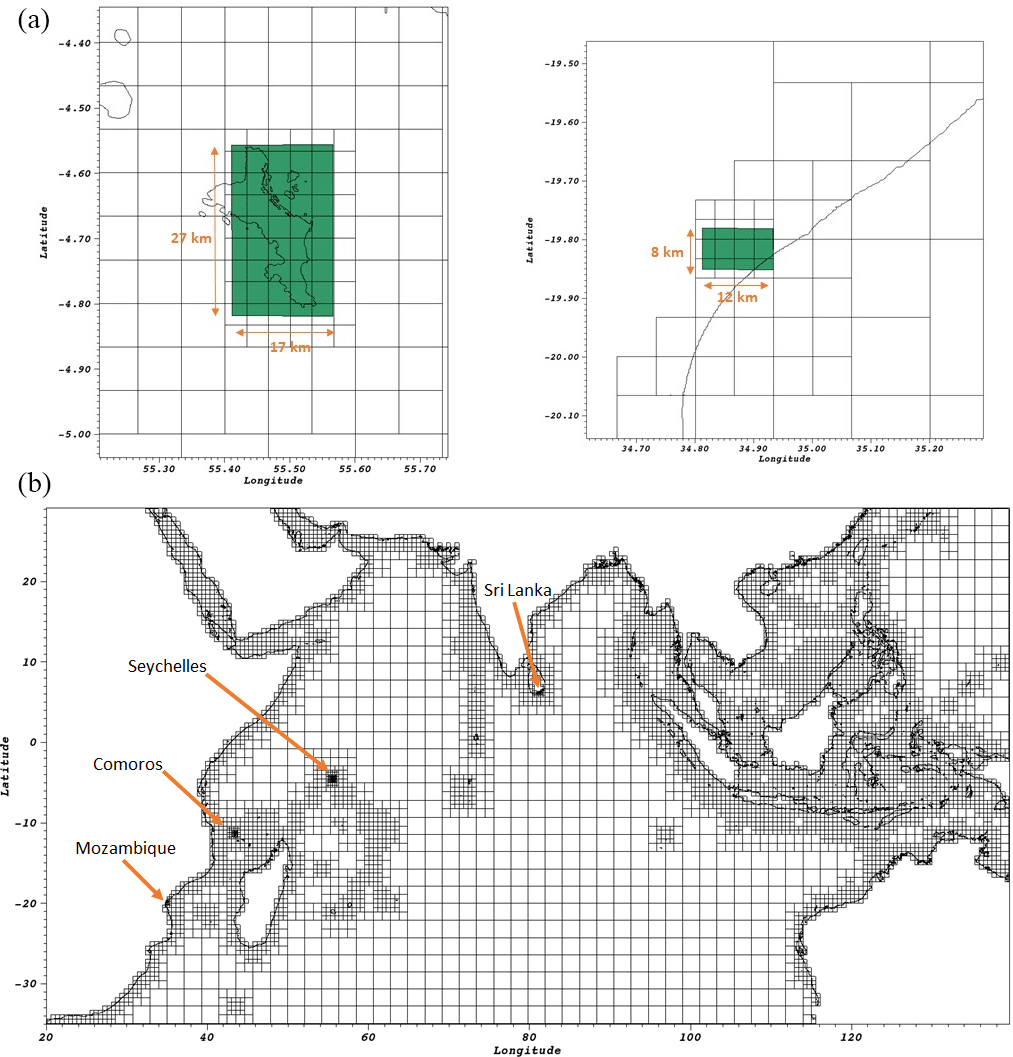
Figure 5 (b) Mesh refinement for Indian Ocean domain with four focal areas (FAs): Mozambique, Comoros, Seychelles and Sri Lanka. (a) Zoom on the Seychelles (right panel) and Sri Lanka (left panel) regions. FAs are highlighted in green.

The difference in spatial resolution between two adjacent levels is called the refinement ratio. For nested grids, this ratio is any positive integer. However using large integers tends to introduce inaccuracies in the computation. The existence of an abrupt change from one level to the next requires a special boundary treatment, especially when complex bathymetry or topography is involved. For tree-based refinement, this ratio is fixed as $\mathrm{\Delta }{x}_l/\mathrm{\Delta }{x}_{l+\mathrm{1}}=\mathrm{2}$, where l represents the block level and Δx the grid resolution. This constant and small ratio creates a smooth wave transition between levels.

4.1 Customized mesh generation

The domain used for this work represents a large portion of the Indian Ocean (Fig. 5), which initially consists of a uniform mesh of 56×30 blocks, each made up of 65×65 node-centered cells. Using the tree-based refinement, specialized customizations are developed to adapt it to our specific needs. In general, mesh-refinement methods utilize an error estimation as the rule to determine if a block should be refined; however, in this implementation the refinement depends on a target grid resolution combined with two factors: the block's distance from the coastline and the presence of a focal area.

Since the refinement rule's first factor depends on the distance of the block to the shoreline, the objective is to recursively refine blocks close to the coast until reaching a target high-resolution threshold, while blocks far in the ocean remain with a coarser resolution. This process involves two steps: determining the block's distance from the coast and checking if its distance is within refinement.

Accurately estimating the geo-distance between two points can be a complex task since the surface of the Earth is not a perfect sphere. However, for our refining purposes, a rough estimate is enough to determine the distances between the shoreline and the blocks. This is achieved by creating a signed distance function based on the level-set method. A detailed explanation of this procedure can be found in Fedkiw and Osher (2003). The distance function's zero level is represented by the cells along the shoreline (z=0). Positive distances represent cells on land while negative distances represent cells on the ocean. Using these distance values, each block is tested for refinement. Blocks with one cell or more within a certain distance from the coast, called refinement stripes, are flagged for refinement until they reach the fine-target resolution. The width of the refinement stripe is problem dependent and is input by the user based on their needs.

For this study the initial resolution at ground level 1 is 2 arcmin (an arcminute being 1∕60 of a degree, at Earth's equator equivalent to 1852 m) and the target finest resolution is 0.03125 arcmin (approximately 50 m), generating a total of seven levels. This block refinement process can accurately trace complex coastlines and focus high resolution only in the shores. A downside is the considerably large number of total blocks generated, over 230 000 in initial tests, which represents over 100 GB of memory storage.

In order to reduce the memory footprint, we used the fact that only certain regions need high resolution, which inspired us to use a second refinement factor named focal areas (FAs). This second factor is an additional constraint which consists of locating a convex polygonal area on the domain, which serves as a refinement delimiter. It is possible to locate more than one at a time, and since this is an additional constraint to the first refinement step, only blocks flagged for refinement at the first step need to be tested again. On this second test, a block is tested if it is inside or outside a focal area. If a block is completely outside the focal area, then it is unflagged for refinement. Only blocks partially or totally inside the focal area are refined. The process of determining if a block lies inside or outside a focal area is based on collision detection theory using the separating axis theorem (SAT). This is a well-known theorem applied to physical simulations (Szauer, 2017) and consists of a relatively light algorithm for 2-D, which allows us to test large number of blocks rapidly. A description of the SAT can be consulted in Moller et al. (1999) or Gottschalk et al. (1996). Since the focal area is an additional constraint, it can be toggled active after any chosen level. A specific number of levels can be refined without this constraint while the following are affected and delimited. Additionally, all dry blocks at Level 7 (highest resolution) that are inside a FA are considered inundation areas. This implies that run-up is computed on the coastlines instead of using a reflective boundary.

The last step in the mesh generation consists of the removal of land dry-blocks. Considering that tsunami inundations, with few exceptions, generally extend tens to hundreds of meters inland, it becomes clear that blocks located deep inland are unnecessary for the computation. For this reason all blocks whose cells' distances are larger than a land–distance threshold are considered land dry-blocks and deleted from the domain.

The complete result of the customized refinement in the Indian Ocean domain is shown in Fig. 5. The four focal areas used are located in Mozambique, Comoros, Seychelles and Sri Lanka. The focal area constraints start after level 3. This value is chosen to coincide with GEBCO's (The General Bathymetric Chart of the Oceans) 30 arcsec bathymetry, using the highest available accuracy for the coasts without needing to interpolate. The final result shows the refinement at higher levels limited to within the focal areas. All dry blocks exceeding the land–distance threshold of 10 km were removed from the mesh. This drastically reduced the number of blocks generated to 7849, while the memory needed to store them became less than 15 GB. This customized refinement procedure proved to be fast and efficient, taking just around a minute to produce the results. The meshes generated by TRITON-G can be either computed in real time or loaded from a repository at the beginning of the simulation.

4.2 Halo exchange

Blocks must exchange results with their neighbors after each time step for the next iteration. For this purpose they share a boundary layer in their adjoining sides. This layer, or halo, extends over the neighbor's grid and updates in one of three kinds of operations: copying, coarsening or interpolating.

If two neighbor blocks have the same level, then the halo is readily updated by exchanging values directly without any further computation; this represents a copying swap. If the neighbors are at different levels (l and l+1) then additional computation is required before the halo exchange. If the block's neighbor is one level up, then values for the halo are averaged down from the block with higher accuracy before swapping. This has a cascade effect of passing down better accuracy to blocks with lower resolution. The last case, interpolating, occurs when the block's neighbor is one level down. For this, the values for the halo are interpolated from the neighbor block using a third-order polynomial interpolation, similarly as in Eq. (9). The portion of the boundary stencil used for interpolation is shown in Fig. 6.

Figure 6 Halo interpolation stencil for the four edges: (a) west, south and (b) east, north.

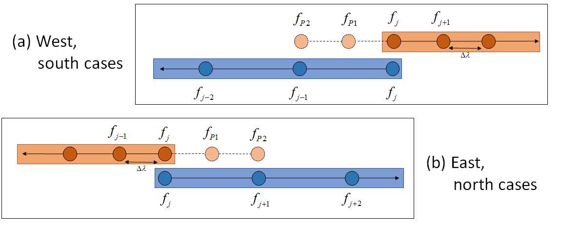
The new values for the halo for the north (N) and east (E) edges can be found from

$$\begin{array}{ll}{\displaystyle }& {\displaystyle }{f}_{P\mathrm{1}}^{\mathrm{N},\mathrm{E}}={\displaystyle \frac{\mathrm{1}}{\mathrm{4}}}\left(f_j+\mathrm{4}{f}_{j+\mathrm{1}}-f_{j+\mathrm{2}}\right)\\ \text{(18)}& {\displaystyle }& {\displaystyle }{f}_{P\mathrm{2}}^{\mathrm{N},\mathrm{E}}={\displaystyle \frac{\mathrm{1}}{\mathrm{4}}}\left(-f_j+\mathrm{6}{f}_{j+\mathrm{1}}-f_{j+\mathrm{2}}\right)\end{array}$$

since they are analogous orientations. For the south (S) and west (W) edges, similar expressions are used

$$\begin{array}{ll}{\displaystyle }& {\displaystyle }{f}_{P\mathrm{1}}^{\mathrm{S},\mathrm{W}}={\displaystyle \frac{\mathrm{1}}{\mathrm{4}}}\left(-f_{j-\mathrm{2}}+\mathrm{4}{f}_{j+\mathrm{1}}+f_j\right),\\ \text{(19)}& {\displaystyle }& {\displaystyle }{f}_{P\mathrm{2}}^{\mathrm{S},\mathrm{W}}={\displaystyle \frac{\mathrm{1}}{\mathrm{4}}}\left(-f_j+\mathrm{6}{f}_{j+\mathrm{1}}-f_{j+\mathrm{2}}\right).\end{array}$$

In order to avoid spurious waves that might be generated from interpolating the water height value h, constant water level H is used instead, and the original variable is recovered by using the relation $h=H-z$.

4.3 Topography and bathymetry

The data used in this study for bathymetry and topography comes from different sources. Initially, The General Bathymetric Chart of the Oceans (Oceans (GEBCO), 2017) database is used on the entire domain. GEBCO is freely available in 30 arcsec spatial resolution. When coarser resolution is needed, values are averaged from this database. On the contrary, if finer resolution is needed, a third-order interpolation is implemented to generate the new values. Where available, databases with more precise measurements are used to replace the original GEBCO database. For the focal areas in Mozambique, Comoros, Seychelles and Sri Lanka, RIMES' proprietary databases generated from field measurements were provided to us to estimate the inundation more accurately.

5 GPU computing

The introduction of C-language extension CUDA (NVIDIA, 2017a) by NVIDIA^® represented a disruption in the traditional way simulations were done. The availability to program general purpose GPU cards permitted researchers to no longer exclusively perform calculations on CPU. Due to the intrinsic parallelism of graphics, GPUs evolved to deliver hundreds and thousands of processors more in a card than CPUs. The main reason behind the exceptional performance of GPUs lies in the specialized design for compute-intensive, highly parallel computation, with transistors dedicated exclusively to processing as opposed to flow control and data caching. The latest NVIDIA Tesla cards P100, with Pascal architecture, have a peak performance of 9.3 Teraflops on single precision and 4.7 Teraflops on double precision (NVIDIA, 2017b). We take advantage of this technology to develop a full-GPU implementation to deliver fast forecasting results.

5.1 SSWE GPU kernels

CUDA provides kernels as a way to define functions that are executed in parallel on GPU. Each kernel launch is organized in a grid of blocks of CUDA threads. The clear analogy between CUDA blocks and mesh blocks provided a guide to organize the grid for GPU execution. The SSWEs are computed exclusively on GPU by processing the mesh blocks created during the domain refinement step and are stored in a structure of arrays on GPU global memory. Each mesh block has a size of $(\mathrm{65}+\mathrm{4})\times (\mathrm{65}+\mathrm{4})$, where the “4” corresponds to the total size of the halo. CUDA threads can be organized in any three-dimensional block configuration as needed for the problem. Since GPUs process threads in warps of 32, using multiples of this number is desirable to avoid performance penalties.

The kernel grid configuration for the SSWE is described briefly and shown in Fig. 7. CUDA threads are organized in two-dimensional blocks of size 64×4. The 64 threads in the x dimension cover the length of a mesh block requiring only one CUDA block. For the grid's y dimension, 16 CUDA blocks are set with four threads each, for a total of $\mathrm{16}\times \mathrm{4}=\mathrm{64}$ threads, covering the height of the mesh block. With this configuration, one CUDA block computes a portion equal in size of the mesh block and the 16 CUDA blocks cover the entire mesh block. Additionally, one CUDA thread computes one mesh block cell. The specific calculation of each thread varies depending on the block type (wet, dry); however, the configuration remains the same. In both cases, threads compute the governing equations described in Sect. 3.1. The main difference occurs in the case of a dry block; in this case, cells that represent land or coastline compute a reflective wall boundary.

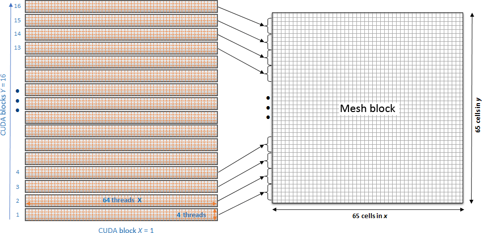
Figure 7 Mesh-block computation using CUDA kernels. Each CUDA block is made of 64×4 threads and computes a portion of the mesh block. One CUDA thread computes one mesh block cell.

To process all the mesh blocks, this two-dimensional CUDA block configuration is extended along the z direction as many times as mesh blocks exist. The computation of the 65th cells is done separately with a specialized kernel based on the SSWE kernel.

In the case of Cartesian SWE kernel, the grid chosen for this kernel is different than that of the kernel for SSWE. In this case, a mesh block is subdivided and covered by CUDA blocks of 16×16 threads. The excess of threads at the edges is not computed using a conditional limiting the grid size.

The source fault code was ported to GPU from the original C version. Due to the exclusively arithmetic operations and lack of a stencil memory access involved, a 20 times speed up was achieved, reducing the computation of the initial condition to just a few seconds.

Several kernel optimizations were applied in order to accelerate the model's time to solution. This includes using the latest CUDA version to take advantage of the latest compiler updates. To avoid branch divergence as much as possible parts of the numerical method were rewritten to eliminate conditionals. Precomputing terms that do not change in time like trigonometric terms depending on the longitude θ, storing them on arrays and reusing them during the simulation. Using built-in functions to compute complicated exponentials like those in the Manning formula. Although the optimizations provided speed up, no sacrifice was incurred on precision. All GPU computations are performed on double precision.

5.1.1 Halo update on GPU

Update of the halo region of each mesh block after each time step with the latest values from neighbor blocks represents three different kinds of exchanges: copying, coarsening or interpolating. These operations are performed entirely on GPU. Kernels designed for each kind of exchange were created. In order to efficiently process the block edges, three lists are generated containing the list of halos that require each operation. This way the kernels can be launched concurrently, and each focus on a different task minimizing the need for conditional divergences.

5.1.2 Specialized kernel types

By analyzing the domain's bathymetry, it is easy to notice that some mesh blocks contain only wet points while others are a combination of dry and wet points. This idea is used to replicate the SSWE kernel in two variations.

The first SSWE kernel, named Wet, is used to compute the free propagation of the wave on wet-only blocks. The second SSWE kernel, named Dry, is used to compute the wave propagation with coastline boundaries in wet–dry mixed blocks. The main difference in the code between them is the additional treatment for the wall boundaries at coastlines in the case of the Dry kernel. A third kind of kernel (Inundation), specializes in computing the run-up on dry blocks inside focal areas.

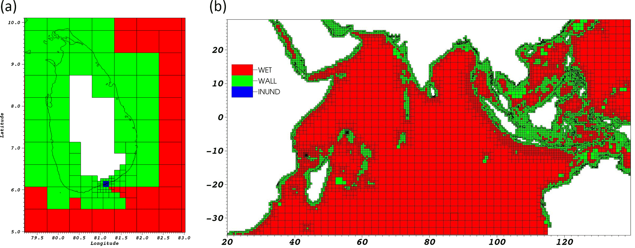
Figure 8 Mesh blocks colored by kernel type: Wet, Wall and Inundation. (a) Zoom over Sri Lanka FA to highlight the inundation kernels shaded in blue. (b) Kernel type distribution on the entire Indian Domain.

The result of the kernel assignment is illustrated in Fig. 8, where blocks flagged as wet are shaded in red, dry blocks are shaded in green and inundation blocks in blue. As expected dry blocks tend to extend where coastlines lie while wet blocks are spread out in the open ocean. When inside a focal area, dry-type blocks at level 7 are reflagged as inundation type. An example of this can be seen in the left image of Fig. 8 for the Sri Lanka FA, with inundation blocks in blue. Whereas a single kernel would be too complicated and inefficient to compute the entire domain, splitting down the computation in specialized kernels for each type of block not only provides a simpler way to process the blocks through lists, but also gives the ability to fine tune them independently for higher performance.

5.2 Space-filling curve and multi-GPU

In order to implement multi-GPU for further acceleration, first an appropriate domain partition must be chosen to guarantee an even workload among cards. Since a uniform mesh is not being used, this partition is nontrivial. Although block connectivity is kept using a quadtree structure, this does not provide information about the blocks ordering. For this purpose we use the space-filling curve (SFC) (Sagan, 1994) as a way to trace the blocks' ordering on the domain.

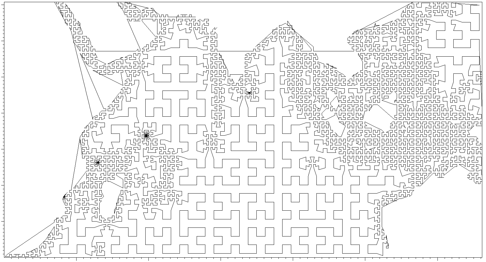
SFC is a curve that fills up multi-dimensional spaces and maps them into one dimension. It has many properties desirable for domain partition; it is self-similar and it visits all blocks exactly once. We use the Hilbert curve in this work since it tends to preserve locality, which keeps neighbors together and does not produce large jumps in the linearization like other curves tend to, such as the Morton curve. Figure 4 shows the Hilbert curve generation as a red line overlying the quadrants. It starts as a bracket on the first four quadrants, and with each spatial refinement, the bracket gets replicated subject to rotations and reflections to guarantee the characteristic of the curve. The result of generating a Hilbert SFC for the Indian Ocean domain is shown in Fig. 9. By using this curve as a reference, it is possible to establish the block ordering to partition the domain on even portions. The result of splitting the domain for eight GPUs is shown in Fig. 10, where each portion is represented by a different color. In this case, seven GPUs have a total of 981 blocks each, and the eighth GPU has a total of 982 blocks, making it a well-balanced partition. Different tests using one to four GPUs also achieved balanced partitions.

Figure 9 Hilbert space-filling curve for Indian Ocean domain with four FAs.

Introducing multi-GPU also introduces the need of a buffer communication between cards. In the current CUDA GPU memory model, global memory cannot be accessed between different cards. This exchange is achieved by preparing buffers on GPU memory, downloading to CPU memory, using MPI to exchange the messages and uploading the received buffer to GPU memory.

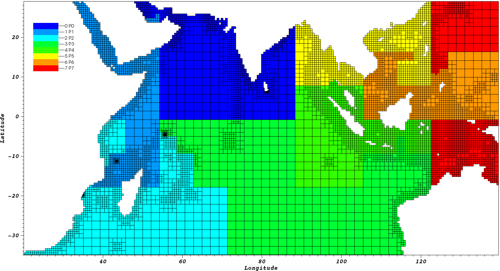
Figure 10 Indian Ocean domain partition for load balance for eight GPUs. Each color represents a different GPU.

In order to handle the communication structures and to produce buffers that do not represent a large communication overhead, we construct buffers following the user datagram protocol (UDP; Reed, 1980) design, a concept traditionally used in network and cellular data communication. In this way, it is possible to eliminate the need for communication look-up tables while at the same time making the buffer exchange smooth and simplified. As depicted in Fig. 11, the first step consists of collecting all the halos to be transferred in a single buffer on GPU memory. This buffer is designed like in UDP, with a header in front of every chunk of data. This header contains three bits of simple information: the destination block, the destination edge and the total size of its data. By including a simple 3-data header before the sent values, it is possible to organize the buffer in any way that packing and unpacking occurs smoothly and seamlessly.

By using this method, no extra memory is needed to store communication tables or exchange them between processors. A single-buffer transfer between processes drastically reduces the communication time as opposed to transferring each halo individually.

5.3 Variables and rendering output

The full workflow of TRITON-G is depicted in Fig. 12, where the GPU flow is composed of two parts: (1) the main simulation, which includes computing the fault source, wave propagation and inundation, and (2) the output compute and storage.

For post-processing analysis purposes, output for the wave maximum height, maximum inundation, arrival time, flux and gauges is created. These are computed during simulation and stored on GPU memory, then flushed to CPU when required by the user. A full-domain rendering at a regular frequency is also produced during simulation, while for the FAs, wave values at a much higher frequency are stored. These values are used for rendering at post-processing to avoid unnecessary output overhead.

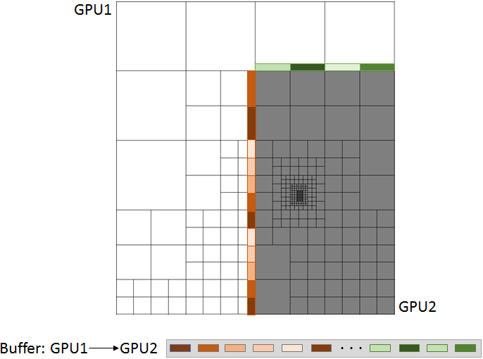
Figure 11 Multi-GPU communication. GPU buffer data collected and packed for a single communication.

Figure 12 TRITON-G computational flow; mem: memory.

Figure 13 Output overlap and optimization using Pipe.

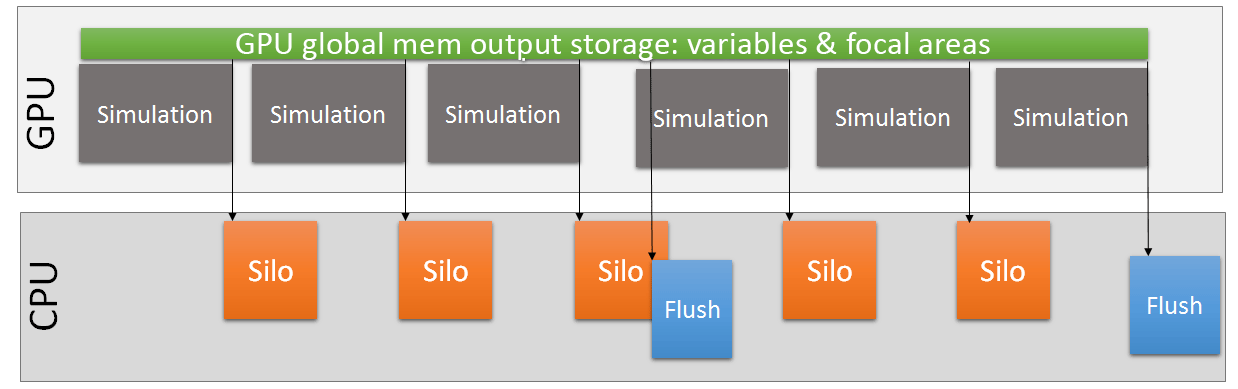
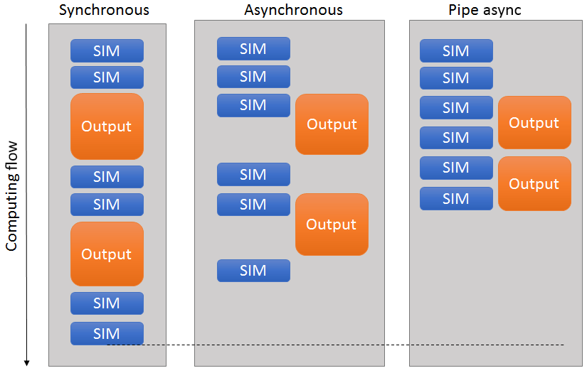
TRITON-G generates SILO format files (Lawrence Livermore National Laboratory, 2017) filled with values from all blocks to generate the rendering images. Even though the image generation for the entire domain is not very frequent, the process of generating a SILO file for such a large mesh represented a considerable overhead of around 15 % to 20 % of the total runtime. In order to minimize this unwanted effect, we took advantage of the piping mechanism. Pipe is a system call that creates a communication between two processes that run independently. In this way, a parent program can launch a child program, and both run completely different tasks at the same time without interrupting each other. Using this concept, first a utility to create the SILO files for the entire domain was created as a stand-alone application. During execution, TRITON-G calls this subprogram when a SILO file has to be written, running both simultaneously. Data between them are shared through the CPU shared memory. Figure 13 shows the advantage of implementing Pipe asynchronous output. Unlike traditional asynchronous output that relays on a large computational time to hide output, this Pipe method provides the ability to hide the output processing behind several computational time steps. The result is an almost total elimination of the output overhead. Measurements showed that the output process after optimization represented just 1 % to 2 % of the total time, practically removing the overhead.

The size of the output produced during simulation depends on user input parameters. For a 10 h simulation with an output frequency of 4 min for the entire domain, and 5 s for four FAs, the required memory storage is around 65 GB.

5.3.1 Subcycling implementation

A subcycling technique was introduced in order to increase the computational time step and further speed the computation up. Subcycling consists of setting a larger than the minimum time step as a global time step Δt, and making blocks with a smaller local time step cycle in substeps (ns) to match the global Δt. The time step Δt is calculated in each level using the Courant–Friedrichs–Lewy condition (CFL) (Courant et al., 1967). Initially the CFL number is set to 0.8 for this work.

A graphical illustration of the subcycling implementation is shown in Fig. 14. Blocks with the same number of subcycles (levels L1–L4) are grouped in a single list. A block at level 5 (L5) has a time step of Δt∕2, which implies that it requires two cycles to match the global Δt.

Figure 14 Illustration of the subcycling process for each level.

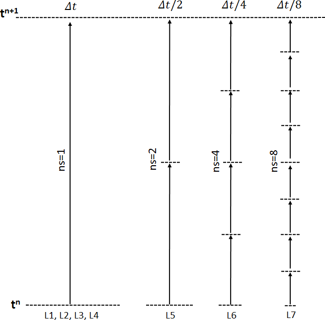
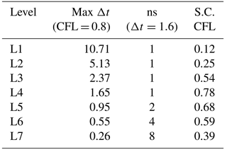
While in theory the larger time step increases speed, a potential downside is that too many blocks subcycling can create a large workload overhead, resulting in a slowdown of the whole computation. To avoid this, a global Δt of 1.6 s is chosen to subcycle only blocks with levels over level 4. The reason being, is that around 80 % of the total number of mesh blocks are level 3 and subcycling them would represent too large an overhead and would defeat the purpose of applying this technique. Table 1 gathers the CFL numbers per level after implementing the subcycling. The second column shows the maximum Δt allowed in each level using the initial CFL = 0.8. The third column shows the resulting number of subcycles per level (ns) and the fourth column shows the new CFL values obtained for each level. In all cases the new CFL values remain below 1 to guarantee stability.

Figure 15 GPU execution time with and without load balance.

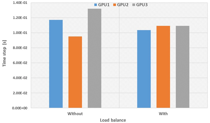
Table 1 CFL values used after introducing subcycling (S.C. CFL) for each of the seven levels. The second column shows the maximum Δt per level using CFL = 0.8 and the third column shows the number of subcycles (ns) required in each level when using Δt=1.6.

In general after a large Δt step, corresponding boundary conditions are interpolated in time to update the substeps. However, this procedure introduces an additional computational overhead. To pursue the fastest modeling possible, TRITON-G rescinds the boundary generation and instead uses the available boundary values at time n. Based on the benchmark and hindcast comparison, this decision proved to be acceptable based on the good agreement and accuracy of the results.

Introducing this subcycling technique varies the GPU load initially created since a single block might be computed more than once. In order to guarantee load balance, two weights are applied to the space-filling curve. The first weight takes into account the different type of block, and the second the number of subcycles. Each block gets attributed a weight during the SFC generation equal to the number of subcycles it requires. This approach for the domain partition allows us to create a fair work rebalance on the GPUs. The effect of implementing the weighted load balance can be seen in Fig. 15, where GPU execution times per time step are presented, with and without load balance. Implementation of the subcycling technique showed a speedup of around 15 % in the total wall-clock runtime.

5.3.2 Runtime performance

Several tests to estimate the performance of TRITON-G were done. Results ran on the supercomputer Tsubame 3.0 (Tsubame, 2017) are presented, with Intel Xeon E5-2680 2.4 GHz ×2, RAM 256 GB, NVIDIA Tesla P100 (16 GB) ×4/node, CUDA 8.0, gcc 4.8.5, Openmpi 2.1.1 and Omni-Path HFI 100 Gpbs network.

As comparison, results on a second machine are also presented using four Tesla K80 (12 GB ×2) cards in a node (eight GPUs in total). GPUs are connected through PCI-Express 3.0, Intel Xeon CPU E5-2640 @ 2.6 GHz, RAM 128 GB, CUDA 8.0, gcc 4.7.7 and Openmpi 1.8.6. These performance tests serve to show very good portability of our program on different hardware, older and much newer, without requiring changes or producing problems.

Figure 16 Computing breakdown shown in percentage.

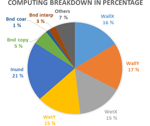
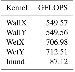
The breakdown of the main parts of the simulation using three GPUs is shown in Fig. 16, where Inund stands for inundation kernel, Wall stands for the Wall kernel, Wet for the Wet kernel and X and Y for the direction of the computation equivalent to longitude and latitude respectively. The process of updating the halos, presented in the graph as Bnd, represents only 9 % of the total running time. It can be seen that the Wet and Wall kernels have similar performance despite the fact that the wall includes additional treatment for the coast boundaries. Since this treatment consists of many conditionals and they were replaced during optimization, it is understandable that the performance is similar. The slice Others includes several values; most importantly communications which represents around 1.5 %–2.0 % of the total running time. Performance of the main kernels on one GPU in floating point operations per second (FLOPS) is gathered in Table 2.

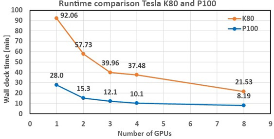
Results for runtimes using Tesla P100 cards and Tesla K80 cards are presented in Fig. 17 for one to four and eight GPUs. For this test, 10 h were simulated on the mesh initially generated for the Indian Ocean domain (Fig. 5). All runtimes measurements include output time.

Table 2 Kernel performance for one GPU in GFLOPS

A comparison between both GPU cards shows a speed up of almost four times from the older K80 cards to the latest P100 on Tsubame 3.0. In our collaboration project with RIMES an objective to complete this test under 15 min was set, which could be fulfilled by using three to eight GPUs in this configuration. Runtime for three GPU with K80 cards was 39.96 and 12.1 min with P100 cards.

A saturation is noticeable in Fig. 17 as the number of GPUs are increased. A possible reason for this phenomenon is related to the increase of buffer preparation, packing–unpacking and the communication exchange. Using the same domain size for all cases is another possible reason. Having fewer blocks on each GPU generates lower occupancy which might degrade performance. However, having met this study's time-to-solution objective of less than 15 min, no further optimization was deemed necessary.

By measuring the time required for the first wave to arrive in the focal areas, it was found that for Sri Lanka, using four GPUs for just 2 min wall-clock time is required to generate the results of the inundation. The real tsunami wave took approximately 2 h to propagate from the initial source to Sri Lanka, obtaining simulation results faster than real time. This gives authorities sufficient time to make decisions regarding evacuations.

Figure 17 Wall-clock comparison of 10 h simulation on Tesla K80 and Tesla P100.

6 Tsunami inundation benchmark comparison

In order to compare the numerical results of TRITON-G with existing benchmarks and test its ability to estimate inundation, we present the results obtained using the main benchmark tests proposed in the National Tsunami Hazard Mitigation Program workshop (NTHMP, 2012). Results from other models participating in the workshop can be consulted in that reference. In this section, the comparison of the benchmark “1993 Hokkaido–Nansei–Oki (Okushiri) field” is shown. Further comparison results with benchmark problems 4, 6 and 7 (abbreviated as BP4, BP6, BP7) can be found in the “Appendix”.

A detailed description of the benchmarks can be found in NTHMP (2012) and the data needed for them can be found in the repository https://github.com/rjleveque/nthmp-benchmark-problems (last access: 13 September 2018). For completeness we give a brief explanation of the benchmark and the tasks it involves.

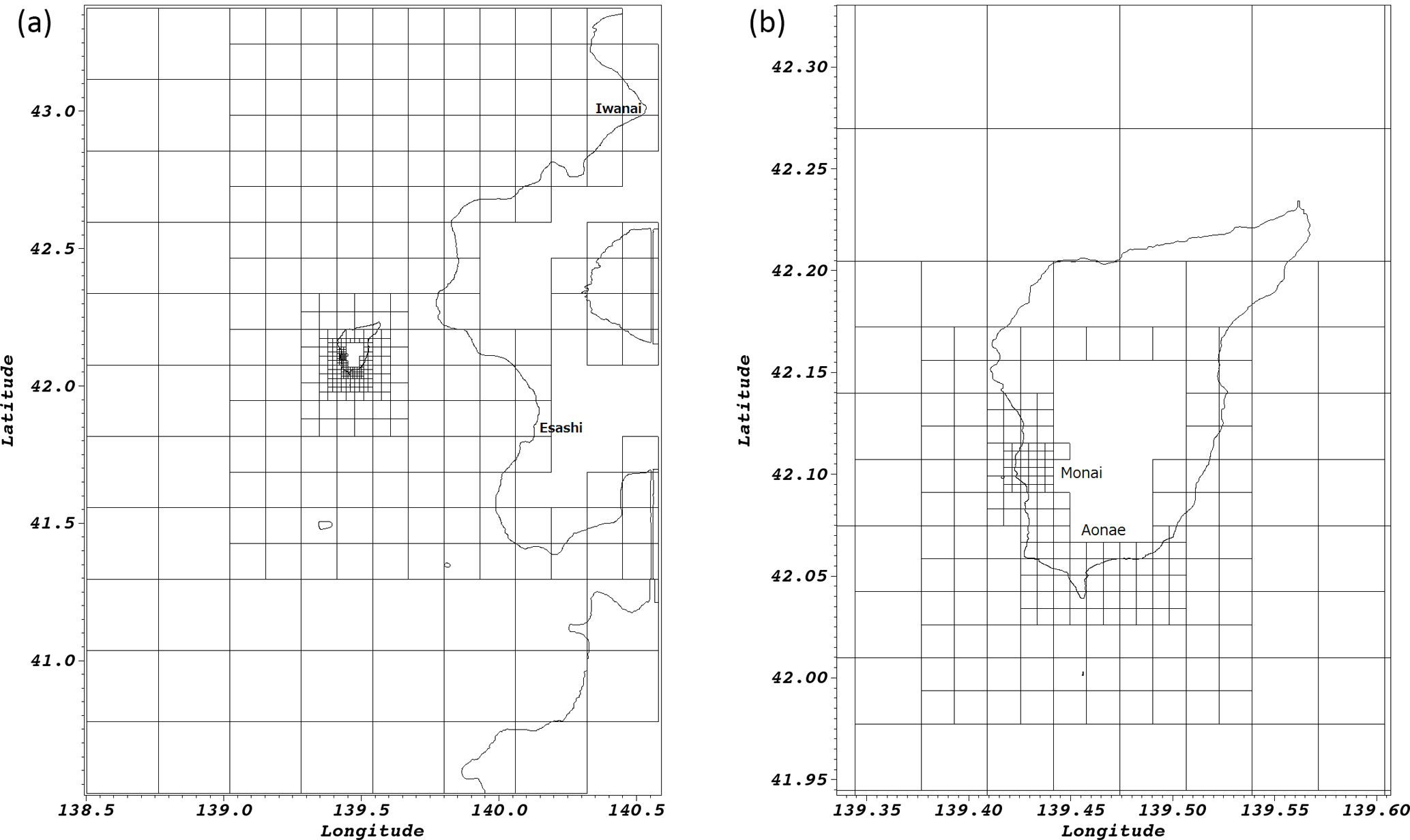
Figure 18 (a) Entire domain-refined mesh containing seven levels. (b) Zoom on Okushiri island. Higher resolution used around Monai Valley at level 7 (7 m approx.) and Aonae region at level 6 (14 m approx.).

6.1 Benchmark problem no. 9: Okushiri Island tsunami – field

This benchmark problem (BP9) is based on the data collected from the M_w=7.8 Hokkaido–Nansei–Oki tsunami around Okushiri Island in Japan in 1993. The goal is to compare computed model results with the field measurements.

6.1.1 Problem setup

The following parameters were used for the computation.

• Bathymetry is taken from databases provided by NTHMP (2012), interpolated where necessary.

• The CFL is 0.9.

• The simulated time is 60 min.

• The initial condition is source generated from the database provided by the DCRC (Disaster Control Research Center) Japan solution DCRC17a, described in Takahashi (1996).

• The boundary conditions are open boundaries at the four domain edges.

• For friction, the Manning coefficient is set to 0.02.

• For the computational domain, a mesh refinement is used (shown in Fig. 18). Seven levels are used in total. The resolution of base level 1 is 450 m and the resolution of level 7 is approximately 7 m. Dry blocks that did not take part in the computation were removed in the mesh generation process.

6.1.2 Tasks to be performed

This benchmark requires the following tasks to be performed:

1. compute run-up around Aonae;

2. compute arrival of the first wave to Aonae;

3. show two waves at Aonae approximately 10 min apart (the first wave came from the west, the second wave came from the east);

4. compute water level at Iwanai and Esashi tide gauges;

5. maximum modeled run-up distribution around Okushiri island;

6. modeled run-up height at Hamatsumae; and

7. modeled run-up height at a valley north of Monai.

Figure 19 Inundation map of Aonae region with 4 m contours of bathymetry and topography.

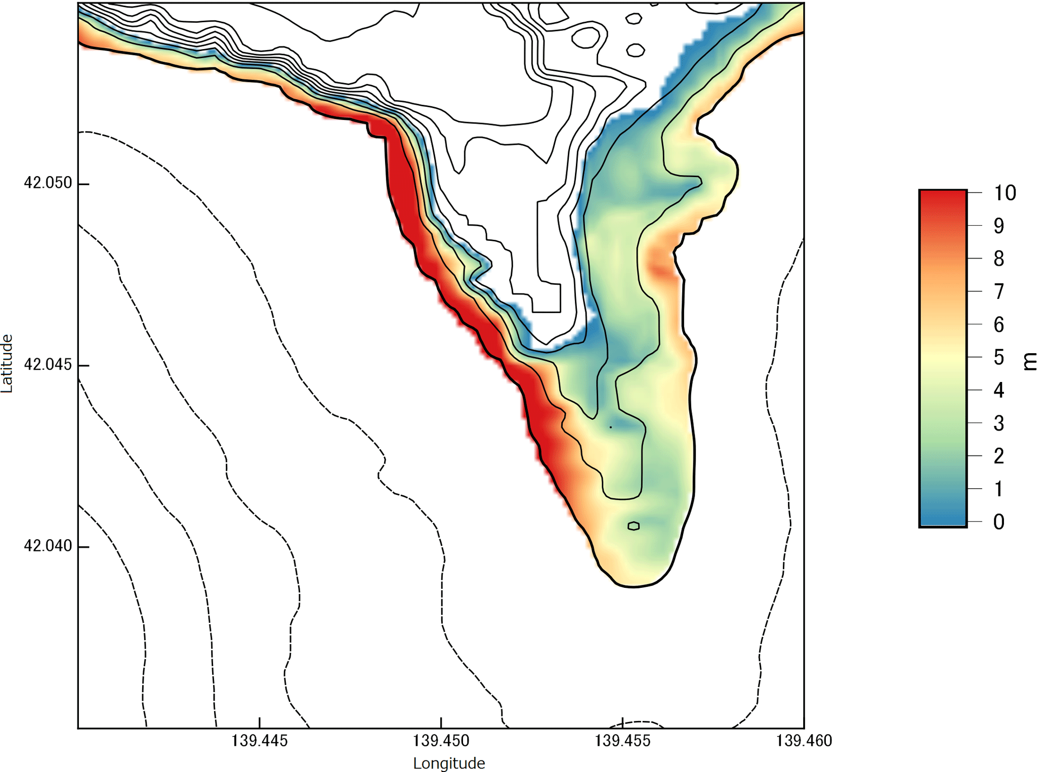
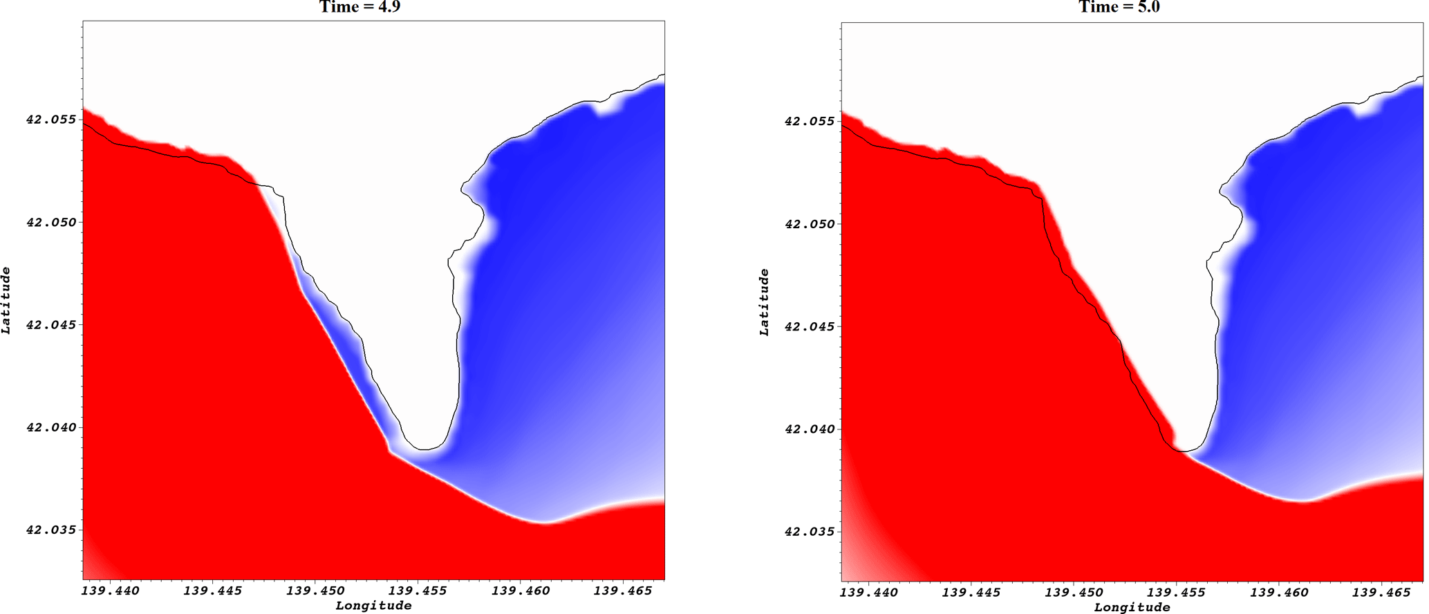
Figure 20 Arrival wave at Aonae peninsula coming from the west, snapshots of the wave at times 4.9 and 5.0 min after tsunami generation.

6.1.3 Numerical results

In this section we present the numerical results obtained with TRITON-G for benchmark problem no. 9.

Run-up around Aonae

The maximum inundation around Aonae peninsula modeled during the simulation is shown in Fig. 19. Contours every 4 m are drawn to show the outline of the topography. Maximum inundation height computed was nearly 15 m but the scale used is set to the upper limit of 10 m to highlight the areas where major inundation occurred.

The west side of the peninsula received the impact of the first wave, which produced the largest inundation height. Maximum values of nearly 15 m were obtained in the simulation. Despite a relatively lower inundation height in the east side of the peninsula, deep penetration was found due to the flatter topography in this area. The inundation on the east side was mainly produced by the second wave coming from the east. The south side of the peninsula experienced the impact of both first and second waves and run-up of over 12 m was estimated.

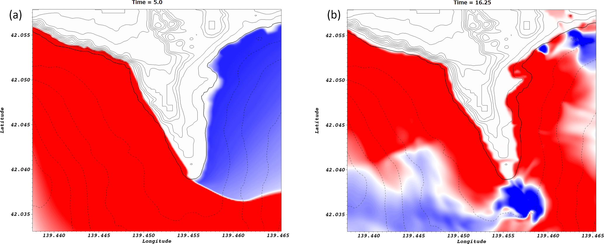
Figure 21 Two waves arriving at Aonae peninsula. (a) First wave coming from the west arrived at around t=5 min. (b) Second wave coming from the east arrived at around t=16 min.

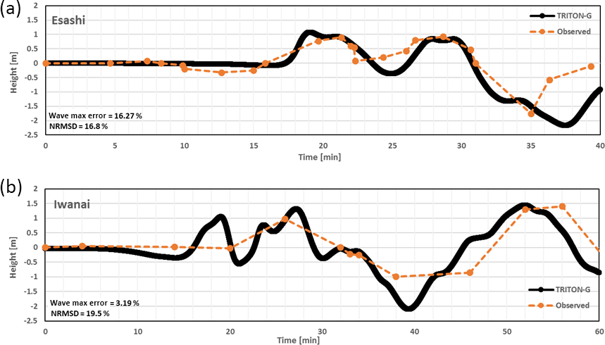
Figure 22 Water level comparison between observations and TRITON-G results for Esashi (a) and Iwanai (b) tide gauges.

Arrival of first wave to Aonae

The arrival of the first wave at Aonae peninsula is shown in Fig. 20. This wave is coming from the west. Snapshots are approximately 5 s apart at times 4.9 and 5.0 min to illustrate the wave arrival. From these snapshots, we estimate that the wave made impact at around 5 min after the tsunami generation.

Two waves arriving at Aonae

The two waves arriving at Aonae peninsula are shown in Fig. 21. The first one came from the west (Fig. 21a) and made impact at around 5.0 min after the tsunami generation. The second major wave to hit the peninsula came from the east and made impact at around 16 min (Fig. 21b). Slightly over 10 min separated the first and second wave.

Tide gauge comparison at Iwanai and Esashi

Comparison between computed and observed water levels at Iwanai and Esashi tide gauges is presented in Fig. 22. The arrival time of the computed wave shows good agreement for Esashi station. The computed wave positive and negative phases also follows the observed values rather well. In the case of Iwanai station, the arrival time is slightly sooner than the observed; however, the observed wave phase is followed generally well in the computed results. The discrepancies between observed and computed values can be attributed to several reasons. Inaccuracies in the source used for the initial condition can greatly influence the result. Additionally, the lack of realistic bathymetry including man-made structures around the area can affect the results as well.

Inserted in each panel of Fig. 22 are the estimated errors for the gauge comparison. The maximum wave amplitude error for Esashi station is 16.27 % and for Iwanai 3.19 %. These are considerably lower than the mean values obtained by the models reported in the workshop (NTHMP, 2012) of 43 % and 36 %, respectively. Although no values are reported in NTHMP (2012), the normalized root-mean-square deviation (NRMSD) error is also estimated for our model and included in the panels. Both values are under 20 %.

Maximum run-up around Okushiri

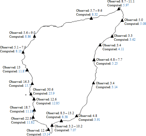
The computed maximum run-up distribution around Okushiri Island is shown in Fig. 23. Observations were taken from Kato and Tsuji (1994). Good agreement is found between observed and computed values around the coast. Most values are within the observed range or within a small difference from the field measurement. The simulation seems to capture well the variations that occurred along the coast.

The model could simulate well the maximum run-up observed around Monai valley within a reasonable 15 % error. The major differences are found in the southwest side of the island, where run-up values were underestimated with larger difference. The discrepancies could be explained by the use of different grid around the island coast. Additionally, the lack of an accurate high-resolution bathymetry database everywhere can also influence the computed values as well as an inaccurate initial condition.

Run-up height at Hamatsumae

The maximum inundation map for Hamatsumae region is shown in Fig. 24. Topography and bathymetry contours are outlined every 4 m. A grid resolution of approximately 14 m was used for this region. Near the center of the region and to the east, run-ups of nearly 16 m were computed. Additionally, inundation values ranging from 8 to 10 m were obtained which match well with field observations.

Run-up height at a valley north of Monai

The maximum inundation map for the valley north of Monai is shown in Fig. 24. Topography and bathymetry contours are outlined every 4 m. A grid resolution of approximately 7 m was used for this region. Inundation of around 26 m was computed, relatively close to the 30.6 m observed in the field.

Figure 23 Computed and observed run-up values in meters along the coast of Okushiri island.

7 Case study

In order to compare and validate the results of TRITON-G under a real tsunami scenario we use the hindcast of the 2004 Indonesian tsunami. Results for propagation, gauges and inundation comparison are presented.

7.1 Indonesian 2004 tsunami hindcast

This event occurred at 07:58 LT on 26 December 2004, with a magnitude of M_w=9.0 generated by the subduction of the Indian plate by the Burma plate. Nearly 1600 km of fault was affected around 160 km off the coast of Sumatra (Titov et al., 2005). This massive earthquake generated a large tsunami that spread over the Indian Ocean in the following hours.

The tsunami wave propagation computed by TRITON-G is depicted in Fig. 26. Each subsequent snapshot represents 3 h after the earthquake's main event. A synoptic qualitative comparison with existing field surveys and simulations confirmed a correct propagation of the initial wave train; however, to check the validity of the results, two kind of comparison are presented for tide gauge records and for inundation map simulations.

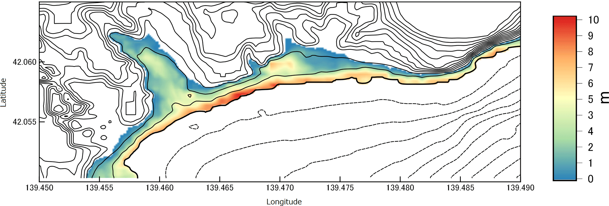
Figure 24 Inundation map of Hamatsumae region with 4 m contours of bathymetry and topography.

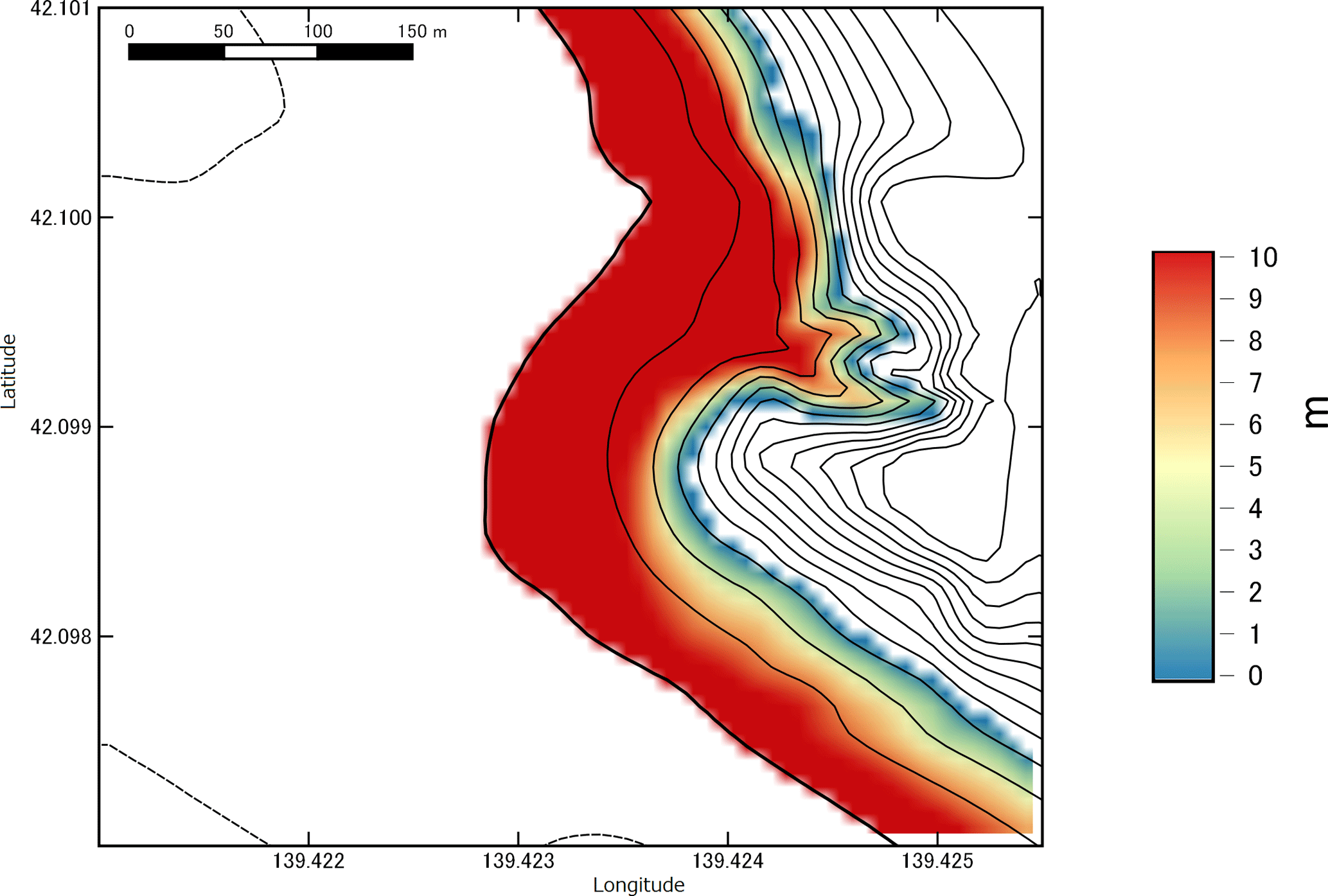
Figure 25 Inundation map for the valley north of Monai with 4 m contours of bathymetry and topography.

7.1.1 Tide gauge comparison

To check the correctness of the wave propagation, buoys located in different parts of the Indian Ocean were used to compare TRITON-G results. These buoys measure the ocean sea level at regular intervals and serve as a critical factor to determine tsunami wave arrival times and heights. Gauges recorded at the moment of this event were obtained from NOAA's tsunami events database and inundation maps were obtained through RIMES. Results from RIMES' previous operational model are also included for comparison. Their previous model was based on a customization of TUNAMI (Srivihoka et al., 2014) to include four nested grids with fixed resolutions of 2 arcmin, 15 arcsec, 5 arcsec and approximately 1.67 arcsec.

Results for five stations are shown: Diego Garcia (Fig. 27a) in an atoll in the Chagos Archipelago, located at 7^∘30^′ N 72^∘38^′ E; Male (Fig. 27b) near the Maldives islands, located at 4^∘18^′ N 73^∘52^′ E; Gan (Fig. 27c) near the Maldives islands, located at 0^∘68^′ N 73^∘17^′ E; Colombo (Fig. 27d) in Sri Lanka, located at 64^∘93^′ N 79^∘83^′ E; and Point La Rue (Fig. 27e) near Seychelles, located at 4^∘68^′ S 55^∘53^′ E.

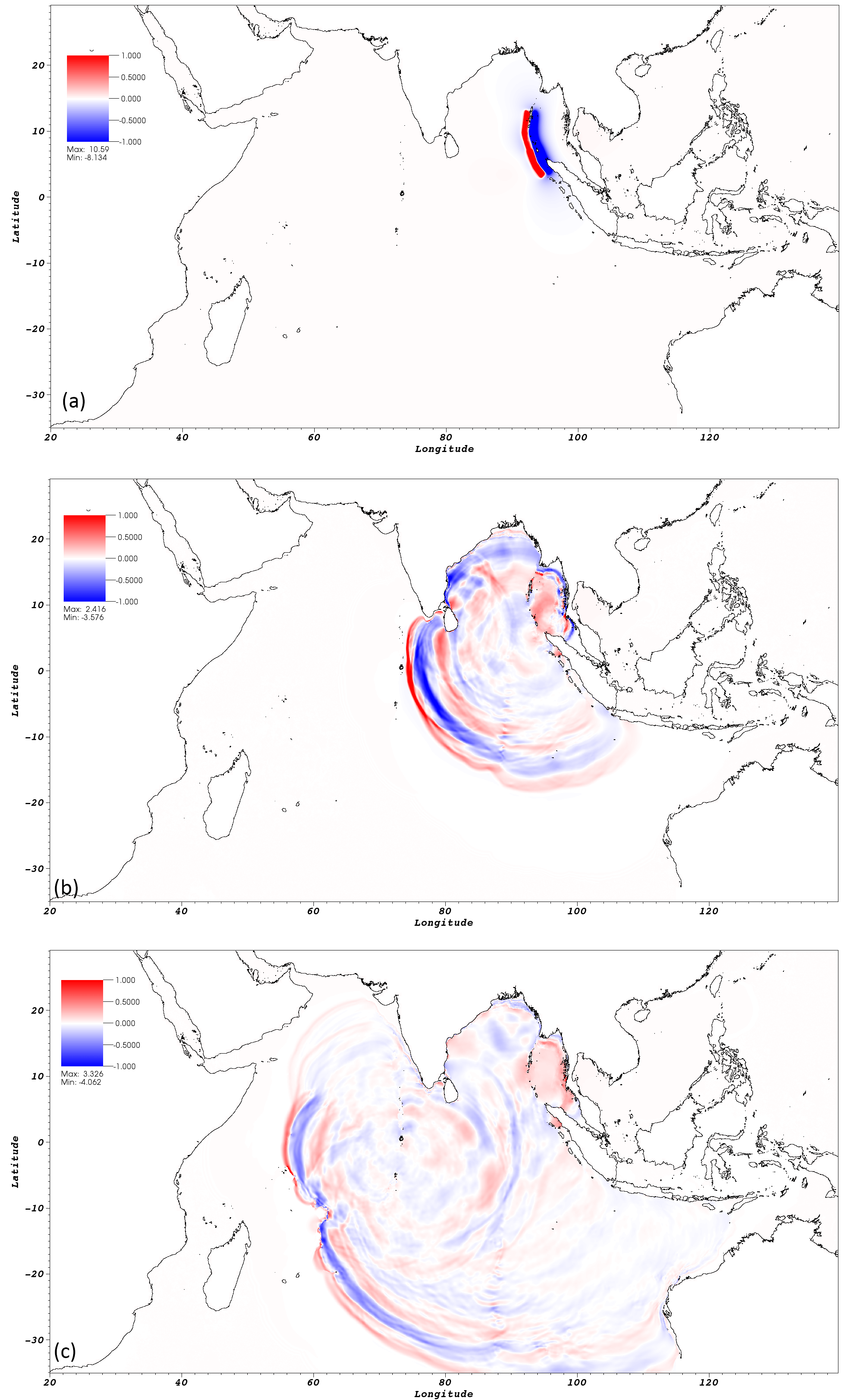
Figure 26 Snapshots every 3 h (a)–(c) of the Indonesian 2004 tsunami propagation simulated by TRITON-G. (a) Time = 0 h. Initial source in Sumatra. (b) Time = 3 h. (c) Time = 6 h.

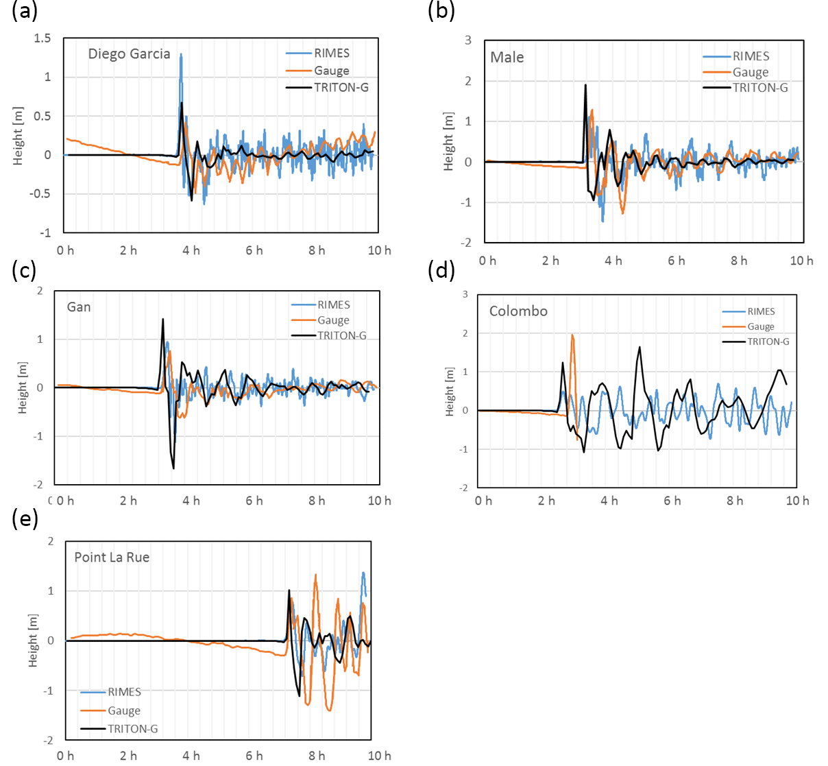
Figure 27 (a) Comparison of arrival wave at Diego Garcia, tide gauge and model results. (b) Comparison of arrival wave at Male, tide gauge and model results. (c) Comparison of arrival wave at Gan, tide gauge and model results. (d) Comparison of arrival wave at Colombo, tide gauge and model results. (e) Comparison of arrival wave at Point La Rue, tide gauge and model results.

The comparison between the tide gauges TRITON-G and RIMES' model based on TUNAMI are shown in Fig. 27. As it can be seen, the arrival times are in good agreement with the measured ones. The main event peaks are also reproduced in all cases with the crests' signs in accordance with the measured values. The effect of the tide is not considered in the current model, which explains the height differences at initial times in the results. In the case of Male, three of the first peaks were also estimated in the simulation. The case of Diego Garcia also serves as a test for long propagation, since it is located around 2700 km away and there is no topography between source and station. This makes it a good way to validate that the wave is properly propagated at the right speed, and no effects of diffusion on the wave height are present. Diego Garcia and Colombo (which recorded only around 3 h before being damaged) are two examples of more accurate and closely obtained results than the previous model used at RIMES, where a closer height to the measured peak was obtained. Point La Rue also represents a good test for long propagation of the TRITON-G numerical model since the location is over 4500 km from the source, and the wave has traveled over complex bathymetry and reflected on multiple coastlines. However, the arrival time is still in good agreement as is the wave arrival peak height. No effect of wave main peak diffusion is noticeable.

The arrival time differences of a few minutes between measurement and TRITON-G simulation can be partly explained by the location of simulated gauges. Even though the main events could be reproduced, a tendency to overshoot is noticed; nonetheless, this did not affect the ability of the model to transport the wave along far distances, and in no case was an arrival wave sign reported incorrectly. We briefly discuss three main reasons for the difference in arrival height and wave oscillation after the main event. The first is related to bathymetry and topography. Although databases for bathymetry and topography with good accuracy are available, these are still far from representing in detail the real shape of the ocean's bottom and topography. This difference makes it challenging to reproduce the wave reflections on coasts and the effects of traveling through the ocean bottom in a completely realistic way. Based on this, it is expected that some differences are found in the wave reflections and oscillations. A study about the influence on bathymetry resolution can be found in Plant et al. (2009). The second reason relates to the dependence of every tsunami model on a good and accurate initial condition to obtain good simulations. The use of inaccurate initial fault sources can affect the resulting simulation especially in locations near the source. This is particularly challenging since it is not possible to precisely measure the ocean surface at the moment of a tsunami event. The third reason is related to dispersion. Waves traveling through the ocean bottom experience physical dispersion due to the effect of the bathymetry. In general, this dispersion is compensated by numerical dispersion introduced by the truncation error. However, TRITON-G utilizes a cubic interpolation upwind scheme that has the advantage of minimizing dispersion and diffusion. An almost homogeneous traveling train wave with a minimal dispersion effect is produced instead, reducing the possibility of seeing the higher oscillatory behavior of the arrival tsunami wave seen in the gauges. These kinds of discrepancies had been observed and reported on in several other operational models as well (Dao and Tkalich, 2007; Grilli et al., 2007; Arcas and Titov, 2006).

7.1.2 Inundation map comparison

A further validation for the TRITON-G model is to compute inundation in certain areas and compare it with field surveys or existing maps. Since inundation maps that are exactly measured do not exist, we present comparisons with RIMES' existing simulated inundation maps (RIMES, 2014) and post-tsunami field surveys. Two cases are presented: the first in Hambantota (Sri Lanka) and the second in Phuket (Thailand).

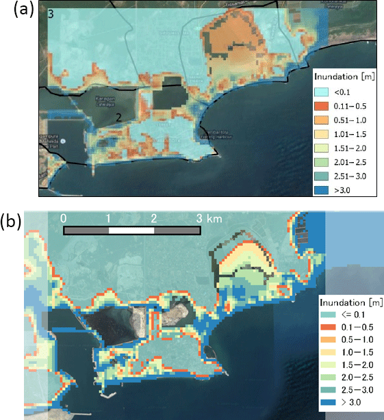
Figure 28 Inundation comparison for Hambantota, Sri Lanka. (a) RIMES model. (b) TRITON-G model.

The first inundation validation presented is the result for Hambantota in Sri Lanka. The inundation map for Hambantota generated by TRITON-G is shown in Fig. 28b. For comparison, we include in Fig. 28a panel the previous result obtained by RIMES in their report “Tsunami Hazard and Risk Assessment and Evacuation Planning – Hambantota, Sri Lanka” (RIMES, 2014).

Eyewitness accounts report the arrival time of the first tsunami wave around 09:00 LT the morning of the 26th, some 2 h after the initial earthquake in Sumatra. This coincides with TRITON-G's predicted arrival time of 2 h for this region. According to measurements done post-tsunami, it was determined that the arrival waves had heights of over 8 m and produced run-ups inland in certain areas of up to 2 km.

TRITON-G inundation results also show areas up the coastal bay where run-up produced inundation hundreds of meters deep in land, coinciding with the recounts. By comparing it with the result provided by RIMES, we found that both simulations show agreement with each other on the areas that experienced and did not experience inundation. The decisive factor that made some areas more prone to inundation than others was the topography. The arrival tsunami wave hit the coast with heights of around 8–10 m. Coastal areas that faced the ocean with higher topographic heights were spared from being inundated. On the contrary, coast shores that were practically flat were overtaken by the incoming wave as shown in the results.

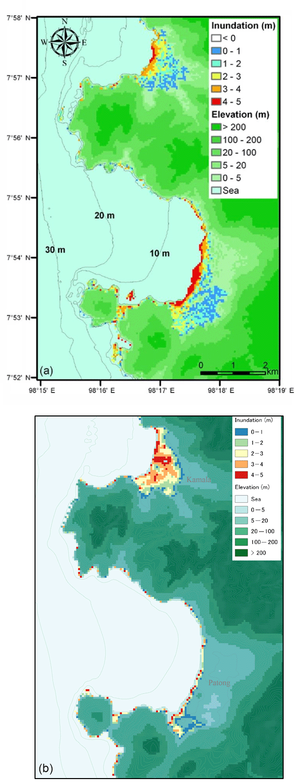
Figure 29 Kamala (north) and Patong (south) inundation maps comparison. (a) Inundation result by Supparsri et al. (2011). (b) TRITON-G inundation result.

Results for the second inundation validation in Phuket are compared with those of Supparsri et al. (2011). The wave arrival time for this region is of around 181 min, which agrees with the values obtained by TRITON-G model of 180 min. Inundation results are shown in Fig. 29, the image on top presents the inundation simulation obtained in the report while the image on the bottom depicts the results of TRITON-G model.

The results around the Kamala region coincide very well between models. Both report maximum inundation heights of around 5–6 m, and the run-up distances follow the same pattern. In the south, at Patong region however, there is a difference in the run-up distances. This is explained by the difference in the bathymetry used by TRITON-G. While in the Supparsri et al. (2011) study, a 52 m resolution was used on the entire inundation area, our model only used 50 m resolution bathymetry in Kamala. For Patong, values were interpolated from a lower 150 m resolution database, which produced a smoother topography and less accurate run-up results. This highlights the importance and the effect of having accurate and realistic bathymetry for the simulation.

This test, together with the good results obtained in the inundation benchmark comparisons (Sect. 6 and “Appendix”), served to validate the ability of TRITON-G to estimate tsunami inundation.

8 Conclusions

The tragic events of recent tsunamis showed the importance of developing fast and accurate forecasting models. We implemented several techniques to reduce the time to solution to meet our runtime goals in the successful development of this fast and accurate tsunami operational real-time model. In a short time, wide-area simulations (ocean size) can be obtained much faster than real time, meeting our goal for results in less than 15 minutes. The combination of highly accurate numerical methods with light stencils provided an excellent solution to the governing equations and gave stability on complex bathymetry. A customized, tree-based refinement that captured complex coastline shapes was successfully implemented using two factors; distance and focal areas. Using the distance from the coast to refine allowed us to leave coarser blocks in the open ocean, while blocks near the shoreline were refined to a higher 50 m resolution. Focal areas were also successfully introduced in the refinement to delimit the regions where the high-resolution blocks were generated and to use memory and computational resources efficiently. A full-GPU double-precision implementation was proven successful in delivering a large increase in speed. All parts of this simulation, including output storage are processed entirely on GPU with specialized kernels. For multi-GPU, the use of a weighted Hilbert space-filling curve successfully generate balanced domain partitions and workload.

Using Tsubame 3.0's GPU Tesla P100 cards for a full-scale simulation of 10 h resulted on a wall-clock time of just under 10 min with three GPU cards, including considerably sized output (65 GB) while using double precision. The hindcast of the Indonesian 2004 tsunami served to compare and validate TRITON-G simulation results, finding very good agreement with gauge propagation and inundations. Additionally, good agreement with standard inundation benchmark problems BP4, BP6, BP7 and BP9 was obtained. The flexibility and robustness of TRITON-G allows it to be an excellent operational model that can be easily adjusted for different tsunami scenarios, and its speed permits it to be a real-time forecasting tool. For these reasons, and under the collaboration with RIMES, TRITON-G has been successfully deployed as their operational model since August 2017.

Appendix A: Benchmark problem no. 4: solitary wave on a simple beach – laboratory

Numerical results for benchmarks 4, 6 and 7 are presented in this section. A detailed description of the problems can be found in NTHMP (2012). Here, we give a brief explanation in each section for completeness.

The domain for this test is shown in Fig. A1. In this problem, the wave height H is located at a distance L from the beach toe. This test was replicated in a wave tank 31.73 cm long, 60.96 cm deep and 39.97 cm wide at the California Institute of Technology. Several experiments with different water heights were performed. Benchmark problem 4 (BP4) uses the datasets for $H/d=\mathrm{0.0185}$ non-breaking wave and $H/d=\mathrm{0.30}$ breaking wave for code validation. Results use dimensionless units with the help of parameters like length d, velocity scale $U=\sqrt{gd}$ and time scale $T=\sqrt{d/g}$.

A1 Problem setup

The following parameters were used for the computation.

• Parameters: d=1 and g=9.8 in case A with $H/d=\mathrm{0.0185}$ and case B with $H/d=\mathrm{0.30}$.

• Friction: the Manning coefficient is set to 0.01.

• Computational domain: the domain along x direction spans from $x=-\mathrm{20}$ to x=80.

• Boundary conditions: a non-reflective boundary condition is used at the right side of the computational domain.

• Grid resolution: the numerical results presented are solved with a resolution of Δx=0.1.

• CFL: the value is set to 0.9.

• Initial condition: the initial wave is computed based on the following equations for height (η) and velocity (u).

  $$\begin{array}{}\text{(A1)}& {\displaystyle }& {\displaystyle }\mathit{\eta }\left(x.0\right)=H{\mathrm{sech}}^{\mathrm{2}}\left[\mathit{\gamma }\left(x-x_{\mathrm{s}}\right)/d\right]\text{(A2)}& {\displaystyle }& {\displaystyle }u(x,\mathrm{0})=-\mathit{\eta }(x,\mathrm{0})\sqrt{{\displaystyle \frac{g}{d}}}\end{array}$$

A1.1 Tasks to be performed

To accomplish this problem, the following tasks should be performed.

1. Compare the numerically calculated surface profiles at t$/T=\mathrm{30}:\mathrm{10}:\mathrm{70}$ for the non-breaking case $H/d=\mathrm{0.0185}$ with the lab data (case A).

2. Compare the numerically calculated surface profiles at $t/T=\mathrm{15}:\mathrm{5}:\mathrm{30}$ for the breaking case $H/d=\mathrm{0.30}$ with the lab data (case C).

3. Compute the maximum run-ups for at least one non-breaking and one breaking wave case.

A1.2 Numerical results

We present the numerical results obtained using TRITON-G. Figure A2 shows the comparison between water surface level measured in the experiment and the modeled numerical results obtained by our model for times 30, 40, 50, 60 and 70 for case A ($H/d=\mathrm{0.0185}$). Our results show good agreement between the numerical simulation and the non-breaking experiment.

Table A1 shows the errors computed for the NRMSD and for the maximum wave amplitude error (MAX). The error values obtained by the NTHMP workshop models are also included for comparison. These values are divided into two columns: one with results for the non-dispersive models (ND) and the other with results for the non-dispersive and dispersive models together (labeled ALL).

Errors obtained from our simulation tend to be similar or smaller than those errors obtained by other ND models, with just slight exception for time 70. Additionally, except for time 70 our errors are smaller than those obtained combining non-dispersive and dispersive mean error values.

Water level comparison for case C ($H/d=\mathrm{0.30}$) at times 15, 20, 25 and 30 is shown in Fig. A3. Table A2 gathers the values for NRMSD and MAX errors for our numerical results and for the NTHMP workshop models. In this case, only the results of models that reported their errors are included (taken from Tables 1–8, p. 41 in NTHMP, 2012).

For case C conditions, the shallow water equations are no longer appropriate for modeling and hydrostatic models tend to produce larger differences than non-hydrostatic ones. Our numerical results in general show good agreement with the experiment.

The difference with the steepening of the crest that is noticeable in the results is expected from a hydrostatic model. In spite of that, this steepening in our model is not very large and it can trace the wave front well. Once the wave breaking occurs, our model can simulate the run-up reasonably well. This is also partly reflected in the small NRMSD error estimation obtained by our model after the wave breaking.

Maximum run-up for case A and case C were calculated. For the non-breaking case A, the obtained run-up value is 0.091, and for the breaking case C, the run-up estimated is 0.588. These values are plotted in Fig. A4 with a yellow and red dot, respectively. It can be seen that both values lie well within the experimental results.

A2 Benchmark problem no. 6: solitary wave on a conical island – laboratory

The goal of this benchmark is to compare computed model results with laboratory measurements obtained during a physical modeling experiment conducted at the Coastal and Hydraulic Laboratory, Engineer Research and Development Center of the US Army Corps of Engineers. The laboratory's physical model was constructed as an idealized representation of Babi Island in the Flores Sea, Indonesia, to compare with Babi Island run-up measured shortly after the 12 December 1992 Flores Island tsunami (Yeh et al., 1994). Figure A5 show schematics of the experiment.

A2.1 Tasks to be performed

To accomplish this benchmark, the following values should be used.

• Case A: water depth d=32.0 cm, target H=0.05, measured H=0.045

• Case B: water depth d=32.0 cm, target H=0.20, measured H=0.096

• Case C: water depth d=32.0 cm, target H=0.05, measured H=0.181

Model simulations should then be conducted to address the following:

1. demonstrate that the two wave fronts split in front of the island and collide behind it;

2. compare the computed water levels with laboratory data at gauge 6, 9, 16 and 22;

3. compare the computed island run-up with laboratory gauge data.

A2.2 Problem setup

The following parameters were used for the computation.

• Computational domain: the dimensions are [$-\mathrm{5},\mathrm{23}]\times [\mathrm{0},\mathrm{28}]$;

• Boundary condition: open boundaries are used;

• Initial condition: the same solitary wave as proposed in BP4 with the correction for two dimensions;

• Grid resolution: the numerical results presented are solved with a resolution of Δx=0.05.

• CFL: the value is set to 0.9.

• Friction: the Manning coefficient is set to 0.02.

A2.3 Numerical results

We present the numerical results obtained using TRITON-G for the three cases (A–C) except for the splitting–colliding item. For this item, Fig. A6 shows the wave front splitting in front of the island and then colliding again behind it for case B (H=0.096); analog behavior was obtained for the other two cases.

Water level comparison uses values for gauges 6, 9, 16 and 22 for each of the three cases. Gauge 6 is located at (9.36, 13.80, 31.7), Gauge 9 is located at (10.36, 13.80, 8.2), Gauge 16 is located at (12.96, 11.22, 7.9) and Gauge 22 is located at (15.56, 13.80, 8.3).

Numerical results for cases A–C are shown in Figs. A7–A9, respectively. In the three cases, results were stable and in good agreement with the experimental values. The incident wave height and arrival time was captured for all gauges well. Similarly as with BP4, the steepening of the wave with increasing H is expected in a non-hydrodynamic model.

After the wave hit the island, some differences between the experimental and model wave were noticeable as the initial wave height increased. These oscillations in the experimental data represent the effects of dispersion, which our non-dispersive numerical method is not designed to capture. Despite this, the modeled waves show good agreement with the shape of the experimental waves, and the errors estimated tend to be small.

Table A3 gathers the normalized root-mean-square deviation (NRMSD) error and the maximum wave height (MAX) error. For comparison, mean errors obtained by the participating models in the NTHMP workshop are also included. These are separated in two columns, one for non-dispersive (ND) models and the other for non-disperse and disperse models together (ALL).

NRMSD errors for our model tend not to be very large and in similar range than those of the other non-dispersive models. In the case of the maximum height error (MAX), in almost all cases our model produced smaller error values than the non-dispersive model counterparts. Additionally, in most cases our MAX errors are smaller than those errors of the combined non-dispersive and dispersive mean values.

Figure A10 shows the comparisons between computed and experimental run-up around the island for the three cases. Case A represents the best agreement with the experimental values. Differences increased with steeper wave cases B and C, as several reflections and refraction possibly occur in the basin.

Table A4 gathers the errors obtained by our model and by the participating models in the NTHMP workshop for run-up cases A–C. Figure A10 showed the good agreement for case A, and this is also reflected in the NRMSD and MAX error results. Both values are considerably smaller than those errors obtained by the NTHMP non-dispersive (ND) models and by the non-dispersive and dispersive together (ALL). For cases B and C, the errors tend to be larger than but still similar to those obtained by other non-dispersive models. In all cases, the error stayed below the 20 % recommended criteria.

A3 Benchmark problem no. 7: the tsunami run-up onto a complex 3-D beach – laboratory

A laboratory experiment using a large-scale tank at the Central Research Institute for Electric Power Industry in Abiko, Japan, was focused on modeling the run-up of a long wave on a complex beach near the village of Monai (Liu et al., 2008). The beach in the tank was a 1 : 400-scale model of the bathymetry and topography around a very narrow gully, where extreme run-up was measured.

A3.1 Problem setup

The following parameters were used for the computation.

• Grid resolution: 393×244 was used with the same resolution 0.014 m as the bathymetry.

• CFL: the value is set to 0.9.

• Initial condition: is water at rest.

• Friction: the Manning coefficient is set to 0.01.

• Boundary conditions: solid wall boundaries were used at the top and bottom. At the left boundary, the given initial wave (shown in Fig. A11) was used to specify the condition up to time t=22.5 s. After that, it became a wall boundary condition.

A3.2 Tasks to be performed

To accomplish this benchmark, it is suggested to

1. model propagation of the incident and reflective wave accordingly to the benchmark-specified boundary condition;

2. compare the numerical and laboratory-measured water level dynamics at gauges 5, 7 and 9;

3. show snapshots of the numerically computed water level at the time synchronous with those of the video frames; and

4. compute the maximum run-up in the narrow valley.

A3.3 Numerical results

This section presents the numerical results for BP7 obtained with TRITON-G to achieve the required tasks.

The comparison with the three requested gauges 5, 7 and 9 is shown in Fig. A12 from t=0 to t=25 s. Good agreement is found between modeled and experimental wave for the three cases.

Values for the normalized root-mean-square deviation error (NRMSD) and maximum wave amplitude error (MAX) were estimated for the gauge results. For gauge 5, the NRMSD error is 10 % and MAX is 0.89 %. For gauge 7, NRMSD is 10 % and MAX is 4.81 %. For gauge 9, the NRMSD error is 6.57 % and MAX is 2.66 %.

Comparison with the extracted movie frames is shown in Fig. A13. In the left column are the five frames provided from the laboratory recording. These are frames 10, 25, 40, 55 and 70, extracted from the video with a 0.5 s interval. We found good agreement in time and space for times 15 to 17 s in 0.5 s increments, shown in the right column. The side-by-side comparison shows that the modeled wave follows the experimental wave front well. Additionally, the model captures the rapid run-up–rundown in the narrow gully.

Finally, the data provided by the benchmark workshop include a series of experiment tests for maximum run-up. Its maximum run-up is recorded at x=5.1575 and y=1.88 m with an average value of approximately 0.09 m. In comparison, our numerical result recorded a maximum run-up at around t=16.5 with a height of 0.0936 m at x=5.15 and y=1.88 m.

Table A1 Modeled surface profile errors with respect to laboratory experiments for case A $H/d=\mathrm{0.0185}$ at times 30, 40, 50, 60, and 70. Results from the NTHMP workshop errors are separated in non-dispersive (ND) models and all models (ALL).

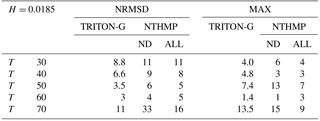
Table A2 Modeled surface profile errors with respect to laboratory experiments for case C $H/d=\mathrm{0.30}$ at times 15, 20, 25 and 30. Results from the NTHMP workshop model errors available are shown (ALL).

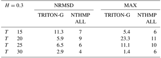
Table A3 Water level time series TRITON-G model errors with respect to laboratory experiment data for cases A–C. Mean values obtained for the performing NTHMP models are separated in non-dispersive models (ND) and non-dispersive and dispersive models together (ALL).

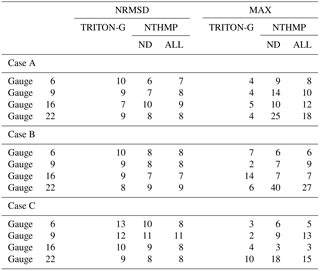
Table A4 Run-up TRITON-G model errors with respect to laboratory experiment data for cases A–C. Mean values obtained for the performing NTHMP models is separated in non-dispersive models (ND) and all models (ALL) and presented for better comparison.

Figure A1 Domain sketch for BP4, slope 1:19.85 (figure taken from benchmark description).

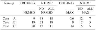
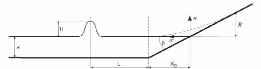
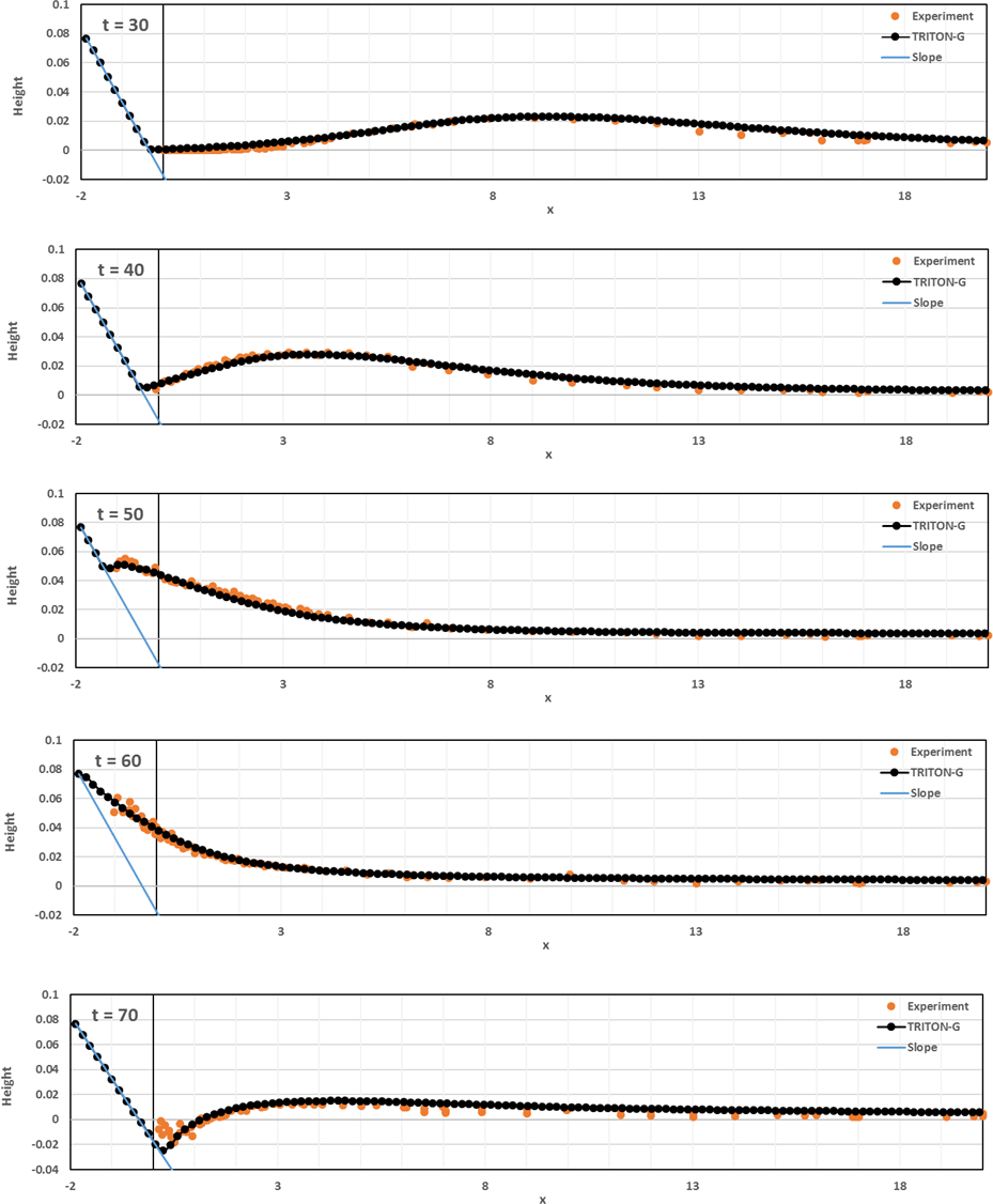
Figure A2 Comparison of numerically calculated free surface profile at different dimensionless times for the non-breaking case $H/d=\mathrm{0.0185}$.

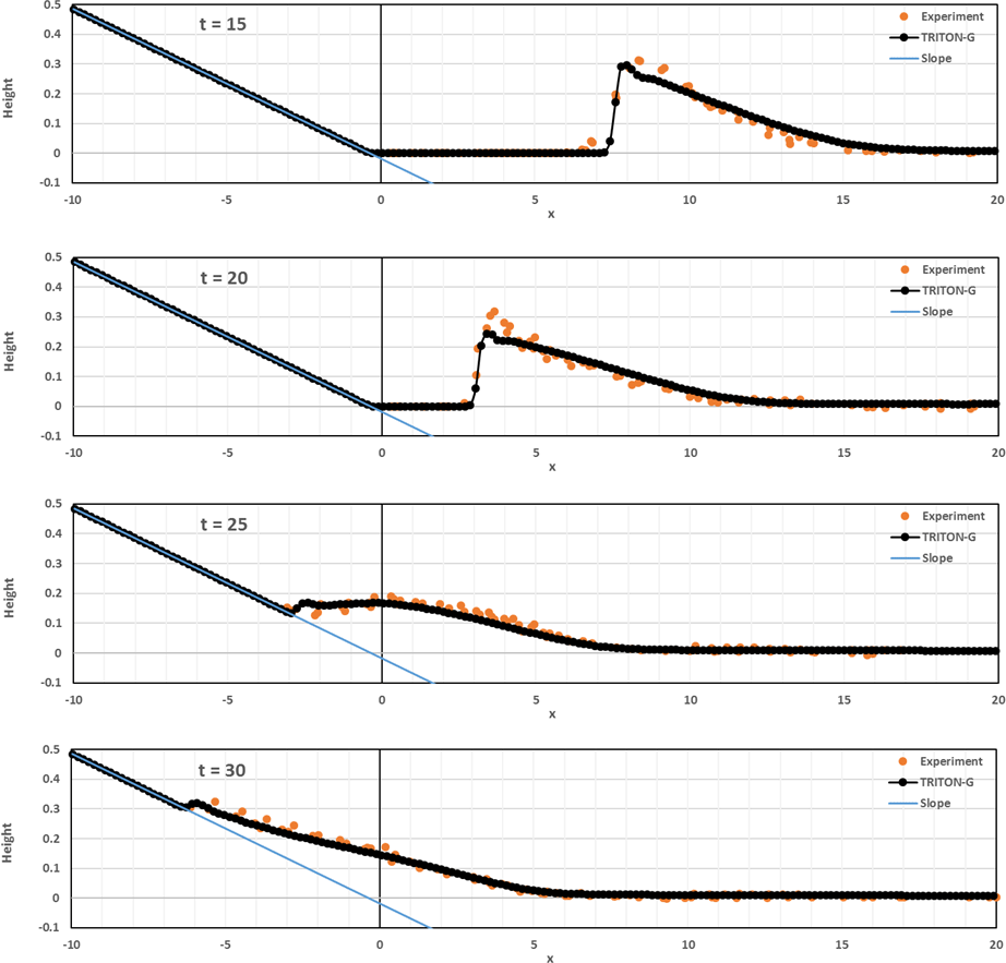
Figure A3 Comparison of numerically calculated free surface profile at different dimensionless times for the breaking case $H/d=\mathrm{0.30}$.

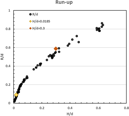
Figure A4 Scatter plot of non-dimensional maximum run-up from a total of more than 40 experiments conducted by Y. Joseph Zhan (Synolakis, 1987). The orange point indicates TRITON-G result for the breaking case $H/d=\mathrm{0.30}$, and the yellow point indicates the result for the non-breaking run-up case $H/d=\mathrm{0.0185}$.

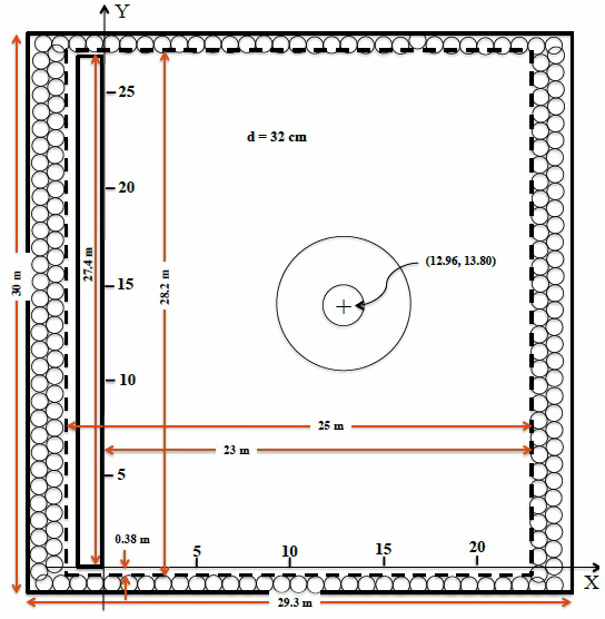
Figure A5 Basin geometry and coordinate system. Solid lines represent approximate basin and wavemaker surfaces. Circles along walls and dashed lines represent wave-absorbing material.

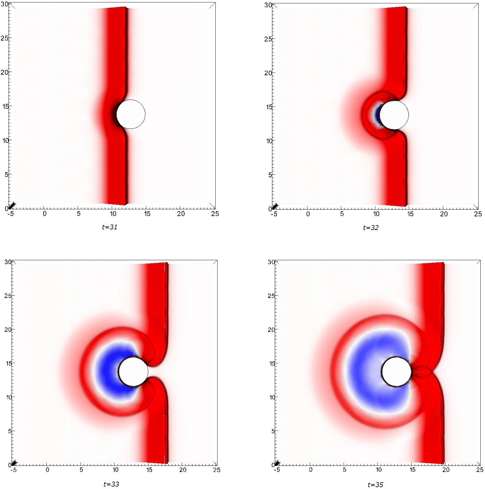
Figure A6 Snapshots at several times showing the wave front splitting in front of the island and colliding behind it for case B.

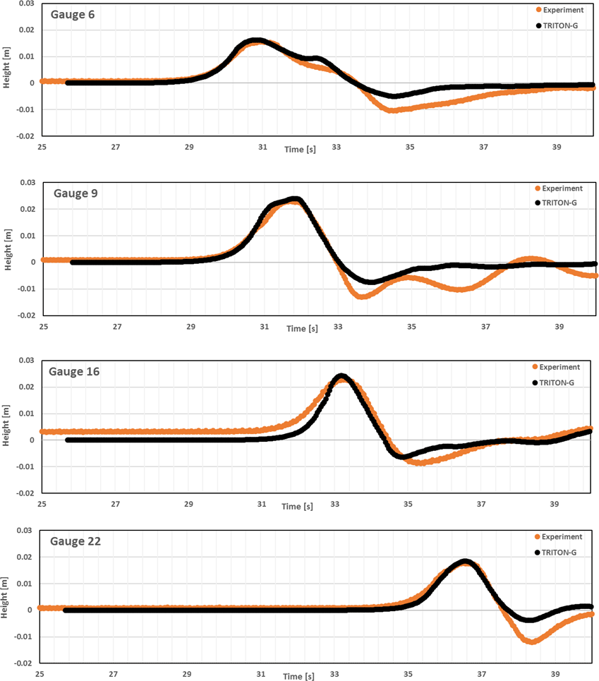
Figure A7 Comparison between computed and measured water levels at gauges 6, 9, 16 and 22 for case A (H=0.045).

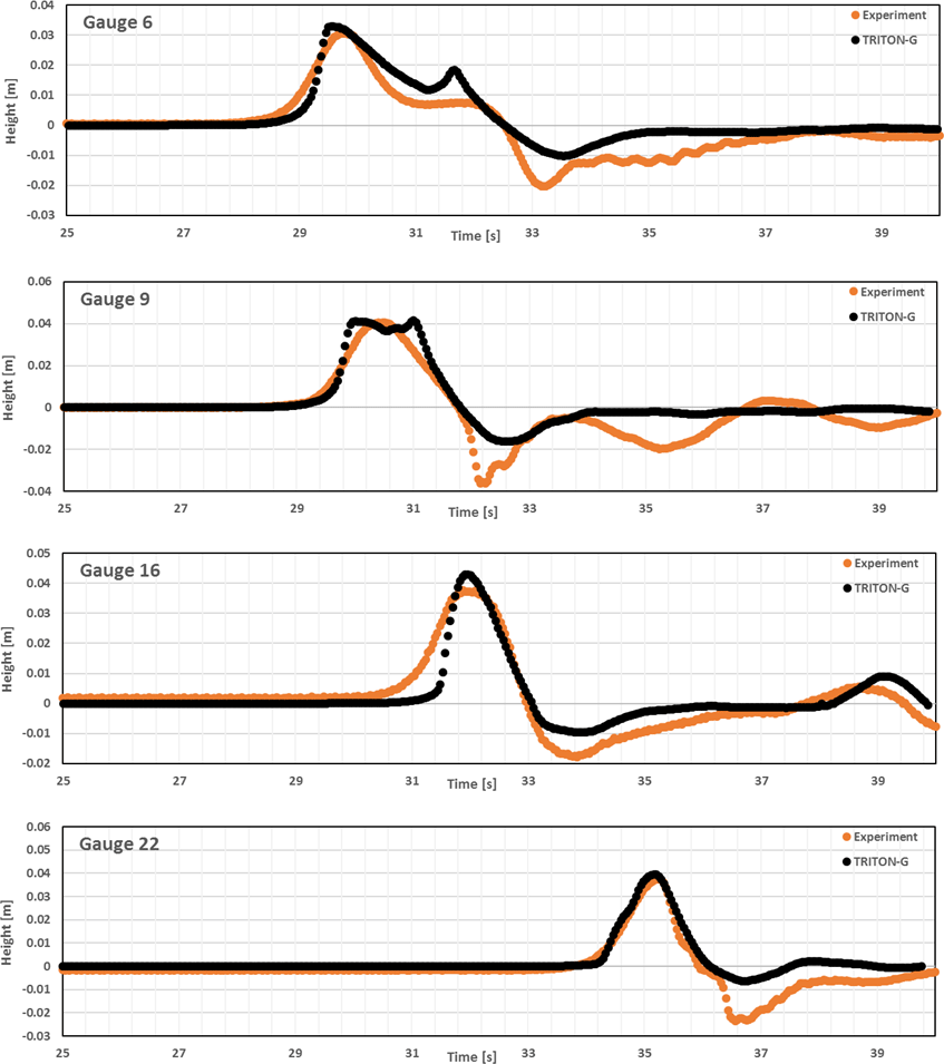
Figure A8 Comparison between computed and measured water levels at gauges 6, 9, 16 and 22 for case B (H=0.096).

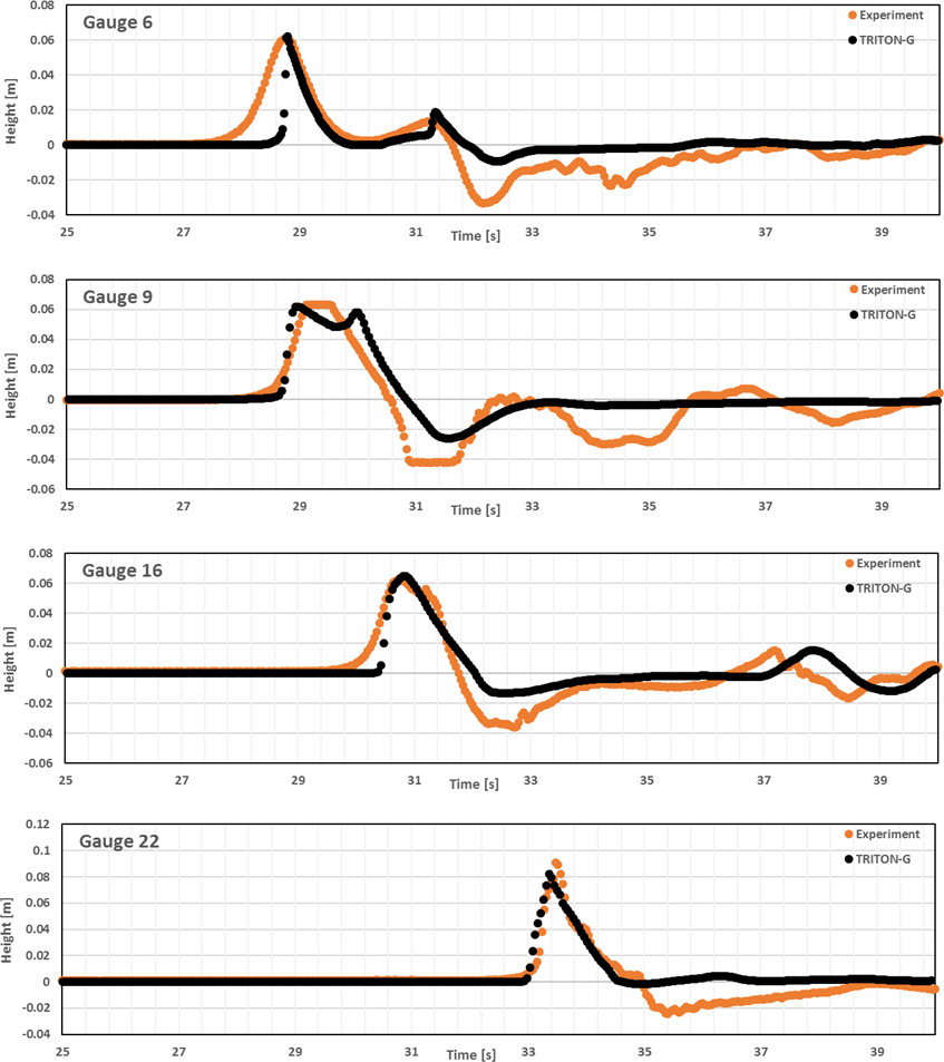
Figure A9 Comparison between computed and measured water levels at gauges 6, 9, 16 and 22 for case C (H=0.181).

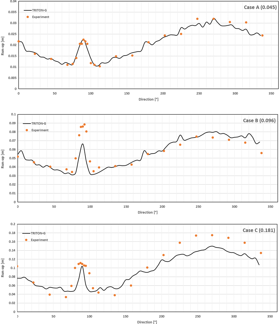
Figure A10 Comparison between computed and measured run-up around the island for the three cases.

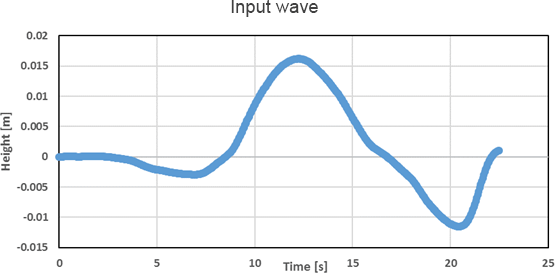
Figure A11 Prescribed input wave for the left boundary condition, defined from t=0 to t=22.5 s.

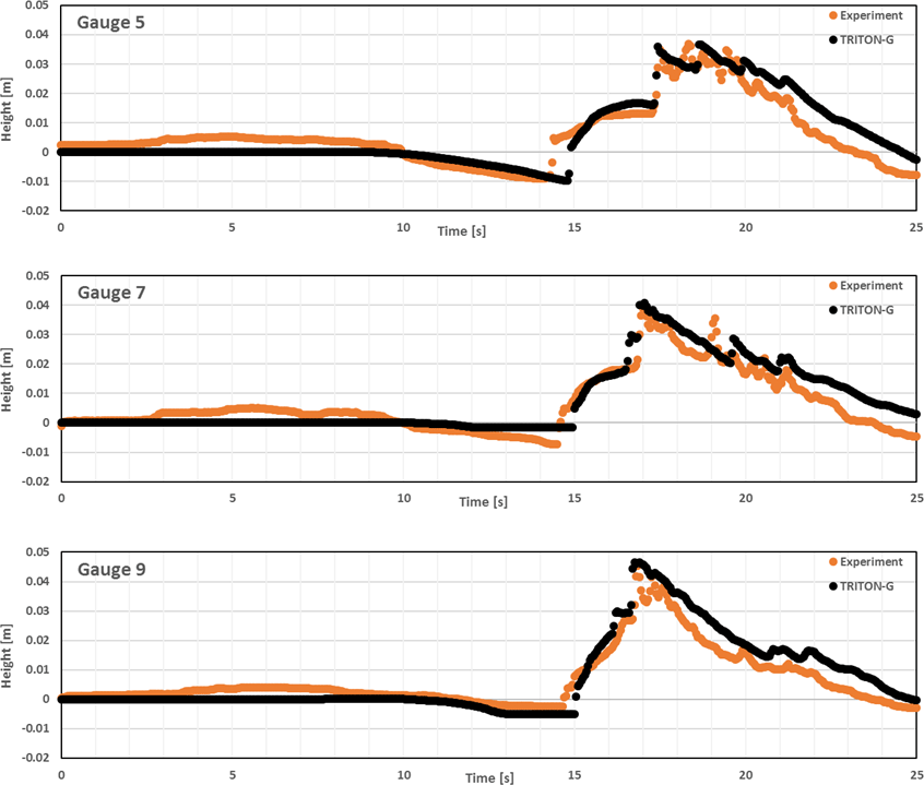
Figure A12 Water level comparison for BP7 between experiment and TRITON-G for gauges 5, 7 and 9.

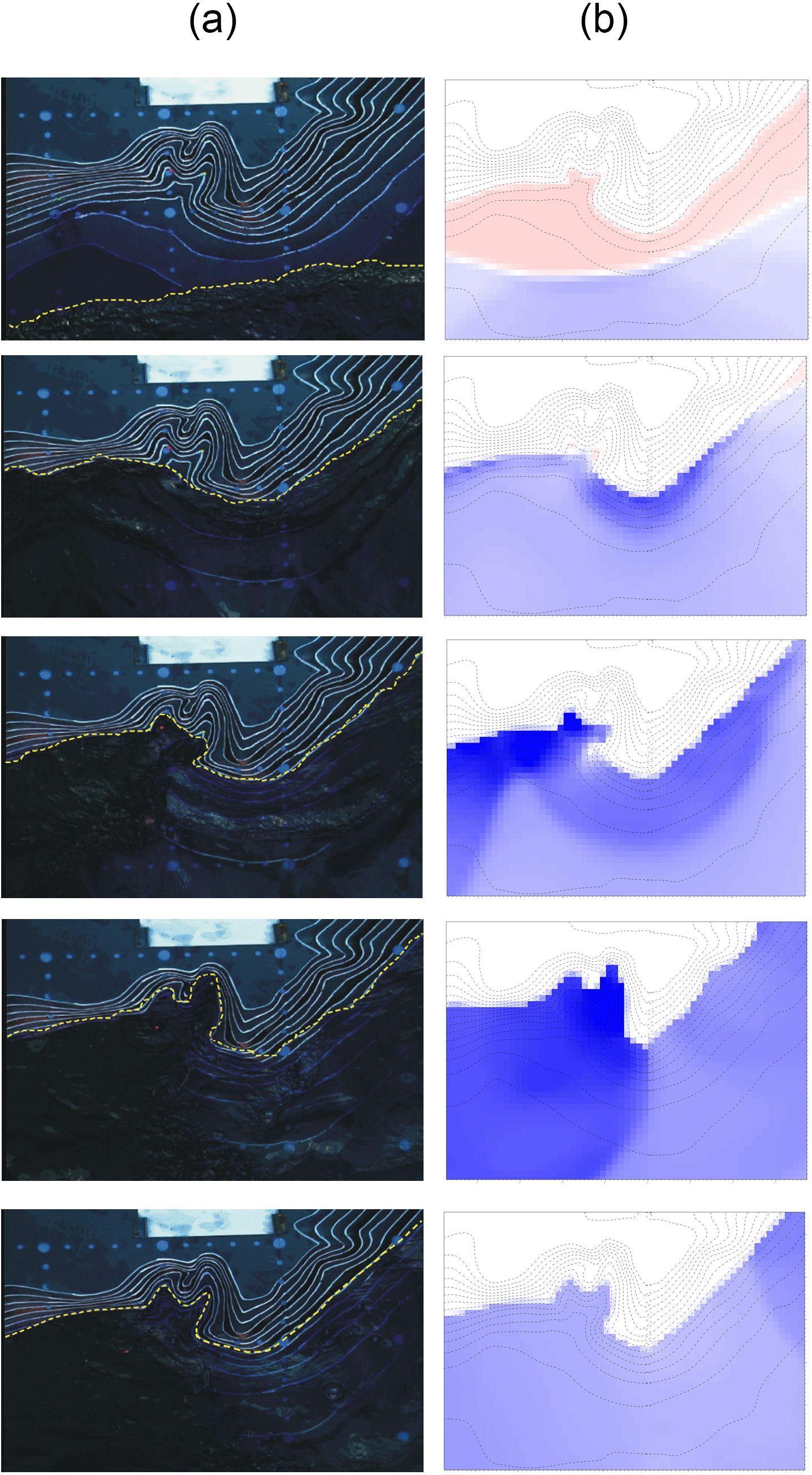
Figure A13 Comparison between extracted movie frames (a) and TRITON-G simulation (b) for times 15, 15.5, 16, 16.5 and 17 s.