the Creative Commons Attribution 4.0 License.
the Creative Commons Attribution 4.0 License.
 | 19 Sep 2018
Assessing fragility of a reinforced concrete element to snow avalanches using a non-linear dynamic mass-spring model
Philomène Favier
David Bertrand
Nicolas Eckert
Isabelle Ousset
Mohamed Naaim
This paper presents an assessment of the fragility of a reinforced concrete (RC) element subjected to avalanche loads, and more generally to dynamic pressure fields applied orthogonally to a wall, within a reliability framework. In order to obtain accurate numerical results with supportable computation times, a light and efficient Single-Degree-of-Freedom (SDOF) model describing the mechanical response of the RC element is proposed. The model represents its dynamic mechanical response up to failure. Material non-linearity is taken into account by a moment–curvature approach, which describes the overall bending response. The SDOF model is validated under quasi-static and dynamic loading conditions by comparing its results to alternative approaches based on finite element analysis and the yield line theory. Following this, the deterministic SDOF model is embedded within a reliability framework to evaluate the failure probability as a function of the maximal avalanche pressure reached during the loading. Several reliability methods are implemented and compared, suggesting that non-parametric methods provide significant results at a moderate level of computational burden. The sensitivity to material properties, such as tensile and compressive strengths, steel reinforcement ratio, and wall geometry is investigated. The effect of the avalanche loading rate is also underlined and discussed. Finally, the obtained fragility curves are compared with respect to the few proposals available in the snow avalanche engineering field. This approach is systematic and will prove useful in refining formal and practical risk assessments. It could be applied to other similar natural hazards, which induce dynamic pressure fields onto the element at risk (e.g., mudflows, floods) and where potential inertial effects are expected and for which fragility curves are also lacking.
- Article
(3773 KB) - Full-text XML
- BibTeX
- EndNote


The hazard posed by avalanches threatens human communities in mountainous areas. Fatalities due to snow avalanches result from the practice of mountaineering or from avalanches reaching dwellings (e.g., an avalanche in 1999 killed 12 people in their homes in French Chamonix-Montroc village) or holiday accommodations (e.g., an avalanche in Val-d'Isère French valley in 1970 destroyed a vacation resort, where 39 people died; an avalanche in 2017 in the Italian Abruzzo region affected a hotel killing 29 people inside the buildings).
For formal risk assessment, fragility and/or vulnerability curves are required to evaluate individual risks (Keylock et al., 1999; Cappabianca et al., 2008; Eckert et al., 2012) or design defense structures by loss minimization (Eckert et al., 2008, 2009; Favier et al., 2016). For a given element at risk, the vulnerability relations represent its loss distributions, whereas the fragility curves represent its damage states distributions. Until now, very few fragility curves have been established for snow avalanches. Indeed, most studies have been dedicated to vulnerability curves (Papathoma-Köhle et al., 2011). Existing vulnerability and fragility relations were mostly empirically assessed, based on historical observations (Wilhelm, 1998; Keylock and Barbolini, 2001; Barbolini et al., 2004). Since these relationships were deduced from scarce data, which can be site-dependent, their accuracy and representativeness is questionable. Recently, in order to offer an alternative way of deriving vulnerability curves, finite element analysis (FEA) has been used to describe the damage level of typical reinforced concrete (RC) structures subjected to an avalanche pressure field (Bertrand et al., 2010). The main advantage of numerical approaches is that they accurately define and simulate the studied structure, e.g., through its geometry, the specificity of its technology and the non linear mechanical behavior of its materials. Using such numerical approaches, snow avalanche fragility curves have recently been proposed (Favier et al., 2014; Ousset et al., 2016).
In earthquake engineering, fragility curves have been widely studied and methodologies to determine these have traditionally been categorized as empirical, numerical, judgmental, or hybrid (Rossetto and Elnashai, 2003). For instance, for buildings exposed to earthquakes, the probability of overpassing a drift limit according to the peak ground acceleration is described via reliability-based numerical fragility curves (Ellingwood, 2001; Kyung and Rosowsky, 2006; Li and Ellingwood, 2007; Lagaros, 2008). On the contrary, for mass flow gravity-driven hazards, few fragility relationships have been developed. Indeed, the prevailing lack of documented fragility relationships in snow avalanche engineering can also be noticed in rockfall (Mavrouli and Corominas, 2010a, b) or landslide (Papathoma-Köhle et al., 2012) engineering.
Numerical fragility curves are mainly derived using the well-established framework of reliability analysis (e.g., Lemaire, 2005). Once the deterministic model and the failure criterion of the system are chosen, the uncertainties related to the random variables are propagated through the mechanical model in order to calculate the failure probability. Usually, simulation methods which give robust results are used, e.g., the direct Monte Carlo approach. However, they can be time consuming. If too many runs are needed to achieve an accurate estimate of the failure probability or if the deterministic model is not effective enough in terms of computation time, alternative sampling methods can be used, e.g., importance sampling (Melchers, 1989), subset sampling (Au and Beck, 2001). Such approaches do not always ensure the convergence of the results according to the non-linearity degree of the deterministic model or to the number of random variables involved.
In reliability analysis, very time-consuming models are generally discarded in favor of time-effective ones. Such alternative models, also called meta-models, are often built on a statistical basis, e.g., using polynomial chaos expansion (Sudret and Mai, 2013; Ousset et al., 2016) or, sometimes, on a physical basis. Simplifying assumptions on the mechanical model can be an efficient way to reduce computation times along with keeping the essential physics involved. This is especially true for reinforced concrete for which various numerical models exist to describe the mechanical response of a structure and its possible failure. Hence, in order to find a compromise between time-efficient but simplified models and refined but time consuming models, RC structures can be described using Single-Degree-of-Freedom (SDOF) models (Biggs, 1964), where the structure is modeled by an equivalent mass and an equivalent spring. This approach has been largely used and validated in the field of structures subjected to blast loads (Ngo et al., 2007; Jones et al., 2009; Carta and Stochino, 2013). On the contrary, in the field of snow avalanches such approaches are only emerging. A recent example is the application of a SDOF model to study the behavior of trees towards powder snow avalanche air blasts (Bartelt et al., 2018). As a consequence, the dichotomy remains quite strong between FEA approaches (Berthet-Rambaud, 2004; Bertrand et al., 2010; Ousset et al., 2013) and simpler models based of civil engineering abacuses (Favier et al., 2014), that is to say, models that use structural sizing tables to calculate the resistance of standard structures. The first allows a better understanding of the detailed interaction between avalanche flows and structures but only under very specific conditions due to the computational burden. The second allows obtaining the failure probability of an RC member impacted by snow avalanches for a wide range of boundary conditions. However, simplified approaches often operate under questionable assumptions (e.g., quasi-static response of the structure, no spatial pressure field distribution) and can lead to ignoring potential inertial effects due to the dynamic nature of the loading.
As a response to the important issue of obtaining accurate numerical results with reasonable computation times, this paper presents a light and efficient SDOF model and uses it to refine the assessment of physical fragility regarding snow avalanches to elements at risk, such as residential RC buildings. Even if several kinds of constructive technologies are used in snow avalanche engineering (e.g., masonry, reinforced concrete, or metallic structures), for the sake of simplicity only the most common type of structure found in avalanche prone areas in the Alps is considered: reinforced concrete. In order to justify the assumptions made for the avalanche loading, Sect. 2 reminds some of the main features of an avalanche and especially in terms of pressure magnitude that can be expected. Section 3 describes the proposed SDOF model used as a physically based meta-model of a more comprehensive finite element model of an RC wall subjected to the avalanche pressure. Based on FEA and limit analysis (yield line theory) comparisons, the SDOF model is able to describe the dynamic mechanical response of the RC wall up to its collapse by excessive bending. Section 4 exposes the statistical framework used to derive fragility curves using different sets of input variables and different reliability methods. Section 5 details the results, namely the relative efficiency of the different reliability methods tested, the sensitivity to input statistical distributions and geometric properties of the wall, and the influence of the loading rate on fragility curves. Section 6 discusses the curves obtained with respect to the crude proposals that can be found in the snow avalanche literature, highlighting the usefulness of the proposed approach for improving risk assessment. Finally, Sect. 7 highlights some key perspectives and conclusions.
Avalanches can be defined as the release of a snow volume that propagates down a slope under the action of gravity. Snow avalanches can be classified according to several criteria (e.g., snow type, release zone, weather conditions). Two main types of avalanches are distinguished: (i) powder snow avalanches composed of diluted dry snow, due to air incorporation, characterized by a mean flow velocity that can reach 100 m s−1 and having a density from 1 to 10 kg m−3; (ii) dense snow avalanches mostly composed of humid snow that can develop a mean flow velocity of hardly 30 m s−1 and a high density up to 500 kg m−3. The pressure field developed by an avalanche onto an obstacle depends on those latter features. Within the heart of the flow, high peak pressures can develop. For powder avalanches, important pressure values are related to high velocities of the flow and for dense snow avalanches to high snow densities.
Up to now, measured peak pressures span from 6.6 kPa at the Lautaret experimental site (Berthet-Rambaud et al., 2008) up to more than 1200 kPa at the Sionne site (Sovilla et al., 2008). However, this last pressure was measured very locally on the height of the avalanche front. The analysis of the signals data held by the authors suggests that the lowest recorded average loading rate is 6 kPa s−1 for a peak pressure of 21 kPa at the Lautaret experimental site (Thibert and Baroudi, 2010) and the highest is 400 kPa s−1 for a peak pressure of 490 kPa at the Taconnaz site (Bellot et al., 2013). Those measurements were made with sensors placed at key positions within the flow, typically in the middle of the avalanche path, where high pressures and high loading rates can be recorded (see for instance Schaerer and Salway, 1980; Berthet-Rambaud et al., 2008; Sovilla et al., 2008, 2013 or Thibert et al., 2015).
However, it must be stressed that such direct measurements, related back calculations, and numerical calculations of avalanches' pressure impacts and loading rates still suffer from large uncertainties and lack of information. In addition, dwellings and buildings are commonly located at the bottom of avalanche paths, in the so-called avalanche runout areas, where magnitudes of peak pressures and loading rates are lower than those recorded in the middle of avalanche paths, which adds further uncertainty to the analysis. This means that engineering studies, as with this study, cannot currently rely on very specific inputs to specify impact pressures and loading rate values. Hence, in most of what follows, because the RC wall is supposed to be located within the runout zone of the avalanche, a rough loading rate value of 0.1 kPa s−1 has been assumed. This leads to load the RC wall under quasi-static conditions. However, a specific section (Sect. 5.3.3) is dedicated to assessing the effect of the avalanche loading rate on the fragility curve derivation. In many European countries, if a building is located in an avalanche prone area, civil engineering standards impose that the wall facing the avalanche flow has to support pressures of up to 30 kPa.
In order to perform the fragility analysis of an RC wall impacted by an avalanche, the pressure field should be described in time and space. For the sake of simplicity, based on previous research, it seems reasonable to use the following assumptions for the modeling of the avalanche loading. A uniform spatial distribution of the pressure field (Fig. 1a) is used. It evolves through time with a triangular shape (Fig. 1b). One can note that in this paper, the assumption related to the temporal pressure field description can be easily changed if one wants to consider different pressure signals.
3.1 RC wall description
3.1.1 Geometry, loading, and material behavior laws

Figure 1 Simply supported RC wall loaded by a uniform pressure field (a) and time evolution of the applied pressure based on triangular shape (b). The maximal pressure (pmax) is reached for time where tend corresponds to the end of the pressure application.
We consider a simply supported wall with length L=8 m, width b=1 m, and thickness h=20 cm (Fig. 1a). The RC wall is simply supported along its two smaller edges and, thus, the problem can be described in 2-D. It is assumed that the snow avalanche applies a uniform pressure field p(t) along the y axis, which evolves through time from t=0 s to tend. The maximal pressure pmax is reached at time tend∕2 (Fig. 1b). The loading rate is defined as .
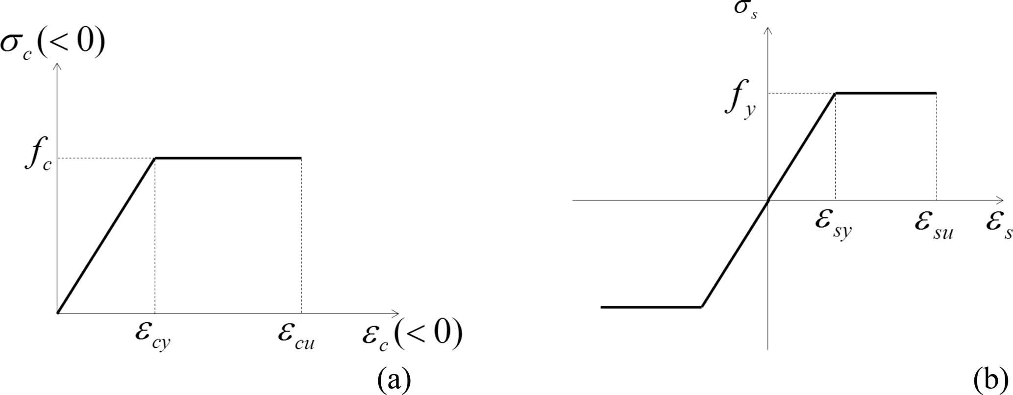
The concrete and steel behavior laws are described by piece-wise linear relationships that describe the evolution of stress σ as a function of strain ϵ. The elastic part of the behavior laws is described by the Young moduli of steel Es and concrete Ec.
Under compression regime, the stress σc increases linearly as a function of the strain ϵc up to the compressive strength of the concrete fc, which corresponds to a strain of ϵcy (Fig. 2a). Then σc reaches a plateau until the total crushing of the concrete under the ultimate compressive strain, where ϵc=ϵcu. In addition, it has been assumed that no tensile stress can develop within the concrete.
For steel, the behavior law is assumed to be elastic perfectly plastic (Fig. 2b). Variable fy is defined as the yielding stress related to the yielding strain ϵsy with fy=Esϵsy and ϵsu is the ultimate strain of steel. The reinforcement ratio of the RC wall, ρr, equals 0.4%. The latter is defined as the ratio between the steel area, As, and the cross-section area, . Figure 3a depicts a view of the cross section of the RC wall. Figure 3b–c depict the stress and strain diagrams.
3.2 SDOF model
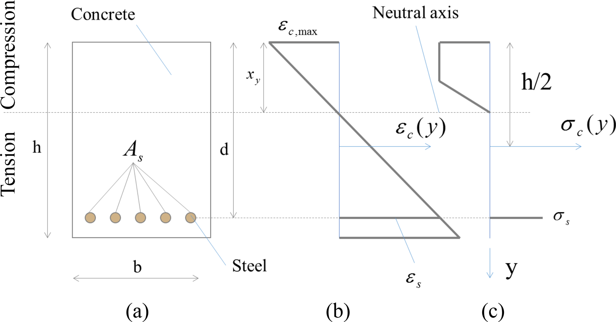
Figure 3 Cross-section of the RC beam (a), stress (b), and strain (c) distributions along y axis.

Figure 4 Simply supported beam (a), mass-spring system (b), and failure mode of the RC wall (c).
The SDOF model corresponds to a dynamic mass-spring system loaded by a force time evolution deduced from the uniform pressure field applied to the RC wall (Fig. 4a–b). An equivalent mass Meq is connected to a spring of equivalent stiffness Keq (Biggs, 1964). The expressions of Meq and Keq are deduced from the geometric features of the RC wall (geometry and boundary conditions) and from the mechanical properties of the RC material via bending moment–curvature relationship (M−χ relationship), respectively. In addition, no damping has been considered. If the structure collapses, the failure will occur during the loading phase and thus it is not necessary to account for the post-peak oscillation regime.
The loading rate (e.g., from 0.1 to 6 kPa s−1) involves higher characteristic times (e.g., about 1 to 20 s) than the first natural frequency of the structure with oscillation period of 0.2 s. Moreover, the slenderness of the RC wall is . Thus, it is possible to assume that the failure mode occurs due to the excessive bending moment at the midspan (Fig. 4c).
3.2.1 Elasto-plastic response
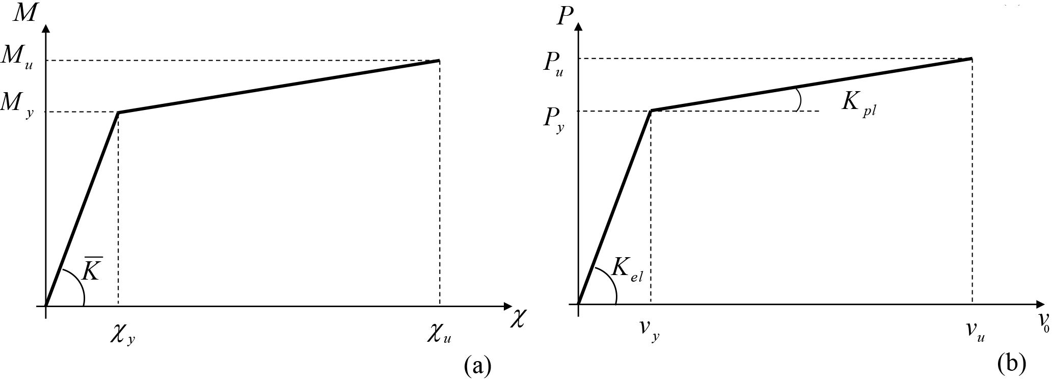
Figure 5 Bending moment–curvature relation (a) and load–displacement relation of the SDOF model (b).
The characteristic load–displacement curve (P−v0) of the RC wall is derived from the moment–curvature relationship (Fig. 5a) deduced at the cross-section scale (cf. Sect. 3.2.2). The bending moment (My) corresponds to the beginning of either steel yielding or concrete crushing depending on the reinforcement ratio. The ultimate bending moment (Mu) corresponds to the achievement of the ultimate strain value by either concrete or steel. The related curvature to My and Mu is χy and χu, respectively.
The P−v0 curve represents the elasto-plastic behavior of the SDOF model (Fig. 5b). The first part of the load–displacement bilinear curve represents the elastic response while the second part represents the plastic response of the RC wall. Forces are expressed as and , which can be transformed into a uniform pressure as (Fig. 4a). Then, the expression of the midspan displacement corresponding to the transition from elastic to plastic is
where is the bending stiffness of the RC wall. The ultimate midspan displacement is deduced from
where lp is the plastic hinge length (Fig. 4c), which can be estimated by the relation (Mattock, 1967), where d is the effective depth of the cross-section (Fig. 3a). Finally, the load–displacement curve (Fig. 5b) has two stiffnesses, which are defined as
3.2.2 Moment–curvature relationship
The curvature is defined as , where vo is the midspan displacement. The curvature is obtained assuming that the strain distribution along the y axis follows classical Euler–Bernoulli assumptions, meaning that the sections remain plane and orthogonal to the neutral axis during the loading of the RC wall (Fig. 3b). Thus, the curvature can be calculated as
where xy is the neutral axis depth. The value of xy is deduced from the translational mechanical balance along y of the cross-section, which can be expressed by
The moment–curvature relationship is constructed step by step by calculating the position of the neutral axis for a given strain distribution, i.e., a given curvature χ, which fulfills the condition of Eq. (6). Next, the bending moment is calculated from
At the end of the process, My, Mu, χy, and χu are identified on the M−χ curve and used to derive the load–displacement curve of the SDOF model.
3.2.3 Equations of motion
From Newton's second law, the dynamic mechanical balance of the SDOF produces the following ordinary differential equations. For the elastic phase, where :
and, for the plastic phase, where ,
where , Mel and Mpl are elastic and plastic equivalent masses, respectively, which are calculated as and with Mtot the total mass of the beam, and and (Biggs, 1964), P(t) is the time evolution of the external force deduced from the uniform pressure p(t) applied to the RC wall. In order to solve Eqs. (8) and (9) over time, the usual Newmark's algorithm techniques were used (Newmark, 1959).
If needed, non-uniform spatial distributions of the pressure field can be described by the SDOF model (Biggs, 1964). In that case, the pressure (p(x, t)) depends on the time (t) but also on the position (x) onto the RC wall. It is assumed that the spatial distribution of the pressure field remains the same during the entire simulation. Only its magnitude evolves. The transformation factors are established from and , where , m is the mass of the beam per unit length and ϕ(x) describes the qualitative shape of the structure taken to be the same than the one resulting from the static loading application under the external load p(x).
3.3 Validation
3.3.1 Finite element analysis
To validate the SDOF model, a finite element simulation of the RC wall response to an avalanche load was undertaken using the computation software Cast3M (Millard, 1993). The analysis was carried out in 2-D and the RC wall is assumed to behave as a simply supported beam. Multi-fiber beam finite elements were used. The formulation of these finite elements is based on classical assumptions of Euler–Bernoulli. Concrete and steel were distributed over the cross section of the beam via fibers (Fig. 6), where the uniaxial response of both materials are described along the longitudinal x axis. The same behavior laws (Fig. 2) have been used within the finite element analysis. A total of 100 finite elements were placed along the x axis and 7 along the y axis. A perfect adhesion between concrete and steel was assumed. A uniform pressure was applied along y axis over the total length L of the beam.
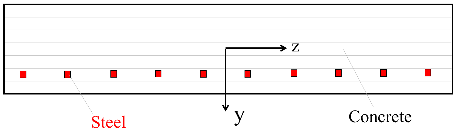
Figure 6 Cross section discretization of the beam multi fiber finite element. The diameter sizes of the steel reinforcements are knowingly exaggerated.
3.3.2 Limit analysis (yield line theory)
Under quasi-static loading conditions, the ultimate resistance of RC slabs under uniformly distributed pressure can be derived from classical yield line theory (Johansen, 1962), which also provides the collapse mechanism of the RC wall. Under external loading, macro-cracks will develop to form a pattern of yield lines until a mechanism is formed and total collapse takes place. A yield line corresponds to a nearly straight line along which a plastic hinge develops, where the bending moment becomes constant and equals the plastic bending moment. The ultimate pressure is deduced from the energy balance between external and internal energies. The external energy coming from the loading and the internal energy is due to energy dissipation within the yield lines.
For a simply supported one-way slab, the only collapse mechanism that can arise is depicted in Fig. 4c. Under uniform pressure, a single yield line would develop at the mid span and thus, for a given arbitrary midspan rotation θ, the internal work, calculated as 2θMp, equals the external work, calculated as . Finally, it leads to the ultimate pressure , where Mp is the plastic bending moment of the RC wall. The value of Mp can be obtained by (Favre et al., 1990)
which leads to Mp=57.6 kN m and finally qYLT=7.2 kN m−2.
3.3.3 Results comparison
Figure 7 Comparisons of (a) FEA (CASTEM), SDOF models, and ultimate load prediction by yield lines theory in the case of a quasi-static pushover test; and (b) time evolution of the mid-span displacement (v0) of the RC wall for several loading times () (blue: 0.1, cyan: 0.2, red: 0.3, black: 0.5, magenta: 1, green: 2, yellow: 5 s).
Table 1 summarizes the inputs of the FEA and the SDOF models. Table 2 gives a comparison of ultimate displacement, ultimate pressure, and computation time. With the same computer, a computation time of 5 min is needed for the FEA whereas the SDOF model runs and finishes calculations in nearly 10 s. Limit analysis is time efficient but only provides the ultimate pressure.
Results demonstrated that both models are in very good agreement under either quasi-static (Fig. 7a) or dynamic conditions (Fig. 7b). In the first case, the elastic regime is accurately described by the SDOF model. The ultimate pressure is also well-reproduced, even if a slight underestimation can be noted due to the estimation of the ultimate bending moment (Mp) from the approach of Favre et al. (1990). Moreover, a slight difference can be noticed concerning the ultimate displacement, which is higher in the case of the FEA. This can be explained by the formulation of the beam fiber element, where the tangent stiffness matrix approaches zero when the structure is close to the collapse. Within a reliability context, those observations ensure the SDOF model is able to provide conservative and hence safe results for the ultimate state prediction of the RC wall. Under dynamic loading conditions, the FEA and the SDOF models develop a very similar response over time (Fig. 7b) for a width range of loading times.
Table 1Parameter values for models comparison. The following notations are adopted: Ult. is an abbreviation of ultimate, S signifies steel, and C signifies concrete.
Table 2Ultimate displacement, ultimate pressure and computation time provided by the three approaches considering quasi-static pushover test.
4.1 Failure probability definition
The quantification of failure probability is carried out through the reliability analysis of the physical model (Lemaire, 2005). Thus, the deterministic model (i.e., physical model) is combined with the probabilistic description of the model inputs and with an ad hoc reliability method used to compute the failure probability of the structure. The assessment of the random response of the system is expressed by the probability density function fR(r), where R is the structure resistance. The related cumulative distribution function is obtained by integration and gives the failure probability for a given solicitation s which is, in this case, the maximal pressure applied to the wall over time. The failure probability is expressed as
where the capacity r of the RC wall is defined by its ultimate state which is directly related to the ultimate displacement. Thus, the failure criteria is defined as , where vmax is the maximal displacement of the RC wall through time, i.e., . The case where g≤0 corresponds to the RC wall collapse. The fragility curve is obtained by calculating the cumulative distribution function curve defined as . In the following, the probability distributions of the physical model inputs (i.e., geometry and material properties) are presented and, then, the reliability numerical methods used to derive fragility curves are shown.
4.2 Inputs probability distributions
Two classes of inputs are considered random variables, i.e., geometrical (L, b and h) and strength-related (fc, fy and ρr) variables. In addition, several sets of input variable distributions are used, depending on (i) the values of the coefficients of variation (from 0, the deterministic case, to 0.18); (ii) the choice of the probability distributions expression; and (iii) independent or dependent distributions. These are summed up in Table 3.
Table 3Marginal distributions of input parameters. “determ.” means deterministic, which corresponds to a coefficient of variation (COV) equal to zero. In the case of independent variables, normal distributions are used (* mean of fy is 560 MPa for set J).
4.2.1 Independent probability distribution function distributions
To describe geometrical uncertainties, normal distributions are largely assumed (Lu et al., 1994; Val et al., 1997; Low and Hao, 2002; Kassem et al., 2013). The coefficient of variation (COV) is usually taken from a range of 0.01 to 0.05. Three sets (1, 2, 3 of Table 3) of COV are tested using normal distributions.
Regarding both compressive and tensile strength parameters, in a first approximation, normal distributions with a COV of 0.05 are considered (set a). Second, more realistic COV are used (set b). For the compressive strength of concrete fc the normal distribution is the usual choice (Mirza et al., 1979; Val et al., 1997; Low and Hao, 2001, 2002) and a COV ranging from 0.11 to 0.18 is generally used. Here a COV of 0.18 is used (set b). Finally, for the tensile steel parameter fy, normal, log-normal, or beta distributions are often proposed (MacGregor et al., 1983) and the COV varies from 0.08 to 0.11 (Val et al., 1997). In the paper, a normal distribution is adopted and the COV equals 0.08 (set b).
No data is available regarding the reinforcement ratio's COV. As ρr is defined from geometrical parameters, a normal probability distribution function (PDF) is assumed and the COV is assumed to be equal to 0.05, 0.03 and 0, for sets α, β, and γ, respectively.
4.2.2 Strength parameters advanced expression

Figure 8 Statistical distributions of (a) the concrete compressive strength fc and (b) the normally distributed steel yield strength fy according to Table 3.
The JCSS (Joint Committee on Structural Safety, JCSS, 2001) proposed more realistic distribution descriptions by accounting for their potential dependencies (cf. set J, Table 3). The distribution of fc is deduced from the basic concrete compression strength fc28 distribution. For a ready-mixed type of concrete with a C25 concrete grade, it yields:
where the values of the parameters are: m=3.65, v=3.0, s=0.12, n=10 and, tv is a random variable from a Student distribution with v degrees of freedom. Then, fc is calculated as follows:
where λ is assumed to be equal to 0.96 and accounts for the systematic variation of in situ compressive strength and the strength from standard tests, αc equals 0.92, and Y1 is a log-normal variable representing additional variations due to the special placing, curing, and hardening of the concrete with a mean of 1 and coefficient of variation 0.06.
For the yield strength of steel (fy) based on JCSS assumptions, a normal distribution can be adopted with a mean of 560 MPa and a COV =0.054 (set J, Table 3). Figure 8a–b depicts the strength parameter distributions used in this paper and highlights the observed differences related to the fy probability density function definitions.
4.3 Reliability methods for fragility curves derivation
Four reliability methods are used, two non-parametric ones and two parametric ones. Non-parametric approaches consist of a direct estimate derived from the fragility curve with no assumptions regarding the output function. Parametric approaches assume the shape of the output probability density function via functional relationships and estimates of their constitutive parameters. The four considered methods are as follows.
-
A direct Monte Carlo (MC) approximation of the cumulative distribution function to build the empirical cumulative distribution function (ECDF).
-
A Gaussian kernel smoothing approximation using the Monte Carlo samples (MCKS).
-
A method based on parametric distribution definitions of the CDF, with parameters deduced following a Taylor expansion of the first two statistical moments of the resistance (TECDF).
-
Fitting a parametric distribution to the Monte Carlo samples via the maximum likelihood estimation method (MLECDF).
The extensive reliability methods library of the OpenTURNS software, which is dedicated to the treatment of uncertainty, risk, and statistics, was used to build the fragility curves from these four methods (Baudin et al., 2017). A brief description of these four methods is provided as supplementary material.
4.3.1 Empirical CDF via direct Monte Carlo simulations (ECDF)
Fragility curves can be assessed by using the output samples of direct Monte Carlo simulations such as
where p is the external pressure applied to the RC wall, corresponds to the ultimate pressure of the ith simulated RC wall, and n is the number of simulations. The indicator function equals 1 if the structure collapses and 0 otherwise. Because of computation time limitations, the resulting ECDF is often a rough but robust approximation. Another limitation is that the ECDF is non differentiable and non-strictly monotonous.
4.3.2 Gaussian kernel smoothing (MCKS)
Direct MC simulations of input variables can provide a discrete PDF of the model's output. However, the resulting curve is a piecewise linear function. The Gaussian kernel smoothing method allows the output PDF to be estimated considering a normal, i.e., Gaussian, kernel function K such as
where is the ith component of the output sample of ultimate pressure of size n and the kernel function is expressed as
and hK is the optimal bandwidth which is evaluated using the Silverman rule (Wand and Jones, 1995). In contrast to crude MC approaches, smoothing methods allow strictly monotonous and bijective curves to be obtained. An estimate of the fragility curve can be expressed by integrating out the Eq. (15), which gives the following expression:
4.3.3 Taylor expansion using log-normal and normal CDF (TECDF)
Hereafter, M refers to the physical model function that links the vector of inputs x to the vector of outputs pu. Mean and variance of the output vector of M can be calculated directly from MC simulations but this can be time consuming. Taylor expansion (TE) allows faster estimating of the output moments of the model. The moment approximations assume that the mean of the output can be well-estimated by developing the Taylor expansion around the input mean μx. The estimators of the mean and the variance of the output pu are quantified by the following expressions:
where m is the number of input variables, μx is the mean of the input vector x and ℂik is the ik component of the variance–covariance matrix of x. The non-linearity of the deterministic model should not be too strong in order to ensure a satisfactory approximation of the partial derivatives of the model and, hence, of the results and provided by this method. If no covariances are considered (ℂik=0 if i≠k and ), Eq. (19) can be rewritten more simply as
If a functional shape of the fragility curve is postulated, e.g., normal or log-normal CDF, the parameters can be deduced from the first () and second () centered statistical moment approximations based on TE as in Eqs. (18) and (19). Assuming a normal CDF FN produces the following expression:
where is the CDF of the standard normal distribution. For an assumed log-normal CDF, the estimators are deduced from the following relationships:
A random variable has a log-normal CDF distribution ( and ) if the logarithm of the variable follows a normal distribution with mean and standard deviation . Then, the fragility curve can be estimated by the log-normal CDF FLN:
4.3.4 Maximum likelihood estimation using log-normal and normal CDF (MLECDF)
From the MC sampling, the output CDF can also be fitted assuming the functional shape of the fragility curve. The maximum likelihood estimation (MLE) allows estimators and to be calculated for the normal or the log-normal CDF, such as and aimed at maximizing the probability of having obtained the sample at hand (Fisher, 1922). Fragility curves are expressed as
where and are the mean and variance maximum likelihood estimators, respectively, and j equals N and LN in the case of a normal and log-normal CDF consideration, respectively.
This section is divided in three sub-sections: Sect. 5.1 shows a comparison study, which provides the pros and cons of choosing one reliability method for fragility curve derivation over another, Sect. 5.2 shows how the fragility curves behave depending on the inputs statistical distribution considered, and Sect. 5.3 shows how fragility curves change depending on the values of the mean chosen for the inputs statistical distribution and depending on the loading rate values.
5.1 Reliability methods comparisons
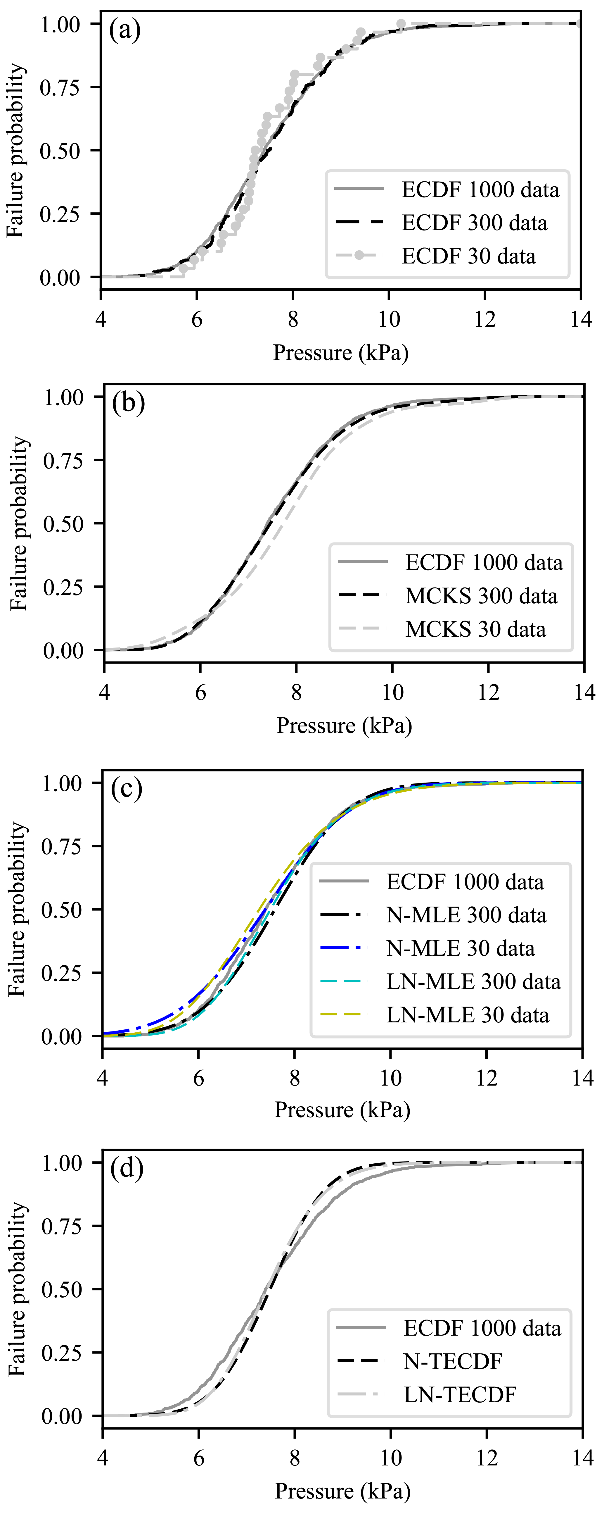
Figure 9 Reliability method comparisons between empirical cumulative distribution functions (ECDF) with set a) sample of size 1000 and (a) empirical cumulative distribution functions with samples of sizes 30 and 300; (b) Gaussian kernel smoothing (MCKS) cumulative distributions functions with samples of sizes 30 and 300; (c) maximum likelihood estimation cumulative distribution function (MLECDF) fitting of normal (N-MLE) and log-normal (LN-MLE) distributions with samples of sizes 30 and 300; (d) Taylor expansion of the first two centered statistical moments estimates to build normal (N-TE) and log-normal (LN-TE) cumulative distributions functions.
The comparison between each method, presented in Sect. 4, is carried out choosing one set of input distributions, namely set (1.α.a) where all COVs are fixed to 0.05. For the reliability methods using MC simulations (i.e., ECDF, MLECDF and MCKS), the number of simulations is set to 30, 300, and 1000, respectively. The ECDF method is the most robust and its accuracy increases with the MC sample size (Fig. 9a). Thus, the reference fragility curve is the one derived from the 1000 simulations ECDF sample.
We defined the fragility range as the interval between the 2.5 % and 97.5 % quantile of the limit pressure CDF, i.e., the pressure range in which the fragility increases from ≈0 to ≈1. Depending on the fragility range width, a relatively high number of simulations may be needed in order to obtain smooth fragility curves. Since the MCKS method, by definition, smooths the CDF curve approximation, fewer simulations are required than with ECDF method in order to obtain such smooth curves (Fig. 9b). The same conclusion can be drawn in the case of MLECDF method, which, by definition, always leads to smooth curves. In Fig. 9c, a significant effect of the assumed output CDF can be seen at low simulation numbers, i.e., for a 30-sample data set. The fragility curves provided by normal and log-normal fitting are far from the fragility curves given by the 1000-sample ECDF method. This effect disappears when 300 simulations are performed (Fig. 9c).
In the case of the TECDF method, the approximation of the first statistical moments and the second centered statistical moments combined with normal or log-normal CDF needs only 15 simulations at the first order of the Taylor expansion. One simulation allows the mean to be estimated at the first order and 14 simulations allow the variance to be estimated at the first order. The second order mean estimate needs 113 simulations. For the TECDF method, the approximation of the fragility curve exhibits slight differences compared to the ECDF fragility curve regardless of the assumed output CDF (Fig. 9d). This method is based on the assumption that a good estimator of the output mean of the model can be calculated from the mean of input variables. Observed differences can be due to the non-linearity of the SDOF model. Nevertheless, if non-linearities of the deterministic model are not too significant, few simulations are needed which allows fragility curves to be derived quickly.
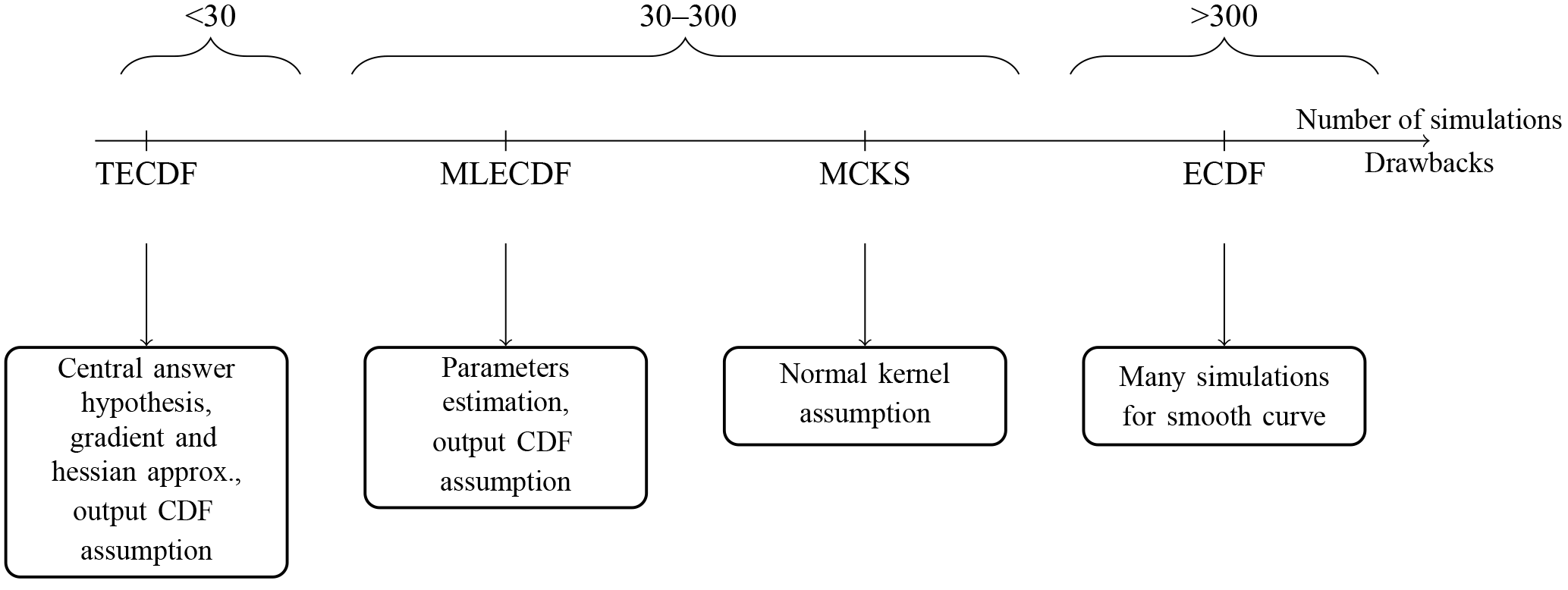
The efficiency and drawbacks of each method are summed up in the scheme of Fig. 10. All in all, the kernel smoothing method appears to be a good compromise. It allows possible non-linearities of the deterministic model to be taken into account and smooth curves to be obtained without too many MC simulations and without any assumption of the shape of the fragility curve. Therefore, it is used for all further sensitivity and parametric studies.
5.2 Fragility curve sensitivity to inputs distributions
5.2.1 Input PDF effect
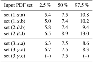
Independent input PDFs give similar fragility curves when they are centered around the same mean input values (Fig. 11a). For the three independent cases, the 50 % quantile is similar and the fragility range varies slightly (Table 4). The greater the COV values, the greater the spread of the fragility curve, a quite intuitive result. Neither the 50 % quantile, nor the fragility range are similar to the latter set (J) for which, for a given pressure, the failure probability is estimated to be significantly lower.

Figure 11 Statistical distributions effects on fragility curves (built with 300 data using the Gaussian Kernel Smoothing method) considering (a) different types of statistical inputs distributions, i.e., sets ( a), ( b), ( b), and ( J) of Table 3, (b) different number of input parameters, i.e., fully deterministic with set ( c), mixed deterministic-statistical with sets (1,α,a) and a), and fully statistical with set a) of Table 3.
Table 4 The 2.5,%, 50 %, and 97.5 % quantiles (in kPa) of the fragility curve according to the input PDF reference set.
5.2.2 Number and class of random variables
Four combinations are considered to investigate the effect of the number and the class of random variables, i.e., (i) the deterministic case, set c), which is taken as the reference fragility curve; (ii) only geometrical inputs are assumed to be deterministic with set a); (iii) only the material strength parameters are described as random variables with set a); and finally, (iv) all the input variables are considered as random variables with set a). Results are presented in Fig. 11b. The number of random input parameters controls the spread of the fragility curve (Table 4). If the geometrical uncertainties are not considered, the fragility range drops from [5.4–10.8] to [6.3–8.6] kPa. Assuming a deterministic reinforcement ratio, the fragility range drops from [6.3–8.6] to [6.7–8.3] kPa. The more random input variables that are considered, the wider the fragility range is. Finally, one can notice the asymmetry of the fragility range even if input distributions are symmetric (e.g., normal distributions), which represents the non-linear nature of the problem.
5.3 Effect of physical parameters
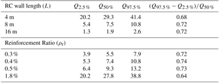
Table 5 The 2.5 %, 50 %, 97.5 % quantiles (in kPa), and the fragility range ratio of the fragility curves according to the length and reinforcement ratio.
5.3.1 Length effect
Figure 12Effects on fragility curves (built with 300 data using the Gaussian Kernel Smoothing method) of the mean values of (a) the length of the RC wall, i.e., 4, 8 and 16 m; and (b) the reinforcement ratio, i.e., 0.3 %, 0.4 %, 0.5 %, and 1.8 %.
The ultimate pressure value (pu) is significantly influenced by the mean length of the RC wall (Fig. 12a). The longer the RC wall, the lower the ultimate pressure (). If the fragility range scope is normalized by the 50 % quantile, such as, for instance , it leads to 0.68, 0.72, and 0.72 for 16, 8, and 4 m, respectively (Table 5).
5.3.2 Reinforcement ratio
The influence of the reinforcement ratio is explored for several typical values. The lower the reinforcement ratio, the lower the ultimate pressure (Fig. 12b). The values of the 50 % quantile are presented in Table 5.
As the reinforcement ratio plays an important role in the failure mode of the structure, a high density reinforcement ratio is tested, such as ρr=1.8 %. For a low reinforcement ratio, e.g., <1 %, the failure of the RC wall occurs when the ultimate strain within steel is reached. On the contrary, for a high reinforcement ratio, the concrete reaches its ultimate strain first. This aspect is implicitly taken into account by the bending moment–curvature relationship. Nevertheless, for highly reinforced RC walls, the failure mode can change depending on the magnitude of traversal shearing forces, i.e., along the y axis, and thus a bending failure mode may be questionable when the length of the RC wall becomes small.
5.3.3 Avalanche loading rate
Depending on the RC wall mechanical properties and on the avalanche loading time evolution, inertial effects can develop and modify the structural response through time. In order to assess the effect of the avalanche loading rate (τ), three values were tested: 3, 6, and 9 kPa s−1. Resulting fragility curves are depicted in Fig. 13 and compared to the quasi-static case investigated so far (lower loading rate). For higher loading rates, inertial effects appear and lead to an increase of the apparent structural strength. The fragility curve is shifted to the right with the increase of the loading rate, which suggests that under dynamic loading conditions the structure is safer (i.e., able to support higher peak pressures). However, it must be kept in mind that the considered time evolution of the pressure is triangular (Fig. 1b). Thus, for high loading rates, the duration of the applied pressure becomes shorter. With longer loading durations, for instance using a trapezoidal pressure signal through time, the fragility curves can be affected in a different way. Thus, the increase of resistance of the structure with the loading rates, which is herein showed, can not be generalized. One of the advantages of the proposed SDOF model is that any kind of pressure time evolutions can be applied onto the structure and thus the effect of the pressure signal on fragility curves can be easily investigated.
Figure 13Effects on fragility curves of the avalanche loading rate. Fragility curves have been computed using the ECDF reliability method.
Very few snow avalanche fragility and vulnerability curves have been reported in the literature. However, to put our results in a broader perspective, the herein obtained fragility curves were plotted against existing curves. First, the numerical fragility curves proposed by Favier et al. (2014) were considered (Fig. 14a). The expert judgmental fragility curves proposed by Wilhelm (1998) and, finally, the vulnerability curves proposed by Keylock et al. (1999) and Barbolini et al. (2004) were subsequently considered (Fig. 14b–c).
Figure 14Comparison of the article fragility curve to (a) the numerical fragility curves from Favier et al. (2014), (b) the expert judgmental fragility curves of Wilhelm (1998), and (c) the vulnerability curves of Barbolini et al. (2004) and Keylock et al. (1999). The exact meaning of each curve is provided in text.
Based on classical engineering approaches, Favier et al. (2014) obtained ultimate pressures related to four typical limit states of an RC structure. The limit state “Elast” is related to the reach of the elastic limit within the RC wall. Limit state “ULS” and “ALS” is based on the classical definition of the ultimate and accidental limit state given in Eurocode 2, respectively, which allows the ultimate pressure to be calculated, considering safety coefficients related to strength parameters of the RC wall. The last limit state allows the collapse pressure deduced from the classical yield line theory (“YLT”) to be obtained. Several boundary conditions were investigated (i.e., clamped edges, simply supported edges, free edges, and a combination of all three). The comparison with our results is presented in Fig. 14a. The same input PDFs have been considered in both studies, where the COVs are equal to 0.05 for all random variables (cf. set a)). The fragility curve obtained in this work shows that the structure collapses for lower pressure values than those found in Favier et al. (2014). This difference is mainly due to the discrepancy of boundary conditions between the RC walls considered within both approaches. Indeed, a one-way slab configuration leads to a lower structural capacity than those considered by Favier et al. (2014), which were mostly two-way RC slabs.
Wilhelm (1998) built fragility curves for reinforced concrete structures according to expert information. This was done by associating three and four pressures with three and four typical damage thresholds, respectively, i.e., a lower damage threshold, a general damage threshold and a specific demolition limit (additionally, a specific destruction limit). The resulting curves are plotted in Fig. 14b, i.e., curves “Concrete with reinforcement – 1” and “Reinforced” and curves “Concrete with reinforcement – 2”, respectively. Compared to these, the herein obtained fragility curves is shifted to the left by approximately 18 to 32 kPa and has a wider dispersion. In addition, the shapes of the curves are different. The curves obtained by Wilhelm (1998) are piecewise linear functions whereas the herein obtained fragility curve is a smooth differentiable function.
Keylock et al. (1999) and Barbolini et al. (2004) proposed empirical fragility curves constructed using a method derived from the seismic engineering field and least squares regression. This allowed linking snow avalanche damage data from Iceland and Austria, respectively, to the specific loss. Compared to these, as for Wilhelm (1998)'s curves, our fragility curve is shifted to the left, less dispersed, and has a smoother shape.
Many points can explain the differences in shapes and values between all these curves. Indeed, even if some similarity is expected, all curves, especially those representing the failure probability on the one hand and the sensitivity of damage as function of avalanche pressure on the other, do not necessarily have to follow the same trends. Specifically, several factors can explain the differences we highlighted.
First, the failure probability gives the probability that the structure exceeds the ultimate damage state, whereas the sensitivity of damage gives a deterministic value of damage ratio, which is rather different. For instance, it can be assumed that the expert in Wilhelm (1998) has chosen, for safety reasons, pressure thresholds from the tail of the pressure distribution, which could explain the shift with regards to our results. Second, numerical fragility or vulnerability curves result from the uncertainty and variability assumptions made by those performing the measurements (e.g., for materials, geometries), whereas empirical curves sum-up the uncertainty and variability resulting from the available field data (e.g., variability of damages among one given damage state category of a building, epistemic uncertainties, variabilities among damaged buildings in the avalanche signal for a given avalanche, or from one avalanche to another), and these do not necessarily correspond. Third, even if all the considered (real or numerical) buildings fall in the “reinforced concrete” typology, their technologies of construction may have been quite different. For instance, little information is provided by Wilhelm (1998), which may imply that the materials and the geometries considered were in fact rather different than others such as Barbolini et al. (2004).
This paper presents the derivation of fragility curves for a reinforced concrete wall loaded by a dynamic pressure field due to a snow avalanche. Methods from the reliability framework have been implemented and combined with a simplified SDOF model, which is light and efficient. A one-way simply supported RC wall has been considered and a deterministic model based on an equivalent mass-spring system has been used to represent its mechanical behavior up to the rupture when subjected to a uniform pressure field. The ability of the SDOF model to predict the RC wall mechanical response has been validated based on comparisons with FEA and limit analyses. Using a SDOF approach significantly reduces the computation time needed to perform a single simulation and allows accounting for the physics involved up to the collapse of the structure during wall–avalanche interactions. Second, four reliability methods have been implemented to derive fragility curves. All methods gave similar results regardless of the configuration considered, at least for the core of the distribution. The advantages and drawbacks of each method have been identified, and the kernel smoothing method was selected as a reasonable compromise for further parametric and sensitivity studies. This comprehensive framework could be valuable for a wide range of reliability-based engineering applications where structural members are loaded by non-uniform pressure fields which can evolve through time.
For our specific snow avalanche case study, systematic fragility curves were derived. The results emphasize that fragility curves are very sensitive to physical parameters such as the RC wall's geometry, its reinforcement ratio or the loading features. In particular, the spread of the fragility range appeared to be strongly variable. However, as soon as the fragility range was standardized by its 50 % quantile, the relative fragility spread remained almost the same. These results supplement the few fragility and vulnerability curves already available in snow avalanche engineering literature. They will be of great value for future works that seek to refine formal risk evaluation in avalanche prone areas.
According to the scarce available measurement data, it was assumed that the response of the structure was quasi-static. The SDOF model formulation has been made within a dynamic framework. The proposed SDOF model is thus able to describe the occurrence of potential additional resisting forces (structural inertia), which are governed by the pressure time evolution. The effect of the latter was explored, underlining the increase of the apparent strength with the loading rate when triangular pressure time evolutions are considered and high loading rates are imposed onto the RC wall. As this result cannot be generalized, further research is needed to explore the influence of various pressure time evolutions on the fragility curves derivation. Moreover, our approach can be implemented for other types of structures with different technologies (e.g., other RC structure configurations, masonry, timber or metallic structures) and/or more sophisticated structure geometries. Finally, extension to other mass movements hazards such as debris flows, rockfalls or ice avalanches, for which similar gaps in engineering need to be filled, may be pursued. It should be kept in mind that for each hazard, the challenge will be to propose simplified mechanical models able to account for the main physics with a reduced computation time.
As a perspective, the main difficulty concerns the modeling of the avalanche pressure, which can vary significantly as function of meteorological conditions and especially in terms of pressure magnitude, spatial distribution and typical time of variation. Pressure magnitude is implicitly taken into account by the fragility curves but the spatial distribution and pressure variations through time can have a significant influence on the structure mechanics. The structure's mechanical features are generally better known than the avalanche loading. Thus, further research, accounting for several typical spatial distributions and time evolutions of the pressure, might be of specific interests to highlight the influence of avalanche loadings on curves, which are used in formal risk evaluation.
Data of the curves from Figs. 11 and 12 can be freely accessed on the website http://www.avalanches.fr/mopera-production-et-delivrables/ (French Ministry in charge of the environment, 2018).
DB and NE designed the research. DB and PF planned and carried out the simulations. All authors contributed to the analysis of the results and to the writing of the manuscript.
The authors declare that they have no conflict of interest.
The authors are grateful to the ANR research program MOPERA (MOdélisation Probabiliste pour l'Etude du Risque d'Avalanche),
the MAP3 ALCOTRA INTERREG program, the Chilean National Commission for Scientific and Technological Research (CONICYT) under
grant Redes 150119 and grant Fondecyt Postdoc 3160483, the Chilean National Research Center for Integrated Natural Disaster
Management CONICYT/FONDAP/15110017 (CIGIDEN), and the ECOS-CONICYT Scientific cooperation program under project “Multi-risk
assessment in Chile and France: application to seismic engineering and mountain hazards ECOS170044 and ECOS action
C17U02”
for financially supporting this work. Irstea is member of Labex Osug@2020.
Edited by: Perry Bartelt
Reviewed by: four anonymous referees
Au, S.-K. and Beck, J. L.: Estimation of small failure probabilities in high dimensions by subset simulation, Probabilist. Eng. Mech., 16, 263–277, 2001. a
Barbolini, M., Cappabianca, F., and Sailer, R.: Empirical estimate of vulnerability relations for use in snow avalanche risk assessment, in: Risk Analysis IV, edited by: Brebbia, CA, vol. 9 of Management Information Systems, 4th International Conference on Computer Simulation in Risk Analysis and Hazard Mitigation, Rhodes, Greece, 27–29 September 2004, 533–542, 2004. a, b, c, d, e
Bartelt, P., Bebi, P., Feistl, T., Buser, O., and Caviezel, A.: Dynamic magnification factors for tree blow-down by powder snow avalanche air blasts, Nat. Hazards Earth Syst. Sci., 18, 759–764, https://doi.org/10.5194/nhess-18-759-2018, 2018. a
Baudin, M., Dutfoy, A., Iooss, B., and Popelin, A.-L.: OpenTURNS: An industrial software for uncertainty quantification in simulation, Handbook of Uncertainty Quantification, 2001–2038, 2017. a
Bellot, H., Bouvet, F. N., Naaim, M., Caccamo, P., Faug, T., and Ousset, F.: Taconnaz avalanche path: pressure and velocity measurements on breaking mounds, in: International Snow Science Workshop (ISSW), Irstea, ANENA, Meteo France, 1378–1383, 2013. a
Berthet-Rambaud, P.: Structures rigides soumises aux avalanches et chutes de blocs: modélisation du comportement mécanique et caractérisation de l'interaction phénomène-ouvrage, PhD thesis, Université Grenoble 1 – Joseph Fourier, 2004. a
Berthet-Rambaud, P., Limam, A., Baroudi, D., Thibert, E., and Taillandier, J.-M.: Characterization of avalanche loading on impacted structures: a new approach based on inverse analysis, J. Glaciol., 54, 324–332, 2008. a, b
Bertrand, D., Naaim, M., and Brun, M.: Physical vulnerability of reinforced concrete buildings impacted by snow avalanches, Nat. Hazards Earth Syst. Sci., 10, 1531–1545, https://doi.org/10.5194/nhess-10-1531-2010, 2010. a, b
Biggs, J.: Introduction to structural dynamics, New York: McGraw-Hill Book Company, 1964. a, b, c, d
Cappabianca, F., Barbolini, M., and Natale, L.: Snow avalanche risk assessment and mapping: A new method based on a combination of statistical analysis, avalanche dynamics simulation and empirically-based vulnerability relations integrated in a GIS platform, Cold Reg. Sci. Technol., 54, 193–205, https://doi.org/10.1016/j.coldregions.2008.06.005, 2008. a
Carta, G. and Stochino, F.: Theoretical models to predict the flexural failure of reinforced concrete beams under blast loads, Eng. Struct., 49, 306–315, 2013. a
Eckert, N., Parent, E., Faug, T., and Naaim, M.: Optimal design under uncertainty of a passive defense structure against snow avalanches: from a general Bayesian framework to a simple analytical model, Nat. Hazards Earth Syst. Sci., 8, 1067–1081, https://doi.org/10.5194/nhess-8-1067-2008, 2008. a
Eckert, N., Parent, E., Faug, T., and Naaim, M.: Bayesian optimal design of an avalanche dam using a multivariate numerical avalanche model, Stoch. Environ. Res. Risk A., 23, 1123–1141, 2009. a
Eckert, N., Keylock, C. J., Bertrand, D., Parent, E., Faug, T., Favier, P., and Naaim, M.: Quantitative risk and optimal design approaches in the snow avalanche field: Review and extensions, Cold Reg. Sci. Technol., 79, 1–19, 2012. a
Ellingwood, B. R.: Earthquake risk assessment of building structures, Reliability Engineering and System Safety, 74, 251–262, 2001. a
Favier, P., Bertrand, D., Eckert, N., and Naaim, M.: A reliability assessment of physical vulnerability of reinforced concrete walls loaded by snow avalanches, Nat. Hazards Earth Syst. Sci., 14, 689–704, https://doi.org/10.5194/nhess-14-689-2014, 2014. a, b, c, d, e, f, g
Favier, P., Eckert, N., Faug, T., Bertrand, D., and Naaim, M.: Avalanche risk evaluation and protective dam optimal design using extreme value statistics, J. Glaciol., 62, 725–749, https://doi.org/10.1017/jog.2016.64, 2016. a
Favre, R., Jaccoud, J., Burdet, O., and Charif, H.: Dimensionnement des structure en béton – Aptitude au service et éléments de structures, Presses Polytech. et Univ. Romandes, 1990. a, b
French Ministry in charge of the environment, avalanches.fr, available at: http://www.avalanches.fr/mopera-production-et-delivrables/, last access: 7 September 2018.
Fisher, R. A.: On the Mathematical Foundations of Theoretical Statistics, Philos. T. Roy. Soc. Lond. A, 222, 309–368, 1922. a
Johansen, K.: Yield Line Theory, Cement and Concrete Association, London, UK, 1962. a
Joint Committee on Structural Safety, JCSS: Probabilistic Model Code, Part I–III, available at: http://www.jcss.byg.dtu.dk/Publications/Probabilistic_Model_Code, last access: 7 August 2018, 2001. a
Jones, J., Wu, C., Oehlers, D., A.S. Whittaker, A. W. S., Marks, S., and Coppola, R.: Finite difference analysis of simply supported RC slabs for blast loadings, Eng. Struct., 31, 2825–2832, 2009. a
Kassem, F., Bertrand, D., Brun, M., and Limam, A.: Reliability analysis of reinforced concrete slab subjected to low velocity impact accounting of material damage, 11th International Conference on Structural Safety & Reliability – Columbia University – New York, NY, 2013. a
Keylock, C. and Barbolini, M.: Snow avalanche impact pressure – Vulnerability relations for use in risk assessment, Can. Geotech. J., 38, 227–238, 2001. a
Keylock, C. J., McClung, D. M., and Magnússon, M. M.: Avalanche risk mapping by simulation, J. Glaciol., 45, 303–314, https://doi.org/10.1017/S0022143000001805, 1999. a, b, c, d
Kyung, H. L. and Rosowsky, D. V.: Fragility analysis of woodframe buildings considering combined snow and earthquake loading, Struct. Saf., 28, 289–303, 2006. a
Lagaros, N. D.: Probabilistic fragility analysis: A tool for assessing design rules of RC buildings, Earthq. Eng. Eng. Vib., 7, 45–56, 2008. a
Lemaire, M.: Fiabilité des structures – Couplage mécano-fiabiliste statique, 2005. a, b
Li, Y. and Ellingwood, B. R.: Reliability of woodframe residential construction subjected to earthquakes, Struct. Saf., 29, 294–307, https://doi.org/10.1016/j.strusafe.2006.07.012, 2007. a
Low, H. Y. and Hao, H.: Reliability analysis of reinforced concrete slabs under explosive loading, Struct. Saf., 23, 157–178, 2001. a
Low, H. Y. and Hao, H.: Reliability analysis of direct shear and flexural failure modes of RC slabs under explosive loading, Eng. Struc., 24, 189–198, 2002. a, b
Lu, R., Luo, Y., and Conte, J.: Reliability evaluation of reinforced concrete beams, Struct. Saf., 14, 277–298, 1994. a
MacGregor, J. G., Mirza, S. A., and Ellingwood, B.: Statistical analysis of resistance of reinforced and prestressed concrete members, ACI Journal, 80, 167–176, 1983. a
Mattock, A. H.: Discussion of rotational capacity of reinforced concrete beams, Journal of Structual Division, 93, 519–522, 1967. a
Mavrouli, O. and Corominas, J.: Rockfall vulnerability assessment for reinforced concrete buildings, Nat. Hazards Earth Syst. Sci., 10, 2055–2066, https://doi.org/10.5194/nhess-10-2055-2010, 2010a. a
Mavrouli, O. and Corominas, J.: Vulnerability of simple reinforced concrete buildings to damage by rockfalls, Landslides, 7, 169–180, 2010b. a
Melchers, R.: Importance sampling in structural systems, Struct. Saf., 6, 3–10, 1989. a
Millard, A.: CASTEM 2000, Manuel d'utilisation, Rapport no CEA-LAMBS 93/007, Commissariat à l'Energie Atomique, Saclay, available at: http://www-cast3m.cea.fr (last access: 29 August 2018), 1993. a
Mirza, S., Hatzinikolas, M., and MacGregor, J.: Statistical descriptions of strength of concrete, J. Struct. Div.-ASCE, 105, 1021–1037, 1979. a
Newmark, N.: A Method of Computation for Structural Dynamics, J. Eng. Mech.-ASCE, 85, 67–94, 1959. a
Ngo, T., Mendis, P., Gupta, A., and Ramsay, J.: Blast loading and blast effects on structures – An overview, J. Struct. Eng., 7, 76–91, 2007. a
Ousset, I., Bertrand, D., Brun, M., Limam, A., and Naaïm, M.: Vulnerability of a reinforced concrete wall loaded by a snow avalanche: experimental testing and FEM analysis, International Snow Science Workshop Grenoble – Chamonix Mont-Blanc – 2013, 2013. a
Ousset, I., Bertrand, D., Eckert, N., Bourrier, F., Naaim, M., and Limam, A.: Vulnérabilité d'une structure de protection contre les avalanches de neige en béton armé – Influence des effets inertiels sur les courbes de fragilité, JFMS 2016 – Nancy, 2016 (in French). a, b
Papathoma-Köhle, M., Kappes, M., Keiler, M., and Glade, T.: Physical vulnerability assessment for alpine hazards: state of the art and future needs, Nat. Hazards, 58, 645–680, https://doi.org/10.1007/s11069-010-9632-4, 2011. a
Papathoma-Köhle, M., Keiler, M., Totshing, R., and Glade, T.: Improvement of vulnerability curves using data from extreme events: debris flow event in South Tyrol, Nat. Hazards, 64, 2083–2105, 2012. a
Rossetto, T. and Elnashai, A.: Derivation of vulnerability functions for European-type RC structures based on observational data, Eng. Struct., 25, 1241–1263, https://doi.org/10.1016/S0141-0296(03)00060-9, 2003. a
Schaerer, P. A. and Salway, A. A.: Seismic and impact–pressure monitoring of flowing avalanches, J. Glaciol., 26, 179–187, 1980. a
Sovilla, B., Schaer, M., Kern, M., and Bartelt, P.: Impact pressures and flow regimes in dense snow avalanches observed at the Vallée de la Sionne test site, J. Geophys. Res., 113, F01010, https://doi.org/10.1029/2006JF000688, 2008. a, b
Sovilla, B., McElwaine, J., Steinkogler, W., Hiller, M., Dufour, F., Surinach, E., Perez-Guillen, C., Fischer, J., Thibert, E., and Baroudi, D.: The full-scale avalanche dynamics test site Vallée de la Sionne, in: International Snow Science Workshop Grenoble – Chamonix Mont-Blanc, 2013. a
Sudret, B. and Mai, C.: Computing seismic fragility curves using polynomial chaos expansions, in: 11th International Conference on Structural Safety and Reliability (ICOSSAR 2013), 3337–3344, 2013. a
Thibert, E. and Baroudi, D.: Impact energy of an avalanche on a structure, Ann. Glaciol., 51, 45–54, 2010. a
Thibert, E., Bellot, H., Ravanat, X., Ousset, F., Pulfer, G., Naaim, M., Hagenmuller, P., Naaim-Bouvet, F., Faug, T., Nishimura, K., Baroudi, D., Prokop, A., Schon, P., Soruco, A., Vincent, C., Limam, A., and Heno, R.: The full-scale avalanche test-site at Lautaret Pass (French Alps), Cold Reg. Sci. Technol., 115, 30–41, 2015. a
Val, D., Bljuger, F., and Yankelevsky, D.: Reliability evaluation in nonlinear analysis of reinforced concrete structures, Struct. Saf., 19, 203–217, 1997. a, b, c
Wand, M. and Jones, M.: Kernel smoothing, ISBN: 0-412-55270-1, edited by: Wand, M. P. and Jones, M. C., Chapman&Hall, London, 1995. a
Wilhelm, C.: Quantitative risk analysis for evaluation of avalanche protection projects, in: 25 Years of Snow Avalanche Research at NGI, proceedings anniversary conference, Voss, 12–16 May 1998, edited by: Hestness, E., 25, 288–293, 1998. a, b, c, d, e, f, g, h