Seismic assessment of a multi-span steel railway bridge in Turkey based on nonlinear time history

Many research studies have shown that bridges are vulnerable to earthquakes, graphically confirmed by incidents such as the San Fernando (1971 USA), Northridge (1994 USA), Great Hanshin (1995 Japan), and Chi-Chi (1999 Taiwan) earthquakes, amongst many others. The studies show that fragility curves are useful tools for bridge seismic risk assessments, which can be generated empirically or analytically. Empirical fragility curves can be generated where damage reports from past earthquakes are available, but otherwise, analytical fragility curves can be generated from structural seismic response analysis. Earthquake damage data in Turkey are very limited, hence this study employed an analytical method to generate fragility curves for the Alasehir bridge. The Alasehir bridge is part of the Manisa–Uşak–Dumlupınar–Afyon railway line, which is very important for human and freight transportation, and since most of the country is seismically active, it is essential to assess the bridge's vulnerability. The bridge consists of six 30 m truss spans with a total span 189 m supported by 2 abutments and 5 truss piers, 12.5, 19, 26, 33, and 40 m. Sap2000 software was used to model the Alasehir bridge, which was refined using field measurements, and the effect of 60 selected real earthquake data analyzed using the refined model, considering material and geometry nonlinearity. Thus, the seismic behavior of Alasehir railway bridge was determined and truss pier reaction and displacements were used to determine its seismic performance. Different intensity measures were compared for efficiency, practicality, and sufficiency and their component and system fragility curves derived.

1 Introduction

Fragility is the conditional probability that a structure or structural component will meet or exceed a certain damage level for a given ground motion intensity, such as peak ground acceleration (PGA) or spectral acceleration (S_a). Thus, fragility analysis is an important tool to determine bridge seismic vulnerability (Pan et al., 2007). Fragility curves can be derived by three methods: expert base, empirical, and analytical. Analytical fragility curves are usually expressed in the form of two-parameter lognormal distributions (Shinozuka et al., 2000b), whereas empirical and expert base curves are generally based on the damage state given the observed ground motion intensity as determined by an expert (Shinozuka et al., 2000b). When the damage state and ground motion intensity is unknown, analytical methods are used to determine these, and analytical fragility curves subsequently derived (Nielson, 2005).

An important issue when deriving fragility curves is determining the relation between the intensity measure (IM) and engineering demand parameter (EDP), which can be different depending on the specific case. Three methods are commonly employed to determine this: nonlinear time history, incremental dynamic, and capacity spectrum analyses, with time history analysis being the most commonly used tool (Banerjee and Shinozuka, 2007; Bignell et al., 2004; Shinozuka et al., 2000a; Mackie and Stojadinović, 2001; Kumar and Gardoni, 2014). Incremental dynamic analysis can also be used to determine the earthquake response of a structure and derive the fragility curve (Lu et al., 2004; Kurian et al., 2006; Liolios et al., 2011). Time history analysis gives more realistic results, but both time history and incremental dynamic analysis are time-consuming and computationally expensive. Therefore, capacity spectrum analysis is sometimes used to quickly derive the fragility curve (Banerjee and Shinozuka, 2007; Shinozuka et al., 2000a).

Determining fragility curves for retrofitted bridge systems, along with component and system fragility are other issues currently attracting research attention (Padgett et al., 2007a; Chuang-Sheng et al., 2009; Alam et al., 2012; Tsubaki et al., 2016), and the energy-based approach has also been employed recently for fragility analysis (Wong, 2009). In addition, analytical methods and decision mechanisms are established to determine the most appropriate method for reducing earthquake risk (Dan, 2016).

Damage state of bridges after earthquake exposure can be estimated using expert and analytical based methods. Expert-based methods depend on past earthquake and damage data recorded in seismic events (Shinozuka et al., 2000c), whereas analytical methods depend on the nonlinear analysis. Earthquake data incorporate displacement and rotation, and damage state displacement and rotation limits must be determined (Choi and Jeon, 2003; Padgett et al., 2007b; Pan et al., 2007).

This paper describes nonlinear behavior and derives the fragility curves for a selected railway bridge. The bridge is critical for railway transportation and its unique structural designation, being constructed almost 100 years ago, increases its importance. We followed Cornell et al. (2002) to derive the bridge fragility curve, considering different IMs and determined the most suitable IM. Capacity and serviceability limits were then used to derive the fragility curve. Component and system fragility curves were derived separately.

2 Analytical method and simulation

Fragility curves are effective tools to determine seismic capacity of structures or structural components. Fragility is defined as the conditional probability of seismic demand (the specific EDP in this case) on the structure or structural component exceeding its capacity, C, for a given level of ground motion intensity (Padgett and DesRoches, 2008),

$$\begin{array}{}\text{(1)}& {\displaystyle }{\displaystyle }\mathrm{Fragility}=P[\mathrm{EDP}\ge C\left|\mathrm{IM}\right.],\end{array}$$

where P(…) is the probability of the particular case. Probability seismic demand models (PSDMs) were determined using nonlinear time history analysis to model and analyze the bridge structure and determine the bridge structural demand and capacity.

2.1 Probabilistic seismic demand model

A PSDM describes the seismic demand of a structure or structural component in terms of an approximate IM (Padgett and DesRoches, 2008),

$$\begin{array}{}\text{(2)}& {\displaystyle }{\displaystyle }P[\mathrm{EDP}\ge d\left|\mathrm{IM}\right.]=\mathrm{1}-\mathit{\varphi }\left({\displaystyle \frac{\ln \left(d\right)-\ln \left(\widehat{\mathrm{EDP}}\right)}{{\mathit{\beta }}_{\mathrm{EDP}\left|\mathrm{IM}\right.}}}\right),\end{array}$$

where the median EDP was estimated as a power model,

$$\begin{array}{}\text{(3)}& {\displaystyle }{\displaystyle }\widehat{\mathrm{EDP}}=a{\mathrm{IM}}^b,\end{array}$$

or linear logarithm model,

$$\begin{array}{}\text{(4)}& {\displaystyle }{\displaystyle }\ln \left(\mathrm{EDP}\right)=\ln \left(a\right)+b\ln \left(\mathrm{IM}\right),\end{array}$$

where a and b are regression coefficients, ϕ is the standard normal cumulative distribution function, $\widehat{\mathrm{EDP}}$ is the median value of engineering demand, d is the limit state to determine the damage level and β_EDP|IM (dispersion) is the conditional standard deviation of the regression (Siqueira et al., 2014),

$$\begin{array}{}\text{(5)}& {\displaystyle }{\displaystyle }{\mathit{\beta }}_{\mathrm{EDP}\left|\mathrm{IM}\right.}\cong \sqrt{{\displaystyle \frac{\sum {\left(\ln \left(d_i\right)-\ln \left(a{\mathrm{IM}}^b\right)\right)}^{\mathrm{2}}}{N-\mathrm{2}}}}.\end{array}$$

2.2 Component and system fragility

Component fragility describes the seismic behavior of different components under the same level of damage and allows the weakest bridge component to be determined. Buckling capacities of all members were calculated, and fragility curves for Truss Piers, Trusses, and Stringer members were derived using PSDMs. Truss piers are the most fragile component because of their total length and the slenderness of their elements.

However, the point of system fragility is to determine all possible damage probabilities in the system, since all components must be considered to derive the overall bridge fragility curve. Bridge damage probability for a chosen limit state is the union of probabilities of each component for the same limit state (Nielson and DesRoches, 2007),

$$\begin{array}{}\text{(6)}& {\displaystyle }{\displaystyle }P\left[{\mathrm{Fail}}_{\mathrm{system}}\right]=\bigcup _{i=\mathrm{1}}^{n}P\left[{\mathrm{Fail}}_{\mathrm{component}-i}\right].\end{array}$$

Correlation coefficients between EDPs and IMs were considered to follow the conditional joint normal distribution, and system fragility curves were derived using Eq. (6) on 10⁶ demand samples generated by Monte Carlo simulation.

Figure 1 Bridge project plan from 1923.

Figure 2 Current photos of the bridge from Fig. 1.

3 Case study

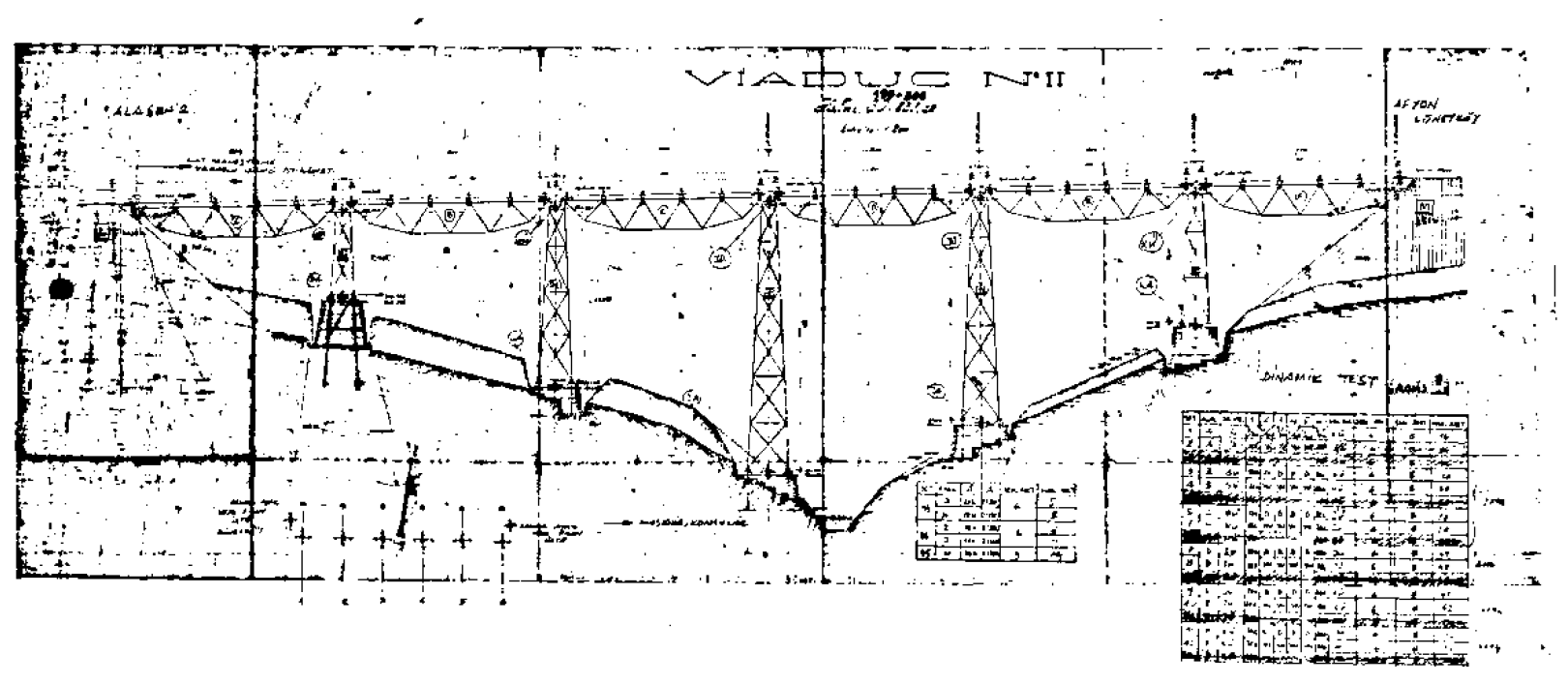
Railway construction in Turkey started with the contribution of European countries such as England, France, and Germany, with the first aim to transport agricultural goods and valuable minerals to Europe from the harbors. The first railroad line was constructed by an English company in 1856 on the İzmir–Aydın corridor with total length 130 km (Fig. 1 shows project plans of the case bridge and Fig. 2 shows current photos of the bridge. The railroad system in Turkey is divided into 7 regions, with total length 8722 km, and 81 % of the 25 443 culverts and bridges were built before 1960, some certified as having historical significance.

The Alasehir bridge is part of the Manisa–Uşak-Dumlupınar–Afyon railroad line, which is approximately 200 km long, and was built by the Ateliers De Construction De Jambes Namur Company in 1923. The bridge is composed of 6 steel truss sub-bridges with 30 m span each and has 5 truss piers 12.5, 19, 26, 33, and 40 m high. The total length of the bridges is 189 m and has 300 m horizontal curve radius. The road curvature is applied via the rail location on the trusses, and this is why one side truss strength is higher than the other side truss. The railroad slope is approximately 2.7 %. The truss systems are simply supported between abutment to pier, pier to pier, and pier to abutment. The piers are connected to the foundation with long and thick steel anchorages. The bridge was constructed using angle and built-up sections. Spans were constructed from of 80 × 80 × 12, 100 × 100 × 12, 120 × 120 × 11, and 120 × 120 × 15 mm angle; and 20 × 420, 20 × 200, and 20 × 400 mm plate elements. Piers were constructed from 80 × 80 × 10, 100 × 100 × 10, 100 × 100 × 12, 120 × 120 × 12, and 120 × 120 × 14 mm angle; and 300 mm UPN elements. There are walkways at both sides of the sub-spans, and the sleepers rest over stringers mounted onto the transverse girders.

4 Analytical modelling and simulation

4.1 Ground motion suites

The effect of ground motion on the structure was obtained using a linear or nonlinear mathematical model. Nonlinear dynamic time history analysis was used to minimize structural response uncertainties and provide the relationship between ground motion IMs and EDP. These relations can be obtained using cloud (direct) (Shome, 1999), incremental dynamic analysis (IDA) (Vamvatsikos and Allin Cornell, 2002), or stripes (Mackie and Stojadinovic, 2005) methods. This study employed the cloud method, including many real ground motion records, without prior scaling (Mackie et al., 2008).

Figure 3 Earthquake data distribution.

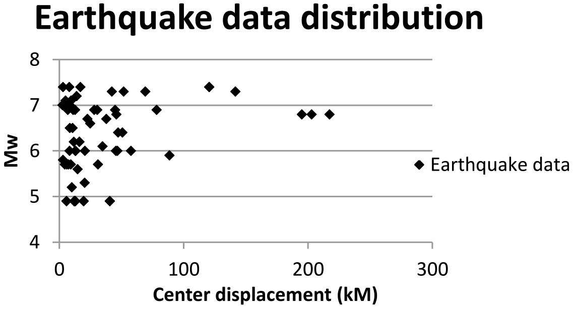
Earthquake data were selected considering different soil types, moment (4.9–7.4), PGAs (0.01–0.82 g), and central distances (2.5–217.4 km). Figure 3 shows the distribution of moment with central distance. Sixty real earthquake data were chosen for soil types A, B, and C, and unscaled earthquake data were used for time history analysis (Pitilakis et al., 2004).

4.2 Analytical bridge models

The bridge elements were modeled by a 2 node beam element. Member support and release were applied according to as-built drawings and site visual inspections. The difference between member center points and connections were all considered as rigid bars account for moments that can occur due to eccentricity.

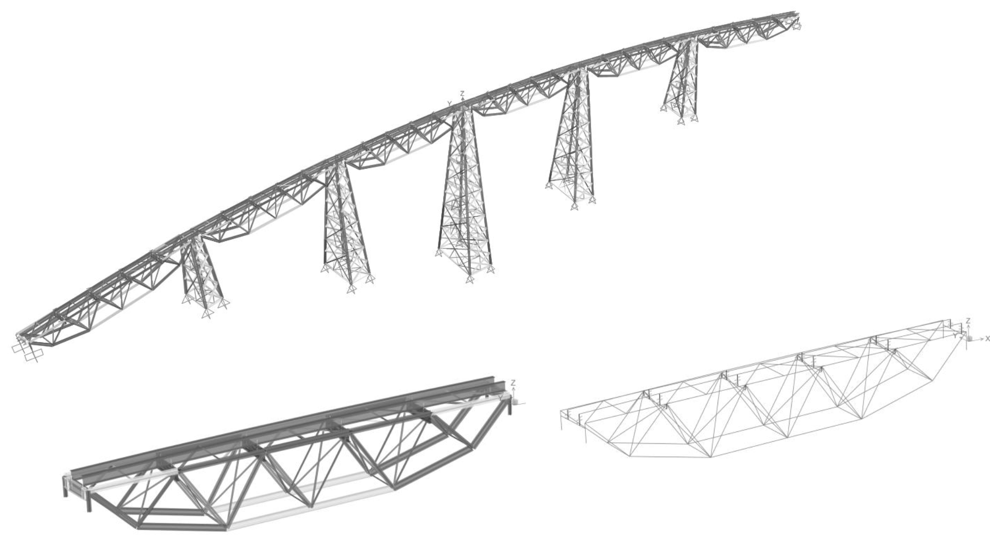
Sleeper and rail profile weights were calculated and applied to the stringer beams as dead load (mass and load). The bridge material was assumed to be ST37 steel, given the construction time. Dead load calculation was performed using the Sap 2000 finite elements software, incorporating the given member properties (area, length, and density). The finite element models were composed of 1609 frame members, 832 nodes, and 120 link elements. A three-dimensional model of the bridge is shown in Fig. 4.

Figure 4 Three-dimensional model of the bridge from Fig. 1.

Time history analyses were applied to the model, considering both material and geometrical nonlinearity. Hinges were defined as steel interacting PMM plastic hinges, as defined in FEMA 356, Eq. (5-4) (FEMA-356, 2000) To detect bridge hazards, plastic hinges were defined at the start, middle, and end points of all frame members. Geometric nonlinearity is defined as Δ − δ, and large displacement Newmark direct integration was employed for the analysis. All three earthquake components (one longitudinal and two horizontal) were defined in the time history process.

5 Selection of intensity measures and demand models

5.1 Selection of intensity measures

PSDMs are traditionally conditioned on a single IM, and the degree of uncertainty depends on the selected IM. Therefore, determining the optimum IM is an important step to derive more realistic fragility curves. There are many different IMs used to characterize seismic behavior, and 9 of the most common, as shown in Table 1, were selected and compared in terms of practicality, efficiency, and proficiency.

Table 1 Intensity measures (IMs).

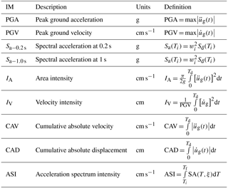
The PGA, PGV, S_a−0.2 s, and S_a−1.0 s IMs are characteristic parameters obtained from earthquake records and related to vector characteristics of ground motion, such as acceleration and velocity. I_A, I_V, CAV, CAD, and ASI IMs are intensity measures characterizing seismic ground motion and are related to ground motion energy (Hsieh and Lee, 2011; Kayen and Mitchell, 1997; Mackie and Stojadinovic, 2004; Özgür, 2009).

Practicality is defined as the correlation between an IM and demand on a structure or structural component, and the more practical intensity measures tend to produce higher correlations. The practicality can be evaluated with the PDSM regression parameter, b, where larger b implies a more practical IM.

Efficiency is defined as the demand alteration for a given IM and can be measured by dispersion, with smaller dispersion implying a higher efficiency IM. Proficiency includes practicality and efficiency (Padgett et al., 2008), defined as modified dispersion,

$$\begin{array}{}\text{(7)}& {\displaystyle }{\displaystyle }\mathit{\zeta }={\displaystyle \frac{{\mathit{\beta }}_{\mathrm{EDP}\left|\mathrm{IM}\right.}}{b}},\end{array}$$

where smaller ζ implies a more proficient IM. Table 2 shows the demand models and intensity.

Table 2 Demand models and intensity measure comparisons.

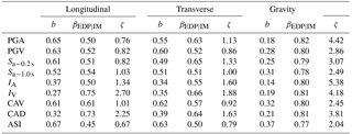
Maximum b = 0.67, 0.63, and 0.37 for the longitudinal, transverse, and gravity directions, respectively. Since higher correlation PSDM provide more realistic results, higher correlation IMs are more practical. Thus, ASI is more practical than other IM options.

Minimum β_EDP|IM = 0.45, 0.50, and 0.77 for the longitudinal, transverse, and gravity directions, respectively. Since smaller dispersion PSDM give more accurate results, smaller dispersion IMs give efficient results. Thus, ASI is more efficient than other IM options. Neilson derive fragility curve for Multi span simply supported (MSSS) steel girder bridge for two suite of ground motions and determine β_EDP|IM as 0.51 and 0.44 for column curvature, which is related to top displacement of bridge. β_EDP|IM obtained in these study gives similar results (Nielson, 2005).

Minimum ζ = 0.67, 0.79, and 2.04 for the longitudinal, transverse, and gravity directions, respectively. Modified dispersion describes IM practicality and efficiency, where smaller ζ implies higher correlation and less dispersion between IMs and EDPs. Thus, ASI is more proficient than other options.

5.2 Probabilistic seismic demand models

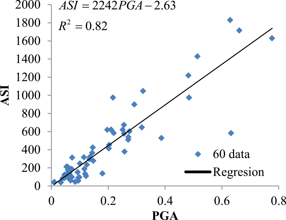
PSDMs were constructed from the peak transverse displacement on the top of the middle pier of the bridge. Sixty nonlinear time history analyses were employed for the selected IM, ASI, following Sect. 5.1. Figures 5 and 6 show there is a good correlation between ASI and transverse displacement of the bridge-middle pier, and ASI and PGA have good correlation, respectively.

Figure 5 PSDMs for selected IMs.

Figure 6 Correlation between ASI and PGA.

5.3 Limit state estimate

There is limited information about damaged steel truss bridges in the literature, but it shows that the main damage causes are buckling of the upper and lower brace elements, and shear failure of the transverse element; with corrosion hastening quickens the phenomena (Kawashima, 2012; Bruneau et al., 1996). Stewart et al. (2009) generated a reliability assessment of a steel truss bridge considering steel element tension and compression capacity as the limit state, calculating the tension capacity as the effective net area of steel members. However, the calculated buckling capacity was found to be smaller than the tension capacity of the members, so the buckling limit is overcome for the compression members during the calculations.

Since there were no specimens tested for the Alasehir bridge, material properties were chosen from previous studies in the literature. Yield and ultimate strength of European railway and roadway bridges are f_y = 200 MPA and F_u = 360 MPa, respectively (Larsson and Lagerqvist, 2009). Structural element capacities for the Alasehir bridge were subsequently calculated depending on geometrical and material properties.

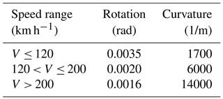
Seismic action may cause train derailment or even overturn, e.g. 1999 Kocaeli Turkey earthquake (Byers, 2004). Therefore, this study also considered serviceability, considering lateral displacement as the serviceability limit state. EN1990-Annex A2 includes lateral displacement limits for railway bridges (EN1990-prANNEX A2, 2001), including maximum angular variation and minimum radius of curvature to limit lateral displacement for different velocities, as shown in Table 3.

Table 3 Maximum angular variation and minimum radius of curvature.

6 Fragility curve for railway serviceability and bridge components

6.1 Fragility curve for railway serviceability

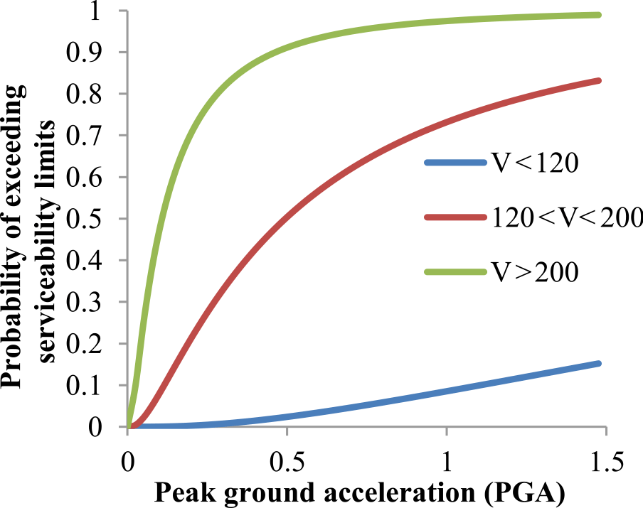
Derailment and overturning can occur under seismic conditions, with 3 such events observed for the Kocaeli, Turkey earthquake (Byers, 2004). Proscribed serviceability limits to minimize such events were used as the limit state in this study (EN1990-prANNEX A2, 2001), considering speed ranges (km h⁻¹) V < 120, 120 < V < 200, and 200 < V. Railway transport has become more important for both goods and humans, and service speed affects transport capacity and quality (Lindfeldt, 2015)

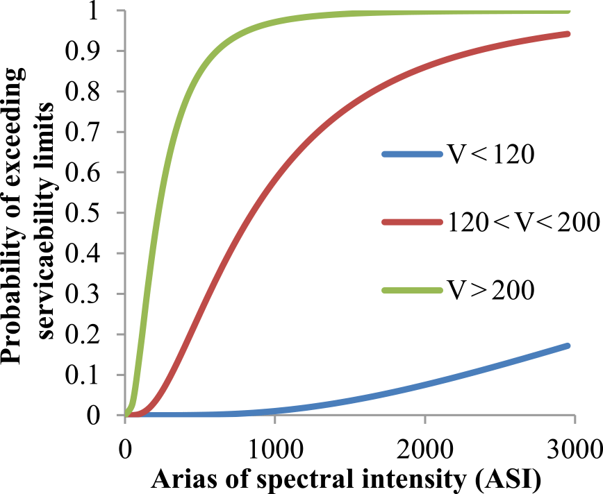
Figures 7 and 8 show the probability of exceeding of serviceability limit states. The 50 % probability of exceeding the serviceability limits occurs for V > 200 km h⁻¹ at ASI = 250 cm s⁻¹ (Fig. 7) and PGA = 0.11 g (Fig. 8) for V > 200 km h⁻¹, ASI = 850 cm s⁻¹ and PGA = 0.5 g for PGA for 120 < V < 200 km h⁻¹, and ASI = 6250 cm s⁻¹ and PGA = 4.8 g for V < 120 km h⁻¹. There is good correlation between ASI and PGA (Sect. 5.2). Median values for V > 200 km h⁻¹ at PGA = 0.3 g, for 120 < V < 200 km h⁻¹ at PGA = 0.70 g and for V < 120 km h⁻¹ at PGA = 2.36 g. Nielson determined median values for MSSS steel girder bridge as 0.38 g at slight damage which was close to V > 200 km h⁻¹ median value (Nielson, 2005) A PGA value of 10 % probability of exceeding in 50 year is 0.51 g according to Turkish seismic risk map. Probability of exceeding serviceability limit state for these values are 78, 29 and 0.007 % for V > 200 km h⁻¹, 200 > V > 120 km h⁻¹ and V < 120 km h⁻¹ respectively. Probability of exceeding for the same hazard level for MSSS steel bridge are 24, 45, 58 and 85 % for slight, moderate, extensive and collapse damage level respectively. Serviceability damage level is assumed to slight damage (Tsionis and Fardis, 2014). For 200 > V > 120 km h⁻¹ serves velocity fragility values are close to MSSS steel bridge slight damage fragility values.

6.2 Fragility curves for bridge components

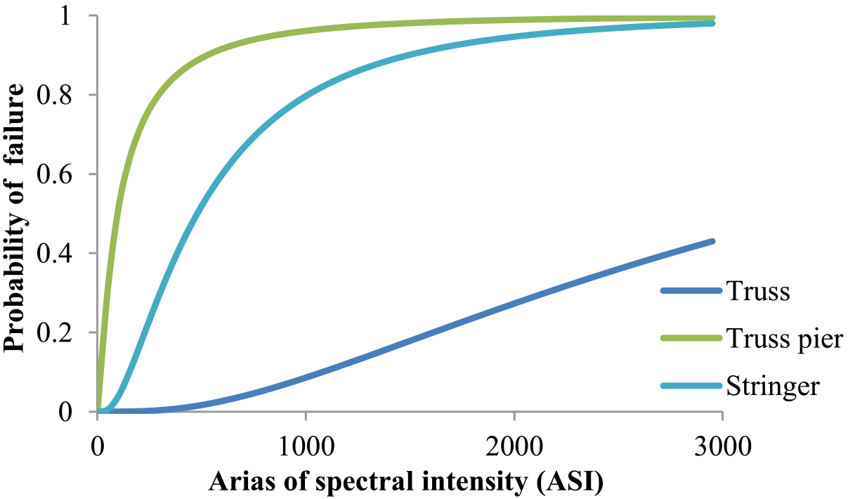
Element buckling capacities were calculated using AISC 360-2010 specifications, considering axial forces and moments acting on the bridge components, and were used to specify whether damage occurred to the component. Component fragility curves were derived based on the two-parameter log-normal distribution, as shown in Fig. 9.

Figure 7 Probability of Exceeding/ASI.

Figure 8 Probability of Exceeding/PGA.

Truss piers are the most vulnerable bridge elements. There are 5 piers in the Alasehir bridge, from 12–40 m long and constituted of steel truss elements, i.e., truss pier elements are slender and have relatively low buckling capacities. On the other hand, bridge superstructures are the safest components, with significantly lower buckling probabilities. Seismic risk analysis is required to obtain more information about overall bridge reliability.

Figure 9 Component fragility.

The entire bridge fragility was derived using a joint probabilistic seismic demand model (JPSDM) and limit state models. Demands for all components were generated using Monte Carlo simulation (10⁶ samples), based on the PDSM median and standard deviation, with fragility curve calculated from Eq. (6).

Bridge overall fragility was also calculated from the system upper and lower bounds. For a serial system, the bounds can be expressed as

$$\begin{array}{}\text{(8)}& {\displaystyle }{\displaystyle }\underset{i=\mathrm{1}}{\overset{n}{max}}\left[P\left(F_i\right)\right]\le P\left(F_{\mathrm{system}}\right)\le \mathrm{1}-\prod _{i=\mathrm{1}}^m\left[\mathrm{1}-P\left(F_i\right)\right],\end{array}$$

where P(F_i) is the failure probability of component i, and P(F_system) is the failure probability of the system. Maximum of component failure probability provides the lower bound (Nielson and DesRoches, 2007). Since there is some correlation between component demands, this provides a non-conservative result. In contrast, the upper bound assumes no component correlation and hence provides a conservative result. The actual system fragility curve is expected to lie between the upper and lower bound curves. If only one component significantly affects system fragility, the bounds become close, whereas if many components affect the system, the bounds can become wider (Nielson and DesRoches, 2007). Figure 10 shows the upper and lower bound, and the final Alasehir bridge fragility curves.

Figure 10 Bridge fragility and upper and lower bounds.

7 Conclusions

This study presents a seismic assessment of multi-span steel railway bridges in the Turkish railway system. The main concept was to determine bridge seismic behavior and safety under seismic conditions. Bridge PSDMs were obtained for the example the Alasehir bridge from 60 nonlinear time history analyses, and bridge component demands were used to derive component and overall bridge fragility curves.

Several IMs were considered to characterize the seismic event, and their relative practicality, efficiency, and proficiency was compared. Calculated fundamental period of Alasehir bride was obtained 0.38 and 0.59 s at x and y direction, respectively. Therefore, the fixed period S_a−0.2 s and S_a−1.0 s were not appropriate with fundamental period of the bridge. PGA, used frequently to derive bridge fragility curve, was also measured and reasonable results were achieved. β_EDP|IM was obtained in this study for PGA was similar with MSSS steel bridge. ASI was the most efficient practical and proficient for IM.

Alaşehir bridge fragility curves were derived for serviceability (from EN 1990 Annex 2) and component capacity limits. Velocity limits were shown to have important effects on the bridge fragility curve, with the bridge being significantly more vulnerable if the velocity limit exceeded 200 km h⁻¹. Thus, we propose that velocity limits for the Alaşehir bridge must be reduced. Median values for V > 200 km h⁻¹ serviceability fragility of Alaşehir bridge and slight damage fragility of MSSS steel bridge gave similar result. Moreover, fragility value refers to 10 % probability of exceeding in 50 year earthquake for 200 > V > 120 km h⁻¹ for serviceability limit state and slight damage for MSSS steel bridge demonstrated similar results. This means that Alaşehir bridge satisfies same performance with MSSS steel bridge for 200 > V > 120 km h⁻¹ serves velocity.

Component and system fragility curves were derived considering individual element buckling and fracture capacities. Truss piers elements were identified as the most vulnerable bridge components, whereas superstructure elements were the safest. Since truss piers significantly affect fragility, the system upper and lower fragility bounds were very narrow, and the overall bridge fragility curve was close to the lower bound, showing good correlation between component demands. Component fragility curve gave information about the individual performance of bridge component. Retrofitting strategy could be illustrated considering the most fragile component. Truss piers elements were critical components in the bridge and strongly affected the system fragility curve. System fragility curve derived using Monte Carlo simulation was between upper and lower bound.