the Creative Commons Attribution 3.0 License.
the Creative Commons Attribution 3.0 License.
Assessment of liquefaction-induced hazards using Bayesian networks based on standard penetration test data
Xiao-Wei Tang
Xu Bai
Ji-Lei Hu
Jiang-Nan Qiu
Liquefaction-induced hazards such as sand boils, ground cracks, settlement, and lateral spreading are responsible for considerable damage to engineering structures during major earthquakes. Presently, there is no effective empirical approach that can assess different liquefaction-induced hazards in one model. This is because of the uncertainties and complexity of the factors related to seismic liquefaction and liquefaction-induced hazards. In this study, Bayesian networks (BNs) are used to integrate multiple factors related to seismic liquefaction, sand boils, ground cracks, settlement, and lateral spreading into a model based on standard penetration test data. The constructed BN model can assess four different liquefaction-induced hazards together. In a case study, the BN method outperforms an artificial neural network and Ishihara and Yoshimine's simplified method in terms of accuracy, Brier score, recall, precision, and area under the curve (AUC) of the receiver operating characteristic (ROC). This demonstrates that the BN method is a good alternative tool for the risk assessment of liquefaction-induced hazards. Furthermore, the performance of the BN model in estimating liquefaction-induced hazards in Japan's 2011 Tōhoku earthquake confirms its correctness and reliability compared with the liquefaction potential index approach. The proposed BN model can also predict whether the soil becomes liquefied after an earthquake and can deduce the chain reaction process of liquefaction-induced hazards and perform backward reasoning. The assessment results from the proposed model provide informative guidelines for decision-makers to detect the damage state of a field following liquefaction.
- Article
(3991 KB) - Full-text XML
- BibTeX
- EndNote


The prediction of liquefaction potential (LP) and assessment of liquefaction-induced hazards are two significant and closely related problems. The former aims to determine whether the soil becomes liquefied after an earthquake, whereas the latter needs to not only predict whether liquefaction-induced hazards occur after soil liquefaction but also assess the severity of different hazards induced by liquefaction. The prediction of LP in foundation soils is only the first step in assessing liquefaction hazards. This has been well studied in recent decades, such as by simplified methods (Seed and Idriss, 1971, 1982; Starks and Olsen, 1995; Stokoe and Nazarian, 1985) based on standard penetration test (SPT), cone penetration test (CPT), and shear wave velocity measurements, laboratory testing, numerical methods, and empirical liquefaction models (Goh, 1994; Zhang and Goh, 2013, 2016; Pal, 2006; Toprak et al., 1999; Zhang et al., 2015) based on historical data. What is more important to engineers is the effect of liquefaction-induced hazards on foundations or superstructures after seismic liquefaction, although relatively few studies have focused on this issue (Juang et al., 2005).
Field evidence of liquefaction-induced hazards during historical earthquakes mainly consists of sand boils (SB), ground cracks (GC), the settlement and tilting of structures, and lateral spreading (LS) failures. Several methods have been proposed to quantify these hazards, including numerical simulations, laboratory tests, and field testing. Although recent advances in physical model experiments and the computational modelling of liquefaction-induced ground deformation are quite promising, there are some critical unresolved problems. For instance, without a perfect physical numerical model for totally describing the complicated mechanic characteristics of soils, it is expensive and difficult to obtain and test high-quality undisturbed samples of loose sandy soils. Therefore, empirical liquefaction models based on historical earthquake databases are best suited to providing a simple, reliable, and direct means of assessing liquefaction-induced hazards in the field of geotechnical earthquake engineering (Zhang et al., 2002). In terms of empirical liquefaction methods, the liquefaction potential index (LPI) has been used to characterize liquefaction-induced hazards worldwide (Iwasaki et al., 1982). Several subsequent approaches built on the LPI, such as the damage severity index (DSI) (Juang et al., 2005), the Ishihara-inspired LPIISH (Maurer et al., 2015), and the liquefaction severity number (LSN) (Tonkin & Taylor Ltd., 2013). In addition, generalized analytical or empirical techniques for estimating a single type of ground failure (e.g. settlement or lateral spreading) induced by liquefaction have been proposed in recent decades (Youd and Perkins, 1987; Youd et al., 2002; Goh and Zhang, 2014; Ishihara and Yoshimine, 1992; Zhang et al., 2002; Wu and Seed, 2004; Cetin et al., 2009; Juang et al., 2013). With the rapid development of computer technology and mathematical techniques, many new artificial intelligence methods for assessing liquefaction-induced ground deformation have been developed based on historical data (Wang and Rahman, 1999; Baziar and Ghorbani, 2005; Javadi et al., 2006; Garcia et al., 2008; Rezania et al., 2011). However, the assessment of liquefaction-induced hazards is a complex engineering problem because of the heterogeneous nature of soils, a large number of factors involved, and the uncertainties associated with these factors. The existing methods were either developed statistically or could only assess one type of hazards, such as settlement or lateral spreading. Additionally, they do not consider the effects of uncertainties on the model performance, especially the purely data-driven approaches, which ignore the effects of empirical knowledge or domain knowledge on the assessment of liquefaction-induced hazards. Because there is no generic model for calculating or assessing sand boils, ground cracks, lateral spreading, and settlement simultaneously and then evaluating the overall severity of hazards induced by liquefaction after an earthquake, it is necessary to develop a framework for assessing all types of liquefaction-induced hazards at a given site following an earthquake. The latest developments in BN technology provide new opportunities to develop better tools for complex problems in probabilistic terms, such as the problem of liquefaction-induced hazards. The primary objective of this paper is to use Bayesian network (BN) methods to integrate soil liquefaction, LPI, the four types of hazards (ground cracks, sand boils, lateral spreading, and settlement) induced by liquefaction, and the severity of liquefaction-induced hazards (SLH, describing the overall situation of a site) into one model based on historical SPT data. This would allow us to deduce the chain reaction process of hazards, from an earthquake event to seismic liquefaction to liquefaction-induced hazards, thus enhancing the existing simplified methods that only assess one single liquefaction-induced hazard. The BN model is trained and tested separately using two different real-world datasets. The results given by the BN model for the evaluation of liquefaction-induced hazards are compared with those from an artificial neural network (ANN) model to verify the effectiveness and robustness of the proposed approach. Afterward, the BN model is applied to evaluate the hazards induced by liquefaction during the 2011 Tōhoku earthquake in Japan.
2.1 Why Bayesian network?
BNs are one of the most effective theoretical models for knowledge representation and reasoning under the influence of uncertainty and highly non-linear relationships among variables (Pearl, 1988). Firstly, BNs offer a rational and coherent theory under the condition of various uncertainties (e.g. uncertainties in parameters, models, and domain knowledge) and complexities that are described in terms of subjective beliefs or probabilities to reflect the interdependent relationship between variables. Moreover, they can integrate different types of domain knowledge and multi-source information or various quantitative and qualitative factors into a consistent system and facilitate multiple hazards and their interdependencies within a single model. In particular, this allows not only sequential inference (from causes to results) but also reverse inference (from results to causes) under conditions of complete and even incomplete data and provides an efficient framework for the probabilistic updating and assessment of component performance when new evidence emerges.
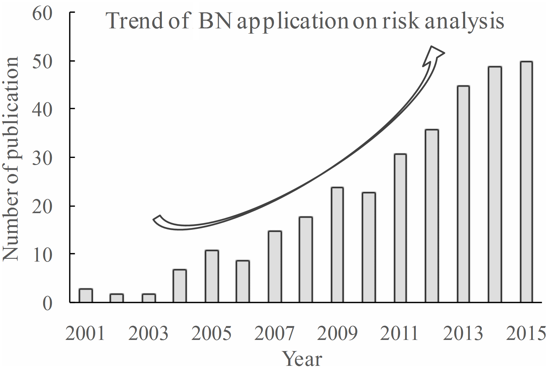
In recent decades, BNs have been widely applied for risk analysis in the field of engineering, such as for catastrophic risk (Li et al., 2010a, b, 2012), earthquake risk damage (Bayraktarli et al., 2005; Bayraktarli and Faber, 2011; Bensi et al., 2009, 2014), embankment dam risk (Zhang et al., 2011; Xu et al., 2011; Peng and Zhang, 2012), landslide hazards (Song et al., 2012; Liang et al., 2012), and soil liquefaction (Bayraktarli, 2006; Hu et al., 2015). However, the application of BNs in assessing liquefaction-induced damage has never been reported. An important sign is that the number of relevant publications in this field over the period 2001–2015 (obtained by querying “BN” and “risk analysis” in the Web of Science database) increased from 3 to 50 (as shown in Fig. 1). In the past 5 years, BN technology has become popular with engineers and researchers for the assessment of risk. BN techniques are known to be a robust method for risk analysis.
2.2 Probabilistic reasoning of BNs
BNs combine graph theory and statistics using arcs or links with conditional probabilities. The inference algorithms are based on the Bayesian rule, chain rule, and conditional independence rule as follows:
where P(Y) is the prior probability, P(X|Y) is one's belief in hypothesis X upon observing evidence Y, which is known as the posterior probability, and P(Y|X) is the likelihood that Y is observed if X is true. π(xi) is a set of values for the parents of Xi.
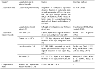
Table 1Factors of liquefaction and its induced hazards and empirical modelling methods.
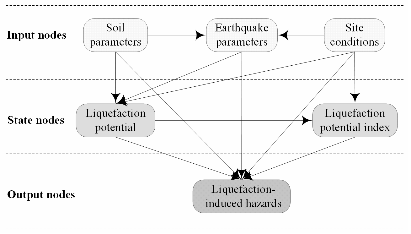
A generic BN model for liquefaction-induced hazards (as shown in Fig. 2) is constructed with domain knowledge to illustrate how to reason in the assessment of liquefaction-induced hazards. There are three types of nodes in the BN model: (1) input nodes, i.e. soil parameters (SP), earthquake parameters (EP), and site conditions (SC), which are factors in seismic liquefaction; (2) state nodes, i.e. LP and LPI, which show whether the soil is liquefied and express the degree of soil liquefaction, respectively; and (3) output nodes, i.e. liquefaction-induced hazards, such as lateral spreading, settlement, ground cracks, and sand boils, which express the SLH. The nodes are connected by 12 arcs or links. In the risk assessment of liquefaction-induced hazards, if evidence comes from input nodes, the posteriori probability or belief that the target variable (liquefaction-induced hazards, here LH) is in a certain state (e.g. severe) can be derived by the following formulas:
2.3 Construction of a BN model for liquefaction-induced hazards
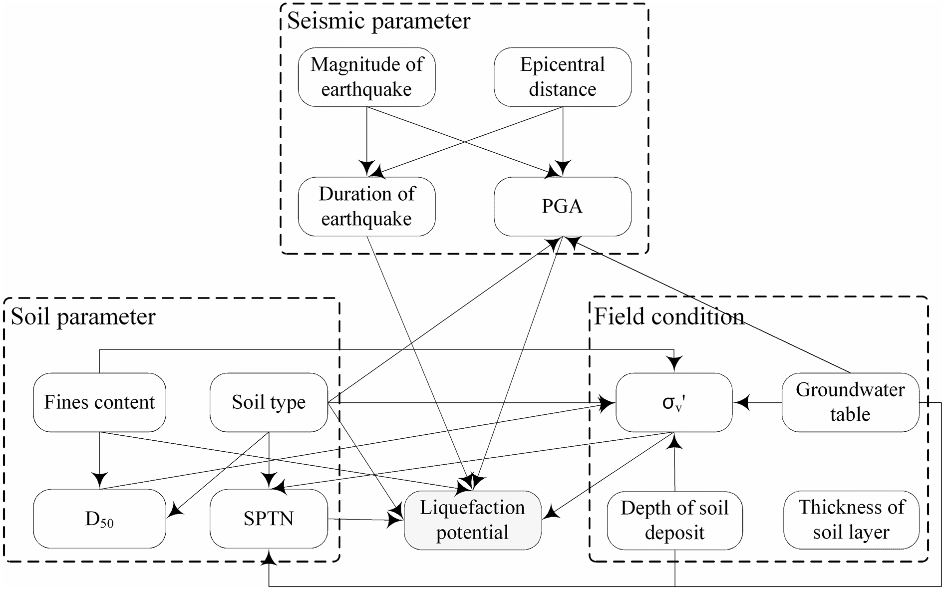
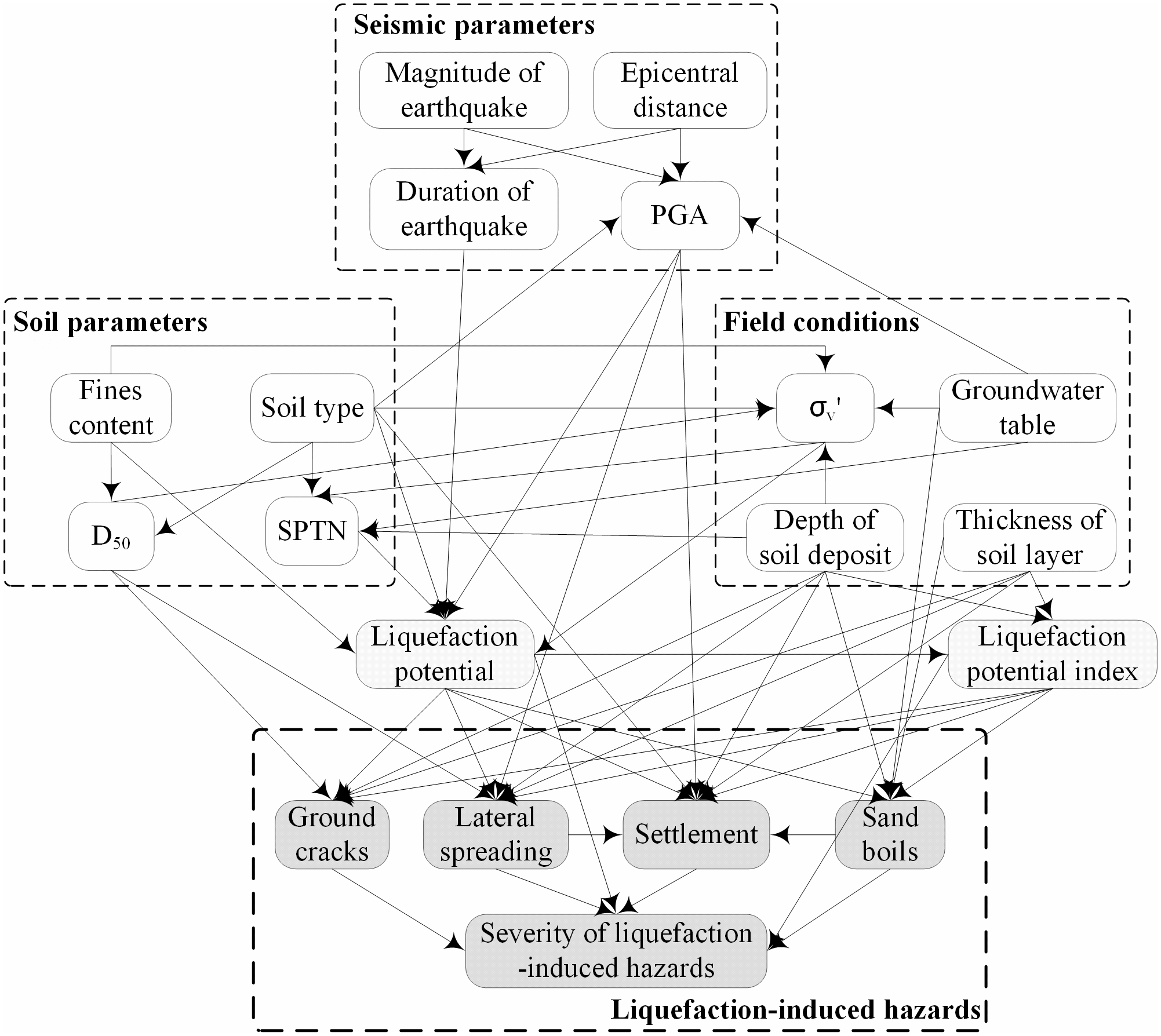
Strong earthquakes can cause liquefaction and therewith ground failures in the form of sand boils, ground cracks, settlement-induced tilting of structures, and lateral spreading. Table 1 lists some factors related to the LP, LPI, four types of hazards induced by liquefaction, and SLH. LP and LPI are used to describe the state of soil liquefaction, the four types of liquefaction-induced hazards are used to identify different types of damage and their severity after seismic liquefaction, and SLH is a comprehensive index intergrading indexes of the four types of hazards to describe the overall severity of disasters after liquefaction. Additionally, Table 1 lists some empirical modelling methods that can be used as domain knowledge to construct a BN model of liquefaction-induced hazards. Hu et al. (2016) constructed a BN model for liquefaction potential (as shown in Fig. 3) that considered 12 factors: the magnitude of the earthquake (ME), epicentral distance (ED), duration of the earthquake (DE), peak ground acceleration (PGA), fine content (FC), soil type (ST), average particle size (D50), SPT number (SPTN), vertical effective stress (), groundwater table (GT), depth of soil deposit (DSD), and the thickness of the soil layer (TSL). In terms of seismic parameters, the liquefaction potential will increase with increases in ME, DE, and PGA and lower values of ED. In terms of soil parameters, the anti-liquefaction behaviour of the soil is strongly related to the FC value: as FC increases up to 30 %, the liquefaction strength decreases, but when FC exceeds 30 %, the liquefaction strength increases with FC; when FC > 50 % (silt and sandy silt), the soil is hardly liquefied. In addition, the FC value determines the type of soil. Normally, purified clay and silt cannot be liquefied, whereas poorly graded sand and silty sand are easily liquefied. The bigger the average particle size, and the bigger the SPTN, the smaller the probability of soil liquefaction. In terms of field conditions, deeper soil deposits have greater vertical effective stress. This is more difficult for the increase in pore water pressure to overcome, so soil liquefaction cannot easily occur. In addition, a shallow GT and thin soil can partly reduce the probability of soil liquefaction. Thus, a state node (LPI) and output nodes (sand boils, ground cracks, lateral spreading, settlement, and SLH) should be added to the existing BN model of liquefaction potential (shown in Fig. 3) based on the generic BN model in Fig. 2. A new BN model for liquefaction-induced hazards (shown in Fig. 4) was constructed according to domain knowledge of the hazards in Table 1. The ground slope, which affects GC and LS, was not considered in the BN model of liquefaction-induced hazards because associated data were not collected in the present study.
Earthquake liquefaction-induced hazards are a chain reaction, originating with the earthquake event and proceeding to soil liquefaction and its pertinent hazards. Different input values result in different liquefaction states and different degrees of liquefaction. The outputs of the former system (e.g. LP) are used as input information for the latter system, resulting in different hazard events (e.g. sand boils, lateral spreading). The whole process of earthquake liquefaction-induced hazards can be described as follows: at the beginning of an earthquake, the earthquake parameters, soil characteristics, and field conditions are considered as control variables, and their prior probabilities are calculated by parameter learning. The posterior probability of the output variable (e.g. LP) can then be inferred to estimate whether an event could be triggered. If the event occurs, its conditional probability is replaced by the posterior probability, which is considered as the evidence variable for input. Finally, a posterior probability of the latter event (e.g. LP) is calculated using the new conditional probability of the former event to estimate its grade. The above process is repeated until the grades of all hazard events have been identified.
3.1 Dataset
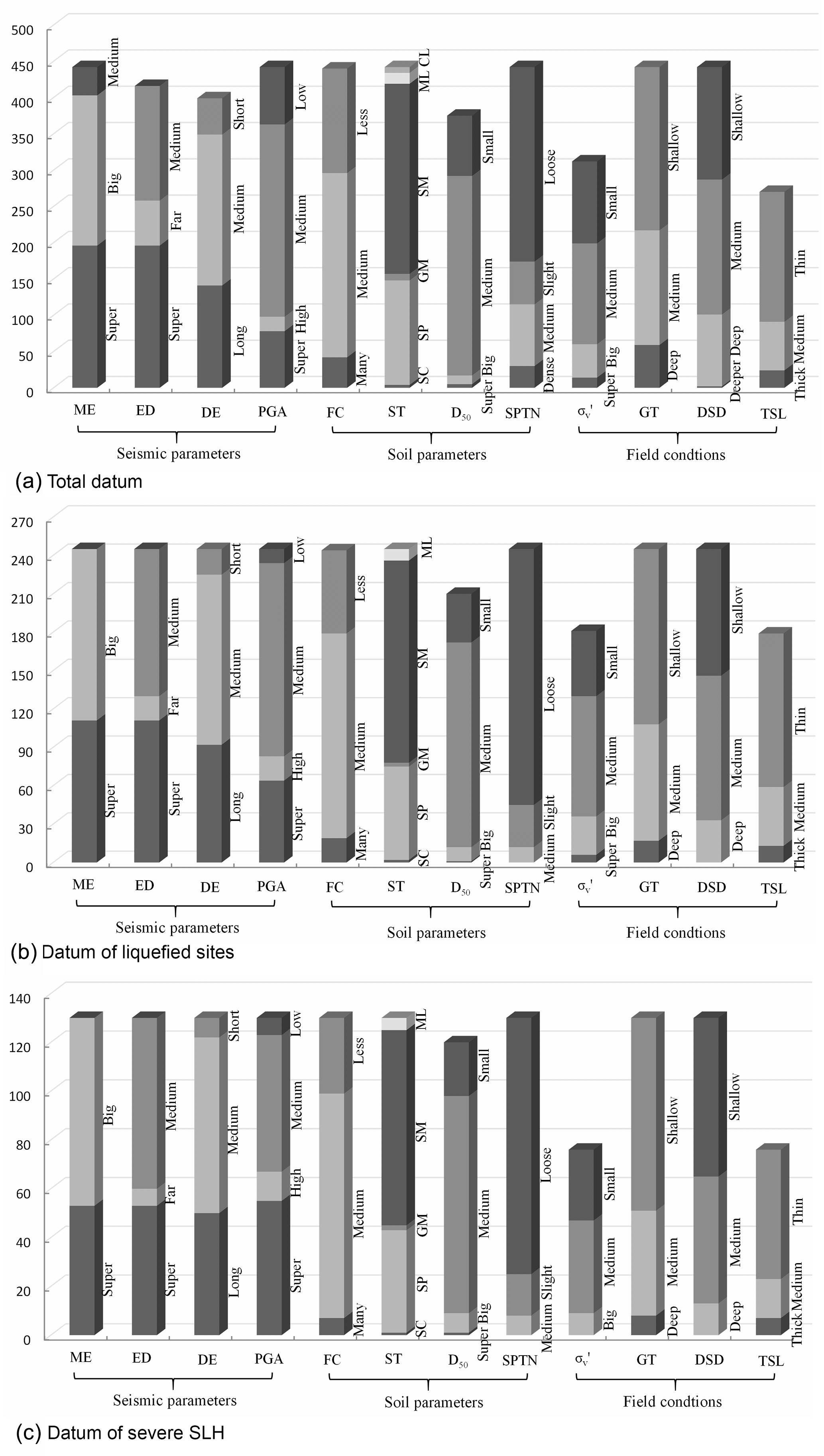
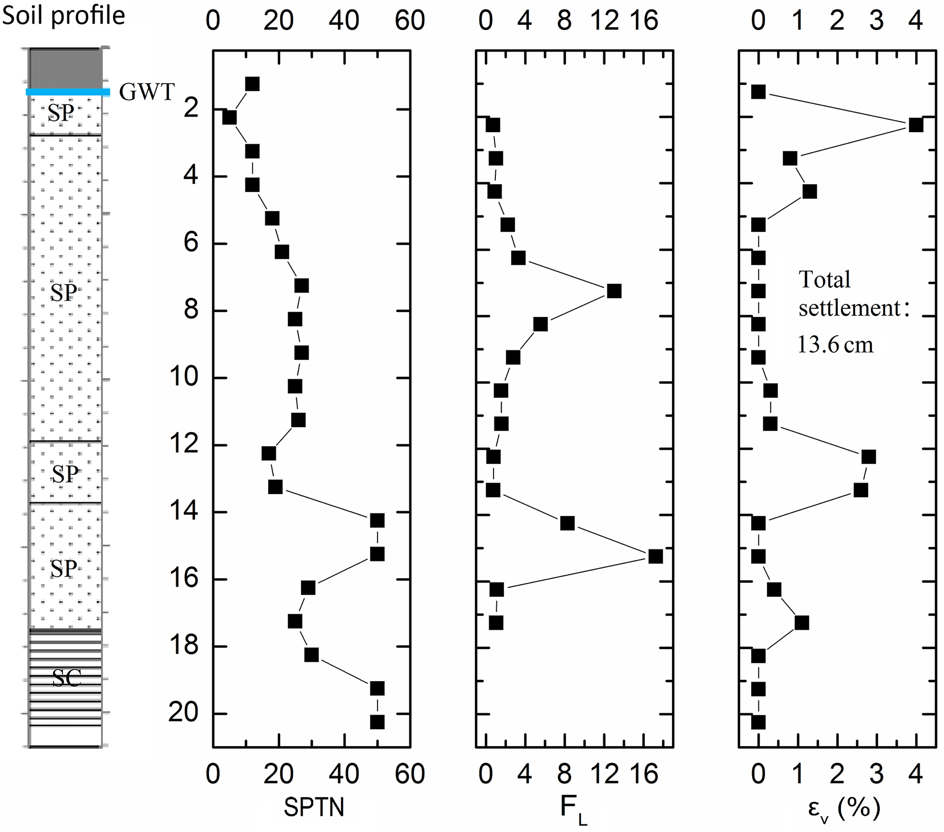
In this study, the dataset shown in Fig. 5a consists of 442 SPT borings from post-earthquake in situ tests at liquefied (245 SPT borings; shown in Fig. 5b) and non-liquefied (197 SPT borings) sites in Taiwan, Japan, and the USA. Of these, 332 SPT borings (184 liquefied sites and 148 non-liquefied sites) were used to train the BN model, and the remaining 110 SPT borings were used to test the effectiveness and robustness of the BN model. Only four earthquakes above are considered in this study, “medium magnitude” data from the 1957 Daly City (California, USA) earthquake (Mw=5.3) and the 1987 Whittier Narrows (USA) earthquake (Mw=5.9) were taken from Cetin et al. (2000). “Big magnitude” data from the 1999 Chi-Chi earthquake in Taiwan (Mw=7.6) were downloaded from http://www.ces.clemson.edu/chichi/TW-LIQ/In-situ-Test.htm (last access: 21 October 2016) and http://peer.berkeley.edu/lifelines/research_projects/3A02/ (last access: 21 October 2016). “Super magnitude” data from the 2011 Tōhoku earthquake in Japan (Mw=9.0) were provided by the Research Centre for the Management of Disasters and the Environment at Tokushima University, Japan. “Strong magnitude” (6Mw < 7) is not included. The collected data of these four earthquakes covers not only different duration and PGA but also several soil parameters and field conditions, none of which are located within 10 km (defined as “near” epicentral distances) from earthquake sources. The grading standard of all 12 influence factors of liquefaction potential in Fig. 5 is shown in Table 2, from Hu et al. (2016). The observed liquefaction effects induced by these earthquakes include sand boils, settlement of ground, ground cracks, and lateral spreading (as shown in Fig. 6), resulting in the destruction of cropland, blocking of channels, and severe damage or collapse of many buildings, highways, bridges, harbour facilities, and other infrastructure components.
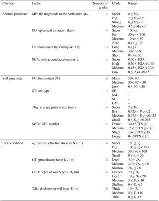
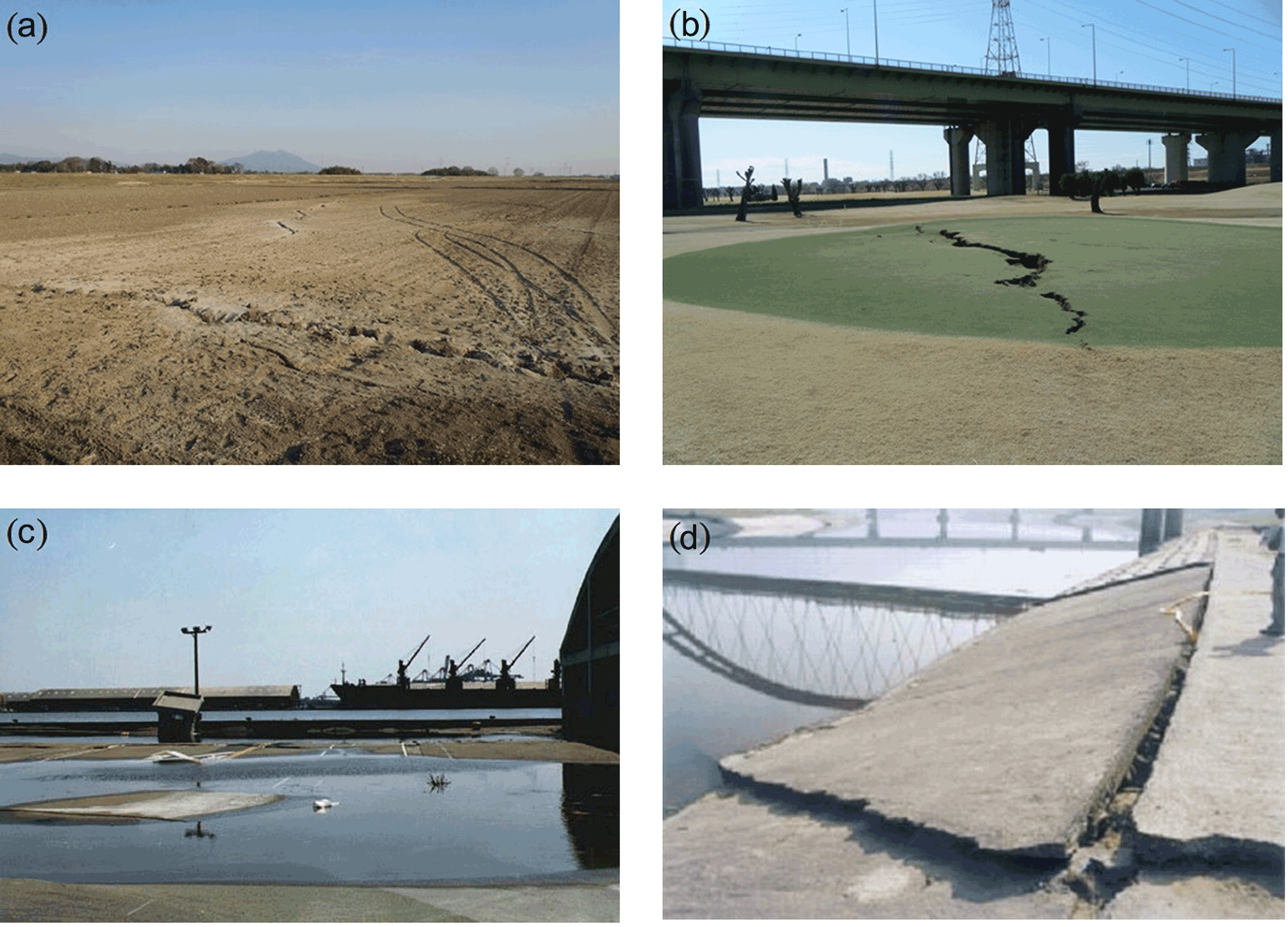
Figure 6Photos showing liquefaction-induced hazards during the Chi-Chi earthquake and the 2011 Tōhoku earthquake: (a) sand boils in Chikusei; (b) ground cracks at Arakawa River in Toda; (c) settlement at Taichung Port (http://www.ces.clemson.edu/chichi/TW-LIQ/Liq-Album/Settlement-7.htm, last access: 10 December 2016); (d) lateral spread induced failure of a dike in Nantou (http://www.ces.clemson.edu/chichi/TW-LIQ/Liq-Album/LatSpread-3.htm, last access: 10 December 2016). Images © 2016 Clemson University.
The liquefied sites of the collected data in this study are mainly from the Chi-Chi earthquake and Tōhoku earthquake. The characteristics of liquefied soils are predominantly loose and clean sands or silty sands (SPT values less than 10) that deposit within 10 m in the liquefaction data of the two earthquakes shown in Fig. 5b. It is worth noting that duration of ground motion was very long within 100–200 s, and the liquefied sites were very far from the epicentre of about 300–450 km, which experienced PGAs of approximately 150–300 cm s−2 during the Tōhoku earthquake, whereas serious damage induced by soil liquefaction occurred in a wide area of the Tōhoku and the Kanto regions along with a wide range of sand boils, cracks, and severe uneven settlement of pavements due to long-lasting cycle shear actions. However, during the Chi-Chi earthquake, durations of the strong motions were short, but PGA values were very big due to near a source earthquake proximal to a fault (approximately 1.0 km), e.g. in the Nantou and Wufeng regions as high as 0.7–1.0 g, that caused widespread liquefaction in the form of sand boils, lateral spreads, and settlement of grounds in the towns of Yuanlin, Nantou, and Wufeng, Taiwan. Figure 5c shows proportions of all influence factors for the severe status of the SLH. It is clear that the most severe damage sites were the result of big or super earthquakes (Mw > 7 or 8) with long loading (duration more than 60 s); some epicentral distances were close to the earthquake sources, e.g. the nearest liquefied sites in Nantou are about 14 km away from the epicentre, and thus their PGA was sufficiently high. As for soil characteristics, pure sand or silty sand with moderate fine content (30 % < FC ≤ 50 %) and moderate average grain diameter (0.075 ≤ D50 < 0.425) values result in severe damage, unlike sites with gravelly soil and sandy silt. The damage phenomena also indicate that, even though gravel and sandy silt are not easily liquefied when the earthquake is sufficiently strong to cause liquefaction, severe damage can be expected, as shown in Fig. 5b and c. The small SPTN (0 < SPTN ≤ 10) means that the sandy soil is so loose that settlement and lateral spreading are more likely triggered after liquefaction because loose sand is more easily compressed and flows during seismic liquefaction. As for field conditions, the shallow-buried sandy soil layer has low effective stress ( < 50 kpa) and the GT is near to the ground surface. Such zones are likely to suffer from severe damage. The above laws fit well with practical engineering experience. The sum of the data size of these 12 variables is not consistent in Fig. 5a, b, and c, respectively, such as ED, DE, D50, , and the TSL due to the missing data. The proportion of missing data for ED, DE, D50, vertical effective stress, and the thickness of soil layer is ∼ 5, ∼ 9.7, ∼ 15.2, ∼ 29.4, and ∼ 38.9 %, respectively. An expectation–maximization (EM) algorithm (Lauritzen, 1995) was used to train the 332 SPT data to obtain a conditional probability table for the BN model because of incomplete data. EM was used as it is more robust than other algorithms and is suitable for datasets with many missing values. Briefly, the EM method is an iterative algorithm for determining the maximum likelihood estimation or maximum a posteriori estimation of parameters. A Bayesian net is iteratively applied to obtain a better one by conducting an expectation (E) step followed by a maximization (M) step until the algorithm has converged. In the E step, the regular Bayesian net inference is used with the existing Bayesian net to compute the expected value of all the missing data, and then the M step finds the maximum likelihood Bayesian net, given the now extended data (e.g. original data plus expected values of missing data).
Table 3Grading standard for liquefaction and liquefaction-induced hazards.
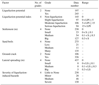
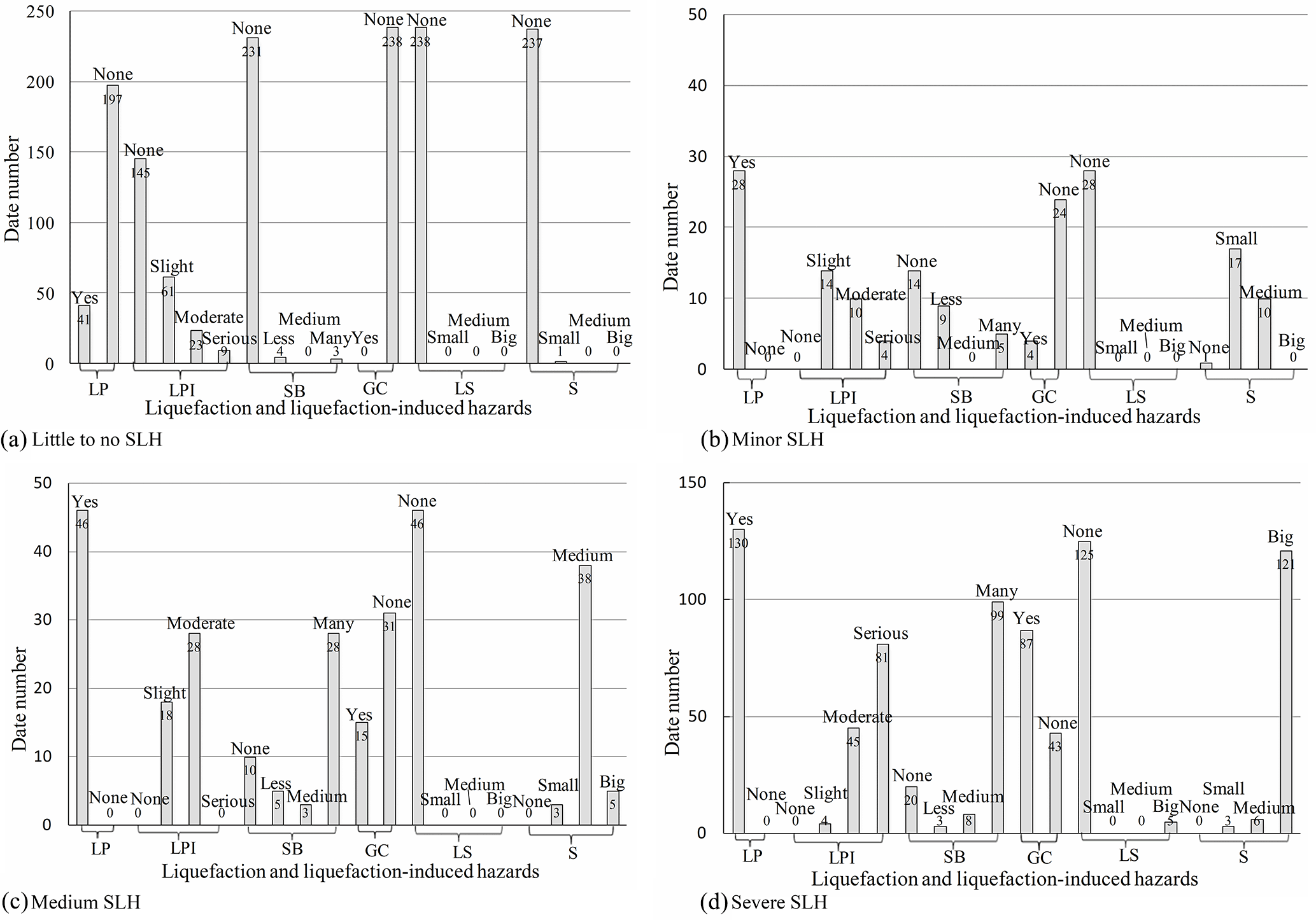
Table 4Description of the severity of liquefaction-induced hazards.
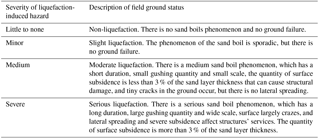
The grading standard of liquefaction potential index and liquefaction-induced hazards according to domain knowledge is presented in Table 3; e.g. LPI is divided into four grades according to Iwasaki et al. (1982): non-liquefaction (LPI = 0), slight liquefaction (0 < LPI ≤ 5), moderate liquefaction (5 < LPI ≤ 15), and serious liquefaction (LPI > 15). SLH is divided into four grades according to disaster experience in the field of engineering, as described in Table 4. According to the descriptions of SLH, a statistical summary of liquefaction-induced hazard data is presented in Fig. 7. It can be seen that (1) liquefaction does not have to induce hazards, but the occurrence of liquefaction-induced hazards is based on liquefaction. (2) LPI is not a good index for describing the severity of liquefaction-induced hazards because the efficacy of the LPI framework and accuracy of derivative liquefaction hazards are uncertain; e.g. serious liquefaction according to LPI occurs in the absence of SLH (see Fig. 7a) and slight liquefaction according to LPI occurs when severe SLH are observed (see Fig. 7d). As a rule, the bigger the LPI, the greater the severity of the corresponding liquefaction-induced hazards. (3) SB, S, GC, and LS are macroscopic phenomena of liquefaction-induced hazards, and there is a trend that the bigger the values of these indexes are, the more severe the SLH. (4) The classifications for the four different types of hazards in Fig. 6 almost accord with the descriptions of the field ground damage status in Table 4.
3.2 Performance indexes
In this section, to comprehensively evaluate the performances of the two probabilistic models for liquefaction-induced hazards, several performance indexes are introduced. These are the accuracy, prediction, recall, area under the curve (AUC) of the receiver operating characteristic (ROC), and Brier score. The details of these indexes are described in the following.
The accuracy is a measure of the percentage of correctly classified instances for each class. This metric is widely used for measuring the overall performance of a classifier. For instance, an accuracy of 0.9 indicates that 90 % of the data can be correctly classified. However, it does not mean that the accuracy of each class is 90 %; the accuracy of one class may be high, whereas that of the others may be very low. Therefore, evaluations of predictive capability based on accuracy alone can be misleading when a class imbalance exists in a dataset. Indexes such as the precision, recall, and AUC of ROC should be used to further measure the performance of each class for a model or classifier.
The recall refers to the probability of detection of a class and measures the proportion of correctly predicted positive instances among all actual positive cases. If a classifier can achieve a higher recall for a class, then it can detect more positive instances of the class. The precision refers to the proportion of true positives among the instances predicted as positive for a single class, but it cannot measure how the classifier detects the actual positive instances. A classifier with high precision but lower recall is less useful because it cannot detect significant positive instances, especially in terms of risk assessment, where security and warning are major concerns. A good classifier should detect more positive instances with relatively high prediction accuracy and have high recall and acceptable precision.
The ROC curve is a graphical plot given by the false positive rate (the proportion of all negatives that still yield positive test outcomes) on the x axis and the true positive rate or recall on the y axis, which can present an overly optimistic view of an algorithm's performance. The AUC of ROC is the area between the horizontal axis and the ROC curve, which is a comprehensive scalar value representing a classifier's expected performance. The AUC of ROC ranges from 0.5 to 1, with values closer to 1.0 indicating better precision. Therefore, the bigger the AUC of ROC value, the better the prediction performance of the classifier.
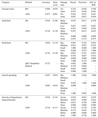
Table 5Comparison of predictive performance of liquefaction-induced hazards.
The Brier score (Brier, 1950) is used to measure the quality of probabilistic forecasts for discrete events. Suppose that on each of n occasions, an event can occur in only one of r possible classes. On the ith occasion, the forecast probabilities that the event will occur in classes are , respectively. The Brier score (B) is then defined by
where , . Eij takes a value of 1 or 0 according to whether the event occurred in class j or not. For instance, in the case study described in this paper, 110 SPT borings are used for testing (n=110), SLH has four classes (none, minor, medium, and severe; r=4), and a probability or confidence statement (fij) is given for each SPT boring instance. The Brier score ranges from 0 to 2, where B=0 denotes a perfect prediction and B=2 denotes the worst possible prediction.
4.1 Comparison of predictive results
Table 5 compares the predictive results given by the BN model (see Fig. 4) and the ANN model using the same parameters. In terms of accuracy, except for LS, the BN model scores higher than the ANN model for the other types of hazards and SLH and comparing the Brier score, the BN model scores lower than the ANN, except for LS and SLH. These results indicate that the overall performance of the BN model is better than that of the ANN model. As for each type of hazard induced by liquefaction and SLH, the recall, precision, and AUC of ROC scores obtained by the BN model for each class are generally higher than those of the ANN, which also suggests that the BN model is better than the ANN model. Therefore, the proposed BN approach is better than the ANN technology, and its performance is acceptable for monitoring and forecasting seismic liquefaction-induced hazards. In addition, in terms of the computation time, the BN model (using the EM algorithm) outperforms the ANN model (containing 20 hidden layers and using a radial basis function), requiring 36 iterations (about 19.8 CPU s) to converge to a stable state. This convergence rate is faster than that of the ANN model.
Furthermore, there are no effective simplified methods for estimating ground cracks and sand boils, and simplified methods for calculating lateral spreading (Bartlett and Youd, 1995; Wang and Rahman, 1999; Goh and Zhang, 2014) require the free face ratio or ground slope, which were not included in the data collected for this study. Therefore, ground cracks, sand boils, and lateral spreading cannot be estimated by simplified methods. However, settlement can be calculated by the simplified method proposed by Ishihara and Yoshimine (1992), hereafter referred to as the I&Y method. Table 5 clearly indicates that the predictive results of data-driven methods such as BN and ANN are better than those of the simplified I&Y method, but the simplified approach gives a constant value (as shown in Fig. 8) rather than an interval value or probability. In addition, the simplified method is constructed using only the relationships among the relative density, the factor of safety against liquefaction (FL), and the volumetric strain (εv). The factor of safety against liquefaction is obtained by integrating the earthquake intensity and SPTN using empirical formulas or empirical coefficients and thus may introduce calculation errors that result in considerable prediction errors, such as the small settlement predicted in Table 5, where the precision of the simplified method is only 0.069. However, the data-driven methods integrate multiple factors of liquefaction-induced hazards into a model, thus providing better predictive performance than the simplified method.
4.2 Causal reasoning using the BN model
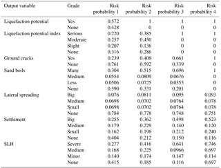
Based on the developed BN model, the probabilities of the liquefaction-induced hazards were inferred through causal reasoning. The third column in Table 6 lists the posterior probabilities of all grades of LP, LPI, and its induced hazards. It can be seen that when the input variables regarding earthquake parameters, soil characteristics, and field conditions are unknown, the probabilities of all grades of each output variable are similar, except for LS and SB, which have a serious imbalance in the data of different grades. However, when a site is determined to be liquefied and the probability of a positive LP status becomes 100 %, the fourth column shows that the probabilities of LPI being “none” and all hazards decrease to some extent while the probabilities of other LPI states and all hazards increase significantly. Furthermore, if the site is seriously liquefied, the probability of LP being “yes” and LPI being “serious” becomes 100 %, as seen in the fifth column of Table 6. The probabilities of all grades (except “none”) for all hazards continue increasing, with GC occurring with 66.1 % probability, serious sand boils occurring with 69.6 % probability, big LS occurring with 9.5 % probability, big settlement occurring with 49.8 % probability, and severe SLH occurring with 64.1 % probability. This shows that liquefaction-induced hazards are much more severe at seriously liquefied sites. Macro-liquefaction phenomena, such as GC and serious SB, are also observed, and the probabilities of the “big” status in other hazards continue to increase slightly, as seen in the sixth column of Table 6. Thus, the predictive results are close to the actual situation. Therefore, according to the above deduction process, the BN model can calculate the posterior probability of LP based on the conditional probabilities of input variables for estimating whether a site is liquefied or not. If it is liquefied, its posterior probability will be considered as input information for predicting the latter variable. Such reasoning gives all predictive results of liquefaction-induced hazards. In addition, when the prior probabilities of all input variables, such as the earthquake parameters, soil characteristics, and field conditions, have been determined in advance, the predictive performance for all hazards will improve significantly. For instance, consider a site that suffered a long-duration super earthquake. Surveys show that the SLH is severe with a big settlement, no lateral spreading, serious sand boils, and ground cracks. The input variables of the site indicate that the ED is near, the PGA is higher, the SE is sand with some fine particles, the D50 value is medium, the sand is loose according to the SPTN, the value is small, the GT is shallow, and both the depth and thickness of the sand layer are moderate. The reasoning probability value of LP is 99.9 %, LPI is identified as serious with 43.8 % probability, and GC has a 51.4 % probability of not occurring, which does not match the survey results. According to the input information, SB is identified as “many” with 76.5 % probability, LS is identified as “none” with 85.0 % probability, the settlement is identified as “big” with 53.1 % probability, and SLH is identified as “severe” with 52.6 % probability. The site is then determined to be a liquefied area with serious liquefaction degree, so LP should be 100 % and the probability of LPI being serious should also be 100 %. The probabilities of all hazards will also change. GC occurs with 100 % probability, which matches the survey results; LS is identified as “none” with 100 % probability (an increase of 15 %); settlement is identified as “big” with 100 % probability (an increase of 46.9 %); and SLH is identified as “severe” with 100 % probability (an increase of 47.4 %).
Table 7Most probable explanation of LP, serious LPI, GC, many SB, big LS, and big S in the BN model.
4.3 Diagnostic reasoning using the BN model
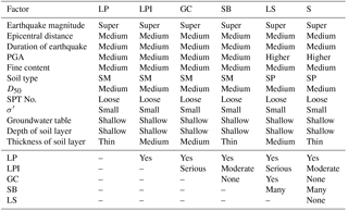
To detect situations that are more likely to result in severe damage, the most probable explanations of LP (yes), LPI (serious), GC (yes), SB (many), LS (big), and S (big) are inferred using the diagnostic reasoning capabilities of the BN model. The results are presented in Table 7. It can be seen that loose silty sand (medium D50) containing moderately fine particles deposited shallowly (small ) on a site with a low underground water level is more likely to suffer from liquefaction following a super earthquake of moderate duration and moderate epicentral distance. The most probable explanations for GC and “many” SB are the same as those for LP under conditions of serious or moderate soil liquefaction, but the most probable explanations for “big” LS and “big” S are slightly different from those of LP in terms of PGA and SE. The reason is that both LS and S being “big” requires more seismic intensity than occurrences of sand boils and ground cracks, and sand flows more easily and undergoes greater compression after liquefaction than sand containing fine particles. In addition, LS and S being “big” is often accompanied by many sand boils, whereas ground cracks may or may not occur. The above results agree with the analysis results in Fig. 7. In addition, if the soil characteristics, field conditions, and hazards are known, the earthquake intensity (ME, DE, PGA, and ED) resulting in liquefaction-induced hazards can be estimated using the backward inference ability of the BN method, which provides some references for aseismatic design.
4.4 Sensitivity analysis of liquefaction-induced hazards
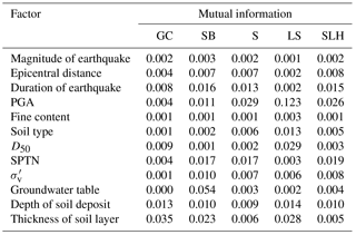
Sensitivity analysis detects how much each factor impacts the target variable. In this section, mutual information is used to assess the sensibility, which is a measure of the mutual dependence between two variables. The mutual information results for different liquefaction-induced hazards were computed separately in the BN model; the results are presented in Table 8. The TSL is the most sensitive variable for GC, and the relatively important factors are the depth of the soil layer, D50, and the DE. For SB, the GT is the most sensitive variable, and the relatively important factors are the TSL, SPTN, DE, PGA, depth of soil layer, and . For S, PGA is the most sensitive variable, and the relatively important factors are SPTN, the DE, and the depth of the soil layer. For LS, PGA is again the most sensitive variable, and the relatively important factors are D50, the TSL, the depth of the soil layer, and the soil type. These results are highly consistent with the domain knowledge in Table 1. Comparing the most sensitive factors and relatively important factors of the four types of liquefaction-induced hazards and SLH, the DE, PGA, SPTN, DSD, and the TSL are more important than the other factors because they are present for more than three items; the findings are in agreement with the description of characteristics of earthquake- and soil-induced liquefaction hazards in Sect. 3.1. For these five factors, a combination of SPTN and the earthquake intensity (described by the DE and PGA) can detect the degree of soil liquefaction. The depth of the soil deposit and the TSL combine with the relative density (determined by SPTN) based on the degree of soil liquefaction to give the soil volumetric strain. Consequently, liquefaction-induced hazards, e.g. settlement and lateral spreading, can be estimated. Therefore, to mitigate seismic liquefaction-induced hazards, we can neglect the relative density of sandy soil, as the depth of the sandy soil deposit and the thickness of the sandy soil layer are the crucial factors.
Table 8Sensitivity analysis of seismic liquefaction-induced hazards.
The BN model described above was applied to assess the liquefaction-induced hazards during Japan's Tōhoku earthquake on 11 March 2011. The research regions are Ibaraki Prefecture, Chiba Prefecture, Saitama Prefecture, Kanagawa Prefecture, and Tokyo, which contain 196 investigation sites. In the 196 real fields, the prediction accuracies of the four types of liquefaction-induced hazards are 99.50 % (lateral spreading), 81.63 % (sand boils), 80.61 % (settlement), 89.8 % (ground cracks), and 84.1 % (SLH). In addition, the prediction accuracies of the four different levels of SLH (little to none, minor, medium, and severe) are 79.83, 84.62, 81.25, and 79.83 %, respectively, which demonstrate the validity of the BN model in general. The prediction accuracies of the LPI approach (Iwasaki et al., 1982) for the four different levels of SLH were found to be 36.96, 8.82, 68, and 42.22 %, respectively, which are much worse than the prediction results of the BN model.
During this earthquake, areas with greater losses and a larger number of liquefaction sites are located in Ibaraki Prefecture and Tokyo, which are closer to the sea than the other places. These two regions contain 78 sites with different degrees of hazards, including approximately 50 sites where medium or severe disasters occurred. In Table 4, it is apparent that sites suffering medium or severe disasters were subject to sand boils, ground cracks, lateral spreading, and settlement, resulting in foundation failure. These foundation failures caused further damage to buildings and bridges to collapse. Therefore, the BN model of assessing liquefaction-induced hazards not only accurately assesses the range of lateral spreading and settlement, the quantity of sand boils scale, and the likelihood of ground cracks but also accurately predicts the severity of hazards induced by liquefaction. It then qualitatively assesses damage that may occur to buildings or other structures according to engineering experience regarding foundation damage and structural collapse. These results provide engineering guidelines for the prevention and mitigation of structural issues following natural disasters.
This paper described a probability model for liquefaction-induced hazards using BN technology. As a means of probabilistic inference, BNs offer several specific advantages over other methods in the evaluation of catastrophes and can support a good platform for integrating different kinds of hazards and their interdependencies into a consistent system (Li et al., 2010b). However, existing empirical methods for estimating hazards induced by seismic liquefaction can only assess a single type of ground failure and cannot predict ground cracks and sand boils (e.g. the empirical formulas constructed by Youd and Perkins, 1987; Youd et al., 2002, the multivariate adaptive regression splines (MARS) model constructed by Goh and Zhang, 2014, for estimating lateral spreading, and the different simplified procedures for estimating the settlement proposed by Ishihara and Yoshimine, 1992; Zhang et al., 2002; Wu and Seed, 2004; and Juang et al., 2013). The LPI approach can quantify the liquefaction severity of a site by providing a unique value for the entire soil column instead of several safety factors per layer. However, calibrating LPI to determine the liquefaction severity is difficult, and the efficacy of the LPI framework and accuracy of derivative liquefaction-induced hazards are uncertain (Maurer et al., 2014). When the LPI value is big (LPI > 15), the phenomena of settlement and ground cracks may not occur, but when the LPI value is small (LPI < 5), serious, long-duration sand boils and wide-scale lateral spreading with severe subsidence occur. Thus, the real SLH are largely inconsistent with the prediction results of the LPI approach, as demonstrated by Fig. 6 and the prediction results in Sect. 6. In fact, LPI only reflects the degree of liquefaction at a site and cannot detect real situations of ground damage. As the relation between LPI and the types of liquefaction-induced hazards has not been examined systematically, it is possible that there may be a qualitative relation to some extent.
Comparing the BN method with the ANN method, although both use supervised learning, the BN method is a generative model, whereas the ANN method is a discriminative model. Therefore, the BN method can obtain the joint probability distribution of the parameters, enabling it to describe distributions of data in statistical terms and drawing on a strong probabilistic theory. This results in an objective interpretation and faster computation times than discriminative models such as the ANN method. Even when the sample size increases, the BN method gives rapid convergence to the true model. When the data contain hidden parameters, the BN method can still develop a robust model, but the ANN method cannot (Correa et al., 2009). In the BN model, each node denotes a random variable that has actual meaning and the link between two nodes implies causation; in contrast, the nodes in the ANN model are not random variables and have no actual meaning, with the links between nodes simply denoting a weighted functional relationship, such as causation or a logistical relationship. This makes it difficult to explain the results given by the ANN model. In addition, except for predicting the different hazards induced by liquefaction, the constructed BN model can predict the liquefaction potential: the accuracy of liquefaction potential using the test data in this study was 0.80. Using the ANN technology, a new model should be constructed by studying the training data to predict the accuracy of liquefaction potential, whereas the BN model can make direct predictions without retraining. In particular, the BN method can reason forward and backward to assess the hazards induced by liquefaction with given earthquake parameters, soil parameters, and field conditions or to determine the likely soil properties and field conditions once the hazards are known after an earthquake; the ANN method offers only forward reasoning.
In addition, both the BN method and the empirical probability methods, such as MARS method (Goh and Zhang, 2014), are probability models which can possess interpretability in mathematics, unlike the ANN method with “black-box” technology. They can easily develop comprehensive models that take into consideration all the independent variables with highly non-linear. However, The MARS model reflects the function relationship between the output parameter and the independent variables, and its equation form should be known at first before constructing the model. Additionally, the MARS model can only predict a single output (e.g. liquefaction potential or lateral spreading) at one time, whereas the BN model can reflect causalities or logical relationships among all the variables in graphically without any mathematical expression. The BN model can also predict several outputs (e.g. liquefaction potential, settlement, and lateral spreading) simultaneously and can construct a model and make predictions using the EM algorithm even though some variables are missing. It is worth noting that the main difference between the two models is that the BN model can skillfully combine the prior knowledge and evidence (e.g. liquefaction data) by Bayes' formula that can improve the prediction accuracy of the BN model, but the prediction of the MARS model only depends on collected data. Even though the BN method possesses serval advantages, the limitations of the method are that (1) it needs a mass of data when constructing a BN model to guarantee a certain accuracy (if a relatively small amount of data are collected, it easily results in a non-robust BN model structure) and (2) the causality or the logical relationship between two variables in a BN model obtained only by data-driven algorithm is sometimes acceptable in mathematics, but not true in physics.
Given the uncertainty and complexity of liquefaction-induced hazards, this paper described a generic BN model for estimating the risk of different hazards induced by seismic liquefaction based on historical disaster data. This model provides a platform for integrating a variety of information sources from different fields and combines the different hazards induced by liquefaction into a single model. The findings reported in this paper are as follows:
-
Compared with ANN technology using several performance indexes, the BN model achieves better accuracy and a better Brier score for overall performance and gives better recall, precision, and AUC of ROC for each damage state (e.g. sand boils, settlement). The computation time of the BN model is faster than that of the ANN method. This illustrates that the BN method is suitable for risk assessment of liquefaction-induced hazards influenced by multiple complex factors. Compared with the simplified I&Y method for estimating settlement, the data-driven methods (BN and ANN) were found to be superior. Furthermore, the performance of the BN model in estimating liquefaction-induced hazards in Japan's Tōhoku earthquake demonstrates its correctness and reliability compared with the LPI approach.
-
The BN model can deduce the process of a chain reaction of liquefaction-induced hazards and perform backward reasoning, such as inference from input variables (earthquake parameters, soil characteristics, and field conditions) to soil liquefaction to different hazard events or from soil liquefaction to different hazard events to input variables. In addition, the most probable explanations for LP, serious LPI, GC, many SB, big LS, and big S in the BN model were determined. This analysis showed that loose silty sand or sandy soil (medium D50) containing moderated fine particles deposited shallowly (small ) on a site with a low underground water level is more likely to suffer liquefaction and the resulting hazards in the event of a super earthquake of moderate duration and epicentral distance.
-
A sensitivity analysis of the various liquefaction-induced hazards indicates that the most sensitive factors are specific to hazard. The DE, PGA, SPTN, DSD, and TSL are more important than other factors; these factors contribute to the soil volumetric strain.
Because the occurrence of liquefaction may cause no damage, little damage, or severe damage to the ground surface or infrastructure, the BN model constructed in this study represents an important solution in terms of accurately assessing the severity of hazards after seismic liquefaction. The model results provide guidelines as to which sites should be prioritized rather than dealing with all sites at which liquefaction has occurred, thus reducing the costs of disaster response. In future work, more historical data will be collected to update the conditional probability table and improve the BN model, especially historical data containing instances of small and medium lateral spreading, as there is a lack of such data in the present study. Additionally, utility and decision action nodes will be added to the BN model, enabling us to test how different actions will result in different hazards and different expected utilities of loss. The results may provide significant information for decision-making in terms of earthquake resistance and hazard reduction.
Data sets used in this article can be found in Sect. 3.1.
The authors declare that they have no conflict of interest.
The work presented in this paper was part of research sponsored by the
National Science Council of the People's Republic of China under grant no. 2011CB013605-2, National Key Research & Development
Plan under grant no. 2016YFE0200100, Key Program of National Natural Science Funds under grant
no. 51639002, and National Natural Science Funds for Young Scholar under grant
no. 41702303. The writers gratefully acknowledge Uzuoka Ryosuke from the
Research Centre for the Management of Disasters and the Environment of
Tokushima University in Japan, who provided the SPT data of the 2011 Tōhoku
earthquake in Japan for this study.
Edited by: Andreas Günther
Reviewed by: Robb E. S. Moss, Wengang Zhang, and one anonymous referee
Bardet, J. P. and Kapuskar, M.: Liquefaction sand boils in San Francisco during 1989 Loma Prieta earthquake, J. Geotech. Eng., 119, 543–562, 1993.
Bartlett, S. F. and Youd, T. L.: Empirical prediction of liquefaction-induce lateral spread, J. Geotech. Eng., 121, 316–329, 1995.
Bayraktarli, Y. Y.: Application of Bayesian probabilistic networks for liquefaction of soil, 6th International PhD Symposium in Civil Engineering, 23–26 August 2006, Zurich, Switzerland, 2006.
Bayraktarli, Y. Y. and Faber, M. H.: Bayesian probabilistic network approach for managing earthquake risks of cities, Georisk: Assessment and Management of Risk for Engineered Systems and Geohazards, 5, 2–24, 2011.
Bayraktarli, Y. Y., Ulfkjaer, J. P., Yazgan, U., and Faber, M. H.: On the Application of Bayesian Probabilistic Networks for Earthquake risk management. Proceedings of the Ninth International Conference on Structural Safety and Reliability (ICOSSAR 05), 20–23 June 2005, Rome, Italy, 2005.
Baziar, M. H. and Ghorbani, A.: Evaluation of lateral spreading using artificial neural networks, Soil Dyn. Earthq. Eng., 25, 1–9, 2005.
Bensi, M. T., Kiureghian, A. D., and Straub, D.: A Bayesian network framework for post-earthquake infrastructure system performance assessment, Proceedings of TCLEE 2009, Lifeline Earthquake Engineering in a Multihazard Environment, 28 June–1 July 2009, Oakland, CA, USA, 2009.
Bensi, M. T., Kiureghian, A. D., and Straub, D.: Framework for post-earthquake risk assessment and decision making for infrastructure Systems. ASCE-ASME Journal of risk uncertainty engineering systems, Part A, Civil Eng., 1, 04014003, https://doi.org/10.1061/AJRUA6.0000810, 2014.
Brier, G. W.: Verification of forecasts expressed in terms of probability, Mon. Weather Rev., 78, 1–3, 1950.
Cetin, K. O., Seed, R. B., Kiureghian, A. D., Tokimatsu, K., Harder, L. F., Kayen, R. E., and Idriss, I. M.: SPT-based probabilistic and deterministic assessment of seismic soil liquefaction initiation hazard. Pacific Earthquake Engineering Research Repot No. PEER-2000/05, PEER, available at: http://169.229.192.189/lifelines/lifelines_pre_2006/final_reports/3D01-FR.pdf (last access: 28 May 2018), 2000.
Cetin, K. O., Bilge, H. T., Wu, J., Kammerer, A. M., and Seed, R. B.: Probabilistic model for the assessment of cyclically induced reconsolidation (volumetric) settlements, J. Geotech. Geoenviron., 135, 387–398, 2009.
Correa, M., Bielza, C., and Teixeira Pamies, J.: Comparison of Bayesian networks and artificial neural networks for quality detection in a machining process, Expert Syst. Appl., 36, 7270–7279, 2009.
Garcia, S. R., Romo, M. P., and Botero, E.: A neuro-fuzzy system to analyze liquefaction-induced lateral spread, Soil Dyn. Earthq. Eng., 28, 169–180, 2008.
Goh, A. T. C.: Seismic liquefaction potential assessed by neural networks, J. Geotech. Eng., 120, 1467–1480, 1994.
Goh, A. T. C. and Zhang, W. G.: An improvement to MLR model for predicting liquefaction-induced lateral spread using multivariate adaptive regression splines, Eng. Geol., 170, 1–10, 2014.
Hu, J., Tang, X., and Qiu, J.: A Bayesian network approach for predicting seismic liquefaction based on interpretive structural modeling, Georisk: Assessment and Management of Risk for Engineered Systems and Geohazards, 9, 200–217, 2015.
Hu, J., Tang, X., and Qiu, J.: Assessment of Seismic liquefaction potential based on Bayesian network constructed from domain knowledge and history data, Soil Dyn. Earthq. Eng., 89, 49–60, 2016.
Ishihara, K. and Yoshimine, M.: Evaluation of settlements in sand deposits following liquefaction during earthquakes, Soils Found., 32, 173–188, 1992.
Iwasaki, T., Tokida, K., Tatsuoka, F., Watanabe, S., Yasuda, S., and Sato, H.: Microzonation for soil liquefaction potential using simplified methods, Proc. 3rd International Earthquake Microzonation Conference, 28 June–1 July 1982, Seattle, USA, 1319–1330, 1982.
Javadi, A. A., Rezania, M., and Nezhad, M. M.: Evaluation of liquefaction-induced lateral displacements using genetic programming, Comput. Geotech., 33, 222–233, 2006.
Juang, C. H., Yuan, H., Li, D. K., Yang, S. H., and Christopher, R. A.: Estimating severity of liquefaction-induced damage near foundation, Soil Dyn. Earthq. Eng., 25, 403–411, 2005.
Juang, C. H., Ching, J., Wang, L., Khoshnevisan, S., and Ku, C. S.: Simplified procedure for estimation of liquefaction-induced settlement and site-specific probabilistic settlement exceedance curve using cone penetration test (CPT), Can. Geotech. J., 50, 1055–1066, 2013.
Lauritzen, S. L.: The EM algorithm for graphical association models with missing data, Comput. Stat. Data An., 19, 191–201, 1995.
Li, L. F., Wang, J. F., Leung, H., and Jiang, C. S.: Assessment of catastrophic risk using Bayesian network constructed from domain knowledge and spatial data, Risk Analysis, 30, 1157–1175, 2010a.
Li, L. F., Wang, J. F., and Leung, H.: Using spatial analysis and Bayesian network to model the vulnerability and make insurance pricing of catastrophic risk, Int. J. Geogr. Inf. Sci., 24, 1759–1784, 2010b.
Li, L. F., Wang, J. F., Leung, H., and Zhao, S. S.: A Bayesian method to mine spatial data sets to evaluate the vulnerability of human beings to catastrophic risk, Risk Analysis, 32, 1072–1092, 2012.
Liang, W. J., Zhuang, D. F., Jiang D., Pan, J. J., and Ren, H. Y.: Assessment of debris flow hazards using a Bayesian Network, Geomorphology, 171–172, 94–100, 2012.
Maurer, B. W., Green, R. A., Cubrinovski, M., and Bradley, B. A.: Evaluation of the liquefaction potential index for assessing liquefaction hazard in Christchurch, New Zealand, J. Geotech. Geoenviron., 140, 04014032, https://doi.org/10.1061/(ASCE)GT.1943-5606.0001117, 2014.
Maurer, B. W., Green, R. A., and Taylor, O.-D. S.: Moving towards an improved index for assessing liquefaction hazard: lessons from historical data, Soils Found., 55, 778–787, 2015.
Pal, M.: Support vector machines-based modeling of seismic liquefaction potential, Int. J. Numer. Anal. Met., 30, 983–996, 2006.
Pearl, J.: Probabilistic Reasoning in Intelligent Systems, Morgan Kaufmann Publishers, San Mateo, California, USA, 1988.
Peng, M. and Zhang, L. M.: Analysis of human risks due to dam break floods – part 1: A new model based on Bayesian networks, Nat. Hazards, 64, 903–933, 2012.
Rezania, M., Faramarzi, A., and Javadi, A. A.: An evolutionary based approach for assessment of earthquake-induced soil liquefaction and lateral displacement, Eng. Appl. Artif. Intel., 24, 142–153, 2011.
Seed, H. B. and Idriss, I. M.: Simplified procedure for evaluating soil liquefaction potential, Journal of the Soil Mechanics and Foundation Engineering Division, 97, 1249–1273, 1971.
Seed, H. B. and Idriss, I. M.: Ground motions and soil liquefaction during earthquakes. Monograph series, Earthquake Engineering Research Institute, Berkeley, Calif., USA, 1982.
Song, Y. Q., Gong, J. H., Gao, S., and Wei, B. Q.: Susceptibility assessment of earthquake-induced landslides using Bayesian network: A case study in Beichuan, China, Comput. Geosci., 42, 189–199, 2012.
Starks, T. D. and Olsen S. M.: Liquefaction resistance using CPT and field case histories, J. Geotech. Eng., 121, 856–869, 1995.
Stokoe, K. H. and Nazarian, S.: Use of Rayleigh waves in liquefaction studies, in: Measurement and Use of Shear Wave Velocity for Evaluating Dynamic Soil Properties, edited by: Woods, R. D., ASCE, New York, USA, 1–17, 1985.
Tonkin & Taylor Ltd.: Liquefaction vulnerability study. Report to Earthquake Commission, ref. 52020.0200/v1.0, prepared by: van Ballegooy, S. and Malan, P., 2013.
Toprak, S., Holzer, T. L., Bennett, M. J., and Tinsley, J. C.: CPT- and SPT-based probabilistic assessment of liquefaction potential, Proc. 7th U.S.-Japan Workshop on Earthquake Resistant Design of Lifeline Facilities and Countermeasures Against Soil Liquefaction, MCEER, 15–17 August 1999, Seattle, USA, 69–86, 1999.
Wang, J. and Rahman, M. S.: A neural network model for liquefaction-induced horizontal ground displacement, Soil Dyn. Earthq. Eng., 18, 555–568, 1999.
Weber, P., Medina-Oliva, G., Simon, C., and Iung, B.: Overview on Bayesian Networks application for dependability, risk analysis and maintenance areas, Eng. Appl. Artif. Intel., 25, 671–682, 2012.
Wu, J., and Seed, R. B.: Estimation of liquefaction-induced ground settlement (case studies), Proc. 5th International Conference on Case Histories in Geotechnical Engineering, 13 April 2004, New York, USA, 13–17, 2004.
Xu, Y., Zhang, L. M., and Jia, J. S.: Diagnosis of embankment dam distresses using Bayesian networks. Part II. Diagnosis of a specific distressed dam, Can. Geotech. J., 48, 1645–1657, 2011.
Youd, T. L.: Geologic effects-liquefaction and associated ground failure. Proceedings of the Geologic and Hydrologic Hazards Training Program, U.S. Geological Survey Open-File Report, USGS, 210–232, available at: https://pubs.er.usgs.gov/publication/ofr84760 (last access: 28 May 2018), 1984.
Youd, T. L. and Perkins, D. M.: Mapping of liquefaction severity index, J. Geotech. Eng., 113, 1374–1392, 1987.
Youd, T. L., Hansen, C. M., and Bartlett, S. F.: Revised multilinear regression equations for prediction of lateral spread displacement, J. Geotech. Geoenviron., 128, 1007–1017, 2002.
Zhang, G., Robertson, P. K., and Brachman, R. W. I.: Estimating liquefaction-induced ground settlements from CPT for level ground, Can. Geotech. J., 39, 1168–1180, 2002.
Zhang, L. M., Xu, Y., Jia, J. S., and Zhao, C.: Diagnosis of embankment dam distresses using Bayesian networks. Part I. Global-level characteristics based on a dam distress database, Can. Geotech. J., 48, 1630–1644, 2011.
Zhang, W. G. and Goh, A. T. C.: Multivariate adaptive regression splines for analysis of geotechnical engineering systems, Comput. Geotech., 48, 82–95, 2013.
Zhang, W. G. and Goh, A. T. C.: Multivariate adaptive regression splines and neural network models for prediction of pile drivability, Geosci. Front., 7, 45–52, 2016.
Zhang, W. G., Goh, A. T. C., Zhang, Y. M., Chen, Y. M., and Xiao, Y.: Assessment of soil liquefaction based on capacity energy concept and multivariate adaptive regression splines, Eng. Geol., 188, 29–37, 2015.