Combination of UAV and terrestrial photogrammetry to assess rapid glacier evolution and map glacier hazards

Tourists and hikers visiting glaciers all year round face hazards such as sudden terminus collapses, typical of such a dynamically evolving environment. In this study, we analyzed the potential of different survey techniques to analyze hazards of the Forni Glacier, an important geosite located in Stelvio Park (Italian Alps). We carried out surveys in the 2016 ablation season and compared point clouds generated from an unmanned aerial vehicle (UAV) survey, close-range photogrammetry and terrestrial laser scanning (TLS). To investigate the evolution of glacier hazards and evaluate the glacier thinning rate, we also used UAV data collected in 2014 and a digital elevation model (DEM) created from an aerial photogrammetric survey of 2007. We found that the integration between terrestrial and UAV photogrammetry is ideal for mapping hazards related to the glacier collapse, while TLS is affected by occlusions and is logistically complex in glacial terrain. Photogrammetric techniques can therefore replace TLS for glacier studies and UAV-based DEMs hold potential for becoming a standard tool in the investigation of glacier thickness changes. Based on our data sets, an increase in the size of collapses was found over the study period, and the glacier thinning rates went from 4.55 ± 0.24 m a⁻¹ between 2007 and 2014 to 5.20 ± 1.11 m a⁻¹ between 2014 and 2016.

1 Introduction

Glacier- and permafrost-related hazards can be a serious threat to humans and infrastructure in high mountain regions (Carey et al., 2014). The most catastrophic cryospheric hazards are generally related to water outbursts, either through breaching of moraine- or ice-dammed lakes or from the englacial or subglacial system, causing floods and debris flows. Ice avalanches from hanging glaciers (Vincent et al., 2015) and debris flows caused by the mobilization of accumulated loose sediment on steep slopes (Kaab et al., 2005a) can also have serious consequences for downstream populations. Less severe hazards, but still particularly threatening for mountaineers, are the detachment of seracs (Riccardi et al., 2010) or the collapse of ice cavities (Gagliardini et al., 2011; Azzoni et al., 2017). While these processes are in part typical of glacial and periglacial environments, there is evidence that climate change is increasing the likelihood of specific hazards (Kaab et al., 2005a). In the European Alps, accelerated formation and growth of proglacial moraine-dammed lakes has been reported in Switzerland, amongst concern of possible overtopping of moraine dams provoked by ice avalanches (Gobiet et al., 2014). Ice avalanches themselves can be more frequent as basal sliding is enhanced by the abundance of meltwater in warmer summers (Clague, 2013). Glacier and permafrost retreat, which has been reported in all sectors of the Alps (Smiraglia et al., 2015; Fischer et al., 2014; Gardent et al., 2014; Harris et al., 2009), is a major cause of slope instabilities, which can result in debris flows by debuttressing rock and debris flanks and promoting the exposure of unconsolidated and ice-cored sediments (Keiler et al., 2010; Chiarle et al., 2007). Glacier downwasting causes changes in water resources, with an initial increase in discharge due to enhanced melt followed by a long-term reduction, affecting drinking water supply, irrigation and hydropower production (Kaab et al., 2005b), along with a rising occurrence of structural collapses (Azzoni et al., 2017). Finally, glacier retreat and the increase in glacier hazards both negatively influence the tourism sector and the economic prosperity of high mountain regions (Palomo, 2017).

The growing threat from cryospheric hazards under climate change calls for the adoption of mitigation strategies. Remote sensing has long been recognized as an important tool for producing supporting data for this purpose, such as digital elevation models (DEMs) and multispectral images. DEMs are particularly useful for detecting glacier thickness and volume variations (Fischer et al., 2015; Berthier et al., 2016) and for identifying steep areas that are most prone to geomorphodynamic changes, such as mass movements (Blasone et al., 2015). Multispectral images at a sufficient spatial resolution make it possible to recognize most cryospheric hazards (Quincey et al., 2005; Kaab et al., 2005b). While satellite images from Landsat and ASTER sensors (15–30 m ground sample distance – GSD) are practical for regional-scale mapping (Rounce et al., 2017), the assessment of hazards at the scale of individual glaciers or basins requires a higher spatial resolution, which in the past could only be achieved via aerial laser scanner and photogrammetric surveys (Vincent et al., 2010; Janke, 2013) or dedicated field campaigns with terrestrial laser scanners (TLS) (Kellerer-Pirklbauer et al., 2005; Riccardi et al., 2010). Recent years have seen a resurgence of terrestrial photogrammetric surveys for the generation of DEMs (Piermattei et al., 2015, 2016; Kaufmann and Seier, 2016) due to important technological advances, including the development of structure-from-motion (SfM) photogrammetry and its implementation in fully automatic processing software, as well as improvements in the quality of camera sensors (Eltner et al., 2016; Westoby et al., 2012). In parallel, unmanned aerial vehicles (UAVs – Colomina and Molina, 2014; O'Connor et al., 2017) have started to emerge as a viable alternative to TLS for multitemporal monitoring of small areas. UAVs promise to bridge the gap between field observations, notoriously difficult on glaciers, and coarser-resolution satellite data (Bhardwaj et al., 2016). Although the number of studies employing these platforms in high mountain environments is on the rise (see, e.g., Fugazza et al., 2015; Gindraux et al., 2017; Seier et al., 2017), their full potential for monitoring glaciers and particularly glacier hazards has yet to be explored. In particular, the advantages of UAV and terrestrial SfM photogrammetry and the possibility of data fusion and volume change estimation to support hazard management strategies in glacial environments need to be investigated and assessed.

In this study, we investigated a rapidly downwasting glacier (almost 5 m a⁻¹ water equivalent; Senese et al., 2012) in a protected area and highly touristic sector of the Italian Alps, Stelvio National Park. We focused on the glacier terminus and the hazards identified there, i.e., the formation of normal faults and ring faults. The former occur mainly on the medial moraines and glacier terminus and are due to gravitational collapse of debris-laden slopes. The latter develop as a series of circular or semicircular fractures with stepwise subsidence, caused by englacial or subglacial meltwater creating voids at the ice–bedrock interface, eventually leading to the collapse of the cavity roofs. While often overlooked, these collapse structures are particularly hazardous for mountaineers and they are likely to increase under a climate change scenario (Azzoni et al., 2017). They are more dangerous than crevasses because of their larger size.

We conducted our first UAV survey of the glacier in 2014; in the summer of 2016, the glacier was surveyed using three different techniques for the generation of point clouds, DEMs and orthophotos. The aims were (1) to compare the different methods and select the most appropriate ones for monitoring glacier hazards; (2) to identify glacier-related hazards and their evolution between 2014 and 2016; and (3) to investigate changes in ice thickness between 2014 and 2016 and between 2007 and 2016 by comparing the two UAV DEMs and a third DEM obtained from stereo-processing of aerial photos captured in 2007.

2 Study area

The Forni Glacier (see Fig. 1) has an area of 11.34 km² based on the 2007 data from the Italian Glacier Inventory (Smiraglia et al., 2015), an altitudinal range between 2501 and 3673 m a.s.l. and a north-northwesterly aspect. The glacier has retreated markedly since the Little Ice Age, when its area was 17.80 km² (Diolaiuti and Smiraglia, 2010), with an acceleration of the shrinkage rate over the past three decades, typical of valley glaciers in the Alps (Diolaiuti et al., 2012; D'Agata et al., 2014). It has also undergone profound changes in dynamics in recent years, such as the loss of ice flow from the eastern accumulation basin towards its tongue and the evidence of collapsing areas on the eastern tongue (see Fig. 2d; Azzoni et al., 2017). Continuous monitoring of these hazards is important, as the site is highly touristic (Garavaglia et al., 2012). The glacier is in fact frequently visited during both summer and winter months. During the summer, hikers heading to Mount San Matteo take the trail along the central tongue, accessing the glacier through the left flank of the collapsing glacier terminus (see Fig. 2b and c). During wintertime, ski mountaineers instead access the glacier from the eastern side, crossing the medial moraine and potentially collapsed areas there (see Figs. 1 and 2a).

Figure 1 The tongue of Forni Glacier. The map shows the location of take-off and landing sites for the 2014 and 2016 UAV surveys, standpoint of TLS survey, GCPs used in the UAV photogrammetry surveys and trails crossing the glaciers. Letters a–e identify the location of features described in Fig. 2. Base map from 2015 courtesy of IIT Regione Lombardia WMS Service. Trails from Kompass online cartography at https://www.kompass-1039 italia.it/info/mappa-online/.

Figure 2 Collapsing areas on the tongue of Forni Glacier: (a) faults cutting across the eastern medial moraine; (b) glacier terminus; (c) near-circular collapsed area on the central tongue; (d) large ring fault on the eastern tongue at the base of the icefall. (e) Close-up of a vertical ice cliff at the glacier terminus. The location of features is reported in Fig. 1. Photos courtesy of G. Cola.

3 Data sources: acquisition and processing

In this study, we took advantage of a UAV survey performed in 2014 (Fugazza et al., 2015). Then, through a field campaign in 2016, we conducted different surveys using a UAV, terrestrial photogrammetry and TLS. In the 2014 UAV survey, no ground control points (GCPs) were collected, while in 2016 we specifically set up a control network for georeferencing purposes. Processing of the UAV and terrestrial images was carried out using Agisoft Photoscan version 1.2.4 (http://www.agisoft.com), implementing a SfM algorithm for image orientation followed by a multi-view dense-matching approach for surface 3-D reconstruction (Westoby et al., 2012). In addition, we employed a DEM from an aerial survey of 2007 to calculate glacier thickness changes over a period of 7 to 9 years.

3.1 UAV photogrammetry

3.1.1 2014 dataset

The first UAV survey took place on 28 August 2014, using a SwingletCam fixed wing aircraft (see Fig. 3a). This commercial platform developed by SenseFly carries a Canon Ixus 127 HS compact digital camera. The UAV was flown in autopilot mode with a relative flying height of approximately 380 m above the glacier surface, which resulted in an average GSD of 12 cm. The flight plan was organized by using the proprietary software eMotion, by which the aircraft follows predefined waypoints with a nominal along-strip overlap of 70 %. In our study, side lap was not regular because of the varying surface topography, but it averaged approximately 60 %. Flight operations started around 07:30 LT and ended around 08:30 LT. Early-morning operations were preferred to avoid saturating camera pictures, as during this time of day the glacier is not yet directly illuminated by the sun, and to minimize blurring effects due to the UAV motion, since wind speed is at its lowest on glaciers during morning hours (Fugazza et al., 2015). Pictures were automatically captured by the UAV platform, selecting the best combination of sensor aperture (F/2.7), sensitivity (between 100 and 400 ISO) and shutter speed (between 1∕125 and 1∕640 s). The survey covered an area of 2.21 km² in two flight campaigns, with a low-altitude take-off (see Fig. 1). Both the terminal parts of the central and eastern ablation tongue were surveyed.

Since no GCPs were measured during the 2014 campaign, the registration of this data set into the mapping reference system was based on GNSS (Global Navigation Satellite System) navigation data only. Consequently, a global bias on the order of 1.5–2 m resulted after georeferencing, and no control on the intrinsic geometric block stability was possible. After the generation of the point cloud, a DEM and orthophoto were produced with spatial resolutions of 60 and 15 cm, respectively.

3.1.2 2016 dataset

Two UAV surveys were carried out on 30 August and 1 September 2016, both around midday with 8∕8 of the sky covered by stratocumulus clouds. The UAV employed in these surveys was a customized quadcopter (see Fig. 3b) carrying a Canon Powershot 16 Megapixel digital camera. Two different take-off and landing sites were chosen to gain altitude before take-off and maintain line-of-sight operation with a flying altitude of 50 m above ground, which ensured an average GSD of 6 cm. To reduce motion blur, camera shutter speed was set to the lowest possible setting, 1∕2000 s, with aperture at F/2.7 and sensitivity at 200 ISO.

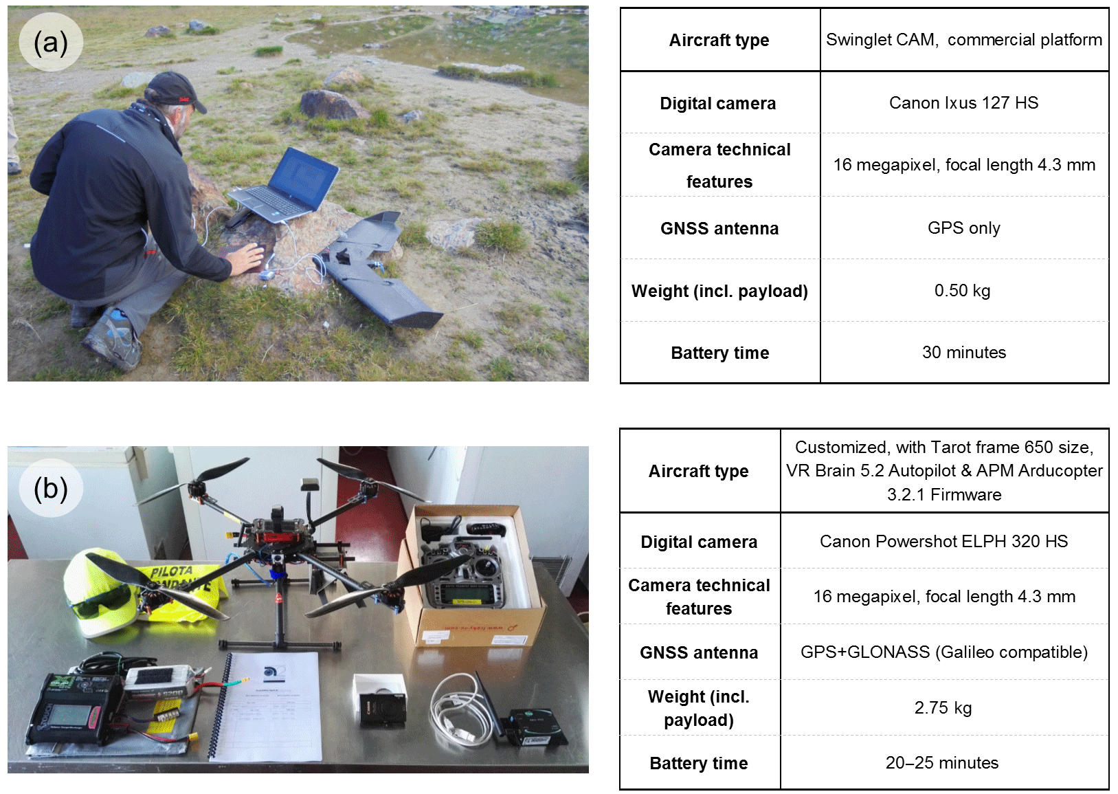
Figure 3 The UAVs used in surveys of the Forni Glacier and their characteristics. (a) The SwingletCam fixed-wing aircraft employed in 2014, at its take-off site by Lake Rosole; (b) the customized quadcopter used in 2016 in the lab.

Several flights were conducted to cover a small section of the proglacial plain and different surface types on the glacier surface, including the terminus, a collapsed area on the central tongue, the eastern medial moraine and some debris-covered parts of the eastern tongue. A “zig-zag” flying scheme was followed to reduce the flight time. The UAV was flown in autopilot mode using the open-source software Mission Planner (Oborne, 2013) to ensure 70 % along-strip overlap and side lap. In total, two flights were performed during the first survey and three during the second, lasting about 20 min each. The surveyed area spanned over 0.59 km².

Eight GCPs (see Fig. 1) were measured for the registration of the photogrammetric blocks and its byproducts into the mapping system. The root mean square error (RMSE) of the GCP location was 40 cm, which can be used as an indicator of the internal consistency of the photogrammetric block. The point cloud obtained from the 2016 UAV flight was interpolated to produce a DEM and orthophoto with the same cell resolution as the 2014 dataset, i.e., 60 and 15 cm, respectively. Both products were exported in the ITRS2000/UTM 32N mapping reference system.

3.2 Terrestrial photogrammetry

The terrestrial photogrammetric survey was carried out on 29 August 2016 to reconstruct the topographic surface of the glacier terminus, which presented several vertical and subvertical surfaces (see Fig. 2e) whose measurement was not possible from the UAV platform carrying a camera in nadir configuration.

Images were captured from 134 ground-based stations, most of them located in front of the glacier and some on both flanks of the valley in the downstream area. A single-lens-reflex Nikon D700 camera was used, equipped with a 50 mm lens, and a full-frame CMOS sensor (36 × 24 mm) with 4256 × 2823 pixels. In this case, since no preliminary information about approximate camera position was collected, the SfM procedure was run without any initial information.

Seven natural features visible on the glacier front were used as GCPs to be included in the bundle adjustment computation. Measurement of GCPs in the field was carried out by means of a high-precision theodolite. The measurement of points previously recorded with a GNSS geodetic receiver made it possible to register the coordinates of GCPs in the mapping reference system. The RMSE of 3-D residual vectors on GCPs was 34 cm.

3.3 Terrestrial laser scanning

On the same days as the first UAV survey of 2016, a long-range terrestrial laser scanner Riegl LMS-Z420i was used to scan the glacier terminus. One instrumental standpoint located on the hydrographic left flank of the glacier terminus (see Fig. 1) was established. The horizontal and vertical scanning resolution were set up to provide a spatial point density of approx. 5 cm on the ice surface at the terminus. Georeferencing was accomplished by placing five GCPs consisting in cylinders covered by retroreflective paper. The coordinates of GCPs were measured by using a precision theodolite following the same procedure adopted for terrestrial photogrammetry. Considering the accuracy of registration and the expected precision of laser point measurement, the global uncertainty of 3-D points was estimated on the order of ±7.5 cm.

3.4 GNSS ground control points

Prior to the 2016 surveys, eight control targets were placed both on the periglacial area and on the glacier tongue (see Fig. 1). Differential GNSS data were acquired at the target location for the georeferencing of UAV, terrestrial photogrammetry and TLS data. GCPs were used (1) to georeference UAV data directly, by identifying the targets on the images in Photoscan and (2) to register theodolite measurements for georeferencing terrestrial photogrammetry and TLS. The targets consisted in a square piece of white fabric (80 × 80 cm), with a circular marker in red paint chosen to provide contrast against the background. Except for the one GCP located at the highest site, such GCPs were positioned on large, flat boulders to provide a stable support and reduce the impact of ice ablation between flights.

GNSS data were acquired by means of a pair of Leica Geosystems 1200 geodetic receivers working in RTK (real-time kinematics) mode (see Hoffman-Wellenhof et al., 2008). One of them was set up as master on a precise point beside Branca hut, with known coordinates in the mapping reference system ITRS2000/UTM 32N. The second receiver was used as a rover, communicating via radio link with the master station. The maximum distance between master and rover was less than 1.5 km, but some points were measured in static mode with measurement time of approximately 12 min due to the local topography preventing the radio link and the lack of mobile phone services (for RTK). The theoretical uncertainty of GCPs provided by the processing code was on the order of 2–3 cm.

3.5 2007 DEM

The 2007 TerraItaly DEM was produced by the BLOM CGR company for the Lombardy region. It is the final product of an aerial survey over the entire region, conducted with a multispectral push broom Leica ADS40 sensor acquiring images from a flying height of 6300 m with an average GSD of 65 cm. The images were processed to generate a DEM with a cell resolution of 2 m × 2 m and a ±3 m uncertainty. We converted the DEM from the “Monte Mario” to the “ITRS2000” datum and the height from ellipsoidal to geodetic using the official software for datum transformation in Italy (Verto ver. 3).

Figure 4 Location of different glacier features or hazard-prone areas on the tongue of Forni Glacier were the point cloud comparison was performed. The background image is the merged point cloud generated from the 2016 UAV and terrestrial photogrammetry survey.

4 Methods

4.1 Analysis of point clouds from the 2016 campaign: UAV/terrestrial photogrammetry and TLS

The comparison between point clouds generated during the 2016 campaign had the aim of assessing their geometric quality before their application for the analysis of hazards. These evaluations were also expected to provide some guidelines for the organization of future investigations in the field at the Forni Glacier and in other Alpine sites. Specifically, we analyzed point density (points m⁻²) and completeness, i.e., % of area in the ray view angle. Point density partly depends upon the surveying technique used, since it is controlled by the distance between sensor and surface, and determines spatial resolution. In SfM photogrammetry, point density is affected by image texture, sharpness and resolution, which influence the performance of dense matching algorithms (Dall'Asta et al., 2015), while in TLS it can be set up as a data acquisition input parameter. In this study, the number of neighbors N (inside a sphere of radius R = 1 m) divided by the neighborhood surface was used to evaluate the local point density D in CloudCompare (http://www.cloudcompare.org). To understand the effect of point density dispersion (Teunissen, 2009), the inferior 12.5 percentile of the standard deviation σ of point density was also calculated. The use of these local metrics allowed us to distinguish between point densities in different areas, since this may largely change from one portion of surface to another. A further metric in this sense was point cloud completeness, referring to the presence of enough points to completely describe a portion of surface. In this study, the visual inspection of selected sample locations was used to identify occlusions and areas with lower point density.

To analyze these properties, five regions were selected (see Fig. 4), located on the glacier topographic surface and characterized by different glacier features and the presence of hazards: (1) a glacial cavity composed of subvertical and fractured surfaces over 20 m high and forming a typical semicircular shape; (2) a glacial cavity over 10 m high with the same typical semicircular shape as location 1, covered by fine- and medium-sized rock debris; (3) a normal fault over 10 m high; (4) a highly collapsed area covered by fine- and medium-sized rock debris and rock boulders; and (5) a planar surface with a normal fault covered by fine- and medium-sized rock debris and rock boulders. The analysis of local regions was preferred to the overall analysis of all the point clouds due to (1) the incomplete overlap between point clouds obtained from different methods and (2) the opportunity to investigate the performances of the techniques in diverse geomorphological situations.

Within the same sample locations, we compared the point clouds in a pairwise manner. Since no available benchmarking data set (e.g., accurate static GNSS data) was concurrently collected during the 2016 campaign, the TLS point cloud was used as a reference. When comparing both photogrammetric data sets, the one obtained from the UAV was used as reference because of the even distribution of point density within the sample locations. The presence of residual, non-homogenous georeferencing errors in the data sets required a specific fine registration of each individual sample location, which was conducted in CloudCompare using the ICP (iterative closest point) algorithm (Pomerleau et al., 2013). ICP iteratively matches a source point cloud to a reference point cloud in Euclidean space and calculates the necessary rotation and translation to align the source point cloud with the reference based on minimization of a distance metric in a point-to-point fashion. After fine registration, point clouds in corresponding sample areas were compared using the M3C2 algorithm implemented in CloudCompare (Lague et al., 2013). As discussed in Fey and Wichmann (2016), the distance between a pair of point clouds is often evaluated by comparing elevations at corresponding nodes of DEMs, after resampling of the original data. This approach works properly when both point clouds are approximately aligned along the same planar direction, but not when there are structures with different alignments as in the case of the glacier surfaces under investigation. In fact, the M3C2 algorithm does not always evaluate the distance between two point clouds along the same directional axis, but computes a set of local normals using points within a radius D depending on the local roughness, which is directly estimated from the point cloud data, and also considering the accuracy of preliminary local registration refinement using ICP. In this case, a radius D of 20 cm and a pre-registration accuracy of 5 cm were considered, the latter obtained from ICP residuals. This solution allowed us to remove registration errors from the analysis and focus on the capability of the adopted techniques to reconstruct the local geometric surface of the glacier in an accurate way.

4.2 Point cloud merging

To improve coverage of different glacier surfaces, including planar areas and normal faults, photogrammetric point clouds from the 2016 campaign (UAV and terrestrial surveys) were merged. We chose to avoid TLS and employed the two lower-cost techniques (Chandler and Buckley, 2016) to assess their potential for combined future use. Prior to point cloud merging, a preliminary co-registration was performed on the basis of the ICP algorithm in CloudCompare. Regions common to both point clouds were used to minimize the distances between them and find the best co-registration. The point cloud from UAV photogrammetry, which featured the largest extension, was used as reference during co-registration, while the other was rigidly transformed to fit with it. After many iterations, both point clouds were aligned according to the best solution found by the ICP. In order to remove redundant points and to obtain a homogenous point density, the merged point cloud (see Fig. 5) was subsampled keeping a minimum distance between adjacent points of 20 cm. The final size of this merged data set is approximately 4.4 million points. The RGB color information associated with each point in the final point cloud was derived by averaging the RGB information of original points in the subsampling volumes. While this operation resulted in losing part of the original RGB information, it helped to provide a realistic visualization of the topographic model and therefore to interpret glacier hazards.

Figure 5 Maps of point density in sample location 2.

4.3 Glacier hazard mapping

The investigation of glacier hazards was conducted using the point cloud and orthophoto from the 2014 UAV data set as well as the merged (UAV and terrestrial) point cloud and orthophoto from 2016. In this study, we focused on ring faults and normal faults, which were identified by visually inspecting their geometric properties in the point clouds and manually delineated, while color information from orthophotos was used as a cross check. On orthophotos, both types of structures generally appear as dark linear features owing to shadows projected by fault scarps. As these structures may look similar to crevasses, further information concerning their orientation and location needs to be assessed for discrimination. The orientation of fault structures is not coherent with glacier flow, with ring faults also appearing in circular patterns. Their location is limited to the glacier margins, medial moraines and terminus, whereas crevasses can appear anywhere on the glacier surface (Azzoni et al., 2017). After delineation, we also analyzed the height of vertical facies using information from the point clouds.

4.4 DEM co-registration for glacier thickness change estimation

Several studies have found that errors in individual DEMs, both in the horizontal and vertical domain, propagate when calculating their difference, leading to inaccurate estimations of thickness and volume change (Berthier et al., 2007; Nuth and Kaab, 2011). In the present study, different approaches were adopted for georeferencing all the DEMs used in the analysis of the volume change of the Forni Glacier tongue (2007, 2014, 2016). To compute the relative differences between the DEMs, a preliminary co-registration was therefore required. The method proposed by Berthier et al. (2007) for the co-registration of two DEMs was separately applied to each DEM pair (2007–2014; 2007–2016; 2014–2016). Following this method, in each pair one DEM plays as reference (“master”), while the other is used as “slave” DEM to be iteratively shifted along x and y axes by fractions of a pixel to minimize the standard deviation of elevation differences with respect to the master DEM. Only areas assumed to be stable are considered in the calculation of the co-registration shift. The ice-covered areas were excluded by overlaying the glacier outlines from D'Agata et al. (2014) for 2007 and Fugazza et al. (2015) for 2014. The oldest DEM, which is also the widest in each comparison, was always set as the master. To co-register the 2014 and 2016 DEMs with the 2007 DEM, both were resampled to 2 m spatial resolution, whereas the comparison between 2014 and 2016 was carried out at the original resolution of these data sets (60 cm).

All points resulting in elevation differences greater than 15 m were labeled as unreliable, and consequently discarded from the subsequent analysis. Such greater discrepancies may denote errors in one of the DEMs or unstable areas outside the glacier. Values exceeding this threshold, however, were only found in a marginal area with low image overlap in the comparison between the 2014 and 2016 DEMs, with a maximum elevation difference of 36 m. Once the final co-registration shifts were computed (see Table 1), the coefficients were subtracted from the top left coordinates of the slave DEM; the residual mean elevation difference was also subtracted from the slave DEM to bring the mean to zero. After DEM co-registration, the resulting shifts reported in Table 1 were applied to each slave DEM, including the entire glacier area. Then the elevations of the slave DEM were subtracted from the corresponding elevations of the master DEM to obtain the so-called DEM of differences (DoD). Over a common glacier area (Fig. 1), we estimated the volume change and its uncertainty, which can be expressed as the combination of (1) uncertainty due to errors in elevation and (2) the truncation error caused by the use of a discrete sum (sum of DoD at each pixel multiplied by pixel area) in place of the integral in volume calculation (Jokinen and Geist, 2010). We calculated the former following the approach of Rolstad et al. (2009), taking into account spatial autocorrelation of elevation change over stable areas, considering a correlation length of 50 m; for the latter, we used the method described by Jokinen and Geist (2010).

5 Results

5.1 Point cloud analysis

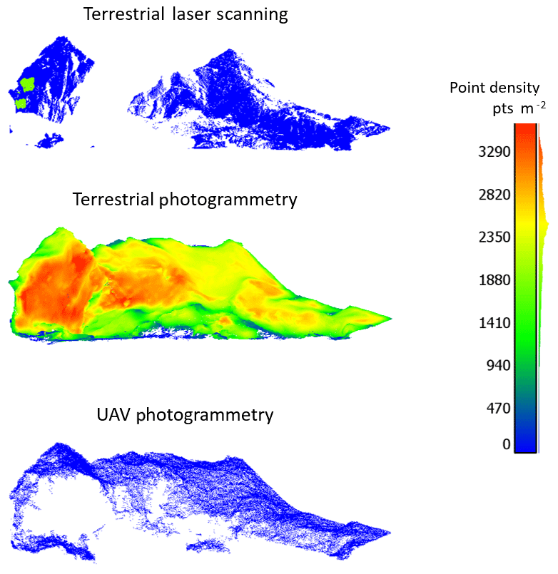
The analysis of point density shows significant differences between the three techniques for point cloud generation (see Table 2). Values range from 103 to 2297 points m⁻² depending on the surveying method, but the density was generally sufficient for the reconstruction of the different surfaces shown in Fig. 4, except for location 5. Terrestrial photogrammetry featured the highest point density, while UAV photogrammetry had the lowest. In relation to UAV photogrammetry, similar point densities were found in all sample locations, especially for the standard deviations that were always in the 22–29 point m⁻² range. Mean values were 103–109 points m⁻² in locations 2–4, while they were higher in location 5 (141 points m⁻²). Due to the nadir acquisition points, the 3-D modeling of vertical/subvertical cliffs in location 1 was not possible. In relation to TLS, a mean value of point density ranging from 141 to 391 points m² was found, with the only exception of location 5, where no sufficient data were recorded due to the position of this region with respect to the instrumental standpoint. Standard deviations ranged between 69 and 217 points m², moderately correlated with respective mean values. The analysis of the completeness of surface reconstruction also revealed some issues related to the adopted techniques (see Fig. 5). Specifically, TLS suffered from severe occlusions, which prevented acquisition of data in the central part of the sample area, while UAV photogrammetry was able to reconstruct the upper portion of the sample area but not the vertical cliff. Only terrestrial photogrammetry acquired a large number of points in all areas.

Table 1 Statistics of the elevation differences between DEM pairs before and after the application of co-registration shifts. DEM 2007 is from aerial multispectral survey; DEM 2014 and DEM 2016 are from UAV photogrammetry.

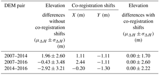
Table 2 Area and number of points in each sample window on the Forni Glacier terminus, mean and standard deviation of local point density and number of points above the lower 12.5 % percentile in each window. k stands for thousands of points. UAV refers to UAV photogrammetry, TP to terrestrial photogrammetry and TLS to terrestrial laser scanning.

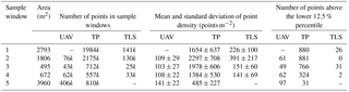
Table 3 Statistics on distances between point clouds computed on the basis of the M3C2 algorithm, showing mean, standard deviation and root mean square error (RMSE) of each point cloud pair. UAV refers to UAV photogrammetry, TP to terrestrial photogrammetry and TLS to terrestrial laser scanning. Ref. stands for reference and “–” means no comparison was performed.

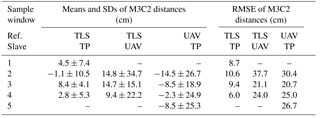
In terms of point cloud distance (see Table 3), the comparison between TLS and terrestrial photogrammetry resulted in a high similarity between point clouds, with no great differences between different sample areas. Conversely, the comparison between TLS and UAV photogrammetry and terrestrial and UAV photogrammetry provided significantly worse results, which may be summarized by the RMSEs in the ranges of 21.1–37.7 and 20.7–30.4 cm, respectively. The greater deviations were in both cases obtained in the analysis of location 2, which mostly represents a vertical surface, while the best agreement was found within location 3, which is less inclined. As the UAV flight was georeferenced on a set of GCPs with an RMSE of 40.5 cm, the ICP co-registration may have not totally compensated the existing bias.

In terms of spatial coverage, considering the entire surface examined using each technique outside the sample locations, the UAV survey extended over the widest area (0.59 km²), including part of the proglacial plain, the entire terminus and the glacier tongue up to the collapsed area on the central part, but with data gaps on the vertical and subvertical walls (see Fig. 6a). The point cloud obtained from terrestrial photogrammetry covered approximately a third of the area surveyed with the UAV (see Fig. 6b), including the full glacier terminus at very high spatial resolution, with the exception of a few obstructed parts, while the TLS point cloud covered the terminus, although with some holes due to the obstructions.

5.2 Glacier-related hazards and risks

The tongue of Forni Glacier hosts several hazardous structures, including crevasses, normal faults and ring faults. In this study, we focused on the latter two due to their relationship with glacier downwasting. While most collapsed areas on Forni Glacier are normal faults, two large ring fault systems can be identified: the first, located in the eastern section (see Figs. 2d and 7), covered an area of 25.6 × 10³ m² and showed surface dips of up to 5 m in 2014. This area was not surveyed in 2016, since field observation did not show evidence of further significant subsidence. Conversely, the ring fault that only emerged as a few semicircular fractures in 2014 grew until cavity collapse, with a vertical displacement up to 20 m. Additional fractures, extending southeastward (see Figs. 2c and 7), formed between 2014 and 2016, suggesting that the extent of the collapse might widen in the near future. In 2014, further ring faults were also identified at the eastern glacier margin, and the one that was surveyed in 2016 showed evidence of increasing subsidence (+2 m) and the formation of additional subparallel fractures.

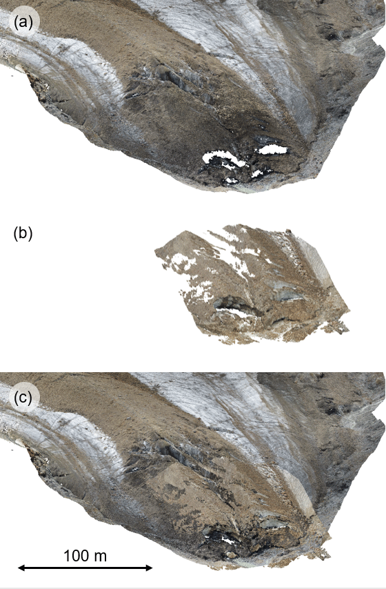
Figure 6 Spatial coverage of UAV and terrestrial photogrammetry point clouds and merged point cloud from the two techniques. (a) UAV photogrammetry point cloud; (b) terrestrial photogrammetry point cloud; (c) merged point cloud.

Normal faults are mostly found on the eastern medial moraine and at the terminus. Between 2014 and 2016, the first (see Fig. 2a) developed rapidly in the vertical domain reaching a height of 12 m in 2016. The latter increased in number as size, as the terminus underwent collapse, leading to the formation of three major ice cavities, up to 24 m high (see Fig. 2b and e). In 2016, ice thickness above the cavity vault was between 5 and 10 m (see Fig. 4, location 1). Several fractures identified as normal faults also appear in conjunction with the large ring fault located in the central section of the glacier, extending the fracture system to the western glacier margin.

The presence of cavities at the terminus, which is easily reached in a 45 min walk from Branca hut, is particularly hazardous for tourists, because of (1) the danger of cavity collapse and (2) the potential fall of large boulders or blocks of ice from the ice cliffs. Other fracture systems located higher up glacier are presumably reached by more experienced hikers. Most ring faults, however, show evidence of vertical and horizontal expansion, and further cavity collapse would imply a severe risk of injury and death if hikers were involved.

The location of structures in 2016 suggests that the glacier terminus will recede through ice cliff backwasting and cavity collapse along the fault system on the eastern medial moraine and along the ring faults at the eastern and western margins, potentially compromising access to the glacier. Since this system of fractures has been developing very rapidly, and new collapses have already been documented in September 2017, the risk for people walking on the glacier tongue during summer should be carefully evaluated. Although surface features may be visually detected, the availability of detailed 3-D models that depict the entire outer surface of the glacier is a great advantage because it allows quickly capturing the glacier topography remotely, helping predict the possible development of new collapses and understand their mechanisms of formation.

Table 4 Average ice thickness change, thinning rates and volume loss from DEM differencing over a common reference area of 0.32 km² for all DEM pairs. Uncertainty of thickness change expressed as 1 standard deviation of residual elevation differences over stable areas after DEM co-registration.

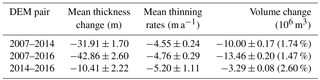
Figure 7 Location of collapse structures, i.e., normal faults and ring faults and trails crossing the Forni Glacier. (a) Collapse structures in 2014, with 2014 UAV orthophoto as base map. The red box marks the area surveyed in 2016. (b) Collapse structures in 2016, with 2016 UAV orthophoto as base map. Trails from Kompass online cartography at https://www.kompass-1039 italia.it/info/mappa-online/.

Figure 8 Ice thickness change rates from DEM differencing over (a) 2007–2014, (b) 2007–2016 and (c) 2014–2016. Glacier outlines from 2014 and 2016 are limited to the area surveyed during the UAV campaigns. Base map from hill shading of 2007 DEM.

5.3 Glacier thickness change

The Forni Glacier tongue was affected by substantial thinning throughout the observation period. Between 2007 and 2014, the greatest thinning occurred in the eastern section of the glacier tongue, with changes persistently lower than −30 m (more than 4 m a⁻¹ thinning), whereas the upper part of the central tongue only thinned by 10–18 m (between approximately 1 and 2.5 m a⁻¹). The greatest ice loss occurred in correspondence with the normal faults localized in small areas at the eastern glacier margin (see Fig. 8a), with local changes generally lower than −50 m (more than 7 m a⁻¹ thinning) and a minimum of −66.80 m, owing to the formation of a lake. Conversely, between 2014 and 2016 the central and eastern parts of the tongue had similar thinning patterns, with average changes of −10 m (5 m a⁻¹). The greatest losses are mainly found in correspondence with normal faults, with a maximum change of −38.71 m at the terminus and local thinning greater than 25 m on the lower medial moraine. The ring fault at the left margin of the central section of the tongue also shows thinning of 20 to 26 m (10–13 m a⁻¹). In the absence of faults, little thinning occurred instead on the upper part of the medial moraine, where a thick debris cover shielded ice from ablation, with changes of −2 to −5 m (1 to 2.5 m a⁻¹; see Fig. 8c). Considering a common reference area (see Fig. 1, Table 4), an acceleration of glacier thinning seems to have occurred over recent years over the lower glacier tongue, from −4.55 ± 0.24 m a⁻¹ in 2007–2014 to −5.20 ± 1.11 m a⁻¹ in 2014–2016, also confirmed by the value of −4.76 ± 0.29 m a⁻¹ obtained from the comparison between 2007 and 2016. Looking at the first two DoDs, the trend seems to be caused by the increase in collapsing areas (Fig. 8a and b). In all DoDs, the uncertainty in ice thickness change affects less than 3 % of the respective volume change (see Table 4).

6 Discussion: comparison of techniques for point cloud generation

The choice of a technique to monitor glacier hazards and the glacier thickness changes depends on several factors, including the size of the area, the desired spatial resolution and accuracy, logistics and cost. In this study, we focused on spatial metrics, i.e., point density, completeness and distance between point clouds, to evaluate the performance of UAV, close-range photogrammetry and TLS in a variety of conditions.

6.1 Point density and completeness

Considering point density, terrestrial photogrammetry resulted in a denser data set than the other techniques. This is mostly motivated by the possibility of acquiring data from several stations using this methodology, depending only on the terrain accessibility, reducing the effect of occlusions with a consequently more complete 3-D modeling. However, the mean point density achieved when using terrestrial photogrammetry is highly variable, both between different sample locations and within each location as shown by the standard deviations of D. Point densities related to UAV photogrammetry and TLS are more regular and constant. In the case of UAV photogrammetry, the homogeneity of point density might be due to the regular structure of the airborne photogrammetric block. In the case of TLS, the regularity is motivated by the constant angular resolution adopted during scanning. Since any technique may perform better when the surface to survey is approximately orthogonal to the sensor's point of view, terrestrial photogrammetry is more efficient for reconstructing vertical and subvertical cliffs (sample areas 1 and 2) and high-sloped surfaces (sample areas 3 and 4). In contrast, airborne UAV photogrammetry provided the best results in location 5 which is less inclined and consequently could be well depicted in vertical photos. In general, point clouds from terrestrial photogrammetry provide a better description of the vertical and subvertical parts (see, e.g., Winkler et al., 2012), while point clouds obtained from UAV photogrammetry are more suitable to describe the horizontal or subhorizontal surfaces on the glacier tongue and periglacial area (Seier et al., 2017), unless the camera is tilted to an off-nadir viewpoint (Dewez et al., 2016; Aicardi et al., 2016). Results obtained from photogrammetry based on terrestrial and UAV platforms can thus be considered quite complementary and they support the concept of merging the point clouds from these two techniques, as seen in Fig. 6c. In agreement with other studies of vertical rock slopes (e.g., Abellán et al., 2014), we found that the TLS point cloud was affected by occlusions (see, e.g., location 2 in Figs. 4 and 5), which can only be compensated by increasing the number of stations. Data acquisition with this platform was in general difficult in regions subparallel to the laser beams and in the presence of wet surfaces.

6.2 Point cloud and DEM uncertainty

In this study, the distance between the UAV and TLS point clouds (21.1–37.7 cm RMSE), assumed as a measure of the uncertainty of the 2016 UAV data set, was slightly higher than previously reported in high mountain glacial environments (e.g., Immerzeel et al., 2014; Gindraux et al., 2017; Seier et al., 2017), although in these studies the comparison was between DEMs and GNSS control points. Contributing factors might include the suboptimal distribution and density of GCPs (Gindraux et al., 2017), the delay between the UAV surveys as well as between the UAV and TLS, and the lack of coincidence between GCP placement and the UAV flights. This means the UAV photogrammetric reconstruction was affected by ice ablation and glacier flow, which on Forni Glacier range between 3 and 5 cm day⁻¹ (Senese et al., 2012) and between 1 and 4 cm day⁻¹, respectively (Urbini et al., 2017). We thus expect a combined 3-day uncertainty on the 2016 UAV data set between 10 and 20 cm and lower on GCPs, considering reduced ablation due to their placement on boulders. A further contribution to the GCP error budget might stem from the intrinsic precision of GNSS and theodolite measurements and image resolution. The comparison between close-range photogrammetry and TLS was less affected by glacier change because data were collected 1 day apart and the RMSE of 6–10.6 cm is in line with previous findings by Kaufmann and Landstaedter (2008). To reduce the uncertainty of UAV photogrammetric blocks, a better distribution of GCPs or switching to an RTK system should be considered, while close-range photogrammetry could benefit from measuring a part of the photo-stations as proposed in Forlani et al. (2014) instead of placing GCPs on the glacier surface.

The uncertainty in UAV photogrammetric reconstruction also factored in the standard deviation still present after the co-registration between DEMs in areas outside the glacier (2.22 m between 2014 and 2016). Another important factor here is the morphology of the co-registration area, i.e., the outwash plain, still subject to changes due to the inflow of glacier meltwater and sediment reworking. UAV photogrammetric products permitted us to investigate ice volume changes over 2 years with an uncertainty of 2.60 %, while the integration with close-range photogrammetry was required to investigate hazards related to the collapse of the glacier terminus.

6.3 Logistics and costs

In our surveys, it became evident that the main disadvantage of TLS compared to photogrammetry is the complexity of instrument transport and setup. In terms of logistics and workload, up to five people were involved in the transportation of the TLS instruments (laser scanner, theodolite, at least two topographic tripods and poles, electric generator and ancillary accessories) while two people were required for UAV and close-range photogrammetric surveys, which were also considerably faster. Meteorological conditions and the limited access to unstable areas close to the glacier terminus also prevented the acquisition of TLS data from other viewpoints as done with photogrammetry. Concerning UAV surveys, we conducted them under different meteorological scenarios and obtained adequate results in early-morning operations with 0∕8 cloud cover and midday flights with 8/8 cloud cover. Both scenarios can provide diffuse light conditions allowing collection of pictures suitable for photogrammetric processing, but camera settings need to be carefully adjusted beforehand (O'Connor et al., 2017). If early-morning flights are not feasible in the study area for logistical reasons or when surveying glaciers with eastern exposures, the latter scenario should be considered.

In terms of costs, UAV and terrestrial photogrammetric surveys are also advantageous, since TLS instruments are much more expensive at EUR 70 000–100 000 compared to UAVs (EUR 3500 for our platform) and DSLR (digital single-lens reflex) cameras used in photogrammetry, in the EUR 500–3500 range.

6.4 Additional remarks

In summary, although TLS point clouds are regarded as the most accurate (Naumann et al., 2013), they suffer from inhomogeneous point density and cumbersome logistics, and their potential in glacial environments is limited, unless a maximum uncertainty of 5–10 cm can be tolerated. Laser scanners are also employed on aerial platforms, including UAVs, where they can reconstruct terrain morphology with only slightly higher uncertainty than the terrestrial counterparts with a much greater coverage (Rayburg et al., 2009), but the high operational cost has limited the diffusion of this technique. Lastly, photogrammetry from higher-altitude aerial platforms (mostly planes, but also helicopters and satellites) can similarly achieve low uncertainty (3 m; Andreassen et al., 2002) and extensive coverage at the price of a lower spatial resolution compared to UAVs (e.g., 2 m in our case), and due to its popularity in the past it is often the only means to acquire good quality archive data to investigate glacier changes over broad timescales (Andreassen et al., 2002; Moelg and Bloch, 2017).

In our pilot study, we covered part of the Forni Glacier tongue, and investigated different techniques to map/monitor hazards related to the glacier collapse. Our maps can help identify safer paths where mountaineers and skiers can visit the glacier and reach the most important summits. However, the increase in collapse structures owing to climate change requires multitemporal monitoring. A comprehensive risk assessment should also cover the entire glacier, to investigate the probability of serac detachment and provide an estimate of the glacier mass balance with the geodetic method. While our integrated approach using a multicopter and terrestrial photogrammetry should be preferred to TLS for the investigation of small individual ice bodies, fixed-wing UAVs, ideally equipped with an RTK system and the ability to tilt the camera off-nadir, might be the platform of choice to cover large distances (see, e.g., Ryan et al., 2017), potentially reducing the number of flights and solving issues with GCP placement. Such platforms could help collect sufficient data for hazard management strategies up to the basin scale in Stelvio National Park and other sectors of the Italian Alps, eventually replacing higher-altitude aerial surveys. Cost analyses (Matese et al., 2015) should also be performed to evaluate the benefits of improved spatial resolution and lower DEM uncertainty of UAVs compared to aerial and satellite surveys and choose the best approach for individual cases.

7 Conclusions

In our study, we compared point clouds generated from UAV photogrammetry, close-range photogrammetry and TLS to assess their quality and evaluate their potential in mapping and describing glacier hazards such as ring faults and normal faults, in a specific campaign carried out in summer 2016. In addition, we employed orthophotos and point clouds from a UAV survey conducted in 2014 to analyze the evolution of glacier hazards, as well as a DEM from an aerial photogrammetric survey conducted in 2007, to investigate glacier thickness changes between 2007 and 2016. The main findings of our study are as follows:

• UAVs and terrestrial photogrammetric surveys provide reliable performances in glacial environments and outperform TLS in terms of logistics and costs.

• UAV and terrestrial photogrammetric blocks can be easily integrated providing more information than individual techniques to help identify glacier hazards.

• UAV-based DEMs can be employed to estimate thickness and volume changes but improvements are necessary in terms of area covered and to reduce uncertainty.

• The Forni Glacier is rapidly collapsing with an increase in ring fault sizes, providing evidence of climate change in the region.

• The glacier thinning rate increased due to collapses to 5.20 ± 1.11 m a⁻¹ between 2014 and 2016.

The maps produced from the combined analysis of UAV and terrestrial photogrammetric point clouds and orthophotos can be made available through GIS web portals of the Stelvio National Park or the Lombardy region (http://www.geoportale.regione.lombardia.it/). A permanent monitoring programme should be set up to help manage risk in the area, issuing warnings and assisting mountain guides in changing hiking and ski routes as needed. The analysis of glacier thickness changes suggests a feedback mechanism which should be further analyzed, with higher thinning rates leading to increased occurrence of collapses. Glacier downwasting is also of relevance for risk management in the protected area, providing valuable data to assess the increased chance of rockfalls and to improve forecasts of glacier meltwater production.

While our test was conducted on one of the largest glaciers in the Italian Alps, the integrated photogrammetric approach is easily transferable to similarly sized and much smaller glaciers, where it would be able to provide a comprehensive assessment of hazards and thickness changes and become useful in decision support systems for natural hazard management. In larger regions, UAVs hold the potential to become the platform of choice, but their performances and cost-effectiveness compared to aerial and satellite surveys must be further evaluated.