Probabilistic hazard analysis of the gas emission of Mefite d'Ansanto, southern Italy

The emission of gas species dangerous to human health and life is a widespread source of hazard in various natural contexts. These mainly include volcanic areas but also non-volcanic geological contexts. A notable example of the latter occurrence is the Mefite d'Ansanto area in the southern Apennines in Italy. Here, large emissions of carbon dioxide (CO₂) occur at rates that make this the largest non-volcanic CO₂ gas emissions area in Italy and probably on Earth. Given the topography of the area, in certain meteorological conditions a cold-gas stream forms in the valleys surrounding the emission zone, which has proved to be potentially lethal to humans and animals in the past. In this study, we present a gas hazard modelling study that considers the main species, CO₂, and the potential effect of another notable species, hydrogen sulfide (H₂S). For these purposes, we used VolcanIc Gas dIspersion modeLling v1.3.7 (VIGIL), a tool that manages the workflow of gas dispersion simulations in both the dense- and dilute-gas regimes and is specifically optimised for probabilistic hazard applications. In its latest version, VIGIL can automatically detect the most appropriate regime to simulate based on the gas emission properties and meteorological conditions at the source. Results are discussed and presented in the form of maps of CO₂ and H₂S concentration and persistence at various exceedance probabilities, which consider the gas emission rates and their possible ranges of variation defined in previous studies. The effect of seasonal variations is also presented and discussed.

1 Introduction

Carbon dioxide (CO₂), which is naturally released into the atmosphere, is a gas that can cause harm to humans and animals above certain concentration thresholds and exposure times (e.g. the National Institute for Occupational Safety and Health (NIOSH), 1976; Granieri et al., 2013; Folch et al., 2017; Settimo et al., 2022, and references therein). In nature, CO₂ can be emitted into the atmosphere by various processes, from slow, steady emissions, diffuse soil degassing, or volcanic fumaroles (e.g. Chiodini et al., 2021) to catastrophic short-lived, large-volume emissions caused by limnic eruptions during lake overturns (e.g. Folch et al., 2017). Other scenarios are possible, such as the emission from CO₂ reservoirs in certain geological contexts. This is the case at Mefite d'Ansanto, which represents the largest non-volcanic CO₂ gas emission area in Italy and probably on Earth (Chiodini et al., 2010). In this area in the southern Apennines (Italy), during periods with stable atmosphere and low winds, the gas, denser than the surrounding air, is channelised at the bottom of an east–west-trending valley, forming a lethal and invisible gas river. The frequent occurrence of the gas river is revealed by the lack of vegetation at the bottom of the valley. Here, wild and domestic animals (dogs, cats, foxes, etc.) killed by the high concentration of CO₂ are often found. Furthermore, in the past, several lethal accidents involved humans as well. Specifically, historical chronicles of the 17th–18th century describe the death of nine people (Gambino, 1991). More recently, three people died in the 1990s (Chiodini et al., 2010).

In this work we use the computational workflow VIGIL (VolcanIc Gas dIspersion modeLling, v1.3.7) (Dioguardi et al., 2022, 2023) to carry out a probabilistic hazard analysis of cold-CO₂ emissions and streams at Mefite d'Ansanto. VIGIL is a Python tool that manages the gas dispersion simulation workflow for a wide range of applications (single forecast or reanalysis simulation, multiple reanalysis simulations, probabilistic hazard assessment applications). It allows us to simulate both passive dispersion of a gas species in the atmosphere by interfacing with DISGAS v2.5.3 (Costa et al., 2009; Costa and Macedonio, 2016; Macedonio and Costa, 2023) (http://datasim.ov.ingv.it/models/disgas.html, hereafter referred to as DISGAS) and dense-gas flows on real topography by means of TWODEE-2 v2.6 (Hankin and Britter, 1999; Folch et al., 2009, 2017, 2023) (http://datasim.ov.ingv.it/models/twodee.html, hereafter referred to as TWODEE-2). In both cases, VIGIL employs DIAGNO v1.5.0, which is a mass-consistent wind model modified after DWM (Douglas et al., 1990) (http://datasim.ov.ingv.it/models/diagno.html, hereafter referred to as DIAGNO), to simulate the meteorological conditions (wind, temperature gradients) at a high resolution in the computational domain, starting from observed or modelled meteorological conditions in single locations of the domain. The need to automatically manage the simulation workflow of an atmospheric dispersion application, which is a procedure that involves different and often time-consuming steps (meteorological data retrieval and processing, high-resolution meteorological simulations, gas dispersion simulation, analysis, and post-processing), is particularly evident for probabilistic hazard assessment (PHA) applications, in which usually a large number of simulations are carried out in order to explore the uncertainty related to the input parameters (e.g. the wind field, the gas emission rate) (Magill and Blong, 2005; Martí et al., 2008; Neri et al., 2008; Marzocchi et al., 2010; Selva et al., 2010; Sandri et al., 2014; Mead et al., 2022). PHA carried out using gas dispersion models such as TWODEE-2 and DISGAS (Costa et al., 2009; Folch et al., 2009; Costa and Macedonio, 2016) is based on multiple deterministic simulations of gas concentration in the area of interest, aimed at exploring not only the natural variability in input and boundary conditions (seasonal and daily wind variability, source position, and gas flux at the emission sources) but also the impact of the uncertainty on other controlling factors such as, for example, the resolution of topographic or meteorological data (Tierz et al., 2016; Selva et al., 2018; Massaro et al., 2021).

For the Mefite d'Ansanto application, Chiodini et al. (2010) performed TWODEE-2 simulations of the CO₂ stream only under very low-wind conditions for the period when they carried out the measurement campaign, which is when the gas river forms. In this work, thanks to the novel features introduced in VIGIL v1.3.7, we were able to explore the uncertainty related to the wide range of meteorological conditions while varying the CO₂ emission rates within the range of the confidence values reported in Chiodini et al. (2010). Specifically, in the latest version, it is possible to automatically determine the most appropriate gas dispersion scenario (dense-gas flow or dilute-gas advection–diffusion) based on the gas emission properties and meteorological conditions at the source (see Sect. 3.1.2). In this way, we were able to quantify the probabilistic hazard of the CO₂ concentration in the Mefite d'Ansanto area without a priori focusing on the gas river scenario. Furthermore, knowing the chemical composition data for the Mefite gas emissions, we were also able to obtain a first insight into the hazard of hydrogen sulfide (H₂S).

In the following, we summarise the geological origin of these steady intense CO₂ emissions in the Mefite d'Ansanto area; then we briefly recall the features of VIGIL and its capabilities; and finally, we present the modelling strategies and the PHA outputs and their implications for the safety of livestock and people in the area.

2 Geological origins of the Mefite d'Ansanto gas emissions

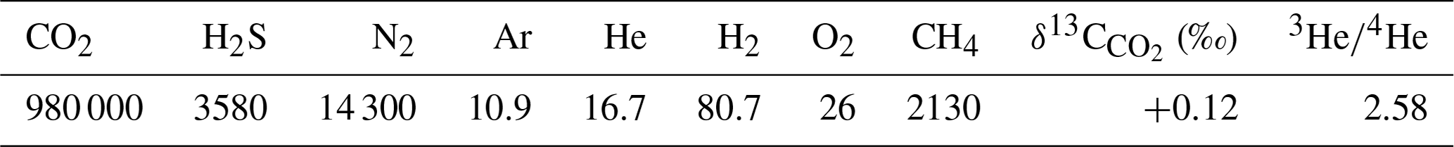
Carbon-dioxide-dominated gas emissions and groundwater rich in deeply derived CO₂ affect a large portion of the western side of the Apennine chain; the gas at the root of which is thought to be generated by the melting of carbonates of the subducting Adria plate (Chiodini et al., 2004; Frezzotti et al., 2009; Di Luccio et al., 2022). Mefite d'Ansanto is the biggest of the numerous cold-gas emission areas (>150 km²) located in this sector of the Italian peninsula (http://www.magadb.net; Chiodini et al., 2010, and references therein). The isotopic signatures of He and CO₂ (${}^{\mathrm{3}}\mathrm{He}/{}^{\mathrm{4}}\mathrm{He}$ ratio expressed as $R/\mathit{\text{Ra}}$ of 2.58 and ${\mathit{\delta }}_{\mathrm{13}}{\mathrm{C}}_{{\mathrm{CO}}_{\mathrm{2}}}=+\mathrm{0.12}\mathrm{‰}$, where Ra is the helium isotopic ratio in the atmosphere; Table 1) are very similar to those of the fumaroles of the Vesuvius and Campi Flegrei volcanoes (${\mathit{\delta }}_{\mathrm{13}}{\mathrm{C}}_{{\mathrm{CO}}_{\mathrm{2}}}$ from −2 ‰ to 0.5 ‰ and $R/\mathit{\text{Ra}}$ from 2.6 to 3.4; Caliro et al., 2007), a fact that suggests the presence of magma in the axial part of the sedimentary chain (Italiano et al., 2000; Chiodini et al., 2004). Among the gas species detected in the Mefite gas, it is worth noting the non-negligible presence of hydrogen sulfide (H₂S), which may be harmful or even lethal to humans at relatively low concentrations (NIOSH, 1976, 2019, 2020; OSHA, 2023) and hence can further increase the gas hazard in the area.

Table 1 Chemical and isotopic composition of Mefite gas (concentrations in µmol mol⁻¹; Rogie et al., 2000).

In its ascent towards the surface, the gas accumulates in a buried permeable structure made of limestone covered by an impermeable formation. In that zone, it forms a gas pocket at a depth of about 1 km (Fig. 1). This trap, reached by the Monte Forcuso deep well at 1100–1600 m in depth, contains a separated gas phase rich in CO₂ and feeds the Mefite gas emission at the surface (Chiodini et al., 2010, and references therein). The conceptual scheme of Fig. 1 was recently confirmed by seismic surveys (La Rocca et al., 2023).

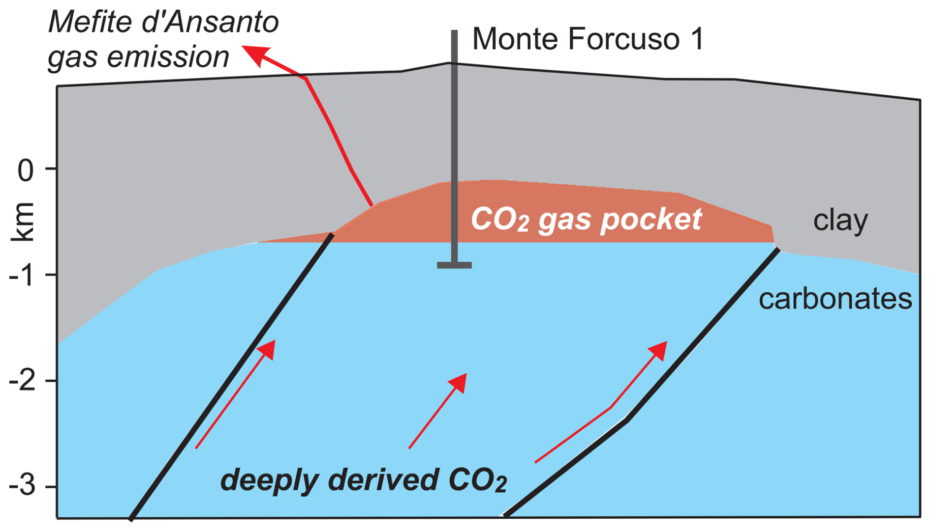
Figure 1 Section of the system feeding Mefite gas emission (redrawn with permission from Chiodini et al., 2010. Copyright 2010 by the American Geophysical Union. Geological section from Mostardini and Merlini, 1986).

3 Probabilistic hazard modelling at Mefite d'Ansanto using VIGIL

The atmospheric dispersion of a gas emitted by a natural source into the atmosphere is initially controlled by the starting density contrast between the gas and the environment (atmospheric air) and turbulent entrainment of atmospheric air driven by lateral eddies that increase the mixing with air around the edges of the plume, thereby decreasing its bulk density (Hankin and Britter, 1999; Costa et al., 2009; Folch et al., 2009; Costa and Macedonio, 2016). The flow Richardson number at the source Ri is a parameter that takes the following factors into account:

$$\begin{array}{}\text{(1)}& \mathit{\text{Ri}}={\displaystyle \frac{\mathrm{1}}{v^{\mathrm{2}}}}{\left({\displaystyle \frac{g^{\prime }q}{r}}\right)}^{\frac{\mathrm{2}}{\mathrm{3}}},\end{array}$$

where g^′ is the reduced gravity,

$$\begin{array}{}\text{(2)}& g^{\prime }=g{\displaystyle \frac{{\mathit{\rho }}_{\mathrm{g}}-{\mathit{\rho }}_{\mathrm{e}}}{{\mathit{\rho }}_{\mathrm{e}}}},\end{array}$$

which quantifies the starting buoyancy of the gas phase with starting density ρ_g relative to the environment with density ρ_e. q is the source volumetric flow rate; r is the gas plume radius at the source, which quantifies its extension; and v is the wind speed. Based on the values of Ri, two regimes are possible (Cortis and Oldenburg, 2009; Costa et al., 2013):

• If Ri<0.25, the gas transport is passive and dominated by the wind advection and diffusion (passive dispersion).

• If Ri>1, the gas transport is dominated by the density contrast between the gas and the surrounding environment; in this case, the gas flows over the topography until the density contrast persists.

Although the subsequent atmospheric gas dispersion can be theoretically simulated by solving 3D equations for the conservation of mass, momentum, and energy for each gas species, several scenario-specific simplifications are assumed in practice to reduce the computational time (i.e. a single species of gas, incompressible fluid; Costa and Macedonio, 2016), eventually approaching the two end-member scenarios represented by the DISGAS and TWODEE-2 models. In both cases, the momentum coupling with the atmospheric air, which is one-way (i.e. the atmospheric wind field influences the gas cloud or stream and not vice versa), is taken into account by considering the wind field in the computation domain (simulated with DIAGNO through VIGIL), which is the main factor controlling the light-gas dispersion and one of the controlling factors (together with density contrast) in the heavy-gas case.

DISGAS is an Eulerian model able to simulate the passive dispersal of gases in the atmosphere over complex topographic domains. It assumes that the process is governed by the wind and atmospheric turbulence and solves for the advection–diffusion equation. DISGAS allows us to specify the diffusion coefficients in 3D or using models, specifically

• the “similarity” option for the vertical-diffusion coefficient, following the Monin–Obukhov similarity theory (e.g. Monin and Yaglom, 1979; Byun, 1990) or

• the “Smagorinsky” option for the horizontal-diffusion coefficients (Smagorinsky, 1963; Pielke et al., 1992; Byun and Schere, 2006).

It is optionally coupled with the meteorological processor DIAGNO, which provides a mass-consistent gridded wind field from meteorological data (“observations”) in the computational domain. DISGAS supports uniform meteorological conditions as well, by extrapolating time series of data from a single location in a domain (e.g. a weather station). More details on DISGAS can be found in Costa and Macedonio (2016). As we have already mentioned, in this work in order to capture the topographic effects and the local variability, we model the wind field using DIAGNO (Douglas et al., 1990) initialised from the ERA5 reanalysis dataset, while the meteorological variables are calculated internally by DISGAS, as explained in Costa and Macedonio (2016), using the wind provided by DIAGNO and the ERA5 2 m surface temperatures.

On the other hand, TWODEE-2 code solves a time-dependent model for the flow of a heavy gas based on the shallow-layer approach. It is built on the depth-averaged equations for a gas cloud resulting from mixing a gas of density ρ_g with an environment fluid (air) of density ρ_e (ρ_g>ρ_e). TWODEE-2 is derived from the optimisation and generalisation of a previous Fortran 77 version of the model developed by Hankin and Britter (1999). Under the assumption that $h/L\ll \mathrm{1}$ (h being the gas cloud depth and L a characteristic length), the 2D shallow-layer approach allows a compromise between more realistic but computationally demanding 3D computational fluid dynamics (CFD) models and simpler 1D integral models. Such an approach is able to describe the cloud in terms of four variables: cloud depth, two depth-averaged horizontal velocities, and depth-averaged cloud density as functions of time and position. A full description of the physical model can be found in Folch et al. (2017, 2009). Similarly to DISGAS, TWODEE-2 supports both the uniform wind and DIAGNO options (using a shallow-layer approach, the field at only a single reference height is needed).

3.1 The gas dispersion simulation workflow with VIGIL

VIGIL (Dioguardi et al., 2022) is Python code designed to manage the simulation workflow required to carry out numerical simulations of atmospheric gas dispersion, i.e.

1. retrieving and processing the meteorological data to produce the high-resolution wind field required to simulate atmospheric gas dispersion in the computational domain, taking the topography into account via a digital elevation model (DEM);

2. running the simulation with the gas dispersion model; and

3. processing the results to produce new outputs (e.g. probabilistic outputs) and optional plots of gas concentration.

3.1.1 Step 1: meteorology

The meteorological data represent the first and most important source of uncertainty variability that VIGIL explores in its current version when PHA is conducted; this implies that if N realisations of the meteorological conditions are taken into account, VIGIL will run N dispersion simulations. Other sources of uncertainty (e.g. emission rates and gas emission source locations) can also be taken into account on top of the meteorological data variation; i.e. it is possible to apply different gas emission rates to different dispersion simulations, but these will not increase the number of the simulations N, as they are statistically sampled within the N realisations.

The source of the meteorological data depends on the chosen simulation mode (forecast or reanalysis).

• Forecast mode. NCEP (National Centers for Environmental Prediction) Global Forecast System (GFS) Numerical Weather Prediction (NWP) dataset.

• Reanalysis mode. Copernicus Climate Change Service (C3S), 2023 ERA5 NWP dataset. The user can also provide data manually, for example, using data from weather stations installed in the computational domain.

GFS and ERA5 are global models with meteorological data saved on a discrete grid, with a typical horizontal spacing of approximately 30 km. The typical domain used in the gas dispersion applications under analysis in this work and managed by VIGIL is only a few kilometres on each side, which means that the NWP data need to be interpolated into the computational domain. Furthermore, these simulations are generally carried out at a very high spatial resolution (down to few metres) in order to capture the gas clouds emitted from point sources (e.g. fumaroles) and the topographic controls on gas clouds and cold-gas streams. In order to produce reliable simulations of the gas dispersion in these contexts, simple interpolation into the domain (with the assumption that the meteorological conditions are uniform and equal to the interpolated values throughout the domain) is not sufficient, and a high-resolution weather prediction model is used to obtain a realistic wind field at the required spatial resolution, starting from the interpolated data. In this step, VIGIL, starting from the NWP interpolated data at the centre of the domain, prepares the input data to run the mass-consistent wind model DIAGNO.

3.1.2 Step 2: run the models

In this step, VIGIL runs DIAGNO to obtain the meteorological conditions in the computational domain required by DISGAS and/or TWODEE-2. Subsequently, it runs DISGAS or TWODEE-2 (based on the user's choice). Starting in version 1.3.7, a new option is available that allows the automatic detection of the scenario (light gas or heavy gas) based on the calculation of Ri (Eq. 1) for each source in the domain. This is very useful in the following situations:

• PHA applications, for which several simulations with varying meteorological conditions are carried out. In this case, it is impractical to manually a priori determine the correct choice of the scenario and, hence, of the dispersion model (DISGAS or TWODEE-2) for each simulation.

• Single simulations or PHA applications in which multiple sources with different flow rates are present in the domain. A typical situation may be a domain containing both a weak source representing diffuse degassing, which becomes wind dominated at very low wind speeds, and a strong source (e.g. a fumarole), which becomes wind dominated at higher wind speeds. In some situations, each source may behave differently as far as Ri is concerned. In such a situation, VIGIL v1.3.7 allows us to split the simulation into a DISGAS and a TWODEE-2 simulation, each one with its correct gas source. It then merges the outputs of the two simulations. Furthermore, starting in version 1.3.7, VIGIL allows us to vary the source emission rate via an empirical cumulative density function (ECDF) (whose values are provided by the user in a separate input file) and a uniform or a Gaussian distribution. The latter feature is used in this work.

This new utility exploits a new feature introduced in DIAGNO v1.5.0 that allows the user to track the wind speed at specified locations. VIGIL sets the locations at the centre of the gas sources. It is important to stress that the transport regime can change as the gas flow dilutes downstream, and it can no longer be treated accurately by TWODEE-2. This change cannot be handled by the scenario-based simulation approach employed by VIGIL. Such a limitation can only be overcome using a more complex computational fluid dynamics model, which would be more demanding in terms of computational resources and, hence, impractical to use in PHA applications. However, as explained in Sect. 5, it does not result in a significant discrepancy and, from a hazard assessment point of view, may imply a slightly cautious overestimation of the hazard.

For simplicity, VIGIL v1.3.7 closes the Ri gap between 0.25 and 1 by activating TWODEE-2 when Ri>0.25. Future versions of VIGIL will introduce a more robust management of the automatic scenarios in this range by considering the results from the two end members. For this study, we verified that using DISGAS or TWODEE-2 introduces a variation in the simulated gas concentrations in the domains that is not significant compared to the maximum expected values (see Sect. 5).

3.1.3 Step 3: post-processing of the results

This step deals with the post-processing of the DISGAS and/or TWODEE-2 results. Various functionalities are available.

• Conversion of the tracked gas species into other gas species, provided that gas species properties (e.g. molar weights, molar ratios between the converted and the tracked species) are available in a separate file.

• Production of time series of gas concentration at selected locations (tracking points).

• For PHA applications, generation of ECDFs of the gas concentration and extrapolation of the gas concentration at the user's desired exceedance probability. The ECDF is calculated by merging, at each point in the domain and for each time step, the concentrations obtained in all simulations using the Python NumPy quantile function.

• For PHA applications, if gas concentration thresholds and exposure times are provided as input, the persistence probability (i.e. the probability of overcoming a certain threshold for its exposure time) is calculated.

• For PHA applications, if the tracking point functionality is activated, hazard curves (i.e. exceedance probability vs. gas concentrations) are calculated.

Graphs of all these outputs can be optionally generated.

4 Numerical simulations of gas flow at Mefite d'Ansanto and probabilistic outputs

4.1 The PHA workflow

In this section, we review the workflow followed to carry out the PHA at Mefite d'Ansanto. All the input files and VIGIL commands required to reproduce the workflow and the outputs are available in the online Zenodo repository (Dioguardi, 2023). Details on the input files and commands can be found in the VIGIL user manual and in Dioguardi et al. (2022).

We carried out a PHA at Mefite d'Ansanto by exploring the meteorological data variability as the main source of uncertainty and, for each simulation, automatically setting the gas emission rate, sampling it from a normal distribution with a mean of 23.1 kg s⁻¹ and a standard deviation of 5.8 kg s⁻¹, according to Chiodini et al. (2010). CO₂ is emitted from an area that can be roughly approximated by a square of 3500 m², which would correspond to a radius r of 33.4 m of the equivalent circle (Fig. 2). Assuming thermal equilibrium between the emitted gas and the atmosphere, at 15 °C the two species (CO₂ and air) have a density ρ of 1.87 and 1.22 kg m⁻³, respectively. The mean volumetric flow rate q of the gas based on the mean mass flow rate is therefore 12.35 m³ s⁻¹.

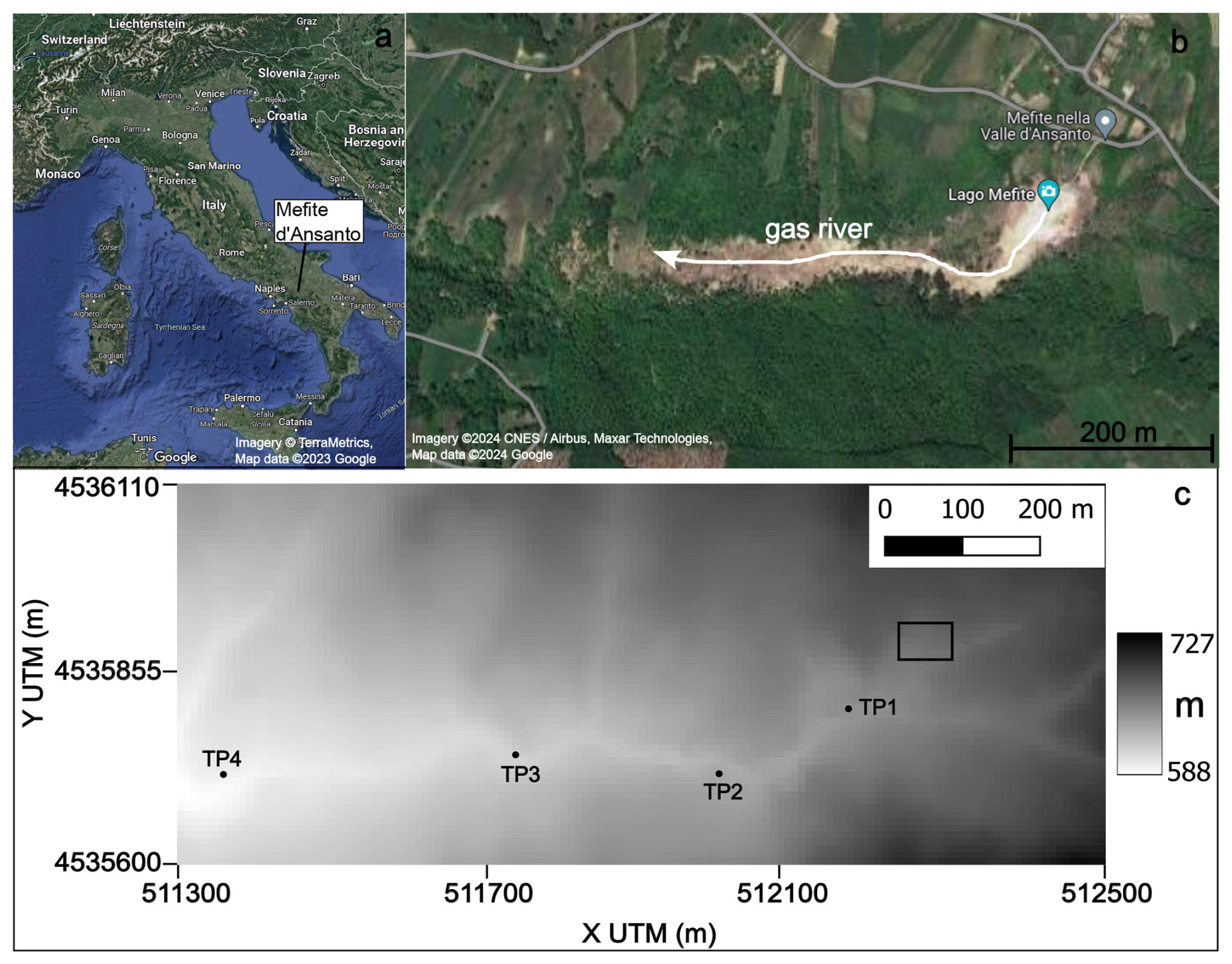
Figure 2 (a) Location of Mefite d'Ansanto in southern Italy. Imagery © TerraMetrics, map data © 2023 Google. (b) Aerial photo showing the gas emission area and the valley where the gas river forms, which is emphasised by the lack of vegetation. Imagery © 2024 CNES/Airbus, Maxar Technologies. Map data © 2024 Google. (c) Computational domain with the elevation (m a.s.l.) shown in greyscale. The CO₂ emission area approximated in the simulations is represented by the black rectangle. Black dots represent the locations of the four tracking points (TPs) where the hazard curves are extrapolated from the simulation outputs; the coordinates of the tracking points are listed in Table 4.

Meteorological conditions were retrieved from the ERA5 dataset using the weather.py script in VIGIL. Specifically, since we run 1 d long simulations with a time step of 1 h, we sampled 1000 d from the period of 1 January 1993–1 January 2023, and for each day, we downloaded pressure level (Hersbach et al., 2018a) and surface data (Hersbach et al., 2018b) for a location positioned towards the centre of the computational domain. With these data, VIGIL created the input files necessary to run DIAGNO for each day.

Subsequently, we executed run_models.py in VIGIL to first obtain the simulated meteorological wind field over 24 h with a time step of 1 h for the 1000 d in the computational domain (Fig. 2) using DIAGNO. The domain extended from 511 300 to 512 500 m E in the x direction and from 4 535 600 to 4 536 110 N in the y direction (UTM coordinates, WGS 84/UTM zone 33 N) and 500 m along the vertical and was discretised with 3 m square cells along the horizontal axes and with variable vertical spacing along the vertical direction: 1, 2, 5, 10, 20, 50, 100, 250, and 500 m. Then we selected the option to automatically detect the scenario (heavy or light gas) that was more appropriate for the simulated day based on the gas emission characteristics and the wind conditions at the source location 10 m a.g.l. (metres above ground level). We note that the emission rate varied across the 1000 d when sampling it from the normal distribution introduced above. In fact, with the gas source emission characteristics described above, the gas source satisfies the conditions of the heavy-gas regime in the case of very low to no-wind conditions. Specifically, based on Eq. (1), the maximum wind v that would satisfy the heavy-gas regime (Ri>1) is 1.25 m s⁻¹. With a wind speed of 2.49 m s⁻¹, the passive-wind-dominated conditions (Ri<0.25) would be already satisfied. As a result, 313 out of 1000 runs were simulated with TWODEE-2 (heavy-gas scenario), and the rest (687 simulations) were simulated with DISGAS.

Finally, we ran post_process.py to produce the requested outputs. We requested the following:

• ECDF 50 %, 16 %, and 5 % exceedance probability of the CO₂ concentration at 2 m a.g.l. for the time-averaged solution over the whole simulation duration (24 h). Furthermore, using the gas species conversion capability of VIGIL, we calculated the same outputs for H₂S using the chemical composition data listed in Table 1, specifically the molar ratio between H₂S and CO₂ (0.0036). However, we need to stress that such a conversion neglects possible sources or sinks of the converted species in the domain. Specifically, the reaction with OH radicals represents the main sink of H₂S in the atmosphere (e.g. Watts, 2000), together with other minor sinks that act on a local scale, e.g. during and subsequent to rainfall events (Kristmannsdottir et al., 2000; Thorsteinsson et al., 2013) or under the influence of lakes, soil, and vegetation (Bussotti et al., 1997; Cihacek and Bremner, 1990). However, these interactions typically do not play a major role, as demonstrated, for example, by Olafsdottir et al. (2014), who carried out ad hoc measurement campaigns in Iceland, showing that the depletion of H₂S from the atmosphere is insignificant compared to the emissions within a 35 km distance from the sources. Neglecting such reactions could imply an overestimation of the H₂S concentration, but we do not expect a significant effect in our restricted domain.

  It is worth noting that the current version of VIGIL does not allow the user to start the simulation from a pre-existing solution of the gas concentration field; i.e. each simulation starts with clean air (apart from background concentrations that the user may specify). This may affect the simulations' outputs in the initial time steps in scenarios such as those under analysis in this work, i.e. with steady, long-lived gas emissions. However, in a small domain such as the one under consideration, the CO₂ cloud or stream can be considered fully developed within the first hour, which is the minimum time resolution for outputs currently allowed by VIGIL due to the limitations of DIAGNO. Therefore, we can safely assume that the effect of starting from clear air is negligible in this application when we calculate the 24 h time average of the outputs.

• Persistence outputs are the probability of overcoming the concentration thresholds for their respective times, as specified in the input file specifying the gas property (gas_properties.csv). The concentration thresholds and exposure times for CO₂ used in this work are listed in Table 2 and are compiled based on NIOSH (1976, 2019, 2020), Costa et al. (2008), Granieri et al. (2013), and Settimo et al. (2022) and references therein. For 1000 and 3500 ppm, there are no time exposures indicated; therefore, we calculate the persistence for 24 h. For 5000 ppm, TWA (time-weighted average) values for CO₂ are commonly used in occupational health and safety to establish permissible exposure limits or recommended exposure limits. These limits define the maximum allowable concentration of CO₂ that a worker or individual can be exposed to over a specific time period, usually 8 h or 24 h. In this work, we take 8 h as the exposure time. For the highest concentrations taken into account (15 000, 30 000, and 100 000), the exposure times that cause harm are always in the range of 10–15 min, with the effects on humans listed in the table. In this study, for the computational limitations reported in Table 2, the minimum exposure time that we considered is 1 h. For H₂S, we used the thresholds and exposure times defined by the United States Occupational Safety and Health Administration (OSHA) (https://www.osha.gov/hydrogen-sulfide/) based on the recommendations of the National Institute for Occupational Safety and Health (NIOSH, 1976, 2019, 2020) and the base threshold defined in Olafsdottir and Gardarsson (2013). OSHA defines three limits: the recommended exposure limit (REL), the permissible exposure limit (PEL), and the immediately dangerous to life and health (IDLH) exposure limit (Table 3).

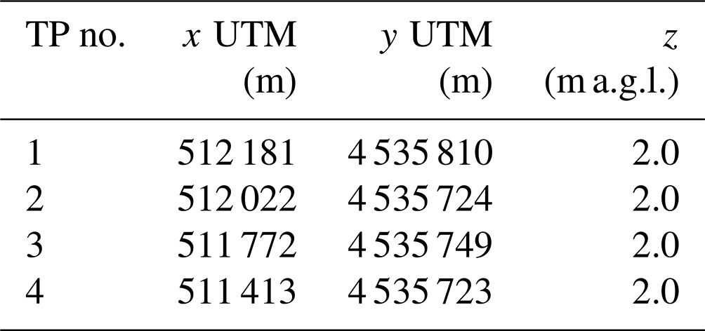
• Hazard curves, i.e. exceedance probability vs. CO₂ concentration plots, at four selected locations or tracking points (TPs; see Fig. 2) are spread along the valley. Table 4 lists the coordinates of the four tracking points.

Table 2 CO₂ concentration thresholds and exposure times that can cause harm to humans.

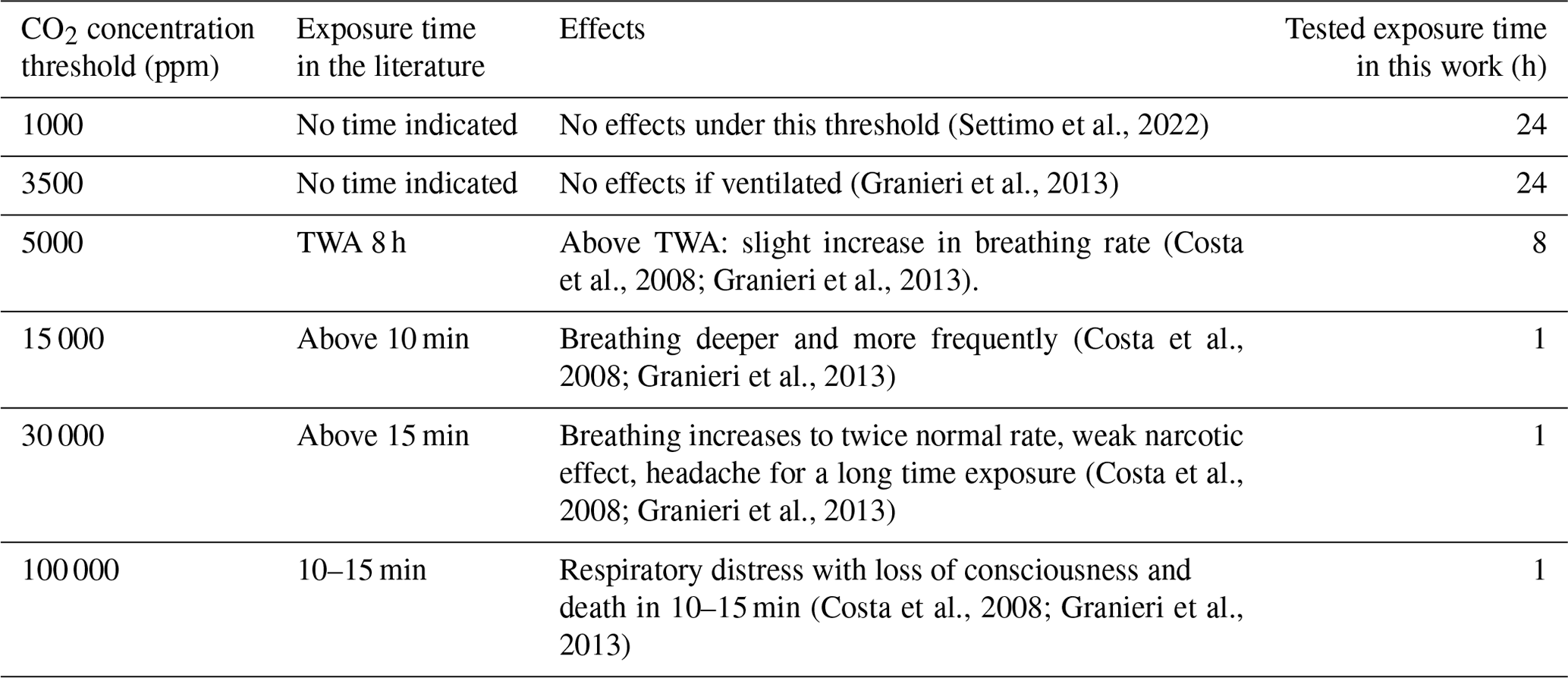
Table 3 H₂S concentration thresholds and exposure times that can cause harm to humans.

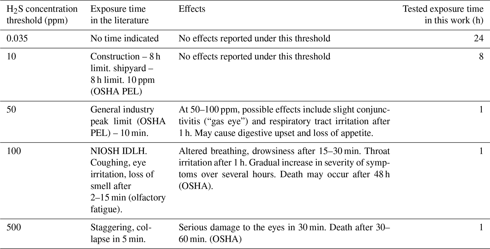
Table 4 Coordinates (UTM) and elevations (m a.g.l.) of the four tracking points used for the hazard curves.

We also carried out a seasonal analysis; i.e. we produced the aforementioned outputs for each season (winter, spring, autumn, summer) to check whether the season controls the CO₂ dispersion pattern.

4.2 Results

Figure 3 shows the concentration of CO₂ in the domain at 2 m a.g.l. at 50 %, 16 %, and 5 % exceedance probability. The concentration is obtained by interrogating the ECDF of the 24 h time-averaged solution at each point in the domain.

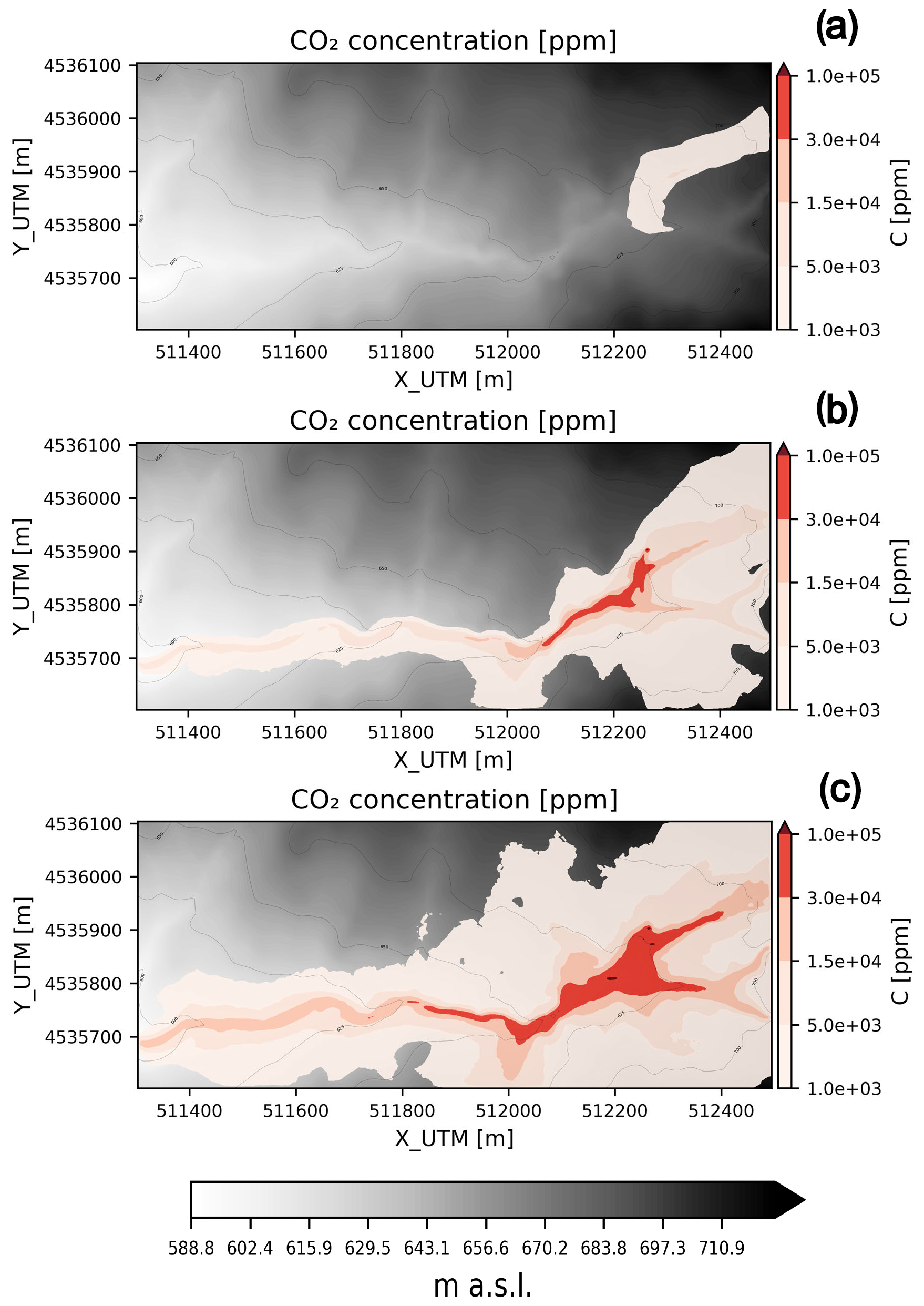
Figure 3 The 24 h time-averaged CO₂ concentration at 2 m a.g.l. at 50 % (a), 16 % (b), and 5 % (c) exceedance probabilities.

A likely situation corresponding to 50 % exceedance probability (Fig. 3a), i.e. the median of the ECDF, shows non-negligible to high (a few thousands of ppm) concentrations of CO₂ in the emission area and towards the eastern part of the domain. These areas are uphill of the emission area, which means that, on average, elevated CO₂ levels caused by the action of winds blowing from the west–southwest cannot be ruled out. At 16 % exceedance probability (Fig. 3b), which corresponds to the median + 1 standard deviation from the ECDF, the CO₂ concentration significantly increases up to dangerous levels (>15 000 ppm), and the streams along the valleys become visible. By further decreasing the exceedance probability to 5 %, which corresponds to the median + 2 standard deviations from the ECDF (Fig. 3c), the extent of the areas affected by CO₂ concentrations>15 000 ppm further increases, and eventually the gas overflows the confines of the valleys. Areas affected by CO₂ concentrations>30 000 ppm extend significantly outside the emission area at 5 % exceedance probability.

Figure 4 displays the persistence maps for the six concentration thresholds and exposure times listed in Table 2. All probabilities are calculated at 2 m a.g.l. Figure 4a shows the probability of overcoming a CO₂ concentration of 1000 ppm for at least 24 h, which is the duration of the simulation. This probability is high in the emission area but is also not negligible (5 %–10 %) along the main east–west valley and in some areas towards the northeast of the domain. This is in line with what is observed in Fig. 3a, which was interpreted as the formation of CO₂ plumes drifting northeast due to the action of winds blowing from west–southwest. Figure 4b shows the probability of overcoming a CO₂ concentration of 3500 ppm for at least 24 h. As expected, the probability is lower than the case shown in Fig. 3a but is still not negligible along the main valley and in the emission area and surroundings. Considering an exposure time of 8 h, the probability of overcoming a CO₂ concentration of 5000 ppm is high in the emission area and surroundings (up to 50 %), lower but still notable towards the east–northeast (up to 30 %), and not negligible along most of the valleys (10 %–20 %) (Fig. 4c). Focusing on high (15 000–30 000 ppm) to very high (100 000 ppm) concentrations for an exposure time of 1 h (Fig. 4d–f, respectively), the extent of the domain affected by significant probabilities is noteworthy for 15 000 and 30 000 ppm, with probabilities up to 50 %–60 % in the emission area and surroundings (particularly towards the northeast) and along the valleys (up to 20 %–30 %). Even in the most extreme case of CO₂ concentrations>100 000 ppm, there is a 30 % probability of overcoming this concentration for 1 h in the emission area and surroundings and a non-negligible (up to 10 %–20 %) one along the valleys.

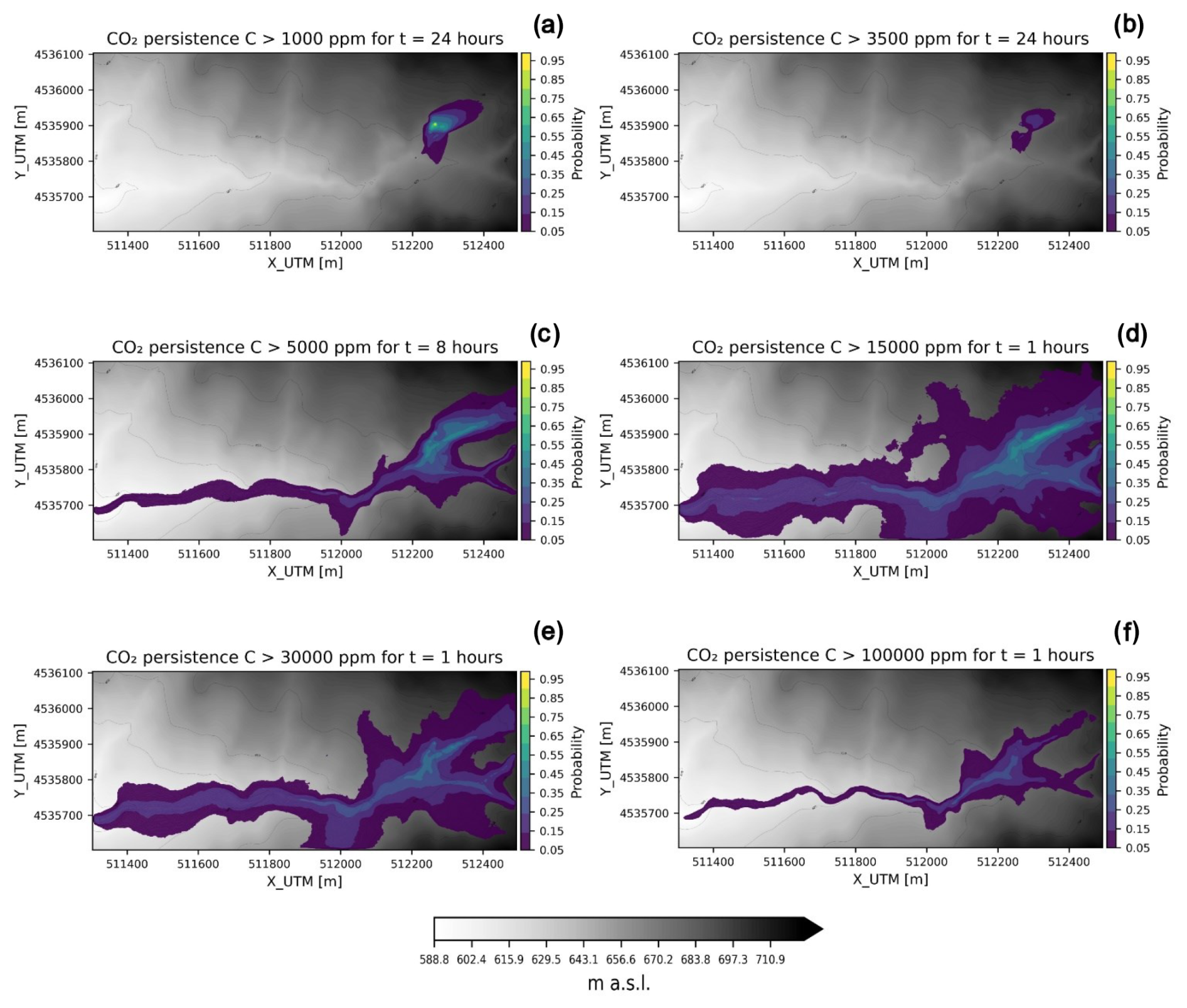
Figure 4 Persistence maps at 2 m a.g.l. (a) The concentration threshold is 1000 ppm, and the exposure time is 24 h. (b) Concentration threshold of ppm and exposure time of 24 h. (c) Concentration threshold of 5000 ppm and exposure time of 8 h. (d) Concentration threshold of 15 000 ppm and exposure time of 1 h. (e) Concentration threshold of 30 000 ppm and exposure time of 1 h. (f) Concentration threshold of 100 000 ppm and exposure time of 1 h.

The hazard curves of the 24 h averaged CO₂ concentration produced at the four locations identified by the four tracking points listed in Table 4 and shown in Fig. 2 are represented in Fig. 5. At the location TP1, which is the closest to the emission area, higher concentrations of CO₂ than the other locations are expected; i.e. for a fixed exceedance probability, the concentration is significantly higher. The maximum concentration is close to 140 000 ppm. The curves at the other locations show similar values, although they are slightly higher for TP2, which is the second closest to the emission area. Looking at Fig. 2c, TP2, TP3, and TP4 are positioned along the main east–west valley. The fact that the concentrations are almost the same, especially at TP3 and TP4, can be interpreted as the CO₂ stream maintaining its characteristics along the valley, at least in the domain analysed.

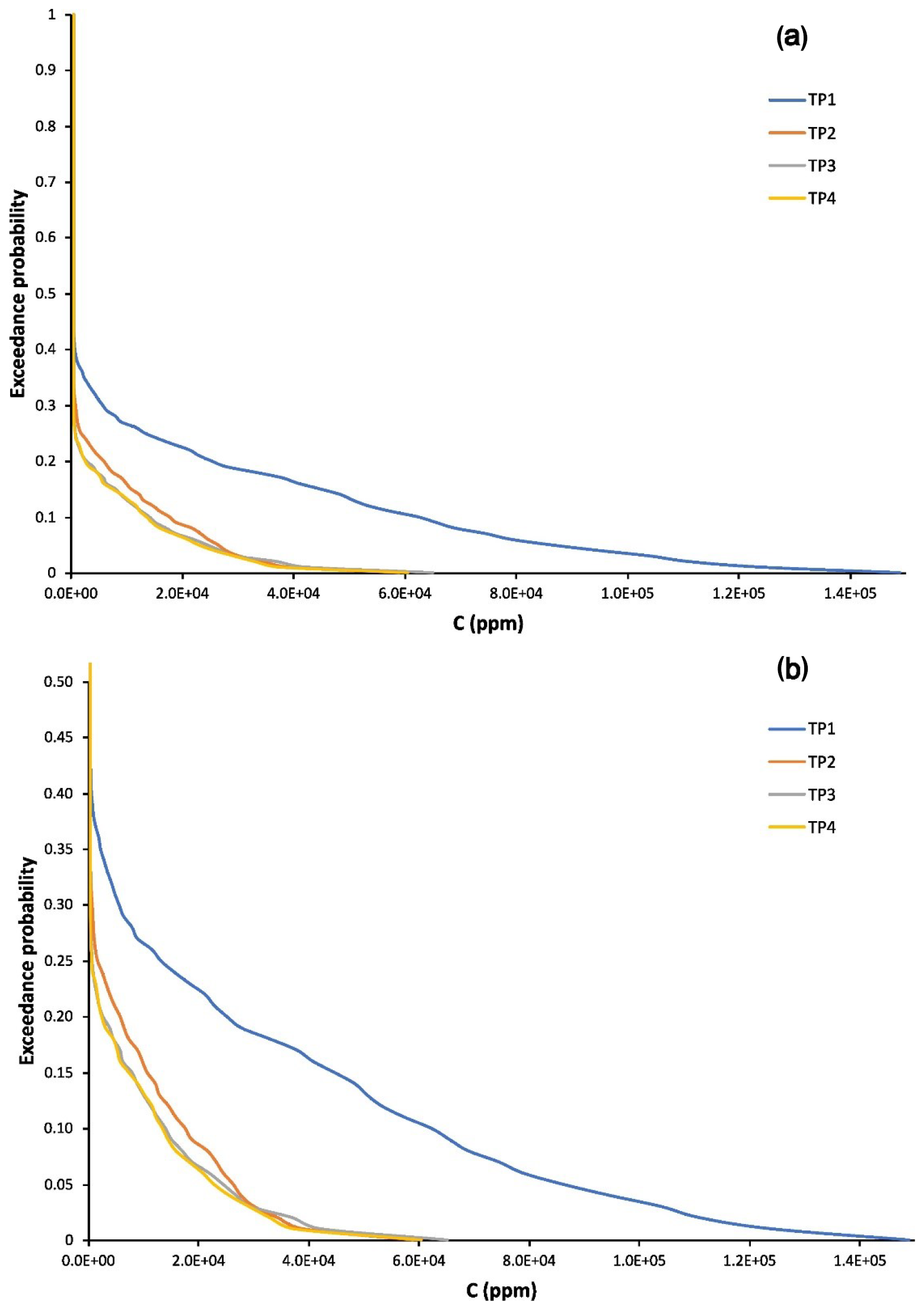
Figure 5 Hazard curves of the 24 h averaged concentration at the four locations identified by the four tracking points. The hazard curves for tracking points 1, 2, 3, and 4 are represented by the solid blue, orange, grey, and yellow lines, respectively. (a) Graph in the original scale used by VIGIL. (b) Zoomed version.

We also wanted to analyse the seasonal control on the simulation outputs, i.e. if the predicted concentrations differ significantly among the four seasons. We first split the dataset of simulations into four categories based on the month of each simulated day: winter (December, January, February), spring (March, April, May), summer (June, July, August), and autumn (September, October, November). For each season, we computed the same outputs (ECDFs and persistence) as those shown in Figs. 3 and 4. In particular, Fig. 6 shows the 24 h time-averaged CO₂ concentration at an exceedance probability of 16 % for the four seasons. The concentrations are significantly higher in the summer season, followed by autumn. Winter and spring are characterised by similarly lower concentrations, although the concentrations are slightly lower in winter than in spring. A closer look at the graphs also shows how the summer is characterised by significantly higher values of CO₂ concentration in the main east–west valley (Fig. 6c), followed by autumn (Fig. 6d). In order to better understand this seasonal control, which according to our hypothesis depends on the wind speeds, we calculated the 24 h time-averaged domain-averaged wind speed at 10 m a.g.l. for each day, and then, by collecting these data for each season, we calculated the ECDF of this averaged wind speed. Figure 7 shows the 24 h time-averaged average wind speed vs. the exceedance probability. Upon first looking at the four curves, it is evident how the wind speed is significantly lower in the summer (solid grey line), followed by the autumn (solid yellow line). The other two seasons display similar trends, although spring (solid orange line) is characterised by lower winds, particularly at exceedance probabilities lower than 50 %. Summarising the findings shown in Fig. 7, higher wind intensities and hence lower concentrations are more likely in winter, followed by spring and autumn. Summer shows the lowest winds and the highest concentrations.

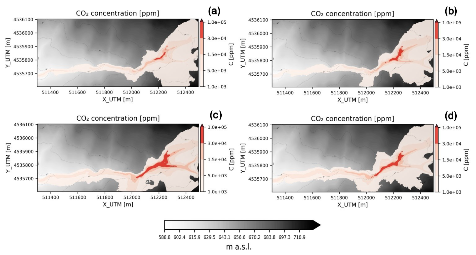
Figure 6 The 24 h time-averaged CO₂ concentration at 2 m a.g.l. at 16 % exceedance probability for the four seasons: (a) winter, (b) spring, (c) summer, (d) autumn.

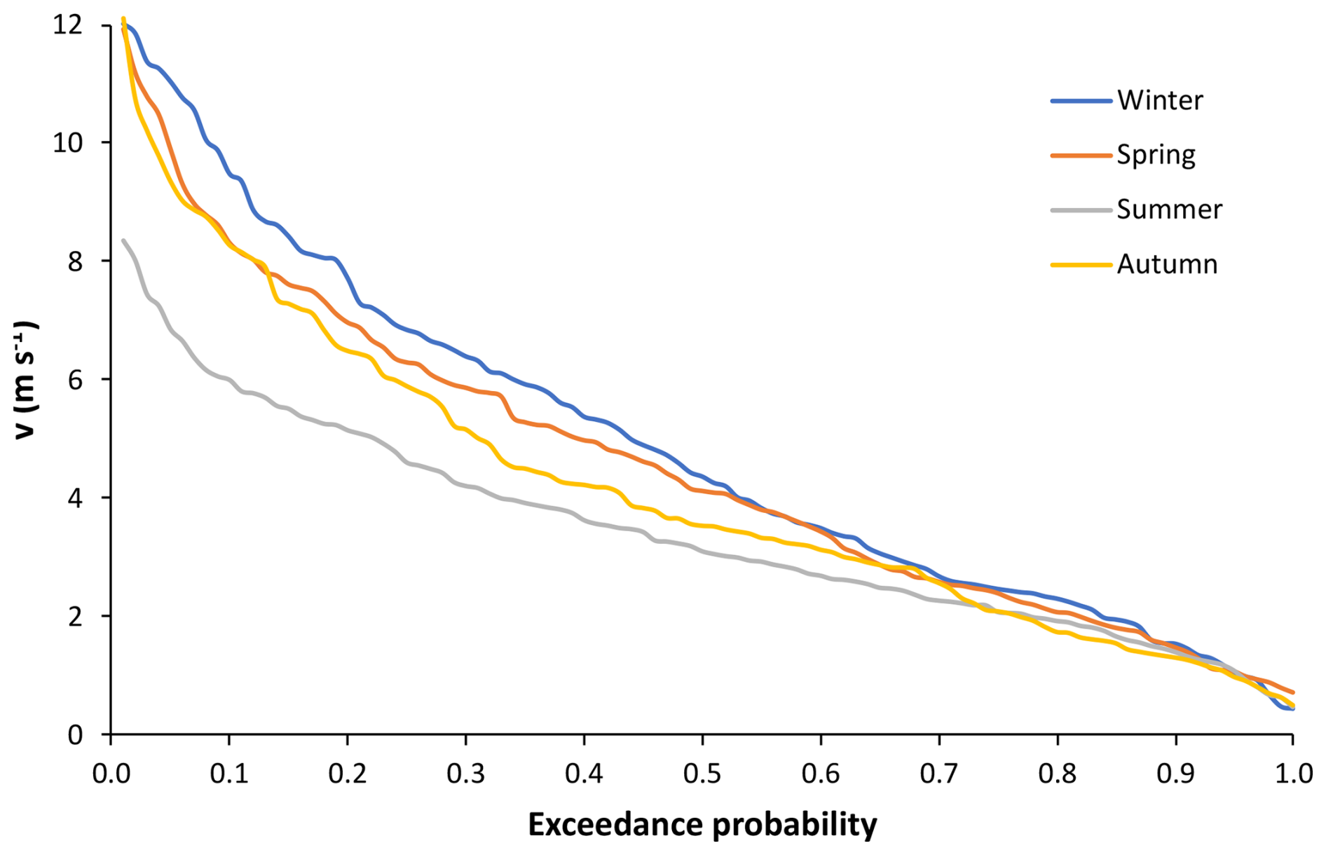
Figure 7 ECDF of the 24 h time-averaged domain-averaged wind speed at 10 m a.g.l. for winter (solid blue line), spring (solid orange line), summer (solid grey line), and autumn (solid yellow line).

It is also worth noting that the probabilities for winds lower than 3 m s⁻¹ are very similar to those for the highest winds (about 12 m s⁻¹), although in the latter case, the summer winds never reach higher than 9 m s⁻¹. The results of the analysis of the meteorological conditions explain the seasonal differences shown in Fig. 6. In the summer, when high winds are less likely than in the other seasons, a dense-gas-flow river is more likely to form in the valleys, with higher concentrations in the areas surrounding the gas source. Autumn shows a similar pattern, although with a slightly lower probability of producing a dense-gas flow in the valleys. This likelihood becomes significantly lower in the autumn and spring. Additionally, the results we are discussing are 24 time averaged. In our view, this is one of the reasons why the effect of wind, which is evident in the seasonal control, prevails over other effects that may dominate in specific time windows of 1 d (e.g. the effect of temperature inversion, which can occur under stable conditions especially in winter and enhances the gas concentration at the lowest levels, may play a role during the night and early morning).

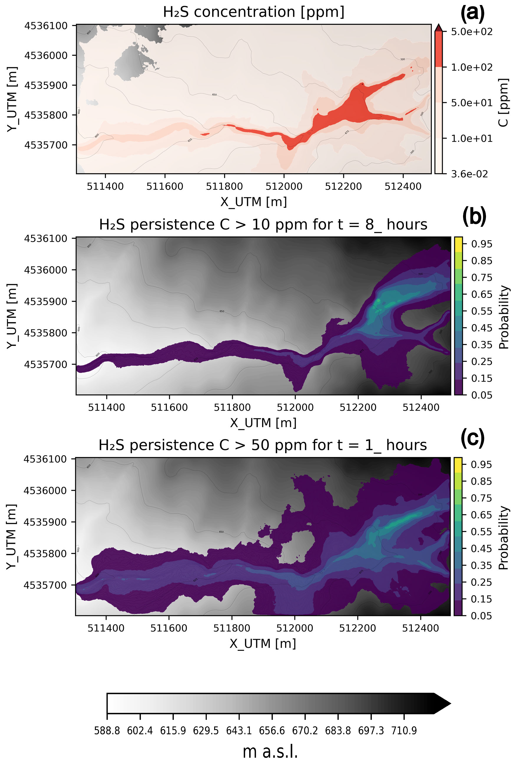
Figure 8 H₂S probabilistic hazard maps at 2 m a.g.l. (a) 24 h time-averaged concentration at 5 % exceedance probability. (b) Persistence maps for PEL 10 ppm with an exposure time of 8 h. (c) Persistence maps for PEL 50 ppm with an exposure time of 1 h.

Finally, Fig. 8 shows some of the probabilistic outputs produced for the H₂S gas species, the concentration thresholds, and exposure times listed in Table 3. The map of H₂S concentration at 2 m a.g.l. at an exceedance probability of 5 % shows levels of H₂S above one of the PELs (>50 ppm) along all the valleys and the emission area. Dangerous levels (>100 ppm) are also significantly widespread in the emission area and the adjacent sectors of the valleys. Figure 8b and c display the persistence maps for two PELs (10 ppm for 8 h and 50 ppm for 1 h; see Table 3). The probability of overcoming these levels for the defined time intervals is significant in the same areas, reaching up to 50 %–60 % in the vicinity of the emission zone for both PELs. The probability of overcoming 50 ppm for 1 h is up to 30 % even 800–1000 m away from the gas source in the main east–west valley. However, we need to highlight the fact that H₂S in the atmosphere tends to react with OH radicals (e.g. Watts, 2000), and other minor sinks can be found on a local scale (e.g. rainfall events and the presence of lakes, soil, and vegetation; Kristmannsdottir et al., 2000; Thorsteinsson et al., 2013; Bussotti et al., 1997; Cihacek and Bremner, 1990). Neglecting such reactions could result in an overestimation of the H₂S concentration, which is probably not significant for our restricted domain. Therefore, whilst further H₂S-specific measurement campaigns are required in order to draw conclusions about the H₂S hazard, these results show that the H₂S hazard should also be taken into account on top of the CO₂ one.

5 Discussion

The analysis carried out with VIGIL confirmed that the computational domain under analysis is prone to non-negligible likelihoods of exposure to high concentrations of CO₂. This is particularly evident in the areas surrounding the gas source and the valleys, especially the main east–west valley where the generation of a cold-CO₂ gas river is a well-known occurrence and is marked by the absence of vegetation at the lowermost levels.

By looking at the 50th percentile of the solutions (50 % exceedance probability of the ECDF generated by VIGIL; Fig. 3), one can observe that, on average, the source area and the area towards the northeast of the emission zone are the most-affected ones, with 24 h time-averaged CO₂ concentrations up to few thousand ppm. The generation of the cold-gas river in the valleys of the domain is observed at lower exceedance probabilities, which implies that this occurrence is less likely. However, the gas river is already quite visible at 16 % exceedance probability, with very high CO₂ concentrations (>15 000 ppm) in many areas in the valleys, source area, and surroundings. This means that there is a 16 % probability of having even worse scenarios, which is not a low likelihood. In fact, at lower exceedance probabilities (5 %), the scenarios look significantly worse. The persistence maps (Fig. 4) created by VIGIL based on the concentration thresholds and related exposure times from Table 2 corroborates these findings. Likelihoods of overcoming dangerous CO₂ concentration levels for specified times are non-negligible to significant. For example, for concentrations of 30 000 and 100 000 ppm, which are dangerous to very dangerous for human health and life even at exposure times of a few minutes, the probability of overcoming these thresholds for 1 h is significant (up to 40 %–50 %), especially in the emission area and the valley segments close to the gas source. It is worth noting that the exposure times for these two concentration thresholds are set to 10–15 min (Table 2), but we were able to calculate the persistence for time intervals of at least 1 h under the current computational limitations, which impose a minimum time step of 1 h. This means that the probabilities shown in Fig. 4d–f would likely be even higher if the proper exposure times (10–15 min; Table 2) had been taken into account. Therefore, our persistence calculation results represent a lower estimate than the real one.

There are similar considerations for H₂S (Fig. 8), whose concentrations in our study were estimated using the gas composition data (Table 1) and the species conversion capability of VIGIL. Results shown in Fig. 8 (H₂S concentration at an exceedance probability of 5 % and persistence maps based on the PEL defined in Table 3) demonstrated that the hazard posed by H₂S cannot be discarded in the area and should be taken into account on top of CO₂ in order to assess the gas hazard in this area.

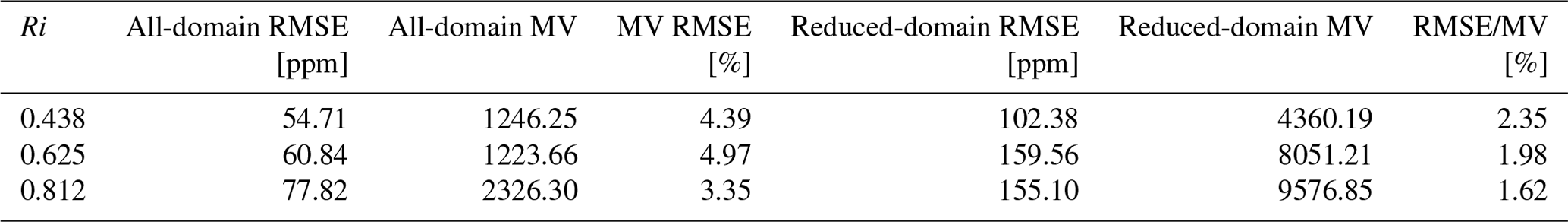
Furthermore, it is worth remembering that in this study, we made use of the new capability introduced in VIGIL v1.3.7, which automatically assigns the gas dispersion scenario based on the Ri value at the source. In the currently implemented approach, a dense-gas scenario is assigned to all the cases in which Ri>0.25 in the intermediate regime ($\mathrm{0.25}<\mathit{\text{Ri}}<\mathrm{1}$); hence, it simulated all these cases with TWODEE-2. This is a cautious choice for the hazard quantification since TWODEE-2 generally results in higher concentrations. The number of simulations in this intermediate regime is 277, which corresponds to 27.7 % of all the simulations; therefore, we conducted an analysis of the outputs produced by the two models in this intermediate regime. Specifically, we selected three simulations with the following values of Ri, chosen to be equally spaced between 0.25 and 1 : 0.438, 0.625, and 0.812. For each case, we conducted the simulation using both DISGAS and TWODEE-2. From the outputs, we calculated the root-mean-square errors (RMSEs) between the DISGAS and the TWODEE-2 solutions in the domain for all the vertical levels and time steps; then we calculated the average of all the RMSEs for each tested case as follows:

$$\begin{array}{}\text{(3)}& \text{RMSE}=\sqrt{{\displaystyle \frac{{\sum }_{i=\mathrm{1}}^N{\left(C_{i,\text{DISGAS}}-C_{i,\text{TWODEE-2}}\right)}^{\mathrm{2}}}{N}}}.\end{array}$$

We then compared the RMSE with the mean value (MV) of the concentration in the domain. Since the RMSE was calculated by comparing the outputs of the two models for each Ri scenario, MV was calculated as follows:

$$\begin{array}{ll}\text{(4)}& {\displaystyle }\text{MV}& {\displaystyle }={\displaystyle \frac{{\text{MV}}_{\text{DISGAS}}+{\text{MV}}_{\text{TWODEE-2}}}{\mathrm{2}}}{\displaystyle }& {\displaystyle }={\displaystyle \frac{\left\{\begin{array}{c}\frac{{\sum }_{i=\mathrm{1}}^N{C}_{i,\text{DISGAS}}}{N}-C_{\text{background}}\\ +\frac{{\sum }_{i=\mathrm{1}}^N{C}_{i,\text{TWODEE-2}}}{N}-C_{\text{background}}\end{array}\right\}}{\mathrm{2}}},\end{array}$$

where C_background is the CO₂ background concentration in the atmosphere (400 ppm). The results are summarised in Table 5 and show that the error is not significant since it is always less than 5 % of the MV. As expected, the discrepancy constantly increases as Ri increases from 55 to 78 ppm. To be further conservative, we considered only the part of the domain where at least one of the two models computed concentration values above the background concentration used in the simulations (400 ppm). In this case, we obtained larger but still not significant RMSE values compared to the MV. These results corroborate our modelling approach in the intermediate regime for this specific case of very high concentrations. Future versions of VIGIL will introduce more robust approaches.

Table 5 Results of the analysis of the influence of selecting either DISGAS or TWODEE-2 in the intermediate Ri regime.

Finally, since DISGAS and TWODEE-2 outputs depend on turbulent diffusion, which in turn depends on the spatial resolution of the computational domain, we carried out a test to verify the dependence of the solution on the chosen spatial discretisation of the domain. Results show that with our settings, the outputs of both DISGAS and TWODEE-2 are not significantly affected by the chosen resolution (see Appendix A).

6 Conclusions

In this work we presented the results of the first PHA carried out at Mefite d'Ansanto, the largest non-volcanic CO₂ gas emission area in Italy and probably on Earth. To do so, we used VIGIL v1.3.7, a Python tool designed to manage the workflow of gas dispersion simulations and post-processing and specifically designed to carry out PHA applications. Thanks to VIGIL, we were able to run 1000 simulations of CO₂ gas dispersion in the area, with each simulation representing the 24 h long dispersion on 1 d randomly sampled from the period of 1 January 1993–1 January 2023. The meteorological data retrieved by VIGIL from the ERA5 dataset (Hersbach et al., 2018a, b) were used to compute the wind field at a high resolution using DIAGNO. Then, for each simulation day, using the new capabilities of VIGIL v1.3.7, we did the following.

• We varied the gas emission rate by randomly sampling it for each simulation from a normal distribution with a mean of 23.1 kg s⁻¹ and a standard deviation of 5.8 kg s⁻¹, according to Chiodini et al. (2010).

• We evaluated the daily averaged Richardson number (thus, neglecting possible intra-daily variations in the Ri number) at the source and based on its value, carried out 24 h long simulations with a 1 h time step using DISGAS or TWODEE-2. In this way, we were not forced to focus on a specific scenario (e.g. the no-wind scenario of Chiodini et al., 2010), to use one of the two models for all the simulations, or to manually select the model to use for each day.

• Finally, the post-processing capabilities of VIGIL allowed us to produce hazard maps, hazard curves, and persistence maps, which highlighted the occurrence of potentially dangerous concentrations of CO₂ at low levels in the atmosphere at non-negligible likelihoods. This is not a surprise, since fatalities have occurred in the past, and the main east–west valley in the domain considered is characterised by a lack of vegetation, which indicates the recurrent occurrence of the cold-CO₂ gas stream. We were also able to obtain preliminary indications of the H₂S hazard in the area, which should not be discarded and should be tackled further in future studies.

We need to stress that this study presents a partial hazard analysis showcasing the new capabilities of VIGIL. A more quantitative hazard assessment, which also accounts for other uncertainties (e.g. the lack of a recent gas emission source characterisation due to the danger and difficulties of field surveys, the use of meteorological data from reanalyses in a fast-evolving climate, etc.) is outside the scope of this paper. However, as recorded by the impacts on the local vegetation and by historical chronicles, the Mefite area is characterised by stable emission rates, similar to those dating back to the Roman era. Therefore, we do not expect significant variation outside the range used in our work, which, in any case, fully includes the statistical uncertainties estimated after the campaigns by Chiodini et al. (2010). Future development of VIGIL will allow better treatment of the uncertainty in the source (in both the location and strength) and assessment of the probability of death depending on the exposure duration, following the approach of Folch et al. (2017), who computed the percentage of human fatalities based on a probability density that depends on concentration thresholds and exposure times of the gas species selected. Furthermore, we plan to use a more up-to-date wind processor that enables time steps shorter than 1 h, which is the current limit due to the use of DIAGNO. This in turn will allow us to improve the analysis of the impact of gas species concentrations on human health since some of the concentration thresholds are related to exposure times of a few minutes. In this way, we should also be able to produce more sophisticated probabilistic outputs of the impacts on human health.

Appendix A: Effect of the computational domain resolution on the modelling outputs

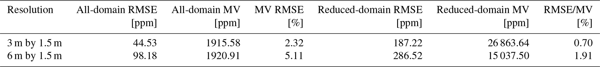
In order to check the effect of the spatial resolution of the discretised computational domain on the modelling output, we carried out test simulations in which we varied the spatial resolution. Specifically, we selected the scenario simulation carried out at Ri=0.438, with a 3 m resolution in the Ri-dependency test from Sect. 5, and carried out two further simulations with spatial resolutions of 1.5 and 6 m. We then calculated the RMSE between the solution at the highest resolution (1.5 m) and the other two solutions (3 and 6 m) using both DISGAS and TWODEE-2:

$$\begin{array}{}\text{(A1)}& \text{RMSE}=\sqrt{{\displaystyle \frac{{\sum }_{i=\mathrm{1}}^N{\left(C_{i\text{,res}}-C_{i{\text{,res}}_{\mathrm{1.5}\mathrm{m}}}\right)}^{\mathrm{2}}}{N}}}.\end{array}$$

Subsequently, we calculated the MV of the concentration obtained with a resolution of 1.5 m:

$$\begin{array}{}\text{(A2)}& \text{MV}={\displaystyle \frac{{\sum }_{i=\mathrm{1}}^N{C}_{i{\text{,res}}_{\mathrm{1.5}\mathrm{m}}}}{N}}-C_{\text{background}}.\end{array}$$

Results for DISGAS and TWODEE-2 are shown in Tables A1 and A2, respectively.

Results show that with the current resolution, the effect of a further refinement is negligible, in particular for DISGAS, which could be expected since DISGAS outputs are less affected by the topography than TWODEE-2.

Table A1 Results of RMSE calculations for the resolution-dependency test for the DISGAS case.

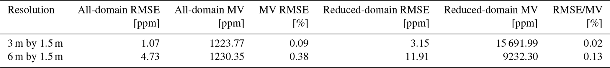
Table A2 Results of RMSE calculations for the resolution-dependency test for the TWODEE-2 case.