Flood exposure of environmental assets

Environmental assets provide important benefits to society and support the equilibrium of natural processes. They can be affected by floods; however, flood risk analyses usually neglect environmental areas due to (i) a lack of agreement on what should be considered an environmental asset, (ii) a poor understanding of environmental values, and (iii) the absence of damage models. The aim of this work is to advance the understanding of environmental exposure to river floods by first identifying asset typologies that could be considered in flood risk analyses and second by introducing a method, named EnvXflood, to estimate flood exposure qualitative values of environmental assets. The method is structured around three levels of detail requiring increasing information, from a fast and minimal-resource analysis suitable for regional assessment to a detailed ecosystem-service-based site analysis. Exposure focuses on the social and environmental value of the assets. Social values were investigated by means of a participatory approach. The method was tested on three case studies in Italy (the Tuscany region, Chiana Basin, and Orcia Basin). The ecosystem service weighting obtained from the participatory approach highlights the perceived leading importance of the biodiversity-supporting service. The results of the analyses show that environmental assets related to water, such as rivers, lakes, and wetlands, are the most exposed to floods. However, they are commonly not considered exposed assets in typical river management practices. Further research should aim at consolidating the asset typologies to be included in environmental exposure analysis and their social and ecological value, moving towards a coherent understanding of environmental flood impacts.

1 Introduction

Environmental assets are crucial for human life, the vitality of ecosystems, and the equilibrium of natural processes. Environmental assets, broadly, are all naturally occurring entities “including those which have no economic values, but bring indirect uses benefits, options and bequest benefits or simply existence benefits which cannot be translated into a present day monetary value” (United Nations, 1993). Among the natural hazards that can impact the environment, river floods have been reported, in the aftermath of recent events, to have affected water resources and water-related ecosystems (Arrighi and Domeneghetti, 2024). Flood influences on environmental assets and their ecosystems, in general, can be expressed as the temporary or permanent alteration of the capability to provide ecosystem services. In particular, one of the main concerns is pollutant transportation by floodwaters (Arrighi et al., 2018; Thieken et al., 2016), which might also increase contaminant concentrations in fishes (Ondarza et al., 2012; Stewart et al., 2003) and destroy habitats (Aldardasawi and Eren, 2021). A recent field study demonstrated that flooding causes more severe and lasting effects on ecosystem processes, including plant productivity and nutrient cycling, compared to droughts (Dodd et al., 2023). Moreover, flooding can cause damages due to the enhanced sediment transport (Weber et al., 2023; Kelman and Spence, 2004) and impacts on aquatic and terrestrial life from temporal turbidity and water quality alteration (Caballero et al., 2024). Floods are reported to also impact on food production (Pacetti et al., 2017), breach and alter riparian zones (Guan et al., 2015), and modify plant reproduction and tree survival (Fischer et al., 2021; Predick et al., 2009), among other things. Nevertheless, potential flood impacts on environmental assets are difficult to understand (Thieken et al., 2016). In fact, for some ecosystems, flooding may represent a regulating natural phenomenon (Natho, 2021), which provides certain habitats with organic and inorganic matter and ensures sustainability and the preservation of biodiversity (Kozlowski, 2002). Concern arises e.g. when, due to anthropogenic pressures, floodwaters transport or resuspend undesired substances, such as contaminants originating from human activities (Barber et al., 1998; Petty et al., 1998; Weber et al., 2023). Assessing the flood exposure of environmental assets has turned out to be useful in many different applications and studies, whether they are aimed at assessing the vulnerability of the assets or the potential positive effects of floods on such natural assets, also taking into account that human activities can strongly influence the flood-regulating capacity of environmental assets (Mori et al., 2021).

The present work is intended to be potentially applied in different areas, but it was developed with the aim to provide an effective instrument for researchers and professionals to fulfil the European requirements in the matter of flood risk assessment.

Indeed, the European Floods Directive requires assessing the potential adverse consequences of floods for the environment and preventing and reducing these impacts. The term environment broadly includes all uses of land, from urban to agricultural, as well as the natural environment. Henceforth, the term environment will refer to the natural environment.

Risk is the probability of a loss, and one of the most widely accepted definitions is based on three elements (Crichton, 1999), i.e. hazard (H), which is a process or a phenomenon threatening the elements at risk; exposure (E) to the hazard, describing the value and location of the elements at risk; and vulnerability (V), which is the extent to which the elements at risk will suffer from damage or loss (Crichton, 1999).

To assess flood risk to environmental assets, given that flood hazard analyses are managed by water authorities and sufficiently detailed for this purpose, one of the most important steps forward is to better describe their exposure to floods. The next step is a vulnerability assessment, which, however, is not covered in this study.

Exposure is commonly quantified by the value or number of assets located in the flooded area (Kron, 2005). Some frequently adopted exposure metrics are the resident population, the number of affected economic activities, the footprint area of the buildings, and their monetary value (Kang et al., 2005) or replacement value (Amadio et al., 2016; Wu et al., 2019; Ye et al., 2019). No standard descriptive metrics are currently commonly accepted and available for environmental heritage and assets, except for their area, and most exposure assessments only report whether the asset is located in a floodable site or not. Moreover, there is no standard agreement on which environmental assets must be included in flood risk management plans. It is believed that the evaluation of environmental assets needs a new approach from researchers (Guijarro and Tsinaslanidis, 2020), aimed at including new elements in the valuation process.

Currently, environmental valuation is usually obtained through different economic instruments, although this is not exhaustive (Gómez-Baggethun and Muradian, 2015; Venkatachalam, 2004).

Environmental valuation can be exploited through the total economic value (TEV) approach, but the specific characteristics of each environmental asset do not allow for uniform treatment with the TEV model (Guijarro and Tsinaslanidis, 2020). Other economic metrics usually applied to environmental evaluation and similar assets (such as cultural heritage) are the “contingent evaluation” method, which encompasses both the “willingness to pay” and the “willingness to accept” approaches (Venkatachalam, 2004), and the “travel cost” method. These methods can eventually be integrated into the final evaluation of environmental assets but only as indicators because they are not able to fully represent the complexity of environmental assets. Issues are also related to the spatial scale of the evaluation because these methods are mainly applicable to small-scale and site-specific studies, but flood risk analyses are often conducted at the watershed or regional scales.

Environmental assets are jointly tangible and intangible assets due to their physical and technical values combined with their cultural, aesthetic, and spiritual values, adding more challenging questions to their proper evaluation. Some experiments aiming to apply a “commodification” of these aspects have been explored (Angeli Aguiton, 2020), but it is believed that the monetization of all the different typologies of environmental assets is utopistic and not representative of reality.

The intangible value also introduces a spatial and temporal variability of the estimate because it is strictly related to the social context and time in which the asset is evaluated.

The study conducted by Robert Costanza (Costanza et al., 1997), titled “The value of the world's ecosystem services and natural capital”, is one of the cornerstones of understanding the value of the environment and makes clear that it is crucial to also focus on the analysis of the ecosystem services that the natural environment can provide to human life. Ecosystems are defined as “a dynamic complex of plant, animal and micro-organism communities and their non-living environment interacting as a functional unit” (emphasis added) by the Convention on Biological Diversity (United Nations, 1992). Ecosystem services can be defined as “the conditions and processes through which natural ecosystems, and the species that comprise them, sustain and fulfil human life” (Ecosystems and their services|Biodiversity Information System for Europe, 2022). As stressed by Costanza et al. (1997), “ecosystem services are largely outside the market”, which elucidates that an approach not closely centred in economic value could be developed and weighted, aiming at providing an evaluating framework that goes beyond the market and that is based on the social and natural value of the environment, which, indirectly, also include the economic aspect. Moreover, despite the diversity of nature's values, most policymaking approaches have prioritized a narrow set of values at the expense of both nature and society, as well as future generations, generally considering only the values of nature reflected through markets and not accounting for the over-exploitation of nature, its ecosystems, and biodiversity and the impact on long-term sustainability (IPBES, 2022).

Examples of studies that identify and assess flood exposure of natural assets (Tait, 2019) are rarely found in the literature, especially when dealing with larger territorial scales, as regional or river basin scales are more typical in risk management plans.

The present work aims to advance the current state of the art in the assessment of flood exposure of environmental assets, with the following specific objectives: (i) develop a taxonomy for environmental assets exposed to flooding, (ii) develop a new non-monetary method for valuing environmental assets that is able to differentiate among asset typologies, and (iii) propose a spatial index of environmental exposure that can support river district authorities in flood risk mapping and management.

The method proposed here is tested and applied to a case study in Italy, where Italian law (Legislative Decree 49/2010) specifically asks to evaluate and manage flood risk for environmental assets and to produce flood risk maps for a list of assets, including environmental assets in areas potentially exposed to floods, but large subjectivity remains in the identification of the assets.

This is a starting point for enhancing the representation of environmental assets while analysing flood risk, also contributing to a more informed risk evaluation and, consequently, better risk management.

2 Materials and methods

2.1 Environmental asset identification and taxonomy

To fulfil objective (i), the first step consists of researching and selecting the assets to be included in the analysis of environmental exposure. In fact, given the diversity of environmental assets and their level of protection, a unique spatial database does not exist and must be created ad hoc by collecting information from different sources. The work starts from UNESCO's definition of natural heritage as “natural places in the world, characterized by their outstanding biodiversity, ecosystems, geology or superb natural phenomena”. But the aim of the work is to consider the meaning of “environmental asset” in its broader connotation, as suggested by the definition reported in the OECD Glossary of Statistical Terms (OECD, 2008), together with the one provided by the United Nations, which considers all naturally occurring entities, “including those which have no economic values, but bring indirect uses benefits, options and bequest benefits or simply existence benefits which cannot be translated into a present day monetary value” (United Nations, 1993). Thus, here we also regard environmental assets as sites which characterize the natural and cultural heritage (mixed sites), landscapes, natural resources, activities, history, and climate of a country or a specific location. Those assets define and influence the characteristics, opportunities, shape, and well-being of neighbouring human settlements and activities. Most environmental assets are identified by international, national, or regional laws, which we used as identification and classification instruments. This approach facilitates the standardization of the procedure over different areas and allows us to identify all the most relevant assets, potentially not including some minor, local assets, which may not be protected or identified by the law. This is in line with the objectives of the present study, especially regarding international-, national-, and regional-scale applications, since minor and less relevant assets have, by definition, less value, with expected low impacts on the final exposure assessment. In the case of studies conducted at catchment scale, or even more local scales (e.g. municipality), specific investigation into the local peculiarities and assets is still suggested, also depending on the capillarity of the local legislation. After identifying the assets commonly protected from international to local levels, a classification of environmental assets has been set, providing a systematic framework for categorizing and understanding the different natural features that may be exposed to flooding. The assets have been grouped according to macro-characteristics and ecosystem typology, enabling a more organized approach to their identification. The different geometric entities required to describe environmental assets in a geographical information system pose an additional challenge in quantifying their exposure with synthetic indices. All the assets identified for the case studies were collected and represented as follows in a GIS environment with different geometric features:

• polygons, in the case of a large portion of territory, such as a forest or a wetland;

• lines, in the case of networks, such as rivers or naturalistic itineraries;

• points, for localized assets, such as a monumental tree or a water spring.

2.2 EnvXflood model structure and levels of analysis

The environmental exposure analysis of the EnvXflood method introduced here is designed to assess the exposure of environmental assets to floods, capturing and qualitatively expressing their value, following objective (ii) of our study. The model has a flexible architecture to be adaptable to different contexts and to be easily integrated with the typical workflows involved in geospatial analysis, with the use of a geographic information system (GIS) and spreadsheets. The core of the estimation framework is the identification and the subsequent evaluation of objective characteristics recognized as belonging to the asset, avoiding direct focus on the economic aspect and instead favouring the ecosystem and social value. The method works both with the legislative framework and with ecosystem services delivered by the identified assets. Ecosystem services are powerful instruments capable of describing natural capital and its relations with human beings and their activities (Chen et al., 2022; Liu et al., 2024), recently gaining a growing interest and consideration from the scientific community. After the identification and classification of the asset, the following step regards the weighting of the features attributed to each asset. Among the results, there is the overall environmental exposure index (EEI), as detailed in the following paragraphs, to achieve objective (iii) of the work.

The method is designed to work at different spatial scales and with different degrees of detail and information. This structure enables us to perform the assessment at national or international scales, where the ecosystem service association may be unevenly feasible across the area, thus relying only on the laws and the official documentation provided by the authorities. This is the most basic and flexible level of the analysis, namely level 1. When the assessment is focused on smaller scales, e.g. regional or watershed, the assets are further classified with an enriched taxonomy, also including the ecosystem services associated with the defined assets (level 2 of the framework), thus providing a more accurate representation of their value. When instead the assessment aims to describe local flood exposure of environmental assets, e.g. at watershed and municipality scales, a deeper, specific analysis is requested, adding a more detailed, case-study-specific list of the ecosystem services associated with the environmental assets in the area (level 3). Level 2 and level 3 are designed to include insights from a participatory-based approach. A graphic schematization of the proposed framework is reported in Fig. 1. The framework is incremental, so the assessment always starts with a level-1 analysis, adding information incrementally before reaching level-2 or level-3 detail. Step 0 is the collection of the assets in the study area, thus building a dataset of environmental assets, represented in the figure by the blocks with a dashed perimeter. The dataset may be enriched and updated while moving through the analysis levels. Step 1 is to determine the listing relevance of the assets, as better described in Sect. 2.2.1, thus creating the updated taxonomy for level 1. After the level-1 weighting procedure (see Sect. 2.2.1), the flood hazard information is added to the analysis, thus determining the environmental exposure index (EEI) of level 1. Moving to the second level of the analysis, the assessment follows the level-1 taxonomy, which is now enriched with the ecosystem services, thus creating the updated level-2 taxonomy (see Sect. 2.2.2). After the level-2 weighting procedure, the flood hazard information is added, and the level-2 EEI is obtained. The same workflow applies for level 3 (Sect. 2.2.3).

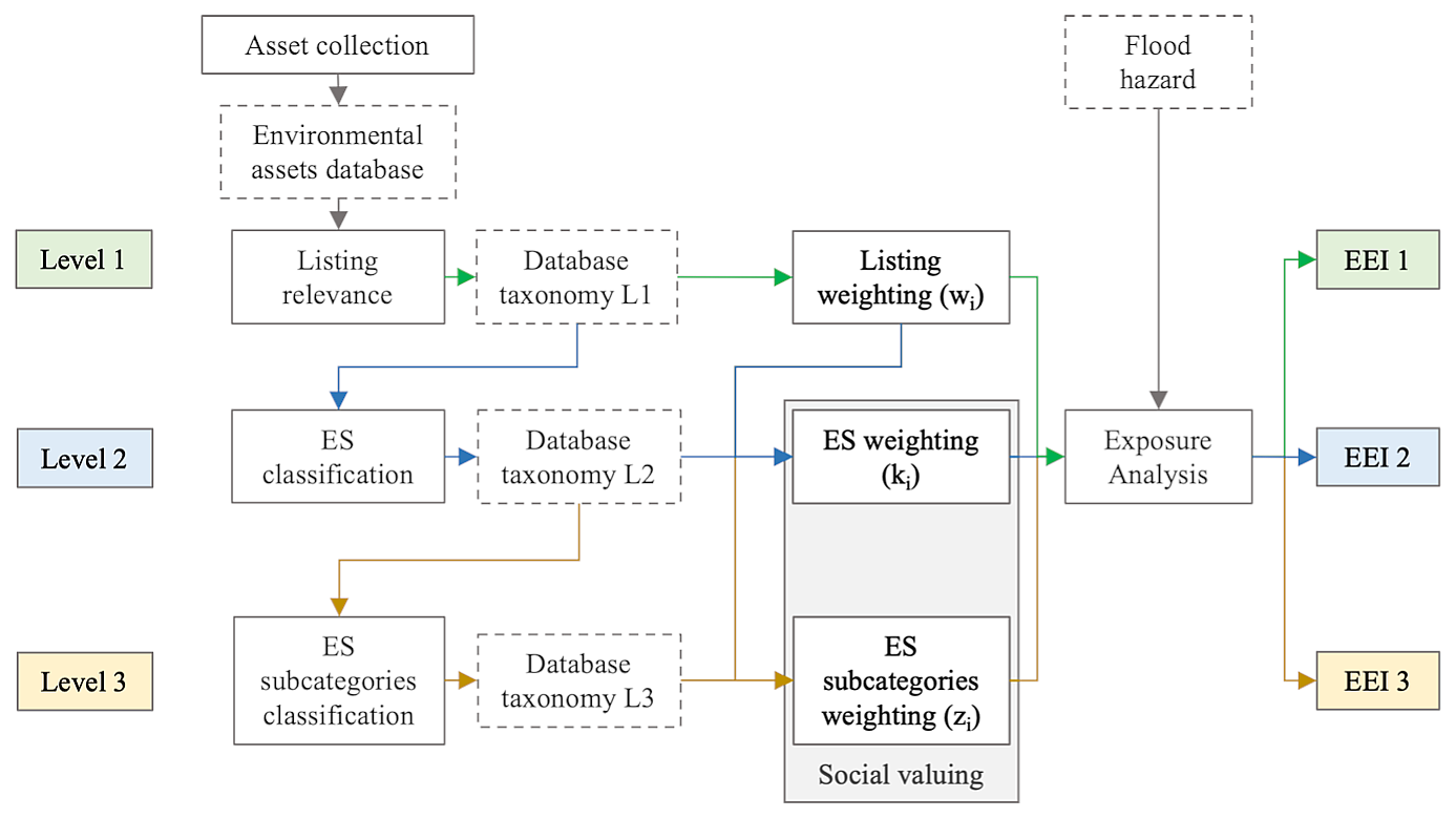
Figure 1 EnvXflood methodological workflow for the determination of the environmental exposure index (EEI) at the three levels of analysis. Ecosystem service is abbreviated as ES.

In this methodological framework, several variables are defined. The environmental asset value EV_i,l is the weighted value of the ith asset in the level of analysis l, where $l=\left\{\mathrm{1},\mathrm{2},\mathrm{3}\right\}$, obtained through a min–max normalization of the weights. Therefore, EV_i,l expresses the value attributed to an asset category, given the level of analysis. The variable ${\stackrel{\mathrm{‾}}{n}}_{i,l}$ is defined for each analysis level and represents the weight assigned to asset i.

$$\begin{array}{}\text{(1)}& {\displaystyle }& {\displaystyle }\text{Level 1: }{\text{EV}}_{i,\mathrm{1}}={\displaystyle \frac{n_{i,\mathrm{1}}-min\left(n_{i,\mathrm{1}}\right)}{max\left(n_{i,\mathrm{1}}\right)-min\left(n_{i,\mathrm{1}}\right)}}\text{(2)}& {\displaystyle }& {\displaystyle }\text{Level 2: }{\text{EV}}_{i,\mathrm{2}}={\displaystyle \frac{n_{i,\mathrm{2}}-min\left(n_{i,\mathrm{2}}\right)}{max\left(n_{i,\mathrm{2}}\right)-min\left(n_{i,\mathrm{2}}\right)}}\text{(3)}& {\displaystyle }& {\displaystyle }\text{Level 3: }{\text{EV}}_{i,\mathrm{3}}={\displaystyle \frac{n_{i,\mathrm{3}}-min\left(n_{i,\mathrm{3}}\right)}{max\left(n_{i,\mathrm{3}}\right)-min\left(n_{i,\mathrm{3}}\right)}}\end{array}$$

A description of the weights is given in Sect. 2.2.1–2.2.3.

An equivalence factor (EqF) is defined to determine equivalent units (areas or lengths or numbers, depending on the asset's geometry type) of the assets, based on their value EV_i, and is obtained by adding a unit to the environmental asset value EV_i,l. Thus, one unit of the most important asset is equivalent to two units of the least important asset, greatly simplifying the understanding of the results obtained by the proposed valuing methodology. The EqF provides a reference asset value (e.g. the least important or the most important), thus enhancing the interpretation and delivery of the results.

The environmental asset exposure value EEV_i,l expresses the exposure of the assets to the flood:

$$\begin{array}{}\text{(4)}& {\text{EEV}}_{i,l}={\text{EV}}_{i,l}\times e_{\text{f}},\end{array}$$

where e_f is the exposed fraction, i.e. the percentage of exposed area with respect to the total asset area for polygon features, the percentage of exposed length with respect to the total asset length for line features, and the percentage of the exposed number of assets with respect to the total number of assets for point features. When EEV_i,l is calculated on a study area, it highlights the most significant environmental asset exposed, i.e. the most inundated and the most valuable.

While the above EV_i and EEV_i refer to a single ith asset category, the overall environmental exposure index (EEI) for the study area, which includes multiple asset categories, is defined as the sum of all the values of the asset categories, as it follows

$$\begin{array}{}\text{(5)}& {\text{EEI}}_l=\sum _{i=\mathrm{1}}^n{\text{EEV}}_{i,l},\end{array}$$

where n is the number of the assets considered in the analysis.

The value of the EEI represents a flood exposure score which allows for making comparisons among catchments or territories to identify the most exposed areas and assets.

Finally, the ratio of the EEI to the sum of the values of the assets present in the area is defined as the exposed environmental fraction (EEF) and describes, in percentage, the exposed value with respect to the maximum total value (EV) of the assets in the area. This is an additional indicator that allows us to rapidly compare the exposure of different study areas and the significance of flood exposure with respect to the overall environmental asset value of the study area.

$$\begin{array}{}\text{(6)}& {\text{EEF}}_l={\displaystyle \frac{{\text{EEI}}_l}{{\sum }_{\mathrm{1}}^n{\text{EV}}_{i,l}}}\end{array}$$

The method developed in this study can be applied with different input datasets, but it will produce different results if the input features are not the same among the analyses. Thus, for each study, it is important to carefully select the characteristics to be used as descriptors of the assets to ensure that they are uniform and fully retrievable for all areas of interest.

It is pointed out that analyses carried out at different levels are not comparable, having different evaluation features and weights, thus changing the evaluation algorithm.

2.2.1 Level 1

The first level (Eq. 1) is the fastest to be implemented and requires determining the relevance of the assets, based on the level of listing (local, regional, national, international). International listing includes UNESCO environmental heritage but also other assets protected by supranational agreements, such as the Ramsar Convention on Wetlands. Level 1 can be easily applied at large scales, and thus it can be suitable for regional/catchment analysis needed in flood risk management plans. The spatial database of level 1 includes the listing level according to the available information regarding protecting laws/conventions or recognitions. A weight w_i is assigned to each asset such that for each step the weight is doubled, starting from 1 for local (i.e. municipal, provincial), then 2 for regional, 4 for national, and 8 for international assets; i.e. $w=\left\{\mathrm{1},\mathrm{2},\mathrm{4},\mathrm{8}\right\}$. For example, an asset falling under the UNESCO, Ramsar, or Natura 2000 listings, which are international identifications, will be assigned a weight equal to 8, i.e. the maximum weight. National parks, for instance, are instead usually protected by national laws, and the assigned weight will be 4. A weight equal to 2 will be assigned to regional parks and all the other assets individuated only by regional authorities. Some municipalities or provinces will identify some other assets that are relevant only at a local scale. A minimum weight of 1 will be assigned to these assets.

2.2.2 Level 2

The second level of analysis (Eq. 2) includes the social value of the environmental asset category, expressed as the people's perception of the importance of the ecosystem services commonly associated with that asset category. Among the different ecosystem service classifications, we refer to the one provided by the Millennium Ecosystem Assessment (MEA, 2005), in which there are four categories: supporting, provisioning, regulating, and cultural. In the following we refer to these as the “main” ecosystem service categories, and we assign to them an index j, where $j=\mathit{\{}\mathrm{1},\mathrm{2},\mathrm{3},\mathrm{4}\mathit{\}}$ such that j=1 is for supporting ESs, j=2 is for provisioning ESs, j=3 is for regulating ESs, and j=4 is for cultural ESs. For each asset category (e.g. forests), a review is performed to find existing studies regarding the ES related to it, thus building a list of ecosystem services associated with each environmental asset category. Where it was not possible to find specific studies, the analysis was based on expert judgement. In the example of forests, it is usually recognized that they provide supporting, provisioning, regulating, and cultural services. Another general example could be the one of viewpoints, regarded as environmental assets that provide only cultural ESs.

All the information was eventually collected in a spatial database for the level-2 taxonomy.

For computational simplicity, the information regarding the ecosystem services provided by each asset category was translated into a matrix $\stackrel{\mathrm{‾}}{\mathbf{P}}$, (n×j) with zeroes and ones, with ones meaning that the corresponding ecosystem service is provided and zeroes meaning the opposite.

To distinguish among the j ecosystem service categories introduced above, weights were assigned to them. Assigning weights to ecosystem services is a common procedure in environmental decision-making, like in multi-criteria decision analysis (Adem Esmail and Geneletti, 2018), especially when the goal is to establish a ranking among those services. Weighting helps resolve trade-offs between conflicting ecosystem services, such as provisioning (e.g. food production) and regulating services (e.g. carbon sequestration). The significance of weighting lies in its ability to translate in a simple and effective manner how various ecosystem services are valued. The column vector P contains the four p_j weights assigned to the ES categories, which can be determined by running a survey, as was done in this study and described in Sect. 2.2.4.

In summary, the ${\stackrel{\mathrm{‾}}{p}}_{i,j}$ elements of the matrix $\stackrel{\mathrm{‾}}{\mathbf{P}}$ are thus equal to 1 when the jth ES is attributed to the ith environmental asset and 0 when not. Then, multiplying $\stackrel{\mathrm{‾}}{\mathbf{P}}$, (n×j) for the ecosystem service weights in the column vector P will assign to each environmental asset category their partial weight, k_i. To obtain the final weight for the level-2 analysis, ${\stackrel{\mathrm{‾}}{n}}_{i,\mathrm{2}}$, k_i needs to be multiplied by the listing level from level 1, w_i.

$$\begin{array}{}\text{(7)}& {\displaystyle }& {\displaystyle }\stackrel{\mathrm{‾}}{\mathbf{P}}={\stackrel{\mathrm{‾}}{p}}_{i,j}=\left\{\begin{array}{l}\mathrm{1}\Rightarrow {\text{ES}}_j\in E_i\\ \mathrm{0}\Rightarrow {\text{ES}}_j\notin E_i\end{array}\right.\text{(8)}& {\displaystyle }& {\displaystyle }{k}_i=\stackrel{\mathrm{‾}}{\mathbf{P}}\times \mathit{P}\text{(9)}& {\displaystyle }& {\displaystyle }{\stackrel{\mathrm{‾}}{n}}_{i,\mathrm{2}}=k_i\times w_i\end{array}$$

Here, ${\stackrel{\mathrm{‾}}{n}}_{i,\mathrm{2}}$ is the final weight assigned to each asset category in the level-2 procedure, which is used in Eq. (2) to determine the environmental value EV_i,2 for level 2.

2.2.3 Level 3

The third level of the analysis (Eq. 3) adds a further classification of environmental assets to create a level-3 taxonomy and assign the weights z_i (Eq. 10).

For each main category of ecosystem services (supporting, provisioning, regulating, cultural), a sub-set of four classes of ecosystem services was selected to be able to identify with more accuracy the properties and the differences of the assets and to improve the analysis' alignment with reality. Such classes are representative of the most common ESs for each category, as listed for instance in the Millennium Ecosystem Assessment (MEA, 2005; Reid et al., 2005).

They are organized in the array ES_sub, (j×s) as shown in Fig. 2 for a total of m=16 ecosystem service subcategories.

Figure 2 Graphical representation of the structure of the ecosystem service subcategories.

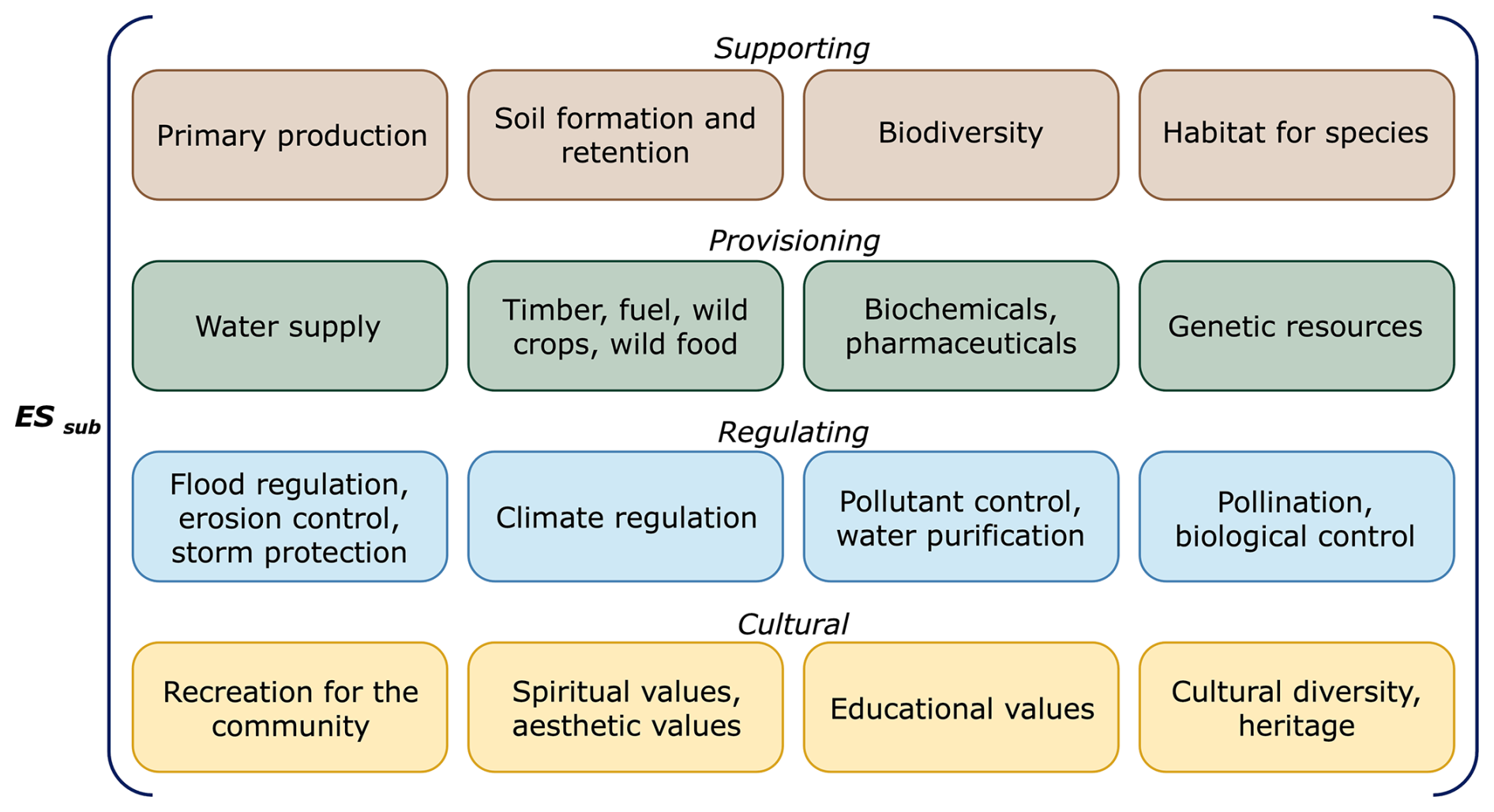
The index j of the rows represents the corresponding main ES categories, which are the same as those defined for level 2. This third level of analysis is intended for the study of smaller areas due to the high detail of classification needed. Specific studies or ad hoc local expert panels can help in defining local environmental assets and in assigning weights to different ecosystem service subcategories. In this work the ES subcategory weights sw_j,s are assigned based on the survey (Sect. 2.2.4) and stored in the matrix ${\stackrel{\mathrm{‾}}{\mathbf{S}}}_{\mathrm{w}}$, (j×s), with the same structure as ES_sub.

The matrix S is then defined as the product of P_diag, which stores the weights p_j of the four main ES categories (the same as level 2) and the matrix S_w of the ES subcategory weights.

$$\begin{array}{}\text{(10)}& {\displaystyle }& {\displaystyle }\mathbf{S}={\mathbf{P}}_{\text{diag}}\times {\mathbf{S}}_{\mathrm{w}}\text{(11)}& {\displaystyle }& {\displaystyle }{\mathbf{P}}_{\text{diag}}=\text{diag}\left(p_j\right)\end{array}$$

Similarly to as described for level 2, the matrix $\stackrel{\mathrm{‾}}{\mathbf{S}}$, (n×m) of zeroes and ones stores 1 if an mth ES subcategory is attributed to the ith asset and allows us to apply the ES subcategory weights selectively to only the assets which provide those ESs. Thus, the elements ${\stackrel{\mathrm{‾}}{s}}_{i,m}$ of the matrix $\stackrel{\mathrm{‾}}{\mathbf{S}}$ are equal to 1 when the mth ES subcategory is attributed to the ith environmental asset and are otherwise 0.

$$\begin{array}{}\text{(12)}& \stackrel{\mathrm{‾}}{\mathbf{S}}={\stackrel{\mathrm{‾}}{s}}_{i,m}=\left\{\begin{array}{l}\mathrm{1}\Rightarrow {\text{ES}}_{{\text{sub}}_m}\in E_i\\ \mathrm{0}\Rightarrow {\text{ES}}_{{\text{sub}}_m}\notin E_i\end{array}\right.\end{array}$$

Eventually, the partial z_i (Eq. 10) weights are assigned to each asset, and they can then be used in Eq. (3).

$$\begin{array}{}\text{(13)}& z_i=\stackrel{\mathrm{‾}}{\mathbf{S}}\times {\mathit{S}}_{\mathrm{c}}\end{array}$$

Here, the column vector S_c, (m×1) is obtained by arranging the elements of S in a single column, row by row.

$$\begin{array}{}\text{(14)}& {\stackrel{\mathrm{‾}}{n}}_{i,\mathrm{3}}=k_i\times w_i\times z_i\end{array}$$

Eventually, ${\stackrel{\mathrm{‾}}{n}}_{i,\mathrm{3}}$ in Eq. (14) represents the weight of an asset in the level-3 analysis, and it is used to determine the environmental value in EV_i,3 in Eq. (3).

2.3 The survey

The survey was developed by means of the Google Forms web platform (supplementary material), targeting a group of individuals familiar with environmental and flood-related topics but not necessarily experts in ecosystem services or environmental assets. The targeting choice is based on the rationale of acquiring insights from people able to fully understand the proposed questions but without limiting the audience to only environmental experts. Different and multiple targeting is possible, and the results may eventually be aggregated into one. This participatory approach follows a basic but effective version of methodologies commonly used in multi-criteria decision-making analysis (MCDM/A), already proven to be meaningful and suitable for flood risk assessment (Evers et al., 2018; Hansson et al., 2013) and, more broadly, in similar sectors (Ferla et al., 2024), where stakeholder input is essential for capturing complex and broad-ranging relationships, here with the objective of determining priority in environmental management and protection. The survey asks people to rank the ES category (for the level-2 classification) and subcategories (for the level-3 classification) from the most to the least important. The weights $w=\mathit{\{}\mathrm{1},\mathrm{2},\mathrm{3},\mathrm{4}\mathit{\}}$ are assigned as the following: the highest weight, 4, goes to the first classified, and the lower weight, 1, goes to the last. To identify the degree of consensus among respondents, a decimal value representing the proportion of responses (s=share) that selected each category was appended to the assigned weight. This approach retains information about the share of participants who selected each option, providing insight into the uncertainty or variation in public opinion regarding the importance of each category. For example, following Eq. (15), if a category has been voted as the second most important (second = weight 3) by 50 % of the respondents (share=0.50), its sw_j,s weight for the matrix $S_{\mathrm{w}},(j\times s)$ in Eq. (10) would be 3.5:

$$\begin{array}{}\text{(15)}& {\text{sw}}_{j,s}=w+s,\end{array}$$

where w is the raw weight derived from the pure ranking, and s is the share of the responses, as described above.

2.4 Case studies: Tuscany, Italy

The study area for applying levels 1 and 2 of the analysis is the Tuscany region in central Italy (Fig. 3a and b). Tuscany extends for about 23 000 km², and its morphology includes mountain chains and some plains, but it is dominated by hills, which occupy approximately 66 % of the area. Its main river is the Arno River, which has a length of about 241 km and a catchment area of about 8288 km².

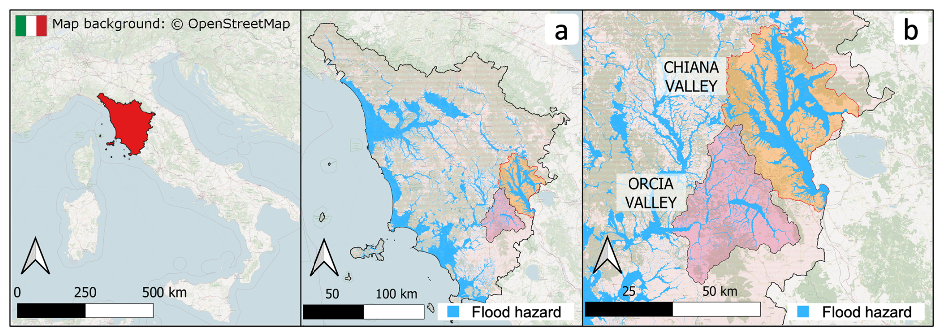
Figure 3 Case study identification. The Tuscany region for levels 1 and 2 (a); the Chiana and Orcia valleys for level 3 (b). Flood hazard areas are depicted in blue (flood hazard extent: Autorità di bacino distrettuale dell'Appennino Settentrionale). Map background: © OpenStreetMap contributors 2023. Distributed under the Open Data Commons Open Database License (ODbL) v1.0.

Only the portion of the regional area managed by the Northern Apennines River Basin District Authority, which covers approximately the whole region, is included in the present study.

For the analysis of level 3, two catchments in the region are selected to compare the results: the Orcia and the Chiana valleys (Fig. 3c).

The Orcia Valley is in the south-east of the Tuscany region and took its name from the Orcia River, which has a length of about 57 km, flows from east to west, and has an overall watershed surface area of about 798 km², considering the basin delineation named Sant'Angelo-Cinigiano in the dataset provided by the Tuscany regional authority for hydrology (SIR). A portion of the valley has been inscribed in the UNESCO World Heritage Sites since 2004 for its landscape's distinctive aesthetics.

The Chiana Valley is morphologically flatter than the Orcia Valley, and its main drainage canal is the Canale Maestro della Chiana, which is a 62 km length artificial channel flowing from south to north. The watershed surface area is about 1290 km². Many attempts of reclamation have been made in the past since ancient times, and they eventually resulted in the completion of the Canale Maestro della Chiana and its network of tributaries. The channel starts near Lake Chiusi, and it is a left tributary of the Arno River. The confluence is located near the city of Arezzo. The Chiana Valley watershed area studied here is a sub-basin of the Arno River basin, identified by the name Ponte Ferrovia FI-Roma in the basin delineation provided by the Tuscany regional authority for hydrology (SIR).

The list of environmental assets included in the spatial database for the whole Tuscany and for the Orcia and Chiana valleys is available as supplementary material, and all the information has been retrieved from public datasets of the official authorities at regional, national, and international levels (Bertoli et al., 2025).

2.5 Flood hazard

The hazard assessment was carried out with the official flood hazard maps made available according to the European directives 2000/60/CE and 2007/60/CE, provided by the Autorità di bacino distrettuale dell'Appennino Settentrionale, within the Flood Risk Management Plan (FRMP) (PGRA, 2025). The maps were employed in the study to assess the flood extent and thus the areas directly exposed to the flood hazard. The maps refer to three hazard levels: P1 is the low hazard level, P2 is the medium hazard level, and P3 is the high hazard level. The analysis was based on the low-probability hazard scenario, P1.

3 Results and discussions

3.1 Environmental asset taxonomy

Figure 4 summarizes the environmental assets considered and collected to create the baseline geospatial database. The proposed taxonomy, as already introduced, has initially been defined taking advantage of the most relevant international laws for environmental asset conservation and protection. It is divided into four macro-categories, embracing all the collected assets. They are the following:

• water resources and ecosystems

• geologic sites

• terrestrial ecosystems

• landscapes.

Figure 4 Taxonomy of the most relevant environmental assets, categorized into (i) water resources and ecosystems, (ii) geologic sites, (iii) terrestrial ecosystems, and (iv) landscapes.

Intermediate categories have been defined for each macro-class, providing a more transferable taxonomy, which include freshwater bodies, coastal areas and transitional waters, landforms, underground geosites, fossil-bearing layers, wildlife sanctuaries, parks, terrestrial habitats, land scenery, sightseeing spots, and trails. The last branches of the scheme are populated by the specific environmental assets that we were able to identify. While moving among different areas, the onomastics may vary, and some adaptation may be necessary, though most of the assets can be represented or included in the proposed list.

Water bodies, wetlands (e.g. RAMSAR areas), rivers, and lakes are explicitly considered in the flood exposure analysis carried out in this work, highlighting their relevant involvement in floods. Despite this, they are usually excluded from common flood impact and risk analyses as water bodies, adopting overly strong simplifications that are no longer adequate to correctly represent the phenomenon.

3.2 Survey results

The survey received about 65 answers. A total of 63 % of them were provided by students, researchers, and professionals in the field of water and environmental sciences and engineering.

Table 1 reports the weights to be used in the level-2 and level-3 analyses, resulting from the processing of the survey's answers.

Table 1 Weights applied to the ES categories, resulting from the survey. At level 2, the main ES categories are shown. At level 3, the respective subcategories are reported.

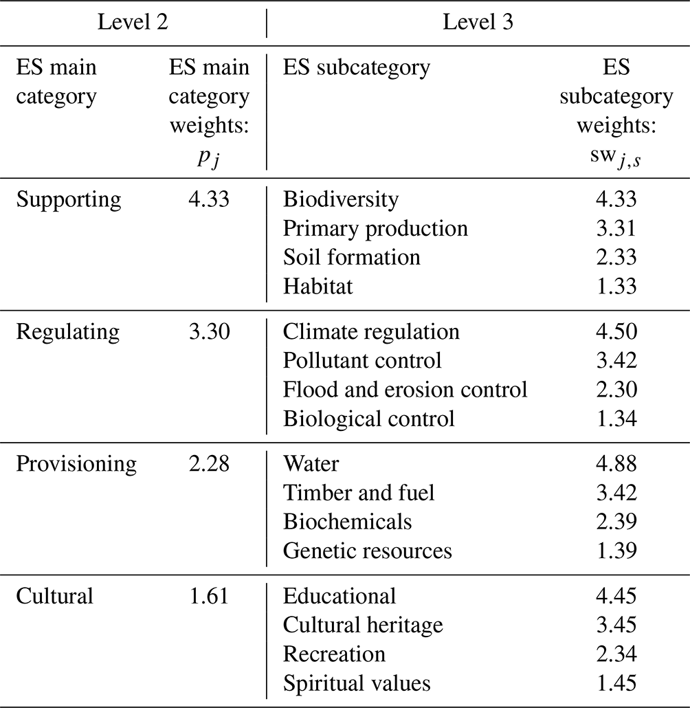
The supporting ES category turned out to be the most important. Among its ES subcategories, biodiversity is placed first, followed by primary production, soil formation, and habitat. The share of the answers, expressed by the decimals of the weights, was around 30 % for all the choices, indicating a homogeneous distribution of the answers. The regulating ES category resulted in the second most important ES main category. Among its ES subcategories, climate regulation was voted the most important, with a good degree of accordance (50 %). The provisioning ES ranked third among the main ESs, and the water subcategory was voted first, with a high degree of accordance (88 %). The last main ES was the cultural one, with an accordance of 61 %, and the most important subcategory was the educational one.

Due to the nature of the topic, it is considered appropriate to potentially open the survey to a wider range of expertise, including, for example, biologists, economists, and cultural heritage experts. Local and regional stakeholders could furthermore be involved, aiming to reach a better policy impact and making the analysis as suitable as possible to the study area. The selected weights should be the most shared possible; however, they remain related to the social, historical, and environmental context and time in which the assets are evaluated and are strictly dependent on the scale of the project. It is relevant to point out that the framework of the EnvXflood method can also work with different sets of weights, and it is also possible to perform parallel analyses of the same areas, applying different weights. This allows for comparison of the environmental assets' exposure to floods, for instance, from two or more different points of view, such as the ones of different stakeholders, creating seminal comparative results for decision-making processes and the authorities.

3.3 Tuscany region results

The methodology, as already discussed, was designed to work with three levels of analysis. The different insights obtained through the three levels make it possible to perform very rapid (level 1) yet meaningful analyses in the case of post-disaster assessments of assets hit by a flood, as well as very detailed evaluations (level 2, level 3) that are more suitable to prevention and planning measures, thus making this framework adaptable to multiple necessities and different scenarios. The second level of analysis is well balanced among resources (time, data) and results obtained, and it could be effectively applied at regional scales. The third level requires carrying out site-specific studies during all phases of the analysis, implying a considerable amount of time and resources. It is more suitable for applications at small scales, like protected areas and sub-basins (e.g. valleys).

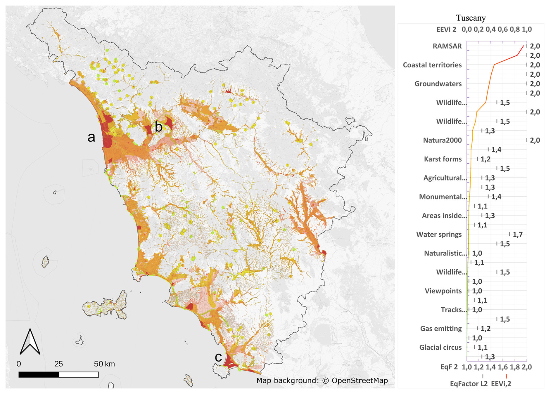
Figure 5 Flood exposure of the environmental assets in the Tuscany region, with the most exposed environmental assets shown in red, progressively grading to yellow and green, depending on their ranking in the level-2 analysis. The areas with high-exposure values marked with a, b, and c represent Lake Massaciuccoli, Fucecchio swamps, and the Orbetello Lagoon respectively. Map background: © OpenStreetMap contributors 2023. Distributed under the Open Data Commons Open Database License (ODbL) v1.0.

In this study, the method developed was applied to the Tuscany region in Italy. The level-1 and level-2 analyses were performed for the whole region. Figure 5 reports the most significant results of the second-level analysis. The figure is composed of a map on the left and a diagram on the right, which also represents the legend for the colour ramp adopted in the map. The environmental asset flood exposure value (EEV_i,2) is plotted on the top axis of the diagram, and it is graphically represented by the colour-graded line (from red (most exposed) to green (less exposed)). The equivalence factor (EqF) is plotted on the bottom axis of the chart, graphically represented in the diagram by the vertical grey segments. This set of information already provides a complete view of the analysis of the assets, expressing how significant the assets are (EqF), and the weighing scale between their value and their physical exposure to the hazard (EEV_i), i.e. the flood.

Table 2 Resulting indicators of the level-2 analysis carried out for the Tuscany region.

The overall environmental exposure index, EEI₂, and the exposed environmental fraction, EEF₂, are reported in Table 2. The equivalence factor, EqF_i, and the exposed environmental value, EEV_i, are designed for a comparison among the assets within the study area, while EEI₂ and EEF₂ are intended for a comparison among different but similar areas, as far as they are homogeneous in the data availability. The total environmental value (EV₂) obtained in the analysis is also reported on the map.

The EEF indicator provides a direct and very effective reading of the flood exposure of the assets of the region, which, for the Tuscany region, is about 33 %. The EEF is a large-scale indicator, useful for comparisons among different areas, but to detail the knowledge of the flood exposure of the assets in the area, it is necessary to focus on the environmental exposure value (EEV_i) of each asset. Water-related assets are, as expected, ranked first. This means that they are the most valuable assets and the most flooded assets too. This result must not be taken for granted, and it is strongly believed that it is necessary to include water-related assets in flood risk assessments, since often they are not. Assessing their exposure to floods provides important information about the knowledge of the territory and the hazard, allowing better responses in the event of need (e.g. pollution spread, physical damages, and habitat or ecosystem losses).

The most exposed assets are the RAMSAR areas, followed by lakes (coloured in red in Fig. 5, such as Lake Massaciuccoli highlighted by “a”, the Fucecchio swamps highlighted by “b”, and the Orbetello Lagoon highlighted by “c”), the coastal territories, and the lake buffer areas (in dark orange in Fig. 5). Groundwaters (in this study considered the footprint of the aquifer recharge) and rivers are in the fifth and sixth positions respectively. From this point on, the two rankings (level 1 and level 2) become distinct because the differences in the EV computed in the two analyses are more pronounced. In level 1, not reported here, the EV is only guided by the level of protection, i.e. legislative listing. In contrast, in level 2, the ESs provided by the assets are also included to describe their importance at an ecosystem, an environmental, and a social level, thus providing a different, more significant ranking. A good exemplification could be the one of the mountain bike (MTB) tracks: they are listed at the regional level, thus ranking 14th out of 34 in the level-1 analysis. In level 2, they are recognized to provide only a few ESs (cultural); thus, despite the regional listing, they fall to the end of the ranking, leaving the higher places to the most important assets (assets providing more ecosystem services).

From a scientific and engineering point of view, to know which assets are more exposed to floods than others and in a way being able to identify the role of assets in the ecosystem and in society, therefore getting a measure of their value, is a great step forward. This result opens new perspectives in the management of flood risk. Firstly, aligning environmental exposure analysis outcomes to the common exposure definition used in risk analyses, such as buildings' exposure, makes it possible to integrate the environmental assets' exposure into conventional risk equations. Furthermore, using ecosystem services as part of the evaluation guarantees a holistic approach to the issue, rather than focusing only on a single aspect of it. Secondly, this mode of assessing flood exposure enables a smoother transition to the next research phases (e.g. vulnerability assessments), straightforwardly prioritizing the most exposed assets and creating the conditions necessary for rapid growth in research and significant improvements in flood risk assessments for environmental assets. Advancements should then focus on the environmental assets' vulnerability to floods, explicitly considering the peculiarities of floods in the Anthropocene.

Returning to the map, reporting the equivalence factor along with the EEV aims to stress the social, environmental, and – indirectly – economic values expressed through the ESs provided by the assets, which are included in the EEV. The most valuable assets have the highest EqFs, and most of them are ranked first. Nevertheless, other valuable assets, like the Natura 2000 and UNESCO assets, are not exposed as much as RAMSAR or lake assets, thus ranking lower in the EEV ranking because they are less flooded. This exemplifies well how the model is capable of ranking the assets efficiently while keeping all the important aspects in the computations. The areal extension of the environmental assets exposed to floods in the Tuscany region is clearly reported in Fig. 4. In the map the exposure extension of the coasts and the coastal territories of Tuscany is also observable, which are almost completely highly exposed to floods.

3.3.1 Orcia Valley and Chiana Valley results

For the Orcia and Chiana valleys, the analysis was pushed to the third level, thus including more details about the ecosystem services provided by the assets. Figures 6 and 7 report the main outcomes. The figures are composed of the same elements described in the previous section. The environmental asset exposure value (EEV_i,3) is plotted on the top axis of the diagram, and it is graphically represented by the colour-graded line (from red (most exposed) to green (less exposed)). The equivalence factor (EqF), plotted on the bottom axis of the chart, is also graphically represented in the diagram by the vertical grey segments. The overall environmental exposure index, EEI₃; the exposed environmental fraction, EEF₃; and the environmental value, EV₃, are reported in Table 3.

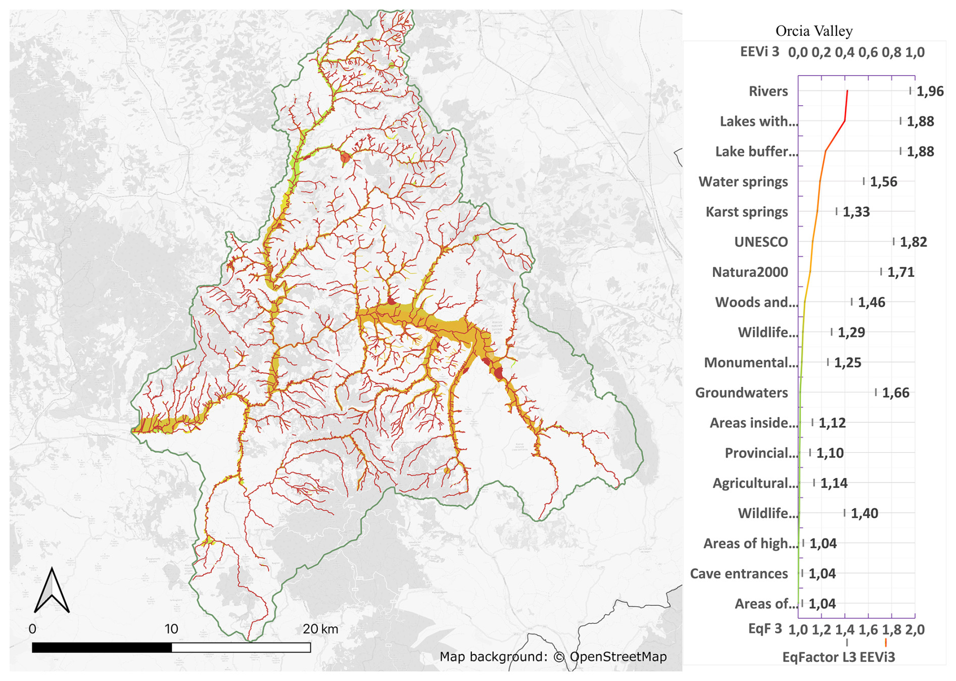
Figure 6 Flood exposure of the environmental assets of the Orcia Valley. The most exposed environmental assets are in red, progressively grading to yellow and green, depending on their ranking from the level-3 analysis. Map background: © OpenStreetMap contributors 2023. Distributed under the Open Data Commons Open Database License (ODbL) v1.0.

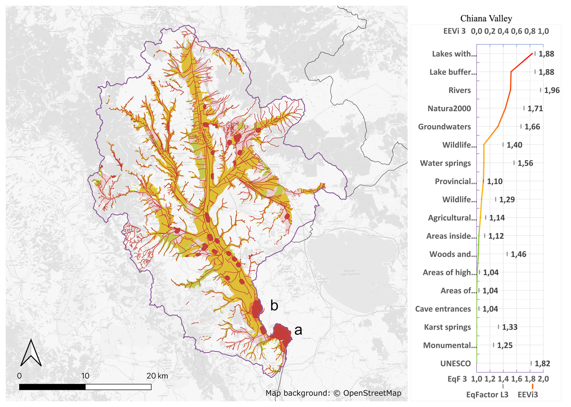
Figure 7 Flood exposure of the environmental assets of the Chiana Valley. The most exposed environmental assets are in red, progressively grading to yellow and green, depending on their ranking from the level-3 analysis. Highlighted are Lake Chiusi (a) and the Nature Reserve of Lake Montepulciano (b). Map background: © OpenStreetMap contributors 2023. Distributed under the Open Data Commons Open Database License (ODbL) v1.0.

Table 3 Resulting indicators of the level-3 analysis carried out for the Orcia and Chiana valleys.

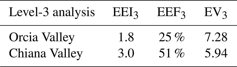
The results of the level-3 analysis performed for the Orcia and Chiana valleys are fully comparable. These outcomes can be used by regional authorities to prioritize further studies, focusing on assessing the flood vulnerability of the most exposed assets and areas, eventually planning mitigation measures where they are most necessary, and effectively minimizing environmental and social losses. It is evident from analysis outcomes that the environmental assets of the Chiana Valley are more exposed to floods than those in the Orcia Valley. The Chiana Valley is morphologically flatter than the Orcia Valley, and it also presents other characteristics which favour flooding. It also has several lakes and wet areas, as highlighted in red in Fig. 7, and the drainage network is largely artificial. Two major lakes are located to the south, Lake Chiusi (Fig. 7a) and Lake Montepulciano, which is also a natural reserve (Fig. 7b). In contrast, the Orcia Valley has a very dense drainage network (Fig. 6) and only a few lakes. The analysis pointed out that the environmental value (EV) of the Orcia Valley is greater than that of the Chiana Valley (Table 3) since, for instance, UNESCO assets are not present in the Chiana Valley, such as monumental trees, karst springs, and cave entrances. However, the environmental exposure fraction (EEF) and the EEI index of the Chiana Valley are approximately double those of the Orcia Valley due to greater flood extension. Thus, even if the value of the assets is lower, the indicators show that the environmental assets' exposure to floods is higher in the Chiana Valley. The EqF values become particularly effective in this comparison, highlighting significant assets which are not largely flooded but deserve more attention in the analyses due to their environmental value. This is the case for UNESCO and Natura 2000 assets in the Orcia Valley. The EqF can be a guide for further asset-specific analyses to better assess the exposure and, eventually, flood risk of the most important assets.

Overall, rivers are the most exposed assets in the Orcia Valley, followed by lakes and their buffer areas, water, and karst springs. Regarding the Chiana Valley, the most exposed assets are lakes, their buffer areas, rivers, the Natura2000 areas, and groundwaters. The Chiana Valley lakes have almost double the exposure value compared to those in the Orcia Valley. Even if ranked third, rivers have a higher exposure value (proportionally) in the Chiana Valley than in the Orcia Valley due to the reasons discussed above.

Natura 2000 assets are present in both valleys, and they are more exposed in the Chiana Valley.

4 Discussion and conclusions

Flood risk assessment of environmental assets is a process that currently lacks fundamentals, such as shared and effective definitions and methodologies to assess their exposure and vulnerability to flooding. This study aimed to provide an environmental asset taxonomy (research objective i), which has been defined as taking advantage of the most relevant international laws for environmental asset conservation and protection. The proposed taxonomy was then integrated with more detailed environmental asset categories, defined from the ones already present in the European and Italian legislative frameworks and adapted with intermediate categories to enhance its transferability without limiting its application to the case study examined in the present work. This taxonomy can help researchers and practitioners to properly recognize environmental assets to be included in flood risk analyses and can be adapted to fit local peculiarities if required. The four main categories, i.e. water resources and ecosystems, geologic sites, terrestrial ecosystems, and landscapes, are wide-ranging and also easy to apply in different settings without needing further adaptations. The second step of the study was the development of a method, named EnvXflood, to estimate flood exposure of environmental assets (research objective ii), delivering the overall environmental exposure index (EEI) (research objective iii). Exposure assessment focuses on the social and environmental value of assets, beyond the flooded area analysis, also through the evaluation of the ecosystem services provided by each environmental asset category. Social values were investigated by means of a participatory approach. The methodology developed in this study is structured across three levels of detail requiring increasing information, from fast analyses suitable for regional assessment (level 1 and level 2) to a detailed ecosystem-service-based site analysis (level 3). The method outcome is the ranking of the environmental assets, ordered from the most important and most flooded to the least important and least flooded. The application of the method to the study area in Italy (Tuscany region – Chiana and Orcia basins) highlighted that the environmental assets related to water, such as rivers, lakes, and wetlands, are the assets most exposed to floods and among the most valuable in terms of ecosystem services provided. Despite this, water bodies are often neglected in flood risk analysis under the assumption that flooding does not cause damage to natural areas and thus do not require a sound and comprehensive flood risk analysis. This assumption is no longer considered acceptable since human activity has deeply changed natural areas, and many aspects are emerging from studies on potential impacts (Arrighi and Domeneghetti, 2024). During and after a flood, ecosystem service delivery is altered and may be disrupted for a certain amount of time (Dodd et al., 2023), the habitat provisioning service may be interrupted (Ciampittiello et al., 2022), and pollutants may be transported with effects on ecosystems and health (Weber et al., 2023). Extreme floods can significantly alter aquatic ecosystems and the ecosystem services they provide (Talbot et al., 2018).

Moreover, flood impacts on the biodiversity of terrestrial animals have been assessed, with the severity depending on various factors, such as flood duration and depth (Zhang et al., 2021), but due to anthropogenic alterations, floods also affect the biodiversity in riverine systems (Walker et al., 2022). Additionally, floods significantly impact lake ecosystems by altering their hydrological characteristics and affecting water quality, salinity, and biological processes (Muduli et al., 2022). Further research should aim at consolidating asset taxonomies for flood exposure analysis and their social value, moving towards a consistent understanding of environmental flood impacts. Moreover, a standardized procedure for the weighting process and standardized databases of environmental assets officially made available by authorities would represent improvements, effectively fostering comparison among regions, even if they are controlled by different administrations. This work was developed to be a first step forward towards a better, more informed, and more comparable flood exposure assessment of environmental assets and, consequently, a better flood risk assessment. Scientific communities and authorities working at any spatial scale strongly need commonly accepted procedures and shared knowledge to improve the research on and the management of environmental assets, and the outcomes of this work aim to fill this current gap. Indeed, as it is a novel approach in a field not well documented by the literature, it includes some uncertainties, especially regarding weight selection. While the individuation of the environmental asset categories relies on laws and official datasets, the weights represent the opinion of the interviewed people regarding the importance of the ecosystem services associated with the assets. The results reflect the diverse social, economic, educational, and professional backgrounds of the respondents, as well as their personal experiences and the local context in which they reside. Despite this diversity, the derived weights are still considered robust and accurately represent the relative importance of ecosystem services (ESs) and their roles, in line with the structured participatory approach based on multi-criteria decision-making analysis (MCDM/A) methodologies (e.g. Evers et al., 2018; Ferla et al., 2024; Hansson et al., 2013). While future surveys or expert consultations could provide further refinements, especially if applied to areas in which the social context is vastly different from the one of our audience, significant variations from the current findings are not anticipated. Slight variations are also expected when changing the professional background of the audience, as well as when moving to the industry sector or to a wider, generalized, and less informed public, e.g. residents. Nevertheless, additional expert validation in the participatory approach is recommended to enhance the robustness and reliability of the results.

Another source of uncertainty is the partial subjectivity included in the attribution of the ecosystem services to the environmental assets, which, wherever possible, was based on the literature, with some inclusion of expert opinion when necessary.