Multi-scale hydraulic graph neural networks for flood modelling

Deep-learning-based surrogate models represent a powerful alternative to numerical models for speeding up flood mapping while preserving accuracy. In particular, solutions based on hydraulic-based graph neural networks (SWE-GNNs) enable transferability to domains not used for training and allow the inclusion of physical constraints. However, these models are limited due to four main aspects. First, they cannot model rapid differences in flow propagation speeds; secondly, they can face instabilities during training when using a large number of layers, needed for effective modelling; third, they cannot accommodate time-varying boundary conditions; and fourth, they require initial conditions from a numerical solver. To address these issues, we propose a multi-scale hydraulic-based graph neural network (mSWE-GNN) that models the flood at different resolutions and propagation speeds. We include time-varying boundary conditions via ghost cells, which enforce the solution at the domain’s boundary and drop the need for a numerical solver for the initial conditions. To improve generalization over unseen meshes and reduce the data demand, we use invariance principles and make the inputs independent from coordinates' rotations. Numerical results applied to dike-breach floods show that the model predicts the full spatio-temporal simulation of the flood over unseen irregular meshes, topographies, and time-varying boundary conditions, with mean absolute errors in time of 0.05 m for water depths and 0.003 m² s⁻¹ for unit discharges. We further corroborate the mSWE-GNN in a realistic case study in the Netherlands and show generalization capabilities with only one fine-tuning sample, with mean absolute errors of 0.12 m for water depth, a critical success index for a water depth threshold of 0.05 m of 87.68 %, and speed-ups of over 700 times. Overall, the approach opens up several avenues for probabilistic analyses of realistic configurations and flood scenarios.

1 Introduction

Precise flood models are invaluable for evaluating risks, issuing early warnings, and improving preparedness against flood events. Two-dimensional hydrodynamic models determine the spatio-temporal evolution of floods by solving the shallow-water equations (SWEs) (Teng et al., 2017). To address the intensive computational demands required to solve the SWEs, we can resort to several strategies, such as using simplified physical models (e.g. Van den Bout et al., 2023) and high-performance clusters (e.g. Caviedes-Voullième et al., 2023). More recently, deep learning models have emerged as an in-between option that can accelerate flood simulations while maintaining high accuracy (Bentivoglio et al., 2022). Most deep learning models predict the flood evolution or its maximum depths while generalizing over different boundary conditions, such as rainfall, on a single domain. These models include transformers (Pianforini et al., 2024), convolutional neural networks (CNNs) (Berkhahn and Neuweiler, 2024; Liao et al., 2023; Kabir et al., 2020; Guo et al., 2021; He et al., 2023), graph neural networks (GNNs) (Burrichter et al., 2023), Fourier neural operators (Xu et al., 2024), and long short-term memory (LSTM) networks (Wei et al., 2024). Although these methods are effective over a given area, they must be trained again when applied to a different domain, thus hindering their use as surrogate models.

As such, research is now focusing on generalizing deep learning flood models to unseen case studies that the models were not trained on. For example, Löwe et al. (2021), Guo et al. (2022), and Cache et al. (2024) proposed CNN models to estimate the maximum water depth of pluvial floods in urban and catchment settings, respectively. A conditional generative adversarial network to predict the maximum water depth for unseen rain events and urban catchments was developed by do Lago et al. (2023, 2024). Bentivoglio et al. (2023) proposed a hydraulic-based graph neural network (SWE-GNN) that could predict the spatio-temporal evolution of dike-breach floods over unseen topographies. The main advantages of this model are its link with finite-volume methods that makes it suitable to simulate the physics on meshes and a hydraulic-based propagation rule that enforces continuity in water propagation. Moreover, compared to previous works, it can also predict the full flood's spatio-temporal evolution. However, the model cannot reproduce very different propagation speeds and needs a high number of layers when simulating large time steps, which can make the training process unstable. Moreover, this approach uses a fixed boundary condition and requires the first time step to be given by a numerical solver.

To overcome these limitations, we propose a multi-scale hydraulic graph neural network, based on an SWE-GNN. Multi-scale models combine the domain information coming from different resolutions and have shown benefits for simulating other partial differential equations (Lino et al., 2022; Fortunato et al., 2022). To drop the dependency from the numerical solver, we integrate time-varying boundary conditions via ghost cells, i.e. mesh cells that receive a known value of a given variable at the domain boundary (LeVeque, 2002). To improve the generalization to unseen meshes, we remove all coordinate-dependent inputs. This makes the model invariant to rotations (Bronstein et al., 2021); that is, rotations of the inputs do not affect the outputs. This helps because it prevents the direction of flooding from being biased towards a specific direction in the training data.

We validate the model on dike-breach flood simulations over non-squared domains, discretized by irregular meshes and with different topographies and time-varying boundary conditions. To test the applicability of this model to real-world case studies, we consider a flood scenario for the breaching of a levee system in the Netherlands.

The key novelties of this paper can be summarized as follows:

• We develop a multi-scale approach which improves the simulations in both speed and accuracy, with speed-ups of up to 1000 times and mean absolute errors of 0.05 m and 0.003 m² s⁻¹ for water depth and unit discharges, respectively.

• We include time-varying boundary conditions via the use of ghost cells to remove the dependency from the numerical models, and we improve generalization to unseen meshes by making the model's inputs invariant to rotations.

• We show that the model generalizes well to a realistic case study with a bigger area and wider range of boundary conditions than the training ones, with only one fine-tuning simulation.

The rest of the paper is organized as follows: in Sect. 2, we give an overview of the methods – we describe the mesh creation process, introduce the multi-scale hydraulic graph neural network model, describe how to include boundary conditions via ghost cells, detail the inputs and outputs of the model, and present the training loss function. Then in Sect. 3 we describe the synthetic and case study datasets, and we present the results in Sect. 4. We discuss the method in Sect. 5 and conclude in Sect. 6.

2 Methodology

We developed a multi-scale graph neural network that combines the information at progressively coarser resolutions to propagate floods in space and time with different flow speeds (Fig. 1). As input the proposed model takes static features that represent the topography and connectivity of the domain at different resolutions and dynamic features that represent the hydraulic variables at time t. It then processes them via a U-shaped architecture that applies graph neural networks at different scales and combines them with downsampling and upsampling operators. The outputs are the predicted hydraulic variables at the following time step t+1 at the finest available resolution. We added boundary conditions by assigning a known value of water depth or discharge to a set of cells at the domain boundary.

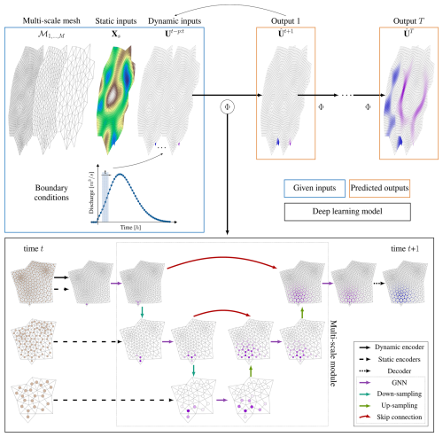
Figure 1 Overview of the proposed mSWE-GNN model. As input the model Φ(⋅) takes a fine mesh and its coarser versions, along with the static and dynamic inputs defined on them (blue box, top left) and produces an estimate of the hydraulic variables in time (orange box, top right). The model is then repeated auto-regressively using its predictions as inputs (top black arrow) to determine the spatio-temporal evolution of the flood. Boundary conditions are provided at each time step by assigning a known value to a set of cells in the dynamic inputs ${\mathbf{U}}^{t-p:t}$. In the black box, black arrows indicate multi-layer perceptrons (MLPs) present in the encoders and the decoder; purple arrows represent graph neural network layers; light-green arrows represent downsampling layers; dark-green arrows represent upsampling layers; and red arrows skip connections across different parts of the architecture.

In the following, we detail the multi-scale mesh creation procedure (Sect. 2.1) and the model architecture (Sect. 2.2). Then we show how to include boundary conditions (Sect. 2.3) and rotation-invariant inputs (Sect. 2.4). Finally, we describe the employed loss function (Sect. 2.5). We denoted variables x at a given scale or resolution ℳ_m as $x^{\cdot ,m}$, where ⋅ is a placeholder for other indices and where the variable can be a scalar x, a vector x, a matrix X, or a tensor 𝒳. When the superscript m is omitted, we refer to the variables at the finest scale.

2.1 Multi-scale mesh creation

We designed a multi-scale model that combines meshes with progressively coarser resolutions. We employed an iterative process that requires only the boundary polygon of a selected area without any prior knowledge of the underlying topography. First, we create a coarse mesh from a boundary polygon using the MeshKernel software (Deltares, 2024). This corresponds to the mesh in the bottleneck of the multi-scale module (Fig. 1). Then we refine the mesh by splitting each mesh edge in two and connecting the newly formed points via edges. Next the mesh undergoes an iterative orthogonalization algorithm needed for the underlying numerical software Delft3D to run because of its staggered grid scheme (Deltares, 2022). For the same numerical constraints, after the orthogonalization, all elongated elements are removed, resulting in a mixture of triangular and quadrilateral elements. We define elongated elements as those whose line connecting the barycentre and edge middle points is 0.1 times smaller than the other lines in the same element. We repeat these steps multiple times depending on the required scale of computations in the fine mesh. The obtained set of meshes constitutes our multi-scale mesh.

2.1.1 Multi-scale graph

The computational graph used in the proposed model considers the barycentres of the mesh cells to be nodes, while edges connect neighbouring cells. We connect the graphs at two scales based on the spatial position of the mesh barycentres, as shown in Fig. 2. If a fine mesh cell's centre is within a coarse mesh cell centre, then a directed inter-scale edge exists between the two nodes.

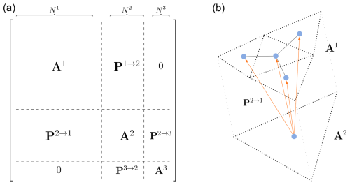
Figure 2 (a) Adjacency matrix representation of the multi-scale graph for a mesh with three scales. ${\mathbf{A}}^m\in {\mathbb{R}}^{N^m\times N^m}$ represents the adjacency matrix at scale m, while ${\mathbf{P}}^{m\to n}\in {\mathbb{R}}^{N^m\times N^n}$ represents the prolongation matrix from scale m to scale n. (b) Example connection between a fine mesh A¹ and a coarse mesh A², where P^2→1 indicates the connectivity across the two scales.

We can describe the connectivity of the obtained multi-scale graph via a block-diagonal connectivity matrix composed of adjacency matrices A^m and prolongation matrices P^m→n. Adjacency matrices are squared matrices that represent the connectivity of a graph at scale m by assigning $a_{ij}^m=\mathrm{1}$ if edge (i,j) exists. Prolongation matrices are rectangular matrices that act like adjacency matrices but connect one scale m to its upper or lower scale $n\in \mathit{\{}m+\mathrm{1},m-\mathrm{1}\mathit{\}}$. They can also be seen as adjacency matrices for bipartite graphs whose nodes can be divided into two disjoint sets.

2.2 Architecture

We develop a multi-scale hydraulic graph neural network (mSWE-GNN) by building upon Bentivoglio et al. (2023). This is an encoder–processor–decoder architecture that auto-regressively predicts the hydraulic variables at time t+1 as

$$\begin{array}{}\text{(1)}& {\widehat{\mathbf{U}}}^{t+\mathrm{1}}={\mathbf{U}}^t+\mathrm{\Phi }({\mathbf{X}}_{\mathrm{s}},{\mathbf{U}}^{t-p:t},\mathcal{E}),\end{array}$$

where the output ${\widehat{\mathbf{U}}}^{t+\mathrm{1}}$ corresponds to the predicted hydraulic variables; U^t denotes the hydraulic variables (water depth [m] and unit discharge [m² s⁻¹]) at time t; Φ(⋅) is an encoder–processor–decoder model that determines the evolution of the hydraulic variables for a fixed time step; X_s denotes the static node features; ${\mathbf{U}}^{t-p:t}$ denotes the dynamic node features, i.e. the hydraulic variables for time steps t−p to t; and 𝓔 denotes the edge features that describe the geometry of the mesh. We include different mesh resolutions by defining the model Φ(⋅) in a U-shaped architecture, inspired by Gao and Ji (2019), starting from a fine mesh and going to coarser ones and back to a fine mesh output. Hereafter, we describe the details of the architecture shown in Fig. 1.

2.2.1 Encoder

We increase the expressivity of the inputs by employing three separate encoders for processing the static node features ${\mathbf{X}}_{\mathrm{s}}\in {\mathbb{R}}^{N\times I_{\mathrm{s}}}$, the dynamic node features ${\mathbf{X}}_{\mathrm{d}}\equiv {\mathbf{U}}^{t-p:t}\in {\mathbb{R}}^{N^{\mathrm{1}}\times O(p+\mathrm{1})}$, and the edge features $\mathcal{E}\in {\mathbb{R}}^{E\times I_{\mathit{\epsilon }}}$, with N being the total number of nodes, I_s the number of static node features, N¹ the number of nodes at the finest scale, O the number of hydraulic variables, p the number of input previous time steps, E the number of edges, and I_ε the number of input edge features. The encoded variables are defined as

$$\begin{array}{}\text{(2)}& {\mathbf{H}}_s={\mathit{\varphi }}_s\left({\mathbf{X}}_{\mathrm{s}}\right),{\mathbf{H}}_d={\mathit{\varphi }}_d\left({\mathbf{X}}_{\mathrm{d}}\right),{\mathcal{E}}^{\prime }={\mathit{\varphi }}_{\mathit{\epsilon }}\left(\mathcal{E}\right),\end{array}$$

where ϕ_s(⋅) and ϕ_d(⋅) are three-layer MLPs shared across all nodes, $\mathbf{H}\in {\mathbb{R}}^{N\times G}$ denotes the encoded node features, and ϕ_ε(⋅) is a three-layer MLP shared across all edges that encodes the edge features into ${\mathcal{E}}^{\prime }\in {\mathbb{R}}^{E\times G}$, with G being the number of features in the latent space. The encoded variables H_s, H_d, and 𝓔^′ represent a higher-dimensional version of the original inputs that is more expressive. We apply the shared encoders of the static features ϕ_s(⋅) and ϕ_ε(⋅) to all features at all scales, while the encoder of the dynamic features ϕ_d(⋅) is applied only to the finest scale. The rationale behind having a shared static feature encoder for all scales is that higher-dimensional features should have similar embedding independently of the scale, since the physical quantities are the same.

2.2.2 Processor

The processor propagates the encoded inputs throughout the multi-scale graph. We employ a sequence of GNN layers to propagate information at a given scale and connect two scales via downsampling and upsampling operators. The operations are organized in a U-shaped fashion, with a downsampling branch from fine to coarse and an upsampling branch from coarse to fine, as shown in Fig. 1.

In the downsampling branch, we start by applying L GNN layers at the encoded node and edge features ${\mathbf{H}}_s^{\mathrm{1}}$, ${\mathbf{H}}_d^{\mathrm{1}}$, and ${{\mathcal{E}}^{\prime }}^{\mathrm{1}}$ at the finest-scale mesh ℳ₁. Then we apply a downsampling operator $\downarrow :{\mathcal{M}}_m\to {\mathcal{M}}_{m+\mathrm{1}}$ that maps the features of the finer scale ℳ_m to the coarser scale ℳ_m+1. We repeat these two operations until reaching the final coarser scale. In the upsampling branch, we apply an upsampling operator $\uparrow :{\mathcal{M}}_{m+\mathrm{1}}\to {\mathcal{M}}_m$ that maps the features from the coarser scale ℳ_m+1 to the finer scale ℳ_m. We add skip connections to sum the output of the downsampling GNN at scale ℳ_m with the output of the upsampling operator from scale ℳ_m+1 to ℳ_m. These connections facilitate information transfer and training, similarly to Ronneberger et al. (2015). Finally, we apply another set of L GNN layers to the output of the skip connections and repeat these operations until the finest scale. All GNNs, downsampling operators, and upsampling operators are not shared, meaning that each acts independently at one scale or across two given scales.

The GNN layers follow Bentivoglio et al. (2023) and can be expressed as

$$\begin{array}{}\text{(3)}& {\displaystyle }& {\displaystyle }{\mathit{s}}_{ij}^{(\mathrm{\ell }+\mathrm{1})}=\mathit{\psi }\left({\mathit{h}}_{\mathrm{si}},{\mathit{h}}_{sj},{\mathit{h}}_{\mathrm{di}}^{\left(\mathrm{\ell }\right)},{\mathit{h}}_{dj}^{\left(\mathrm{\ell }\right)},{\mathit{\epsilon }}_{ij}^{\prime }\right)\odot \left({\mathit{h}}_{dj}^{\left(\mathrm{\ell }\right)}-{\mathit{h}}_{\mathrm{di}}^{\left(\mathrm{\ell }\right)}\right),\text{(4)}& {\displaystyle }& {\displaystyle }{\mathit{h}}_{\mathrm{di}}^{(\mathrm{\ell }+\mathrm{1})}={\mathit{h}}_{\mathrm{di}}^{\left(\mathrm{\ell }\right)}+\sum _{j\in {\mathcal{N}}_i}{\mathit{s}}_{ij}^{(\mathrm{\ell }+\mathrm{1})}{\mathit{W}}^{(\mathrm{\ell }+\mathrm{1})},\end{array}$$

where $\mathit{\psi }(\cdot ):{\mathbb{R}}^{\mathrm{5}G}\to {\mathbb{R}}^G$ is an MLP, ⊙ is the Hadamard (element-wise) product, ${\mathit{h}}_{\mathrm{di}}^{\left(\mathrm{\ell }\right)}$ is the embedding of the dynamic inputs at node i and layer ℓ, h_si is the embedding of the static inputs at node i, and ${\mathit{W}}^{\left(\mathrm{\ell }\right)}\in {\mathbb{R}}^{G\times G}$ denotes learnable parameter matrices. The propagation rule in Eq. (3) has a hydraulic gradient-like term, ${\mathit{h}}_{dj}^{\left(\mathrm{\ell }\right)}-{\mathit{h}}_{\mathrm{di}}^{\left(\mathrm{\ell }\right)}$, that acts as a physical constraint that allows water to propagate only from nodes which already have water. In fact, h_di only equals 0 if node i has both zero water depth and zero discharge, since the dynamic node encoder has no bias term. The predicted fluxes across nodes s_ij then combine the information from neighbouring nodes 𝒩_i by following the principles of numerical methods.

The downsampling operator $\downarrow :{\mathcal{M}}_m\to {\mathcal{M}}_{m+\mathrm{1}}$ is a mean pooling operator¹ from a fine mesh ℳ_m to a coarse mesh ℳ_m+1 defined as

$$\begin{array}{}\text{(5)}& {\displaystyle }{\mathit{h}}_{\mathrm{di}}^{m+\mathrm{1}}\leftarrow {\displaystyle \frac{\mathrm{1}}{\left|{\mathcal{N}}_i^{m\to m+\mathrm{1}}\right|}}\sum _{{\mathcal{N}}_i^{m\to m+\mathrm{1}}}{\mathit{h}}_{\mathrm{di}}^m,\end{array}$$

where ${\mathcal{N}}_i^{m\to m+\mathrm{1}}$ is the set of neighbouring nodes in the finer mesh ℳ_m connected vertically to the nodes in the coarser mesh ℳ_m+1 and ${\mathit{h}}_{\mathrm{di}}^{m+\mathrm{1}}\in {\mathbb{R}}^G$ denotes the downsampled dynamical features at node i. We used a mean pooling operation since physical features at coarser scales should resemble those at the finer scale. This approach offers a trade-off between simpler resampling methods such as nearest neighbours and more computationally intensive ones such as cubic interpolation (Maeland, 1988).

The upsampling operator $\uparrow :{\mathcal{M}}_{m+\mathrm{1}}\to {\mathcal{M}}_m$ is a learnable operator defined as

$$\begin{array}{}\text{(6)}& {\displaystyle }{\mathit{h}}_{\mathrm{di}}^m\leftarrow \sum _{{\mathcal{N}}_i^{m+\mathrm{1}\to m}}{\mathit{\psi }}^{m+\mathrm{1}\to m}\left({\mathit{h}}_{\mathrm{si}}^m,{\mathit{h}}_{\mathrm{si}}^{m+\mathrm{1}},{\mathit{h}}_{\mathrm{di}}^m,{\mathit{h}}_{\mathrm{di}}^{m+\mathrm{1}}\right)\odot {\mathit{h}}_{\mathrm{di}}^{m+\mathrm{1}},\end{array}$$

where ${\mathit{h}}_{\mathrm{di}}^m$ denotes the upsampled dynamic node features at node i in scale ℳ_m, ${\mathit{\psi }}^{m+\mathrm{1}\to m}(\cdot ):{\mathbb{R}}^{\mathrm{4}G}\to {\mathbb{R}}^G$ is an MLP, and ${\mathcal{N}}_i^{m+\mathrm{1}\to m}$ is the set of neighbouring nodes in the coarser mesh ℳ_m+1 to the nodes in the finer mesh ℳ_m. This expression has two important features: first, it is independent of the number of nodes at the fine scale, meaning that it works both from one node to one node or from one node to several nodes, and second, the multiplication by ${\mathit{h}}_{\mathrm{di}}^{m+\mathrm{1}}$ ensures that this operation is only activated when a node on the coarse cell has water in it; i.e. ${\mathit{h}}_{\mathrm{di}}^{m+\mathrm{1}}\ne \mathrm{0}$. Differently from the SWE-GNN layer (Eq. 3), we avoid edge features, since there are none across scales, and the hydraulic gradient term, since the values at one scale should be close to those at the previous scale. Thus, using a difference would result in a zero value when the features at two scales are identical.

We add skip connections to combine the outputs of the downsampling GNNs ${\mathit{h}}_{\mathrm{di}}^{m\downarrow }$ with the outputs of the upsampling operations ${\mathit{h}}_{\mathrm{di}}^{m\uparrow }$ before applying another GNN layer. The skip connections can be expressed as

$$\begin{array}{}\text{(7)}& {\displaystyle }{\mathit{h}}_{\mathrm{di}}^m\leftarrow {\mathit{h}}_{\mathrm{di}}^{m\downarrow }+{\mathit{h}}_{\mathrm{di}}^{m\uparrow }.\end{array}$$

Skip connections should improve the connectivity between different parts of the architecture and combine the different propagation speeds.

The obtained mSWE-GNN architecture allows us to model the flood's propagation speed at a different scales. This is because each scale's GNN covers different portions of space based on the physical nodes' distances. These separate flow speeds are combined in the architecture, allowing the model to better capture their variations from one time step to another. This is particularly relevant to capturing a broader scale of dynamics with rapidly time-varying boundary conditions that significantly change the propagation speed. Moreover, this setup alleviates the requirements regarding the number of GNN layers at the finest scale since one layer at a coarse scale can cover the equivalent of several layers at the finest scale. Hence, we end up with a model that is more efficient and better captures the time-varying dependencies of the flood.

2.2.3 Decoder

The decoder estimates the predicted hydraulic variables ${\widehat{\mathit{u}}}_i^{t+\mathrm{1}}\in {\mathbb{R}}^O$ as a combination of the input previous time steps ${\mathit{U}}_i^{t-p:t}\in {\mathbb{R}}^{O\times (p+\mathrm{1})}$ and the output of the processor at the finest scale h_di∈ℝ^G. This can be expressed as

$$\begin{array}{}\text{(8)}& {\widehat{\mathit{u}}}_i^{t+\mathrm{1}}=\text{ReLU}\left({\mathit{U}}_i^{t-p:t}{\mathit{w}}_p+\mathit{\phi }\left({\mathit{h}}_{\mathrm{di}}\right)\right),\end{array}$$

where p is the number of previous time steps, ${\mathit{w}}_p\in {\mathbb{R}}^{p+\mathrm{1}}$ is a learnable vector, and φ(⋅) is a three-layer MLP which decodes the embedding of the processor h_di. We added a ReLU = max{0,x} activation function at the output of the decoder to guarantee physical values of water depths, since we know that water depth and unit discharges cannot be negative, similarly to Palmitessa et al. (2022). The learnable parameters w_p weigh the contribution of each input time step to the output of the model, thus acting as a 1D convolutional layer along the temporal axis.

2.3 Boundary conditions

To include external forcings, we add boundary conditions via ghost cells, as done in numerical methods (LeVeque, 2002). Ghost cells are elements which belong to the computational domain but are not in the physical one and act as link to external conditions. Boundary conditions related to inflows and outflows are represented via directed edges towards the real mesh and the ghost cells, respectively, as shown in Fig. 3. The computations with directed edges in the model follow the same propagation rules as those with undirected edges. Based on the forcing type, we can assign a prescribed condition for each time step of the simulation and at a specific point in the domain to strictly enforce boundary conditions. For water levels, we impose the known value at the boundary. For discharge hydrographs, we first transform discharges [m³ s⁻¹] into unit discharges [m² s⁻¹] by dividing the input discharge by the length of the edge across which it is passing, as in numerical methods. Wall boundaries are modelled without any ghost cell instead of imposing reflection since this is implicitly assumed by the dual graph's structure that cannot propagate over the wall.

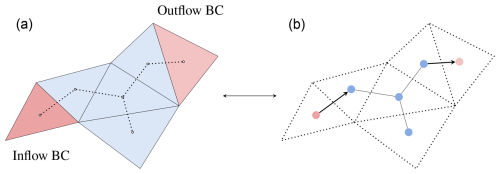
Figure 3 Schematic representation of an arbitrary triangular volume mesh (a) with two ghost cells for inflow and outflow boundary conditions (BCs). The ghost cells (red) are added in correspondence to a boundary cell which receives a given boundary condition. In the dual graph (b), a directed edge is added from the ghost cell to the domain cell or vice versa, depending on whether the boundary condition is an inflow or an outflow, respectively.

2.4 Rotation-invariant inputs

Most deep learning models consider coordinate-dependent features, such as the x and y components of the slopes. When applying a rotation to a domain, these values change, causing a change in the output, which is not necessarily equivalent to the applied rotation. This is a well-studied challenge in deep learning (DL) models (Bronstein et al., 2021) and can be solved via data augmentation, i.e. by training the model using rotated instances of the training data, or by modifying the deep learning model (e.g. Lino et al., 2022). Since the outputs of our model are scalars, we avoid using any rotation-dependent features to simplify the model and obtain a rotation-invariant model; i.e. rotations of the inputs do not affect the output. The static node features can then be expressed as ${\mathit{x}}_{\mathrm{si}}=(a_i,e_i,m_i,w_i^t)$, where a_i is the area of the ith finite-volume cell, e_i its elevation, m_i its Manning coefficient, and $w_i^t$ its water level given by the sum of the elevation and water depth at time t. To determine the values of elevation e_i,m, Manning coefficient m_i,m, and water level $w_{i,m}^t$ at the coarser scales, we perform a mean pooling operation from the finest scale to each of the coarser scales as in Eq. (5). As edge features, we consider ε_ij=(l_ij), where l_ij is the length of the dual edge between node i and node j. The dynamic node features are defined as x_di = ${\mathit{u}}_i^{t-p:t}$ = (${\mathit{u}}_i^{t-p}$, …, ${\mathit{u}}_i^{t-\mathrm{1}}$, ${\mathit{u}}_i^t$), with ${\mathit{u}}_i^t$ = ($h_i^t$, $|q{|}_i^t$), where $h_i^t$ is the water depth at time t and node i and $|q{|}_i^t$ is the unit discharge at time t and node i.

2.5 Loss function

We employ a multi-step-ahead forecasting loss ℒ_f that considers multiple model outputs using its own predictions as inputs. This helps the model deal with incorrect inputs and is useful in reducing the accumulation of errors in time (Bentivoglio et al., 2023). It can be expressed as

$$\begin{array}{}\text{(9)}& {\mathcal{L}}_f={\displaystyle \frac{\mathrm{1}}{HO}}\sum _{\mathit{\tau }=\mathrm{1}}^H\sum _{o=\mathrm{1}}^O{\mathit{\gamma }}_o|{\widehat{\mathit{u}}}_o^{t+\mathit{\tau }}-{\mathit{u}}_o^{t+\mathit{\tau }}{|}_{\mathrm{2}},\end{array}$$

where ${\mathit{u}}_o^{t+\mathit{\tau }}\in {\mathbb{R}}^N$ denotes the predicted hydraulic variables at time t+τ, H is the prediction horizon, O is the number of output hydraulic variables, and γ_o denotes coefficients used to weigh the influence of each hydraulic variable on the loss.

3 Experimental setup

3.1 Synthetic dataset

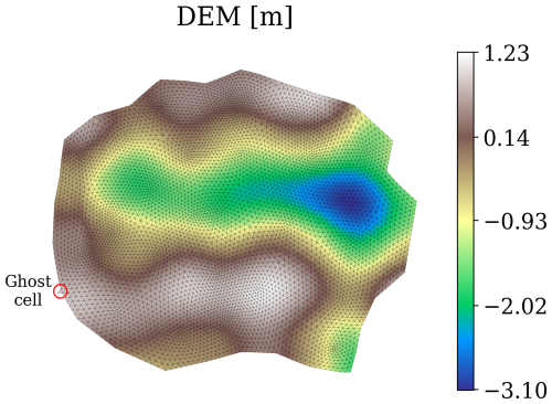
We created a synthetic dataset of dike-breach flood simulations using the numerical software Delft3D (Deltares, 2022). Each simulation is discretized via an irregular mesh created from randomly generated polygons, based on ellipsoidal shapes, as described in Sect. 2.1. The multi-scale mesh obtained with this procedure has a total of four scales. This is an arbitrary choice selected to showcase the expressivity of the model, but a different number of mesh scales would work as well, unless the coarsest scale has excessively few cells. For each mesh, we use a randomly generated digital elevation model (DEM) based on Perlin noise and combined with a small slope in a random direction, as exemplified in Fig. 4. As a boundary condition, we apply an inflow discharge hydrograph to one random border edge. The hydrograph's shape is generated based on Weibull-like probability density functions with different shape parameters (Bhunya et al., 2011). All hydrographs are right-tailed since most dike-breach hydrographs have this shape (e.g. D'Oria et al., 2022; Shustikova et al., 2020), and their peaks vary from 150 to 300 m³ s⁻¹, as shown in Fig. 6, in line with realistic breach inflows. For Manning's roughness coefficient, we used a spatially uniform value of 0.023 m${}^{-\mathrm{1}/\mathrm{3}}$ s, which is kept the same throughout all simulations. The dataset comprises 100 simulations, 60 used for training, 20 for validation, and 20 for testing. Each simulation has as output a temporal resolution of 2 h for a total simulation time of 96 h, or 48 steps ahead. The datasets' statistics in terms of elevation (above sea level), number of cells, cell area, edge length, and total flood volume are reported in Table 1. Compared to the dataset in Bentivoglio et al. (2023), this has more complexity, in terms of both mesh structure and discharge conditions.

Table 1 Mean and standard deviation of elevation (above sea level), number of cells, cell area, edge length, and total flood volume for the training, validation, and testing datasets. All geometric variables refer to the properties of the finest mesh in each dataset.

Figure 4 Example mesh with the corresponding digital elevation model (DEM) for one simulation in the synthetic dataset.

3.2 Case study: dike ring 15

We assess the transferability of the trained model by applying it to dike ring 15 Lopiker- and Krimpenerwaard in the Netherlands, which surrounds and protects the area between Rotterdam and Utrecht (Fig. 5). This area is prone to flooding and protected entirely by a system of levees. This case study has an area of 31 400 ha, with a total population of 201 500 inhabitants and an expected flood damage cost per event of EUR 5.1 billion (Boon and Witteveen+Bos, 2011). We chose this area because, depending on the location of the breach, the basin has a bathtub or sloped response, meaning that water fills up the domain evenly or has a preferential drainage direction, respectively (Rijkswaterstaat, 2014). We simplified the hydraulic components not represented in the training dataset. Specifically, we removed all waterbodies and every infrastructure that is not directly included in the DEM. Moreover, we assumed constant roughness coefficients throughout the whole area.

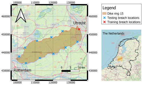
Figure 5 Dike ring 15 in the Netherlands (coordinate system EPSG:28992 Amersfoort / RD New). The crosses indicate the location of the dike breaches used for training and testing. The maps are taken from ©OpenStreetMap contributors 2024. Distributed under the Open Data Commons Open Database License (ODbL) v1.0.

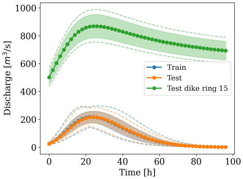
Figure 6 Distribution and shape of the hydrographs used as inputs for the training (blue), synthetic test (orange), and dike ring 15 test (green) simulations. The shaded region indicates 1 standard deviation away from the mean at each time step. The dashed lines represent the envelopes of the minimum and maximum discharges at each time step.

As boundary conditions, we created a set of inflow discharges that follow a different distribution from the training ones. This has an initial rise, following a hypothetical widening of the breach, and a decreasing limb in time that ends with non-zero discharge. We also increased the peak discharge to match realistic values for the case study considered, with values between 700 and 1000 m³ s⁻¹, corresponding to inflows of a fully developed breach, which could be more than 100 m wide. This results in an approximately 9-fold increase in the total flood volumes with respect to the synthetic dataset. For the breaching locations, we selected 11 approximately equidistant spots along the contour of the dike ring (see Fig. 5). This allows us to capture the comprehensive hydraulic responses of the basin.

The selected case study is more than twice as big as the synthetic datasets and has different elevation patterns, leaving more space to develop different flood dynamics. Hence, we decided to also test the model with a fine-tuning step, employing a single simulation for training and validation. In the experiments, we analyse the effect of adding this fine-tuning step after training the model on the synthetic dataset.

3.3 Normalization

The static attributes (node and edge features) are determined at all scales when creating the dataset. Since the values of areas a and edge lengths l change significantly across scales, we standardize those features separately for each scale. Specifically, we collect all training instances of a given variable x at mesh scale ℳ_m and determine their mean μ and variance σ. The normalized variables are then obtained as $\widehat{x}=\frac{x-\mathit{\mu }}{\mathit{\sigma }}$, where $\widehat{x}$ indicates the standardized variable. The remaining variables are not processed by any normalization procedure.

3.4 Training setup

We trained all models with the PyTorch (Version 2.0.1) (Paszke et al., 2019) and PyTorch Geometric (Version 2.4) (Fey and Lenssen, 2019) libraries, using the Adam optimization algorithm (Kingma and Ba, 2014). We performed several preliminary trials to identify a set of suitable training hyperparameters for the experiments; see Table D1. We used a learning rate scheduler with a fixed step decay of 0.7, every 20 epochs, starting from 0.003. The training was carried out for 200 epochs with early stopping, using 16-bit mixed precision to decrease the computational burden. During training, we clipped the gradients with a value higher than 1 to improve training stability and employed a curriculum learning strategy as in Bentivoglio et al. (2023), with a maximum training prediction horizon H=6 steps ahead (Eq. 9). We used p=2 previous time steps as dynamic inputs; i.e. ${\mathbf{X}}_d=({\mathbf{U}}^{t-\mathrm{2}},{\mathbf{U}}^{t-\mathrm{1}},{\mathbf{U}}^t)$. The coefficients used in the loss function (Eq. 9) are γ₁=1 for the weight of the water depths and γ₂=7 for the weight of the unit discharge. We used these values to weight more water depths, whose values are generally more than 10 times larger than the discharge ones, as we deem them more important.

In terms of hardware, we employed an NVIDIA A100 80 GB PCIe (Delft High Performance Computing Centre, 2022) for training and deployment of the deep learning models and an Intel^® Core™ i7-8665U at 1.9 GHz CPU for the execution of the numerical model. Note that the numerical model cannot run on GPUs, but we used the available OpenMP option to parallelize the computations on eight CPU threads.

3.5 Metrics

We evaluated the models' performance using a multi-step-ahead mean absolute error (MAE) for each hydraulic variable ${\widehat{\mathit{u}}}_o^{\mathit{\tau }}$ over the full simulation, expressed as

$$\begin{array}{}\text{(10)}& {\mathrm{MAE}}_o={\displaystyle \frac{\mathrm{1}}{H}}\sum _{\mathit{\tau }=\mathrm{1}}^H|{\widehat{\mathit{u}}}_o^{\mathit{\tau }}-{\mathit{u}}_o^{\mathit{\tau }}{|}_{\mathrm{1}},\end{array}$$

with H being the prediction horizon. Note that while the training loss in Eq. (9) is evaluated over a limited number of time steps, the validation loss function in Eq. (10) is evaluated on the full simulation to mimic the testing conditions.

We also measured the spatio-temporal error distribution of the water depth using the critical success index (CSI) for threshold values of 0.05 and 0.3 m as in Bentivoglio et al. (2023). The CSI measures the spatial accuracy of detecting a certain class (e.g. flood or no-flood), and for a given threshold it is evaluated as

$$\begin{array}{}\text{(11)}& \mathrm{CSI}={\displaystyle \frac{\mathrm{TP}}{\mathrm{TP}+\mathrm{FP}+\mathrm{FN}}},\end{array}$$

where TP denotes the true positives, i.e. the number of cells where both numerical and deep learning models predict water depth above a given threshold; FP denotes the false positives, i.e. the number of cells where the deep learning model wrongly predicts water depth above a given threshold; and FN denotes the false negatives, i.e. the number of cells where the deep learning model does not predict water depth above a given threshold. We measured the computational speed-up as the ratio between the computational time required by the numerical model and the inference time of the deep learning model. We did not consider the computational time to create the meshes, since they are needed for both methods. Unless otherwise mentioned, the deep learning model is run in parallel over all testing simulations, differently from the numerical model (see Appendix C). This choice is reasonable since we can use this model for probabilistic forecasts, where multiple simulations may be run in parallel.

4 Results

4.1 Comparison with SWE-GNN

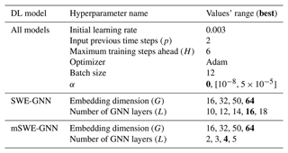
To highlight the improvements given by multi-scale modelling, we compared the mSWE-GNN model with an enhanced SWE-GNN model that includes ghost cells, rotation-invariant inputs, and the 1D CNN in the decoder but lacks the multi-scale component. We did not compare it with the standard SWE-GNN since it would not be able to run without a numerical input. We also did not compare it against other baselines as the SWE-GNN performs better than them (Bentivoglio et al., 2023), so we assumed the same holds for the enhanced version. Both models underwent a hyperparameter search procedure based on the number of GNN layers and the number of hidden features, as reported in Table D1.

This resulted in a set of models with different performance levels in terms of accuracy and speed, as reported in Fig. 7. The results show that the multi-scale structure helps the model to better capture flow variations across time, resulting in a better Pareto front for validation losses and CSI. The mSWE-GNN has, on average, more parameters than the SWE-GNN because it has several GNNs (two per scale, except one for the bottleneck), which makes it by default bigger. Despite this, the mSWE-GNN is comparatively fast, with speed-ups of up to 1200 times, since at the finest scale it has fewer layers than the SWE-GNN. This substantially reduces the computations since the finest scale is the one with the most nodes and edges. Moreover, the training process also resulted in being more stable in the mSWE-GNN, probably due to the lower number of GNN layers.

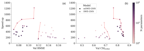
Figure 7 Pareto front of the mSWE-GNN and SWE-GNN models for speed-ups: validation RMSE (a) and validation CSI with a 0.05 m water depth threshold (b). The models' size varies with the number of hidden features and number of GNN layers.

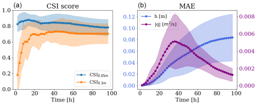
For the remaining analyses, we selected the mSWE-GNN model with the best performance, which consists of four GNN layers for each scale, a hidden feature dimension of 64, and around 811 000 learnable parameters. Despite the limited number of training samples and the amount of variability in simulated conditions, the model captures the flow patterns. Figure 8 reports the evolution of the critical success index (CSI) for the water depth thresholds of 0.05 and 0.3 m and the mean absolute errors (MAE) for water depth and unit discharge for the test dataset. CSI_0.05 m stays constantly high for all simulations. On the other hand, CSI_0.3 m starts low; this is due to an initial scarcity of water depths higher than 0.3 m, which skews the performance to lower values. The MAE of unit discharge seems correlated with the input breach discharge values, meaning that the biggest errors occur at the hydrograph peak and the smallest close to the tail. Indeed, the highest errors are generally located near the breach location, where the most rapid processes occur. Thus, when the inflow discharge decreases, so does the error. The MAE of water depth instead rises with time, as also reported in Bentivoglio et al. (2023). The main reason for the increase in water depth MAE over time is that as the flood progresses, it covers a greater spatial extent, increasing the number of cells where prediction errors can occur. In this case, however, the errors plateau at the end of the inflow hydrograph, indicating that water flow is stopping.

Figure 8 Temporal evolution of CSI scores (a) and MAE of water depth h and unit discharge q (b) for the test dataset. The confidence bands refer to 1 standard deviation from the mean.

4.2 Transfer learning to realistic case study

After training the model with the synthetic dataset, we tested it on dike ring 15 for different breach locations with varying discharges. The zero-shot testing of the model without any fine-tuning resulted in modest performance levels, seen in Table 2. We attribute this mismatch to not only the difference in total flood volume but also the domain size and the different elevation patterns when compared to the training ones (see Table 1). Moreover, this implies different hydraulic dynamics, such as the presence of a sloped basin which accumulates water in a downstream area (in the bottom left of the domain) without further propagation, which are not sufficiently represented in the training domain.

Table 2 Effect of fine-tuning the mSWE-GNN model on dike ring 15. The provided uncertainty estimates account for the variability across different simulations. All metrics refer only to the finest mesh.

We then performed a fine-tuning step consisting of training the previously trained model again with one extra simulation from the new case study. We trained and validated data on the same simulation since we wanted to minimize the number of data needed to fine-tune the model. While in principle this might lead to overfitting, this was not the case here. This is probably due to the inductive biases of the model which constrain the model to learning only local dynamics. Additionally, the training process considers only a limited number of predicted steps ahead, while the full simulation has many more. Consequently, the model is forced to learn different dynamics in time rather than overfitting on a single temporal pattern, even if we are training on a single simulation. Table 2 shows that adding just one simulation improves the testing performance on the rest of the dike ring by 158 % and 62 % in terms of MAE for water depth and discharge, respectively, and by 38 % and 78 % for CSI_0.05 m and CSI_0.3 m.

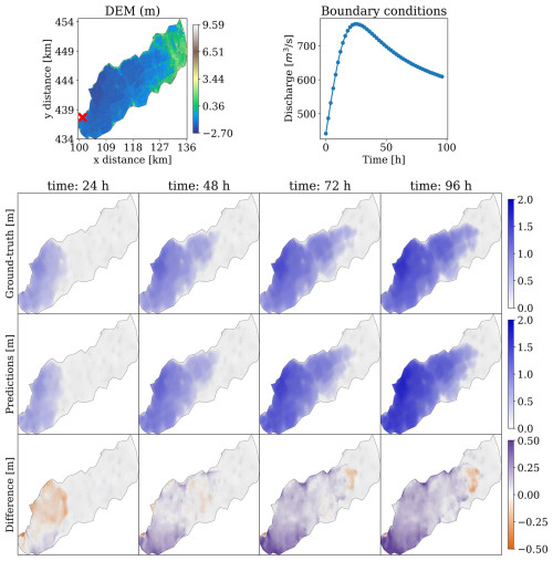
Figure 9 The mSWE-GNN's predictions for water depth on a testing simulation for dike ring 15. The topography is presented in the top-left plot and the discharge hydrograph in the top right. Below is the evolution over time for the ground-truth output of the numerical simulation (top row) with the predictions (middle row). The difference (bottom row) is evaluated as the predicted value minus the ground-truth one; thus, positive values correspond to model over-predictions, while negative values correspond to under-predictions. All plots represent values only on the finest mesh.

Figure 9 shows the model performance for the prediction in time of water depth for one test case. Water depths are predicted well overall in the domain, including water accumulation in the western part of the area. While the absolute values of the difference may be relatively high in these areas, they do not matter as much for practical purposes since those locations are flooded with a high water depth either way; thus the associated damage will be equivalent.

Figure 10 shows that the spatio-temporal evolution of the predicted flood is in line with the corresponding numerical simulations, as indicated by the low errors in flood arrival times (FATs) for the critical threshold of 0.05 m of water depth. FATs indicate the arrival time of water with a given depth threshold for each cell in the domain. Most errors are located at the wave front during the end of the simulation, as previously mentioned, or in false-positive areas that are not flooded in the numerical model.

Figure 10 Flood arrival times (FATs) for a water depth threshold of 0.05 m for a test case from dike ring 15, given for the numerical simulation (a), the predictions (b), and the difference (c). Darker colours in the first two maps indicate a faster arrival of the water, while white cells indicate absence of water. In the difference map, positive values indicate that the model estimates later arrival times than the numerical simulation, while negative values indicate that the model predicts earlier arrival times. All plots represent values only on the finest mesh.

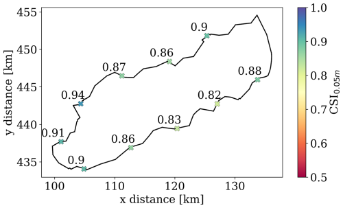
Figure 11 Performance in terms of CSI for a water depth of 0.05 m for all testing breach locations in dike ring 15 for the fine-tuned mSWE-GNN.

Figure 11 indicates that the model performance is consistently high for all testing breach locations of the dike ring 15 dataset, as suggested by the high CSI_0.05 m values, which are always above 0.8. One reason why the model performs so well is that the final flood map tends to converge to the downslope accumulation area in the bottom-left area of the domain. This also proves that the model can correctly model the response dynamics of the system, independently of where the breaching starts.

The good performance of the mSWE-GNN model is accompanied by a substantial speed-up of the underlying model. When testing, the model has a speed-up of more than 700 times with respect to the original simulations, as highlighted in Table A1. This indicates a good scaling with the size of the domain, with higher speed-ups for bigger domains. One other possible explanation is related to the simulated discharges. Numerical simulations of slow flows are generally more stable and faster to compute than those with high Froude numbers, which are more present in dike ring 15. Contrarily to numerical models, the mSWE-GNN has no such stability constraints, which makes it unbound by the same limitations and thus faster.

4.3 Ablation study

Finally, we performed an ablation study to determine the role of the different components in the mSWE-GNN (Table 3), such as the multi-scale module, the convolutional decoder, and the rotation-invariant inputs. We also reported the performance of the best SWE-GNN model from Sect. 4.1. The results reported in Table 3 show that all of the added or removed components contribute to the performance on the test dataset. The speed-up was consistent throughout all mSWE-GNN configurations, and we report it in Table A1.

Table 3 Ablation study on the removal or addition of individual architectural and training components for the synthetic testing dataset. These are using a learnable pooling for the downsampling operator, removing skip connections in Eq. (7), removing the 1D CNN in Eq. (8), and using rotation-dependent inputs. The best results are reported in bold; w/o denotes “without”.

4.3.1 Multi-scale module

We analysed the effects of using a learnable downsampling operator in place of a mean pooling operator in Eq. (5) and of removing skip connections in Eq. (7). For the learnable downsampling operator, we used a three-layer MLP shared across each intra-scale edge that takes as inputs the dynamic node feature at nodes i in ℳ_m and node j in ℳ_m+1, similarly to Eq. (6).

Using a learned downsampling operator results in a lower performance. We argue this is caused by the unnecessary complexity of the operation and by the common mean aggregation term, which is needed to make the model work with a flexible number of nodes and cancels out the expressivity of the MLP.

Removing skip connections does not influence the performance as much. This indicates that most of the computations are performed after the architecture bottleneck, while the down-going branch is responsible for smaller details that are not captured in the up-going branch. This means that the number of layers in the down-going branch can probably be reduced while keeping good performance with less model complexity.

4.3.2 Decoder

We compared the convolutional decoder (Eq. 8) with a residual connection which simply sums the output of the previous time step and the output of the decoder's MLP before applying a ReLU activation; i.e. ${\widehat{\mathbf{U}}}^{t+\mathrm{1}}=\mathit{\sigma }\left({\mathbf{U}}^t+\mathit{\phi }\left({\mathbf{H}}_d^{\left(L\right)}\right)\right)$. Using the 1D CNN in the decoder results in better testing and validation metrics, meaning that different time steps contribute unevenly to the final model output. This allows the model to better capture variations in time, especially due to rapid variations in boundary conditions.

4.3.3 Rotation-invariant inputs

We added the x and y components of the slope and orientation of mesh edges as static inputs to show that including rotation-dependent inputs worsens generalization (Table 3). The reason for this is that all simulations are quite different from one another in terms of breach location and orientation of the meshes. Consequently, a model with rotation-dependent inputs would require far more training data to generalize well to all spatial configurations.

5 Discussion

We proposed a multi-scale graph neural network model (mSWE-GNN) that can generalize flood simulations to unseen irregular meshes, topographies, and time-varying boundary conditions, with speed-ups up to 700 times compared to the underlying numerical model. The mSWE-GNN generalizes well to realistic case studies with as little as one fine-tuning simulation. We expect the model to further improve performance and reduce risk of overfitting by increasing the number of fine-tuning simulations. This result is in line with a similar finding for pluvial flooding, where one fine-tuning simulation was enough to help in generalization to diverse case studies (Cache et al., 2024). Since the model can generalize well with as few as 60 training simulations, we believe that training the model on a substantially larger number of data might even remove the need for fine-tuning, although this could still be needed for more complex domains.

One key to the model's success comprises the different scales, which enable learning varying speeds of flood propagation and capturing the hydraulic processes, contrarily to the SWE-GNN, which learns a more limited range of speeds. The multi-scale nature of the model allows optimizing computations for areas where fine details are relevant only in small portions of the domain. In the same way, scales can be used to better include the presence of 1D structures in the domain such as channels and elevated elements. These can be included in the coarser meshes using slimmer cells that overlap with the channel, as done in numerical models (Bomers et al., 2019). On the other hand, structures that markedly influence the flow propagation, like levees, can simply be omitted in the coarser meshes by leaving holes in correspondence to them. This artificially blocks the possibly faster flow propagation of coarser scales. Once over-topping of said levee occurs at the fine scale, then the faster propagation can begin anew at the coarser scales. We improved the model generalization to unseen meshes by considering rotation-invariant inputs. This was possible because we considered scalar outputs, since we deemed the intensity of the flood more important than also knowing its direction for practical uses (Kreibich et al., 2009).

While the current model framework can work for dike-breach floods, we did not evaluate it for other types of floods. For river and coastal floods, the model should work without any changes since the inputs are of the same type as dike-breach floods, e.g. upstream discharge hydrographs or seawater levels. On the other hand, pluvial floods require precipitation as a further input. Assuming rainfall as a spatially distributed variable, it could be added as a dynamic forcing; this could work in a way similar to how it works for static features but changing at each time step, independently of the predicted output. For urban floods, the drainage system should also be included. This could be done, as in numerical methods, by coupling the overland flow, predicted by the mSWE-GNN, with a 1D model for the sewers, possibly with another learned GNN as in Garzón et al. (2024).

Regarding the process of mesh creation, we constructed the coarse-scale meshes based on the boundary polygon of the areas considered. However, this requires the user to create a mesh with a top-down approach and limits the use of an existing fine-scale mesh. This could be solved using a different multi-scale mesh creation approach. For example, Lino et al. (2022) used a sampling strategy based on regular partitioning of the domain, which allows the coarse meshes to have similar edge lengths, independently from the fine mesh. Alternatively, we could use the same mesh creation procedure to only generate the coarse-scale meshes and use existing detailed meshes on the fine scale. The latter may be problematic when fine structures are present that markedly alter the flow of the flood, making the automatic mesh generation procedure challenging.

The boundary condition insertion also technically works for given water levels at the boundary, but we did not analyse it. Moreover, we did not analyse the performance for multiple concurring boundary conditions, despite the model already being able to accommodate them. We employed a constant and spatially uniform roughness coefficient, meaning that we did not assess how the model generalizes to different values and spatial distributions. This might lead to different dynamics that, following the same reasoning as for the different speeds of propagation, the model should still be able to capture.

To simplify the hyperparameter selection process, we also selected an equal number of GNN layers for all scales. Instead, we could further optimize the Pareto front by changing the number of layers at each scale independently. Additionally, we did not make a comparison with other recent developments in deep learning models, such as Fourier neural operators (Li et al., 2020) or neural fields (Yin et al., 2023), since either they do not generalize across different irregular meshes or their application to flooding would not be trivial. We remark that most of the speed-ups come from the use of a GPU, as all processes are parallelizable. This is a well-known benefit of deep learning models, and the mSWE-GNN enjoys it.

For practical applications, there are still several components that must be included to match numerical models for real case studies. Future studies should investigate the inclusion of time-varying breach growth models or components such as existing waterbodies and linear elements, such as roads and secondary dikes. Eventually, the proposed model could be used to create a probabilistic framework to assess many different flood scenarios and uncertainties in boundary conditions, breaching conditions, and topography (Vorogushyn et al., 2010).

6 Conclusion

We proposed a multi-scale hydraulic graph neural network, called the mSWE-GNN, that models flood propagation in space and time across multiple resolutions. As input the model takes static attributes, such as topography, and dynamic attributes, such as water depth and unit discharge at time t, and predicts their evolution at the following time step t+1. This is done via a U-shaped architecture that applies graph neural networks at different scales and combines them with downsampling and upsampling operators. This captures a broader range of dynamics by jointly modelling the flood propagation speeds at different scales. We included time-varying boundary conditions via ghost cells. We also improved the generalization to unseen meshes by using rotation-independent inputs.

The model can accurately replicate the overall dynamics of the flood evolution over unseen meshes, topographies, and boundary conditions, with no dependence on any numerical solver. The model can also generalize to realistic case studies with more complex and bigger domains than the training ones with only a single fine-tuning simulation. Moreover, the new model is better and faster than its non-multi-scale counterpart, indicating that the insertion of this module contributes significantly to the model's performance.

Overall, these results open up new possibilities for modelling flood uncertainties probabilistically in real case studies. This will allow practitioners to have a complementary tool for the fast evaluation of several flooding scenarios before analysing in more depth critical ones with numerical models.

Appendix A: Additional results

We analysed the evolution in space and time of the unit discharges for one test simulation in the synthetic dataset to highlight that the model is now able to correctly model the filling and emptying dynamics. Figure A1 shows that discharges are modelled very well by the model, in both the ascending and the descending phases of the input hydrograph. This is in line with the hypothesis of Bentivoglio et al. (2023) according to which the model is able to capture this draining and the decreases in discharges when presented with sufficient samples of it in the training dataset.

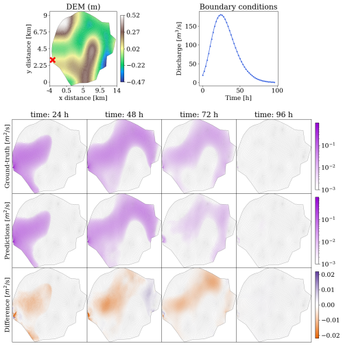
Figure A1 The mSWE-GNN's predictions for unit discharges in a test simulation from the synthetic dataset. The evolution over time for ground-truth output of the numerical simulation (top row) with the predictions (middle row) is represented using a logarithmic scale to better appreciate the values' distribution. The difference (bottom row) is evaluated as the predicted value minus the ground-truth one and is kept with a standard scale to highlight the use of the logarithmic scale; positive values correspond to model over-predictions, while negative values correspond to under-predictions.

We report the execution runtimes of the numerical and trained mSWE-GNN models for both testing datasets. Since the deep learning model is run in parallel, the prediction times per simulation are averaged out through all simulations. We measure the runtime variability by running the model 10 times and reporting the corresponding mean and standard deviation. For both dataset, the model achieves a great speed-up, of more than 2 orders of magnitude, which could further increase when selecting a smaller model from the Pareto front in Fig. 7.

Table A1 Runtimes of the numerical model and the selected mSWE-GNN model for the two testing datasets and their respective speed-ups.

In terms of training times, the SWE-GNN model took between 5 and 30 h, while the mSWE-GNN took between 2 and 15 h, depending on the model complexity. The fine-tuning process, with the selected mSWE-GNN model in Sect. 4.1, took around 20 min. The fine-tuning time can be reduced to 5 min by decreasing the number of epochs while still obtaining comparable performance. If we evaluate the speed-up on dike ring 15 also including the time to run the fine-tuning numerical simulation and the time to train it, we still achieve a speed-up of 4 to 8 times, depending on the number of fine-tuning epochs.

Figure A2 Performance in terms of validation loss and CSI_0.05 m for varying values of the mass conservation weight α_M.

Appendix B: Mass conservation

We proposed a regularization term ℒ_c that enforces a global mass conservation per each time step. This reads as

$$\begin{array}{}\text{(B1)}& {\mathcal{L}}_c=\left|\sum _{i=\mathrm{1}}^N{a}_i\mathrm{\Delta }{\widehat{h}}_i-Q\mathrm{\Delta }t\right|,\end{array}$$

where N is the number of nodes in the output mesh; $\mathrm{\Delta }{\widehat{h}}_i$ is the variation in predicted water depth at node i; $a_i\mathrm{\Delta }{\widehat{h}}_i$ is the variation in predicted volume at node i; Q is the inflow discharge; and Δt is the time interval between t and t+1, in which the discharge is assumed to be constant. This enforces the total amount of volume entering the domain QΔt to be redistributed in the domain so that the volume is conserved.

We carried out supplementary experiments to explore the benefit of adding this term to the forecasting loss in Eq. (9). The combined loss ℒ can be expressed as

$$\begin{array}{}\text{(B2)}& \mathcal{L}={\mathcal{L}}_f+\mathit{\alpha }\cdot {\mathcal{L}}_c,\end{array}$$

where α weighs the contribution of the mass conservation term.

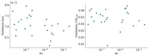
Figure A2 shows that the validation loss and CSI are slightly negatively correlated with α, meaning that losses tend to improve and classification worsens. The reason why losses slightly improve might be because the added loss term depends only on the predicted water depth, so it forces that value to be more precise. However, the conservation loss acts globally for each time step instead of locally. Therefore, the model cannot correctly improve the spreading of the flood but only the absolute values of total water depth. From these plots, we cannot extract any meaningful conclusion since there is no statistical significance, as highlighted by p values of 0.42 and 0.48, respectively. Moreover, the performance in the testing dataset follows an opposite trend, further indicating that inclusion of this term is not consistently better.

This in part contradicts the idea of physics-informed neural networks (PINNs), according to which adding a physical loss term improves performance (Raissi et al., 2019). One motivation is that the loss we employ does not rely on auto-differentiation in the same way that PINNs do. We also evaluate it globally, rather than at individual points as in PINNs. Implementing a PINN loss would require adjustments to the model's inputs and outputs to allow auto-differentiation to estimate the derivatives of the predicted target variables. Moreover, PINNs are typically designed to solve a given physical problem for a single set of boundary and initial conditions, thus limiting the model's capacity to generalize across varying conditions, which is a prerogative of our work. Although we did not adopt this approach here, it could be explored in future studies. Notably, our loss term is independent of ground-truth data, making it a possible self-supervised loss that could be explored in future works.

Appendix C: Parallel simulations

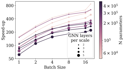
We refactored the code to compute all testing simulations in parallel, instead of in series, using batches. To analyse the speed-ups provided by parallel execution, we selected all models in the Pareto front of the mSWE-GNN in Fig. 7, which have different numbers of parameters and numbers of GNN layers per scale. We then ran the models using an increasing number of simulations in parallel, indicated by the batch size.

Figure C1 indicates that the speed-up almost doubles with the batch size, independently of the size of the model. It also highlights that the main computational effort comes from an increase in the number of GNN layers, rather than just the total number of model parameters, as also reported in Bentivoglio et al. (2023). When running 20 simulations, i.e. the full testing dataset, in parallel instead of in series, we provide a further speed-up of 4.5 times on average across different model sizes. Further speed-ups may be achievable by optimizing the code; for example just-in-time (JIT) compiling of the PyTorch code into optimized kernels can further accelerate the execution of the model by 2 or 3 times (Paszke et al., 2019). In a similar fashion, intelligence processing units (IPUs), which are novel processing units that perform faster inference on graphs, can further speed up the model by 2 to 4 times (Knowles, 2021).

Figure C1 Speed-ups of the mSWE-GNN for the synthetic test dataset, considering varying batch sizes, i.e. how many simulations are run in parallel. The results are reported for all Pareto front models from Fig. 7. Both axes are on a log₂ scale.

Appendix D: Hyperparameter ranges

We reported the hyperparameters used to create and train the model and their ranges in Table D1. Since the number of hyperparameters is high, some values are taken based on similar studies in the literature (e.g. Bentivoglio et al., 2023). For the mass conservation weight α in Eq. (B1), we uniformly sampled values in an interval from 10⁻⁸ to $\mathrm{5}\times {\mathrm{10}}^{-\mathrm{5}}$ using a logarithmic distribution. The reason why these values are small is due to the flood volumes being more than 10⁶ times higher than water depths.

Table D1 Summary of the hyperparameters and related values' ranges employed for the different deep learning models. The bold values indicate the best configuration in terms of validation loss.