An efficient method to simulate wildfire propagation using irregular grids

Climate change and land use changes are projected to make wildfires more frequent and intense, with a global increase in the number of extreme fires of up to 14 % by 2030, 27 % by the end of 2050, and 57 % by the end of the century (United Nations Environment Programme & GRID-Arendal, 2022). These values were forecasted by a Representative Concentration Pathway with a radiative forcing value of 6 W m⁻², which represents the energy imbalance in Earth's energy system caused by greenhouse gases and other factors, in the year 2100. This latest information has increased interest regarding how large-scale, often catastrophic, events can be reduced and more effectively managed. One critical area revolves around real-time fire line prediction and how resources can be better deployed to reduce the propagation of wildfires. In this paper a novel software platform called the Irregular Grid Software (IGS) was developed, which allows for the simulation of wildfires on a configurable grid using mathematical models for fire propagation. The aim of the IGS was to explore computational differences between different grid types and a comparison to preexisting software while producing outputs of an acceptable similarity to that preexisting software. The configurable grid was built using a Voronoi diagram, where a fire can spread between polygons, propagating throughout the grid. The configurable grid allows for cross comparison of both regular grids, such as square, hexagonal, and triangular, and irregular grids, such as a randomly seeded Voronoi diagram and a newly developed flammable resolution grid (FRG). The FRG was adapted to focus attention on areas of higher importance, which provides greater precision at the cost of extra computing time. The irregular grid approach and ForeFire, an existing industry-standard program, were compared. The comparison included simulations of wildfires located in the Wicklow Mountains, in Ireland, a region used by fire services for exercises. The performance of the grid-based techniques was examined using a set of experiments to characterise the model's response to key factors such as wind, elevation, and fuel type. The objective of this paper was to compare the various grid types on the metrics of similarity with ForeFire and computational time while also comparing the FRG to ForeFire on the same metrics with multiple sample wildfires. From the sample wildfires tested in this paper the results show that the IGS runs on average 34 times more quickly than ForeFire on the same computing platform while retaining an average result similarity of 80 % with ForeFire.

1 Introduction

All fires, including wildfires, require four components to support combustion (Helene et al., 2019). These are fuel (vegetation), an oxidising agent (oxygen in the air), heat (initiates the process), and a chemical chain reaction (to sustain combustion). Combustion is a chemical process in which fuel and an oxidiser combine to form heat greater than the fuel–oxygen mixture's flash point; if there is sufficient heat generated to overcome heat loss, combustion is sustained in a chain reaction. Together they make up the “fire tetrahedron”; a fire will cease to exist if any component is diminished within the tetrahedron (Fig. 1).

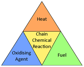
Figure 1 A 2D net of the fire tetrahedron, which shows all four components required to support combustion.

A wildfire is a potentially destructive fire that burns throughout an area; this includes forest fires and bushfires (Haghani et al., 2022). Usually, they begin in remote areas where there is a higher density of combustible vegetation such as grasslands and peatlands. They can sometimes threaten urban areas (Park et al., 2023). Wildfires can be caused by both natural events such as lightning and human-caused actions such as arson and farming techniques like slash-and-burn agriculture (Jiao et al., 2023; dos Reis et al., 2021). The frequency of wildfires has increased within forested extratropical and boreal regions in recent years; this is most likely due to climate change creating drier terrain, allowing for fires to burn more easily (Janssen et al., 2023; Abatzoglou et al., 2018; Halofsky et al., 2020). This however varies regionally, where factors such as the wildland–urban interface, land use changes, and fire exclusion policies can have an impact on the number of wildfires (Beltrán-Marcos et al., 2023; Piñol et al., 2005).

The devastation of wildfires can be measured in different ways such as fatalities, ecological damage, and economic damage. In California, USA, and Australia a small subset of wildfires that burn in terrain satisfying the correct conditions can potentially grow to be very large fast-burning fires, which can present an increased risk to life (Keeley and Syphard, 2021; Blanchi et al., 2014). Wildfires impact the ecosystem by destroying some of the flora and displacing or killing the fauna (Kala, 2023). When wildfires burn through terrain, they release carbon dioxide, further contributing to an increase in greenhouse gas emissions (Xue et al., 2024; Jones et al., 2019). The economic impact of wildfires includes damage to the agricultural and forestry sectors (Meier et al., 2023). When a wildfire spreads to an urban area, it can also cause considerable damage to town infrastructure (Park et al., 2023).

Countries that normally have a wet climate, such as Ireland, may also start to have an increased number of wildfires due to warmer temperatures, likely caused by climate change (McElwain and Sweeney, 2003; Boegelsack et al., 2018; Benyon et al., 2023). Wildfires have had an ecological impact in Ireland, where they tend to be smaller, slower-burning fires occurring mainly in bogs (peatlands), which are home to many rare species of both flora and fauna (Prat-Guitart et al., 2019). The high abundance of gorse (Ulex europaeus) in bogs makes them a common place for wildfires to occur as the plant is easily ignitable.

Even though wildfires that burn in Ireland, Australia, and the USA tend to have different burning behaviours, it is still possible to model them all as the underlying physics involved remain consistent. However, the parameters characterising fuel properties, terrain, and weather conditions need to be changed to represent the surrounding environment.

2 Overview of wildfire propagation models

With the increasing severity and frequency of wildfires in forested extratropical and boreal regions, the ability to model and predict wildfire propagation has become an invaluable asset to planners and firefighters (Penney et al., 2019). Planners can use this information to forecast and prevent fires, while firefighters can also use this information to find the optimal locations to apply interventions. These interventions include the construction of firebreaks, controlled burning, or the application of water using fire engines or helicopters equipped with a Bambi Bucket (SFI-Defence Organisation Innovation Challenge, 2024).

There are three main branches of wildfire modelling, which include statistical, empirical, and physical models (Weber, 1991). Statistical models are built on a statistical description of wildfires found by observing sample fires and are less focused on the thermodynamics of fire. The McArthur Forest Fire Danger Index is a statistical wildfire model (McArthur, 1966; Noble et al., 1980). The statical model was developed by only sampling fires burning dry grassland and forest litter, which means it needs to be used with caution on other fuel types. The model takes variables such as the temperature of curing for the fuel, air temperature, relative humidity, and wind velocity as input to produce a value representing the fire danger index. This value can then be converted into an estimated rate of spread for a wildfire.

Empirical models for wildfire spread are built upon the principles of the conservation of energy but do not differentiate between the various modes of head transfer. An empirical model was used to calculate fire spread through porous fuels in a fuel bed (Frandsen, 1971). This model calculates the rate of spread by finding the heat generated from the combustion of existing fuel and spreading this heat using the principles of the conservation of energy into the surrounding fuel until that fuel reaches its flash point and ignites.

Physical models do differentiate between the various modes of heat transfer and are deep-rooted in fundamental physics and the mathematics of combustion. A physical model was developed to find the rate of spread between two particles in a fuel bed (Fons, 1946). To calculate the rate of spread for the fire, this model found the time it took for fire to spread the distance from one particle to another. This method also used the principles of the conservation of energy, but this time it incorporated all three forms of heat transfer: conduction, convection, and approximating radiation.

One of the most cited wildfire models is the Rothermel model (Rothermel, 1972; Andrews, 2018). It was developed by Richard C. Rothermel in 1972 to help forest managers predict the behaviour of wildfires. The Rothermel model represents one approach to wildfire modelling as a physics-based, semi-empirical model formed using the conservation of energy that underpins many operational fire-modelling tools. The Rothermel model was based on the laws of heat transfer but was developed using experimental data from constructed fuel beds.

The Rothermel model takes multiple environmental, fuel, and fuel bed factors as input to produce an estimated rate of spread as an output Eq. (1). In the Rothermel model the numerator measures total heat transferred to neighbouring fuel, while the denominator measures energy required to ignite neighbouring fuel and R is the spread rate of the fire. It does this on a 1D line, but this can be expanded to more dimensions by measuring R on separate lines along each direction of interest. An easy way to interpret this is with a section of burning terrain acting as a heat source, while the fuel and fuel bed of the neighbouring terrain acts as a heat sink. If there is a surplus amount of heat produced to ignite the neighbouring terrain, the fire will spread (Fig. 2). The Rothermel model is normally presented using United States customary units. In this paper these values were converted into SI units within the fire simulations developed; this is the same as in ForeFire to simplify comparison in this paper. Another approach that could be considered would be to use the Rothermel equation reformulated in SI units (Wilson, 1980). The original Rothermel equation that was used in this paper is written as

$$\begin{array}{}\text{(1)}& R={\displaystyle \frac{I_{\mathrm{R}}\mathit{\xi }\left(\mathrm{1}+{\mathrm{\Phi }}_{\mathrm{w}}+{\mathrm{\Phi }}_{\mathrm{s}}\right)}{{\mathit{\rho }}_{\mathrm{b}}\mathit{\epsilon }{Q}_{\mathrm{ig}}}},\end{array}$$

where R ≥ 0 is the rate of spread in m s⁻¹ (ft min⁻¹), I_R ≥ 0 is the reaction intensity in J m⁻² s⁻¹ (Btu ft⁻² min⁻¹), 0 ≤ ξ ≤ 1 is the propagating flux ratio, Φ_w ≥ 0 is the wind factor, Φ_s ≥ 0 is the slope factor, ρ_b > 0 is the bulk density in kg m⁻³ (lb ft⁻³), ε > 0 is the effective heating number, and Q_ig > 0 is the heat of preignition in J kg⁻¹ (Btu lb⁻¹).

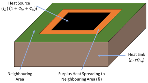
Figure 2 Example of how the Rothermel model functions, where the heat source is the location of the fire (where heat is being generated from combustion); the heat sink absorbs heat from the heat source, slowing down propagation; and the surplus heat is used to spread fire to the neighbouring area.

The Rothermel model is used as an optional fire propagation model in platforms such as Cell2Fire and ForeFire. There are three types of propagation models: cellular automata, cellular, and continuous. Cellular-automata models are restricted to a grid and a strict set of rules, where each cell is in a finite number of possible states and the state of one cell can influence the state of its neighbouring cells. Cellular models are also restricted to a grid, but the state of a cell is continuous and not confined to only influencing its neighbours (San Martin and Torres, 2023). Continuous models propagate over continuous space and therefore are not restricted to a grid or finite states.

Cell2Fire is a program that utilises cellular automata to simulate wildfire spread (Pais et al., 2021). Traditionally cellular automata have rules that express how the state of one cell interacts with its neighbouring cells. Cell2Fire can be given a fire spread model, a starting fire, and information about the environment to begin simulating fire spread. As Cell2Fire is a program built on cellular automata, it restricts the spread of fire to a regularly shaped square grid using the Moore neighbourhood, where each cell has eight neighbours (corner neighbouring cells inclusive) (Małecki, 2017). Cell2Fire generates the common ellipse shape of a wildfire for each cell based on the rate of spread. Once any point on the ellipse touches the centroid of a neighbouring cell, that cell will also begin generating its own ellipse to calculate the rate of spread. The uniform grid presents a trade-off between resolution and computation time. Low-resolution grids are fast but have the potential to be less precise. High-resolution grids are computationally intensive. This will be discussed in further detail later in the paper.

ForeFire is another program that simulates wildfire spread but does this over a continuous space instead of the discrete space used in cellular-automata models (Filippi et al., 2014). ForeFire uses a fire model, such as the Rothermel model, to compute propagation. It also takes spatial environmental data over a selected region of terrain as input. The environmental data contain wind data in the form of zonal (west-to-east) and meridian (south-to-north) wind speeds, elevation data regarding the terrain, and a numerical index representing different land cover types for the terrain. All data inputted into ForeFire are in the form of metric units. If the fire spread model required imperial or United States customary units (such as the Rothermel model), they need to be converted before calculating fire spread and converted back to metric units once fire spread has been calculated. ForeFire is seeded with information about the fire's starting location, the spatial resolution, and the duration of the simulation. During the simulation ForeFire calculates fire spread using the current fire location and environmental inputs. The increased fire spread perimeter is comprised of nodes called markers that ForeFire uses to continue spreading for the next iteration. Each marker has a propagation vector representing its movement direction and speed of propagation. The speed at which the marker moves at is determined by the fire spread model. If the distance between markers is greater than a selected spatial resolution, more markers will be created and redistributed along the fire front. If the distance between markers is less than a quarter of the spatial resolution, they will be merged into one marker (Fig. 3). For this paper the spatial resolution of ForeFire was set to the same as its default example's resolution of 30 m². On completion, the software returns the final set of coordinates (known as markers) describing the location of the fire front. The use of markers instead of a grid allows for increased resolution as their position is on a continuous plane, limited by the resolution of the input data and their set spatial resolution. However, the continual placing, removing, and moving of markers add extra computational burden on the simulation.

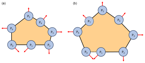
Figure 3 Example of ForeFire markers at time step 0 (a) and time step 1 (b). In this example the fire line (black line), markers (blue circles), the direction of spread for markers (red arrows), and where the fire has been (orange) are all shown. In panel (b) markers P₀ and P₁ will combine into one marker as the distance between them is a quarter of the spatial resolution. Marker P₇ will be created as the distance between markers P₅ and P₆ is greater than the spatial resolution.

The technique of simulating wildfires using the Rothermel model in this paper follows a similar methodology as was used to simulate wildfires using cellular automata (Zhang et al., 2021). In that paper wildfires progressed from a cell's centroid to neighbouring cell centroids at a rate determined by the Rothermel model. Once a wildfire had reached a neighbouring cell's centroid, that cell would also spread the wildfire to its neighbouring cells. Similar techniques will be used in the Methods section of this paper.

3 Methods

This paper's novel approach, named the Irregular Grid Software (IGS), was purposely designed to use the same input parameterisation as ForeFire to allow for a fair comparison between both platforms.

3.1 Resources

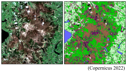
A satellite image of the region around Lough Dan, County Wicklow, Ireland, was used as input data for both ForeFire and the IGS. A random forest machine learning model was applied to the satellite data to produce a land cover map. Each pixel on the land cover map referenced an associated land cover type including pastures, sparsely vegetated areas, mixed forests, moors and heathland, urban fabric, waterbodies, clouds, and cloud shadows (Appendix A).

Each type of land cover was mapped to a set of physical attributes that were contained in a lookup table used by both programs. ForeFire contains one of these files called a fuel file, which was also used by default by the IGS (Fuels.ff Fuel Attribute Table, 2024). ForeFire's fuel file was indexed based on CORINE (Coordination of Information on the Environment) Land Cover classes (Copernicus, 2024). The fuel file contained values for fuel particle density (kg m⁻³), fuel particle moisture content, the ratio of fuel particle surface area to volume (m⁻¹), fuel height (m), the oven-dry fuel load (kg m⁻²), and fuel particle low heat content (J kg⁻¹) for the different land cover types. For both the IGS and ForeFire the Rothermel model had no mineral damping, and the moisture of extinction was set to 0.3 for all fuels. The listed fuel properties were required to run the Rothermel model. The land cover map had two additional fuel types for when it was not possible to identify the land type due to clouds or shadows. These fuel types were not present in the simulation area, as it was cloud free, so they did not affect either program.

The Sentinel-2 satellite data and a geographic information software, SNAP (Sentinel Application Platform) Desktop's elevation band generator, were used to produce an elevation map of the area (Copernicus Data Space Ecosystem, 2024; Science Toolbox Exploitation Platform, 2024). The elevation map gives the height in metres of elevation above sea level for each pixel in the satellite data.

For experimental simulation, a set of different wind speeds and directions were selected to allow for a comparison between ForeFire and the IGS under the same conditions. However, an API developed also allows for software such as Windy to provide live, forecasted, and historical wind data for simulations (Windy, 2024). Wind data were then split into zonal (west-to-east) and meridian (south-to-north) wind speeds which are mapped at each pixel across the satellite data.

ForeFire contained a tool that allowed for the land cover, elevation, wind data, and metadata to be combined into a single NetCDF file (Filippi et al., 2024b; Network Common Data Form (NetCDF), 2024). This same file was then used by both ForeFire and the IGS.

3.2 Simulating wildfire propagation using the IGS

The IGS was a Python program with the aim of generating a grid-based fire spread model that could be compared to ForeFire. The use of a static grid allows for a model to compute fire spread without having to continually move and add markers during the simulation as found in ForeFire.

A Voronoi diagram was used to create an irregular grid. They have been used to simulate the geographic spread of disease in the past (Hackett et al., 2021). A Voronoi diagram takes in a set of points called sites. From these sites edges (lines) are generated, equidistant between each pair of sites, perpendicular to the direction between both sites. For the length of a particular edge the two sites that are on either side of it are the two sites that are closest to it; therefore once the distance between the edge is closer to a third different site, that edge stops. This creates contiguous polygons where every point within a polygon's perimeter is closer to that polygon's site than any other polygon's site (Fig. 4). This means that each edge separating polygons is equidistant to both polygons' sites. The Voronoi diagram was generated using the efficient Fortune's algorithm implemented in the Foronoi (not spelled Voronoi) Python library (van Hoof et al., 2024; Fortune, 1987). One of the biggest advantages of using a Voronoi diagram is the ability to create irregular simple contiguous shapes, which allows for efficient computation of fire spread between polygons.

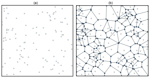
Figure 4 Positions of randomly placed sites (a) and the resulting generated Voronoi diagram of polygons (b).

The NetCDF file containing input data, created using ForeFire, is imported into the IGS using the Snappy Python library (How to use the SNAP API from Python, 2024). Snappy allowed for the NetCDF data to be read into Python arrays used for computation. The generated Voronoi diagram was overlaid on top of the NetCDF data. The elevation, wind, and fuel values (per fuel index) were recorded for every pixel in all polygons of the Voronoi diagram. This was done using the scan-line polygon fill algorithm to extract environmental data from the pixels contained within the polygon (Al-Rawi, 2014). The mean elevation, wind, and fuel values of each polygon were then saved.

The IGS starts with a fire located at the site of a Voronoi polygon. The propagation of this fire towards the site of each bounding polygon is modelled using the Rothermel model. When the fire reaches the site of a bounding polygon, the fire then progresses towards the new neighbouring polygons from that bounding polygon. Fires may propagate towards each other simultaneously. Fire progress is recorded as a ratio of how far it has propagated towards neighbouring polygon sites and the total distance between the two polygon sites. This is known as the propagation ratio. When the Rothermel model is run, the propagation ratio from the ignited polygon to its neighbours will increase if the rate of spread is positive (Fig. 5, Eq. 2). When the propagation ratio reaches 1, the neighbouring polygon will become ignited and will also begin spreading fire as this represents the fire spreading the entire distance between both polygon sites. The propagation ratio is calculated as follows:

$$\begin{array}{}\text{(2)}& {\left(P_{ij}\right)}_{t+\mathrm{dT}}={\displaystyle \frac{\left({\left(P_{ij}\right)}_t{d}_{ij}\right)+\left(R_{ij}\mathrm{d}T\right)}{d_{ij}}},\end{array}$$

where i is an ignited polygon, j is a polygon that neighbours the ignited polygon, t is the current time (s), dT > 0 is the time step (s), $\mathrm{0}\le (P_{ij}{)}_{t+\mathrm{dT}}\le \mathrm{1}$ is the propagation ratio between polygons i and j at time t+dT, $\mathrm{0}\le {\left(P_{ij}\right)}_t\le \mathrm{1}$ is the propagation ratio between polygons i and j at time t, R_ij ≥ 0 is the rate of spread between polygons i and j calculated by the Rothermel model (m s⁻¹), and d_ij > 0 is the distance between the sites of polygons i and j (m).

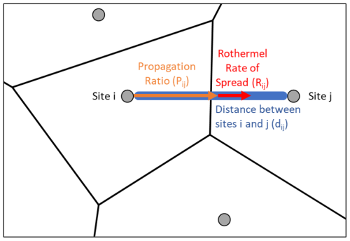
Figure 5 Example of the fire spreading from polygon i to j, where the blue line represents the total distance (d_ij) between sites i and j (m), the orange arrow represents the propagation ratio (P_ij) of how far fire has spread from site i to j, and the red arrow represents the fire's rate of spread determined by the Rothermel model (R_ij) from site i to j (m s⁻¹).

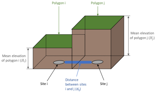
The Rothermel model requires data describing the fuel, the terrain's angle of slope, and wind. Every polygon has fuel data associated with it. The IGS uses the fuel data associated with the polygon the fire is spreading to during simulation. If the fuel data associated with the polygon the fire is spreading from were used, then fire would spread from that polygon to all its neighbours at an equal rate in conditions where there is no slope or wind. A weighted fraction between the two polygons was not used as it would create additional computational time for simulating a wildfire. Therefore, the fuel properties of the polygon the fire is spreading to were selected. The slope is found by getting the difference in elevation between the neighbouring polygon and ignited polygon, which is then divided by the distance between the polygon sites (Fig. 6):

$$\begin{array}{}\text{(3)}& S_{ij}={\displaystyle \frac{H_j-H_i}{d_{ij}}},\end{array}$$

where i is the ignited polygon, j is the neighbouring polygon, S_ij is the slope from i to j, H_j is the mean elevation of polygon j (m), H_i is the mean elevation of polygon i (m), and d_ij > 0 is the flat distance between the polygon sites i and j (m).

Figure 6 Variables used in Eq. (3) to determine the slope from polygon i to polygon j.

The normal wind value is used in the Rothermel model; it is found by getting the dot product between the wind vector and the unit vector describing the ignited polygon and neighbouring polygon sites' coordinates (Fig. 7):

$$\begin{array}{}\text{(4)}& {\left(W_{ij}\right)}_{\mathrm{n}}=\left[\begin{array}{c}{\left(W_j\right)}_{\mathrm{z}}\\ {\left(W_j\right)}_{\mathrm{m}}\end{array}\right]\cdot {\displaystyle \frac{\mathit{i}\mathit{j}}{∥\mathit{i}\mathit{j}∥}},\end{array}$$

where i is the ignited polygon's site, j is the neighbouring polygon's site, ${\left(W_{ij}\right)}_{\mathrm{n}}$ is the normal wind from i to j (m s⁻¹), ${\left(W_j\right)}_{\mathrm{z}}$ is the mean zonal wind speed of j (m s⁻¹), ${\left(W_j\right)}_{\mathrm{m}}$ is the mean meridian wind speed of j (m s⁻¹), and ij is the vector from polygon site i to polygon site j.

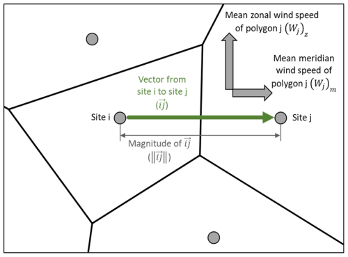
Figure 7 Finding the normal wind for fire spreading from site i to j by getting the dot product of both the mean zonal and meridian wind speed properties of polygon j and the unit vector of spread from site i to j.

A visualisation was created to show the spatial distribution of the polygons and evolution of the fire line. The polygons were rendered in distinct colours to represent their states, with red representing polygons that were currently on fire, black representing those that were completely burnt, clear without colour representing those that had not caught fire yet, and greening representing the wildfire source polygon(s) where the fire started. The colour of a polygon was determined from a combination of the masses in the states mentioned. A 50 % transparency was used to allow for the underlying map data to be seen (Fig. 8).

The produced Voronoi diagram was then scaled and overlaid on top of the satellite image so that each pixel coordinate in the Voronoi diagram would correspond to a pixel on the satellite image. The area of the polygon was then found in pixel coordinates and converted to an area in square metres (m²). For fire line calculations, the oven-dry fuel load per square metre (m²) was sourced from the fuel file and used to estimate the total fuel per polygon (kg). The total fuel in the polygon could then be split into flammable vegetation, currently ignited vegetation, and vegetation that had been completely burnt, written as

$$\begin{array}{}\text{(5)}& V_i=N_i-\left(I_i+B_i\right),\end{array}$$

where i is a polygon, N_i ≥ 0 is the total amount of fuel in polygon i (kg), V_i ≥ 0 is the amount of remaining flammable vegetation in polygon i (kg), I_i ≥ 0 is the amount of fuel in polygon i that is currently ignited (kg), and B_i ≥ 0 is the amount of fuel in polygon i that has burnt (kg). To estimate the mass of a polygon that was currently on fire, the propagation ratios from the ignited polygon and its neighbours were found. The total propagation ratios of fire that had spread within the ignited polygon only (both from that polygon and to that polygon), and the total half distances, between the ignited and neighbouring polygons were calculated. They were multiplied by each other and the total amount of fuel in the polygon to produce total amount fuel that had ignited. The amount of completely burnt fuel was then subtracted producing the fuel mass that was currently on fire:

$$\begin{array}{}\text{(6)}& {\displaystyle }{q}_{ij}=\left(P_{ij}\right)+\left(P_{ji}-\mathrm{0.5}\right),\text{(7)}& {\displaystyle }{I}_i=N_i{\displaystyle \frac{{\sum }_{j=\mathrm{1}}^{n_i}{q}_{ij}{d}_{ij}}{{\sum }_{j=\mathrm{1}}^{n_i}\frac{d_{ij}}{\mathrm{2}}}}-B_i,\end{array}$$

where i is a polygon, j is a polygon neighbouring i, q_ij ≥ 0 is the total propagation ratio of fire that has spread within polygon i between it and polygon j, N_i ≥ 0 is the total amount of fuel in polygon i (kg), I_i ≥ 0 is the amount of fuel in polygon i that is currently ignited (kg), B_i ≥ 0 is the amount of fuel in polygon i that has burnt (kg), 0 ≤ P_ij ≤ 1 is the propagation ratio from polygon i to j, 0 ≤ P_ji ≤ 1 is the propagation ratio from polygon j to i, n_i ≥ 0 is the number of neighbours polygon i has and d_ij > 0 is the distance between polygons i and j (m). Please note if q_ij > 0.5 then the value of q_ij is set to 0.5 and if P_ji < 0.5 then the value of P_ji is set to 0.5. This was to ensure only fire that had spread within polygon i was measured as any other spread in neighbouring polygons was used to find the mass of their polygon that was on fire instead.

The reaction intensity parameter from the Rothermel model found the energy produced per unit area per time step. Using the equation for the reaction intensity, the energy produced per unit mass per unit time step (E_ij) can be evaluated. This is done by removing the net fuel load ${\left(w_n\right)}_j$ from the equation Eq. (8) to give Eq. (9), which, as previously stated, uses United States customary units. E_ij was found using the fuel properties from neighbouring polygons and was converted to metric units.

$$\begin{array}{}\text{(8)}& {\displaystyle }{\left(I_{\mathrm{R}}\right)}_{ij}={\mathrm{\Gamma }}_j^{\prime }{\left(w_n\right)}_j{h}_j{\mathit{\eta }}_{{\mathrm{M}}_j}{\mathit{\eta }}_{{\mathrm{S}}_j},\text{(9)}& {\displaystyle }{E}_{ij}={\mathrm{\Gamma }}_j^{\prime }{h}_j{\mathit{\eta }}_{{\mathrm{M}}_j}{\mathit{\eta }}_{{\mathrm{S}}_j},\end{array}$$

where i is a polygon, j is a polygon neighbouring i, ${\left(I_{\mathrm{R}}\right)}_{ij}$ ≥ 0 is the reaction intensity of polygon j in J m⁻² s⁻¹ (Btu ft⁻² min⁻¹), ${\left(w_n\right)}_j$ ≥ 0 is the net fuel load of polygon j in kg m⁻² (lb ft⁻²), E_ij ≥ 0 is the energy produced spreading from polygon i to polygon j per mass per time increment in J kg⁻¹ s⁻¹ (Btu lb⁻¹ min⁻¹), ${\mathrm{\Gamma }}_j^{\prime }$ ≥ 0 is the optimum reaction intensity of polygon j per second (min⁻¹), h_j ≥ 0 is the low heat content of polygon j in J kg⁻¹ (Btu lb⁻¹), 0 ≤ ${\mathit{\eta }}_{{\mathrm{M}}_j}$ ≤ 1 is the moisture damping coefficient of polygon j, and 0 ≤ ${\mathit{\eta }}_{{\mathrm{S}}_j}$ ≤ 1 is the mineral damping coefficient of polygon j. Just like the base Rothermel model, Eq. (9) may have poorer performance in some fuel beds at lower fuel loadings, especially those with high packing ratios. Minor modifications were made to the Rothermel model that helped reduce the oversensitivity to fuel depth (Albini, 1976). This updated form of the Rothermel model was not used by the IGS as ForeFire used the base Rothermel model, which would make any comparison unfair.

The mean energy produced from burning fuel while the fire spread to its neighbouring polygons was calculated by multiplying the mean E_ij from all neighbouring polygons with the mass of ignited fuel in the polygon and the time step. The energy was then divided by the low heat content of the polygon to get the amount of ignited mass lost to burning:

$$\begin{array}{}\text{(10)}& {\mathrm{dB}}_i={\displaystyle \frac{\frac{\sum _{j=\mathrm{1}}^{n_i}{E}_{ij}}{n_i}{I}_i\mathrm{dT}}{h_i}},\end{array}$$

where i is a polygon, j is a polygon neighbouring i, E_ij ≥ 0 is the energy produced spreading from polygon i to polygon j per mass per time increment in J kg⁻¹ s⁻¹ (Btu lb⁻¹ min⁻¹), dB_i ≥ 0 is the rate at which ignited fuel in polygon i becomes burnt fuel in kg dT⁻¹, n_i > 0 is the number of polygons that neighbour i, I_i ≥ 0 is the amount of fuel that is currently ignited in polygon i in kilograms, dT > 0 is the time step in seconds, and h_i ≥ 0 is the low heat content of polygon i in J kg⁻¹ (Btu lb⁻¹). This value was then added to the total amount of fuel that has been burnt in that polygon:

$$\begin{array}{}\text{(11)}& {\left(B_i\right)}_{t+\mathrm{dT}}={\left(B_i\right)}_t+{\mathrm{dB}}_i,\end{array}$$

where i is a polygon, dT > 0 is the time step (s), dB_i ≥ 0 is the rate at which ignited fuel in polygon i becomes burnt fuel (kg dT⁻¹), t is time in the simulation (s), and ${\left(B_i\right)}_t$ ≥ 0 is the amount of fuel that is burnt in polygon i at t time (kg). Tracking both ignited and burnt fuel amounts paints a clear image of what areas are still on fire and which have ceased burning (Fig. 8).

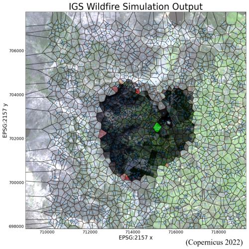
Figure 8 Sample simulation output after 100 000 s showing unburnt (transparent), wildfire source (green), burning (red), and burnt (black) polygons based on the mass of the polygon in that state, with a coloured satellite image of the terrain in the background (Copernicus 2022).

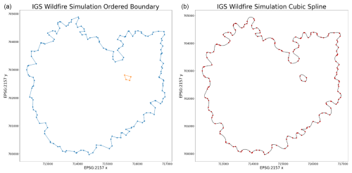
The boundary of ignited and burnt polygons can then be converted into a fire line, representing the outer perimeter of the fire. This allows for the IGS to be compared to other continuous programs such as ForeFire. The boundary polygons need to be found to produce a fire line. A straightforward algorithm was used to find the boundary polygons where each polygon was checked to see if it can spread the fire (a polygon is only able to spread fire if the fire spread model has reached that polygon's site). Once a set of polygons capable of spreading fire is found, it can be shortened by checking if these polygons have one or more neighbours that cannot spread fire. This gives an updated set of boundary polygons that are on the fire line perimeter of the IGS. This was then converted to a list containing boundary edges by checking the edges of each boundary polygon and recording any edges between a boundary polygon and a polygon that cannot spread fire. Getting the boundary edges of the boundary polygons helps reduce underpredicting how far the fire has spread within a given boundary polygon. Polygons that can spread fire while also touching the outer perimeter of the NetCDF file are checked, and any edges of that polygon on the perimeter were added to the list of boundary edges. Edges each consist of two vertices. To begin a random edge is selected from the list of boundary edges and a recursive algorithm finds the next edge to share vertices with the randomly selected edge, removing it from the list and storing it in a stack. This process is repeated until no more shared vertices can be found, and the stack then becomes an ordered boundary. The process of selecting a random edge continues until all edges have been removed from the list (Fig. 9). Sometimes the vertices of edges do not line up perfectly, so a 3 m (approximately 0.01 % of the region width) margin of error between vertices of different edges was allowed to ensure a completed shape. All edges shorter than the margin of error were removed to prevent inaccuracies caused by these small edges while generating the boundary.

The ordered boundary was then smoothened to provide the final representation of the fire line, using a cubic spline. The SciPy Python library has a subpackage called “interpolation” (Oliphant et al., 2024). This subpackage can be used to generate cubic splines given separate lists of x and y coordinates. Traditionally cubic splines are performed where x coordinates are ordered in increasing value. This will not work for the IGS's output as reordering the x coordinates would make the boundary unordered and ruin the boundary shape. To circumvent this, a parameter (c) was defined as the cumulative distance between all previous points in the ordered boundary. For example, the first point would have c equal to 0, while the second point would be equal to the distance between the first and second point. The third point would have c equal to the distance between the first and second point summed with the distance between the second and third point. Due to c being a list of increasing values, it was possible to perform a cubic spline on both the x and y coordinates separately using c (Cubic spline for non-monotonic data (not a 1d function), 2024). The x and y coordinates can then be re-combined to produce a cubic spline. With the cubic spline, the fire line becomes a smooth curve, more closely resembling how a real fire would appear (Fig. 9).

Figure 9 (a) Ordered boundary consisting of polygon edges from the IGS output that create an outer perimeter of the simulated wildfire. (b) Ordered boundary smoothened by a cubic spline.

3.3 Methodology to compare two wildfire outputs

A new method was developed to compare the similarity of outputted wildfires. This method took inspiration from both set theory and receiver operating characteristics (ROCs). When comparing outputted wildfires, one of the wildfires was treated as the ground truth. For this paper ForeFire was selected as the ground truth due to its increased resolution; therefore the IGS was selected as the predicted wildfire. The area of predicted fire that overlapped with the ground truth was treated as true positives. Areas where the IGS predicted fire and ForeFire did not were false positives. Areas where ForeFire predicted fire and the IGS did not were false negatives. Areas where both the IGS and ForeFire predicted there would not be fire were true negatives (Fig. 10). Unfortunately, the area of true negatives could be considered infinite, dependent on the size of the plane where the fire is being simulated. Therefore, true negatives were not counted and any confusion matrix calculations involving them were not used.

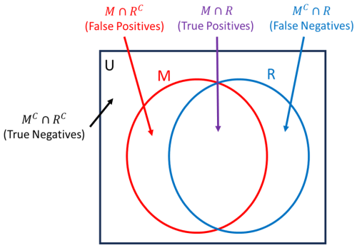
Figure 10 Calculating similarities of IGS (M) and ForeFire (R) wildfire shape outputs, where the area of M ∩ R is true positive, that of M ∩ R^C is false positive, that of M^C ∩ R is false negative, and that of M^C ∩ R^C is true negative.

The threat score was chosen as the metric of accuracy due to it measuring true positives, false positives, and false negatives simultaneously without requiring a measurement of true negatives. The default threat score equation was used, but two weighting factors were added to allow for the scaling of how important false positives and false negatives are relative to the true positives. It is given by

$$\begin{array}{}\text{(12)}& \text{TS}={\displaystyle \frac{\text{TP}}{\text{TP}+w_{\mathrm{1}}\text{FN}+w_{\mathrm{2}}\text{FP}}},\end{array}$$

where TS is the threat score, TP is the area of true positives, FN is the area of false negatives, FP is the area of false positives, w₁ ≥ 0 is the weighting coefficient for FN, and w₂ ≥ 0 is the weighting coefficient for FP.

If TS is 1, both the IGS and ForeFire polygons are a perfect match, while if TS is 0, there is no overlap between the IGS and ForeFire fire lines. Increasing w₁ or w₂ will make FN and FP respectively have a greater impact on lowering TS, while decreasing w₁ or w₂ will have the opposite effect. For the comparison of results in this paper, w₁ = w₂ = 1.

4 Comparison of grid types

Five different grid types were compared to find which grid type may be the optimal grid for comparison against ForeFire. All five grids were built using Voronoi diagrams. The five grid types consisted of randomly plotted sites; a triangular tessellating grid; a square tessellating grid; a hexagonal tessellating grid; and a grid where more sites would be plotted closer to the wildfire source and on land cover types defined by the fuel properties table, which are important to monitor. This grid is referred to as the flammable resolution grid (FRG). Each grid uses the von Neumann neighbourhood for determining which cells neighbour other cells (corner neighbouring cells exclusive) (Małecki, 2017).

The grid with randomly plotted sites takes as input the number of sites it must plot and a bounding box to plot the sites inside. It randomly plots that number of sites within the bounding box. If a site is plotted on top of an existing site, then that site will be re-plotted. Each polygon in the randomly plotted grid will have at least one neighbour with no maximum number of neighbours (Fig. 12).

The triangular grid consists of tessellating equilateral triangles of equal size. It uses a user-inputted number of sites it must plot and a bounding box to plot the sites inside. It is one of the more complicated grid types to plot using a Voronoi diagram. The program iterates through possible different numbers of sites to place on each row until it finds the optimal number. Using these values, it is possible to find the horizontal distance between sites and therefore the required vertical height of triangles on each column using the properties of equilateral and right-angled triangles (Fig. 12), through the following equation:

$$\begin{array}{}\text{(13)}& y=\sqrt{\mathrm{3}{x}^{\mathrm{2}}}=Y_{\mathrm{l}}+Y_{\mathrm{s}},\end{array}$$

where y > 0 is the height of the equilateral triangles, x > 0 is the horizontal distance between sites, Y_s > 0 is the short vertical offset, and Y_l > 0 is the long vertical offset. The program continues iterating until it finds the smallest number of sites to place in a row, where once the entire grid is filled vertically there will still be approximately the same number of sites as originally inputted. A short vertical offset is found to generate the triangular shape. The short vertical offset is calculated as the site for each equilateral triangle should be equidistant from all corners of the triangle. Therefore, using Pythagoras's theorem, the horizontal distance between sites, and the vertical height of the triangles, the location of these sites can be found by

$$\begin{array}{}\text{(14)}& {\displaystyle }{Y}_{\mathrm{l}}=x^{\mathrm{2}}+Y_{\mathrm{s}}^{\mathrm{2}},\text{(15)}& {\displaystyle }{Y}_{\mathrm{s}}=-{\displaystyle \frac{x^{\mathrm{2}}-y^{\mathrm{2}}}{\mathrm{2}y}},\end{array}$$

where Y_s > 0 is the short vertical offset, x > 0 is the horizontal distance between sites, y > 0 is the height of the equilateral triangles, and Y_l > 0 is the long vertical offset. In triangular tessellation on a singular row the triangles appear upright (generated from the short vertical offset) followed by an upside-down triangle in a repeating pattern. The upside-down triangles require the long vertical offset to be placed correctly. To find the long vertical offset the short vertical offset is taken away from the vertical height of the triangles (Fig. 11, Eq. 13). Where rows and columns are both indexed even or odd, the short vertical offset is applied. While on odd-indexed rows and even-indexed columns or even-indexed rows and odd-indexed columns, the long vertical offset is applied. This placement of sites creates a triangular grid. Due to rounding errors in Python and the Foronoi Python library, additional small edges were sometimes created between sites. To fix this, if the length of an edge was under a certain threshold, it was removed to prevent the grid from assuming some sites had additional neighbours (Fig. 12).

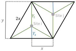
Figure 11 Calculation of Voronoi diagram site placement for equilateral triangular tessellation. Given the distances of x and y, Y_s and Y_l can be derived using the Pythagorean theorem.

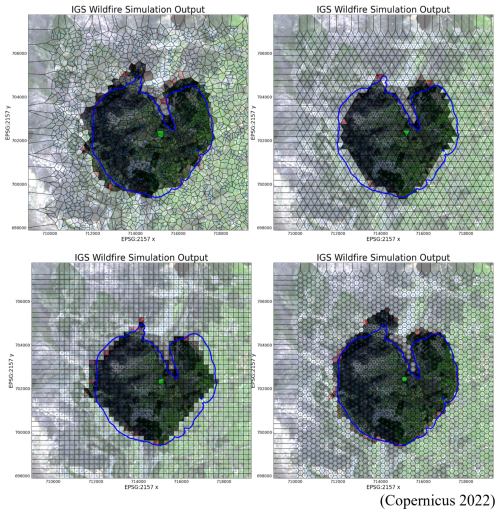
Figure 12 Outputs of different IGS grid types (coloured polygons) compared to ForeFire's output (blue). On the top left are randomly plotted sites, on the top right is a triangular grid, on the bottom left is a square grid, and on the bottom right is a hexagonal grid (Copernicus 2022).

The square grid consists of tessellating squares in a chessboard pattern, where the squares are all of an equal size and aligned both horizontally and vertically. It uses the user-inputted number of sites and a bounding box to plot the sites inside. The floored square root of the number of sites to plot is found and is used to equally space sites within the bounding box into equidistant columns and rows. Each polygon in the square grid (not on the edge) will have four neighbours (Fig. 12).

The hexagonal grid consists of tessellating regular hexagons of an equal size defined by the user-inputted number of sites and a bounding box. Like the triangular grid, the program iterates through possible different numbers of sites to place on each column until it finds the optimal number. The optimal number of points to place is found by getting a number as close to what was originally stated within the bounding box, as the horizontal distance between sites could be found given the vertical distance, i.e.

$$\begin{array}{}\text{(16)}& x=\sqrt{y^{\mathrm{2}}-{\left({\displaystyle \frac{y}{\mathrm{2}}}\right)}^{\mathrm{2}}},\end{array}$$

where x > 0 is the horizontal distance between sites and y > 0 is the vertical distance between sites. Every even column is then offset vertically by half the vertical distance between sites. Each polygon in the hexagonal grid (not on the edge) will have six neighbours (Fig. 12).

A random grid with increased focus on a region of interest was created called the FRG. It was designed to have a greater density of sites in regions most likely to be affected by wildfire and regions that are important to monitor. The regions that are most likely to be affected by wildfires tend to be situated closer to the ignition point of the fire or contain land cover types that can sustain large fires (e.g. forested areas). Areas of preselected importance tend to be areas with a higher density of people (e.g. urban areas). To do this the program runs through each pixel of the land cover map within the bounding box where it has a base probability of selecting the pixel it is currently on (this ensures that not too many sites are generated). Once a pixel has been selected a second probability is generated to determine if a site should be placed at this position based on the distance from the ignition point and the land cover type of that pixel:

$$\begin{array}{}\text{(17)}& G=F(\mathrm{1}+m{)}^{-k},\end{array}$$

where 0 ≤ G ≤ 1 is the probability of a site being placed, 0 ≤ F ≤ 1 is the coefficient affecting the probability of site placement based on land cover type, m ≥ 0 is the distance between the current pixel and the mean ignition point divided by the distance between the ignition point and furthest point within the bounding box, and k > 0 is a coefficient that weighs site placement probability based on 1+m. This allows for most of the computing to be performed where it is most likely to be needed instead of wasting resources in areas the fire is unlikely to reach or to spread fast in. Each polygon in the FRG will have at least one neighbour with no maximum number of neighbours (Fig. 13).

A fire was set using EPSG:2157 coordinates (715122, 702388) at 0 s in the simulation. The environment had no wind, and the fire was simulated for 100 000 s with a time step of 1000 s. The fire was simulated 10 times for each grid type, where the time it took for the IGS to simulate the fire and the threat score were both recorded (Table 1). Values for the equation of site placement of the FRG were selected so the FRG would have approximately 2000 sites each time.

Table 1 Number of sites, threat scores, and simulation times for the different grid types. All grid types excluding the FRG have a constant number of sites. All grid types except the random grid and FRG have a constant threat score.

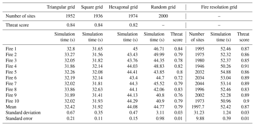
The regular grids and the random grid had a set number of sites, while the FRG had a varying level of sites due to the nature of its site generation. As the regular grids were deterministic, each simulation produced the same wildfire and therefore their threat score was constant throughout, unlike the random grid and FRG. The regular grids tend to have quicker execution times than the random grid and FRG, where the FRG has the longest simulation time. The random grid and FRG also have significantly higher standard deviations and standard errors in their simulation time; this is due to both grids generating a completely new grid layouts each time the simulation is run, while the regular grids always have the exact same grid layout. The random grid had the lowest threat score, while the FRG had the highest threat score.

The triangular, square, and hexagonal grids can estimate the shape of the fire line well as shown by their threat scores, but they are confined to their regular shape and may struggle to represent some of the more irregular shapes of actual fire lines. As the von Neumann neighbourhood was used to define neighbours, the regular grids all share the property of having an equal number of neighbours (not on the bounding box edges) that are all equidistant from each other, which gives all polygons an equal spreading opportunity (Fig. 12). The regular grids had an equal resolution across the entire grid. This leaves room for further optimisation where areas less likely to burn according to the model could have a lower resolution.

The randomised Voronoi grid can produce some of the more irregular shapes, which can allow it to follow the irregular pattern of real terrain. Unlike the regular grids each polygon does not have an equal spreading opportunity due to the distance between neighbouring sites varying. The randomised Voronoi grid has a similar resolution throughout the grid, which was not an optimal use of computation power. The FRG can follow the shape of the fire line with greater precision due to its high resolution in areas of importance. It also decreases computational waste due to it rendering smaller numbers of polygons in areas of little importance. It does not have an equal spreading opportunity for each polygon and takes longer than all other types of grids to simulate the spread of fire (Fig. 13).

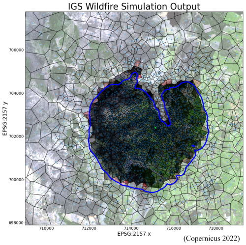
Figure 13 Output of the flammable resolution grid (coloured polygons) compared to ForeFire's output (blue) (Copernicus 2022).

Due to the greater resolution of the FRG, it will be used in the remaining comparisons in this paper. To find how effective the IGS was at simulating wildfires, it was then compared to the industry-standard wildfire-modelling program ForeFire.

5 Summary of results

To compare the IGS and ForeFire, 20 wildfires were simulated. The wildfires were randomly placed in various locations within the Wicklow Mountains, Ireland, with varying wind speeds and for different durations. This was done to test the versatility of the IGS. Some simulations included multiple separate wildfires. Outputs of ForeFire and the cubic spline of the IGS using the FRG were graphed, and then their similarity was found (Fig. 14). While simulating these wildfires the time it took to run the simulation of the IGS usually took longer than ForeFire, even though it required less computing. This was due to ForeFire being built in the more computationally efficient language C$++$ (Zehra et al., 2020). To make the comparison between the IGS and ForeFire fair, the main simulation loop of the IGS was ported to C$++$ from Python. The remaining code for the IGS was still in Python. The comparison does not include the setup times for ForeFire or the IGS.

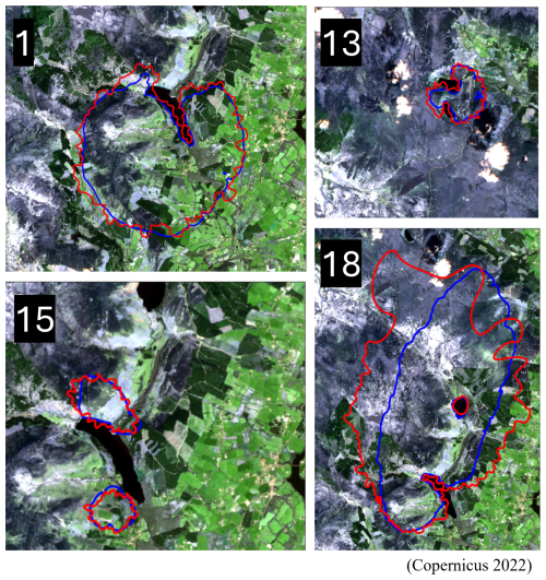
Figure 14 IGS output (red) compared to ForeFire output (blue) (top left: wildfire 1, top right: wildfire 13, bottom left: wildfire 15, bottom right: wildfire 18; Table 2) (Copernicus 2022).

The time it took to run the main simulation loops of ForeFire and the IGS in both Python and C$++$ were recorded and compared. The areas of true positives, false positives, and false negatives for the IGS when compared to ForeFire were recorded for each wildfire, and the corresponding threat score was calculated. These data are presented in Table 2.

Table 2 Comparison of 20 simulated wildfires in ForeFire and the IGS under the metrics of computing time (ForeFire/IGS C$++$ time) and similarity of the resulting fire line (threat score, where w₁, w₂ = 1).

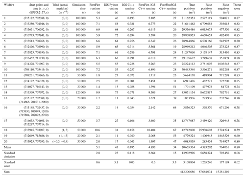
From the sample wildfires simulated, the IGS runs on average 34 times more quickly than ForeFire, with a mean fire line similarity of 0.8 when compared to ForeFire. The use of the IGS instead of ForeFire allows for multiple wildfires to be simulated (restricted to one area) in the same amount of time it would take ForeFire to run a simulation of one wildfire. From Table 2 it is evident that the fire lines produced by the IGS when compared to their ForeFire counterpart tended to contain mostly areas of true positives followed by false positives and finally false negatives. There is also a trend where IGS-simulated wildfires that are run for longer durations tend to not perform as well as those run for shorter durations relative to ForeFire. Adding wind or additional wildfire sources in the comparison does not impact the relative computing time or similarity to ForeFire. There are some limitations with the IGS, however. The FRG can have problems with larger wildfires as the frequency of polygons decreases the further a wildfire spreads from its ignition point. This is evident in wildfire 18 (Fig. 14), where there is a large drop in site resolution at distances far away from the wildfire-starting location. The large distance between the IGS and ForeFire's northern and western fire lines highlights this issue. The cubic spline used forces the curve to intersect the points on the edges of polygons. Due to the resolution of sites within the IGS, this makes the cubic spline produce small modulations on the fire line, while ForeFire has straighter edges.

6 Discussion

Comparing the five different grid types produced a table of computational times and the similarity of their outputs relative to ForeFire (Table 1). Overall, the regular grids produced the same output every time the program ran, making them deterministic. They also took approximately the same time to run the simulation as shown by the small standard deviation in their computational times. The small standard deviation can be accounted for with other uncontrollable minor factors affecting the computer such as background tasks. Both irregular grids have a much higher standard deviation in their computational times. This is because the process of seeding these grids is non-deterministic, so a different grid is produced each time a simulation is run. Some of the irregular grids have overall regions of higher resolution than others, which can lead to varying computational times. The number of neighbours each grid has is also correlated to the computational time, as the program must calculate the propagation ratio between each ignited polygon that can spread fire to its neighbour. The square and triangular grids have the fastest computational times while having four and three neighbours respectively. The hexagonal grid has the next fastest computational time with six neighbours. The random grid has a computational time very similar to that of the hexagonal grid, even though there is no set number of neighbours per polygon. This is most likely due to each polygon having approximately six neighbours. The FRG has the slowest computational time, even though most polygons also have approximately six neighbours. This is due to the increased density of polygons close to the wildfire source, as propagation ratios need to be calculated for all these ignited polygons and their neighbours that fire can spread to. In terms of the similarity of output to ForeFire, the FRG performs the best followed by the square, triangular, hexagonal, and random grids. As previously mentioned, the FRG has a high density of polygons near the wildfire source, allowing for the simulation to nearly follow the continuous movement of the wildfire simulated in ForeFire. For the regular grids to be comprised of regular shapes (and equilateral triangles in the case of the triangular grid) it was only possible to have a set number of polygons in the simulation area. In the table, the number of sites for the regular grids was set as close to 2000 as possible while still retaining a regular grid. The disparity in the number of polygons between the grids can explain some of the differences in similarities with ForeFire. The irregular random grid tends to produce outputs with the lowest similarity to ForeFire's compared to any other grid. This may be due to the minor variations in cell sizes within the random grid. The regular grids have a set number of directions fire can spread in to reach neighbouring polygons; they also struggle with following the irregular patterns in Earth's terrain as seen by the lake (Fig. 12). Overall, there is no definitive best grid type. It really depends on what the user is trying to simulate and how detailed they are willing to have the simulation be in exchange for more computational time. In this paper the FRG was chosen as it produced results most like ForeFire's.

Comparing the IGS and ForeFire produced a table examining the computational efficiency and similarity of their outputs (Table 2). ForeFire is deterministic and therefore produces the same results every time it is run. In this comparison the IGS was using the FRG grid, which is non-deterministic. The IGS wildfires that ran for shorter durations tended to be computationally faster than the wildfires that ran for longer durations, relative to ForeFire. This is caused by the increasing size of the simulated wildfire as it burns, resulting in more ignited polygons that can spread fire to their neighbours, therefore creating additional computational burden per iteration. The IGS produces a larger area of false positives than that of false negatives when compared to ForeFire; this is due to the fire line selection process. As the IGS selects the fire line from the outer edges of the polygon if fire has reached that polygon's site, regardless of how far the fire has spread within that polygon to its surrounding edges, it sometimes overestimates the distance the fire has spread. This is the reason for a larger area of false positives than false negatives when compared to ForeFire. The threat score for similarity between the IGS and ForeFire increases with the length of simulation. This is due to the overall area of the wildfire, which tends to be mostly true positives, growing at a faster rate than the boundary of the wildfire where false positives and false negatives tend to occur.

7 Conclusion

A novel software platform that allows for the change of grid type using simple parameterisation for wildfire modelling was developed. This allowed for grids to be compared within the same framework. The software included irregular grids constructed from Voronoi diagrams. The approach of using irregular grids to predict the spread of wildfires allows for efficient computing while retaining a reasonable level of similarity to existing methods in results defined by the threat score. Existing software such as ForeFire can produce more precise simulations as it models fires in continuous space by moving markers representing the fire line, instead of simulating the spread of fire on a fixed grid determined before running the simulation. The use of continually moving markers requires additional computational time. The spatial resolutions of both programs must be noted however as ForeFire has a spatial resolution of 30 m² throughout, while the FRG has a varying spatial resolution with a maximum resolution of 10 m². The IGS has been incorporated into DecaMap's Common Operational Picture software platform, an application that has potential to assist with wildfire management (DecaMap, 2024).

The software has a few issues that could be improved in future work. A better form of site placement than the FRG could be developed to prevent the resolution of site placement decreasing at such a high rate at distances further from the wildfire source. A higher resolution could also be used to reduce the modulated boundary pattern produced by the cubic splines when converting the IGS output to a line. Porting the rest of the IGS from Python to a more computationally efficient programming language such as C$++$ would speed up the setup process for the IGS, making the overall software more efficient.

For the results ForeFire was treated as the ground truth as its continuous nature can be made to produce results of a higher resolution than that set in the IGS experiments. Both approaches use the same fire progression model. ForeFire could be considered an industry standard as it is commonly referenced in relevant literature (Kaur et al., 2016; Farguell et al., 2019; Trucchia et al., 2019).

This paper compared different grid types. It was shown that the FRG is the best option for greater resolution near the wildfire source. The regular grids are a better choice for more efficient computation. The decision of which grid type to choose should be made on a case-by-case basis by the user. The paper also showed that the IGS runs approximately 34 times more quickly than ForeFire, with a mean similarity of 0.8. While ForeFire will always produce wildfire simulations at a greater spatial resolution than the IGS, if computational efficiency is a concern where multiple wildfires may need to be simulated at one location, the IGS may end up being an alternative option.

Appendix A

A nearly cloud-free satellite image (product) taken by the Sentinel-2 satellite in April 2022 was downloaded from the European Space Agency (ESA) Sentinel Hub portal, a satellite image hosting platform (https://www.sentinel-hub.com/explore/eobrowser/, last access: 25 January 2024). Sentinel-2 products contain multiple bands which capture electromagnetic radiation (light) reflected off Earth's surface. A Level-1C product (top-of-atmosphere reflectance values) was used in this study. The data were then atmospherically corrected to bottom-of-atmosphere values using the Semi-Automatic Classification Plugin in the geographic information software QGIS which follows the dark-object subtraction (DOS) algorithm (Chavez, 1988; QGIS, 2024; Gilmore et al., 2015). This is due to Level-1C products originally containing information regarding both Earth's surface and atmosphere which may not accurately depict the actual conditions on the surface of Earth. Three additional indices for highlighting vegetation, urban areas, and soil (i.e. normalised difference vegetation index (NDVI), normalised difference built-up index (NDBI), and normalised difference tillage index (NDTI) respectively) were generated from the original Sentinel-2 bands. These indices are simple ratios calculated from the original multispectral bands and are known to help distinguish various land cover classes, i.e. NDVI for vegetation, NDBI for urban areas, and NDTI for bare soil. NDVI is a ratio between the red and near-infrared bands, whereas NDBI is calculated from the shortwave infrared (SWIR2) and near-infrared bands (Sun et al., 2019; Kebede et al., 2022). The tillage index (NDTI) is calculated from both the available SWIR bands (SWIR1 and SWIR2) (Sun et al., 2019). Areas of known land cover in the Wicklow Mountains, Ireland, were digitised to generate 70 polygons in total, which were further equally split into two sets. The first set was used to train a model, and the other was used as an independent validation of the predicted land cover class map. The training and validation datasets had 35 polygons each, which totalled to an area of 1.45 and 1.4 km² respectively. The polygons were selected in a manner to ensure a coverage of the entire study area, with separation between the polygons (avoiding extremely close areas for both training and validation) and intra-class variability for avoiding bias in the model. A supervised random forest algorithm was applied on the stack of seven original bands (red, green, blue, near-infrared (NIR), NIR narrow, shortwave infrared (SWIR1 and SWIR2)) captured by the Sentinel-2 satellite and the three additional indices to predict the land cover classes. A supervised random forest algorithm was then applied on the stack of seven original bands (red, green, blue, near-infrared (NIR), NIR narrow, shortwave infrared (SWIR1 and SWIR2)) captured by the Sentinel-2 satellite and the three additional indices to predict the land cover classes. The random forest classification algorithm is non-parametric in nature and known to improve estimates by averaging outputs from multiple decision trees randomly subset from the data. It has been successfully used for land cover mapping in previous studies, and the algorithm was run using the RStoolbox library in the R programming environment (Sibanda and Ahmed, 2021; Abdi, 2020; Pringle et al., 2018). The cloud-covered pixels in the area were classified based on a simple thresholding of the blue band (Baetens et al., 2019). The predicted land cover map was compared against the validation dataset which provided an overall accuracy of 97 %. The predicted land cover map for the area under study is shown in Fig. A1.

Figure A1 On the left is a Sentinel-2-based true-colour image of the study area, and on the right is a predicted land cover map for April 2022 (Copernicus 2022).