Is higher resolution always better? A comparison of open-access DEMs for optimized slope unit delineation and regional landslide prediction

Digital elevation models (DEMs) play a key role in slope instability studies, ranging from landslide detection and recognition to landslide prediction. DEMs assist these investigations by reproducing landscape morphological features and deriving relevant predisposing factors, such as slope gradient, roughness, aspect, and curvature. Additionally, DEMs are useful for delineating map units with homogeneous morphological characteristics, such as slope units (SUs).

In many cases, the selection of a DEM depends on factors like accessibility and resolution, without considering its actual accuracy. In this study, we compared freely available global elevation models (Advanced Land Observing Satellite (ALOS) World 3D-30m, Copernicus GLO-30 (COP), Forest And Buildings removed COP DEM (FABDEM)) and a national dataset (TINITALY) with a reference model (local airborne lidar) to identify the most suitable DEM for representing fine-scale morphology and delineating SUs in the Marche region, Italy, for landslide susceptibility studies. Furthermore, we proposed a novel approach for selecting the optimal SU partition.

The DEM comparison was based on several criteria, including elevation, residual DEMs, roughness indices, slope variations, and the ability to delineate SUs. TINITALY, resampled at a 30 m×30 m pixel size, was found to be the most suitable DEM for representing fine-scale terrain morphology. It was then used to generate the optimal SU partition among 18 combinations. These combinations were evaluated using both existing and newly integrated metrics alongside mapped landslide inventories to optimize terrain delineation and contribute to landslide susceptibility studies.

1 Introduction

Open-access global digital elevation models (DEMs) have been commonly used for a vast range of geomorphological studies, which have required modeling or analysis of terrain surface in mountain environments, where these DEMs have been characterized by a marked quality deterioration (Guth et al., 2024; Trevisani et al., 2023a). One of the many uses of DEMs has been to serve as the base input for analyzing landslide morphological features, evaluating the state and type of activity, and generating landslide susceptibility models (Brock et al., 2020). Among multiple methods of data-driven (Ahmed et al., 2023; Lombardo et al., 2020; Lombardo and Tanyas, 2020; Titti et al., 2021a) and physical-based models (Van den Bout et al., 2021) to predict, investigate (Brenning, 2005; Pirasteh and Li, 2017; Steger et al., 2023), and detect landslides (Qin et al., 2013), the elevation model has been of essential importance. DEMs are utilized to derive terrain-based characteristics (Brock et al., 2020; Mahalingam and Olsen, 2016), which have been conditioned by their resolution. In the literature, DEM resolution and its influence have been tested in several aspects, such as in landslide modeling and hazard assessment (Catani et al., 2013; Claessens et al., 2005; Fenton et al., 2013; Huang et al., 2023), in 3D physical models (Qiu et al., 2022), and in morphological quality assessment explored at regional scales (Grohmann, 2018; Hawker et al., 2019; Trevisani et al., 2023a).

Comparisons among DEMs to evaluate the most suitable product are based on different criteria, and the results have likely varied as per the test site. Thus, even if the same criteria have been used to rank DEMs, regional topography has influenced the preference of the elevation model in different areas (Florinsky et al., 2019; Zhang et al., 2019). Land cover has been particularly important when global DEMs (Bielski et al., 2024), such as the Copernicus GLO-30 (COP) and the Advanced Land Observing Satellite (ALOS) World 3D-30m, have been used to derive a digital terrain model (DTM), given that most of the time these products resemble a digital surface model (DSM; Guth and Geoffroy, 2021).

An ongoing initiative, the Digital Elevation Model Intercomparison eXercise (DEMIX; Strobl et al., 2021), has aimed to align methodologies, allowing for criteria-based ranking of global DEMs. In the first application (Bielski et al., 2024), metrics related to slope and roughness have been considered in addition to those related to elevation differences; the approach has been developed further, adopting new metrics and a wide range of geomorphometric derivatives (Guth et al., 2024). Global DEMs have been commonly used in geoscientific research due to their spatial extent and public accessibility, whereas national DEMs (Gesch et al., 2018; Muralikrishnan et al., 2013; Tarquini et al., 2007) have generally been tailored to represent country-specific land surface and morphology at a higher spatial resolution and accuracy to serve geoscience applications. The Shuttle Radar Topography Mission (SRTM; Jarvis et al., 2008), ALOS (Takaku et al., 2014), and the Terra Advanced Spaceborne Thermal Emission and Reflection Radiometer Global DEM (ASTER GDEM; Abrams et al., 2010) have been among the most widely used, freely accessible, and initial global DEMs utilized in geomorphic analyses (Becek, 2014; Florinsky et al., 2019; Mahalingam and Olsen, 2016; Trevisani et al., 2023a; Zhang et al., 2019). However, several factors must be considered when implementing these global datasets in a localized area for landslide recognition, mapping, and assessment.

Landslide inventories and elevation models have been essential inputs for data-driven landslide models, for which the DEM has been used to derive morphological parameters such as slope angle and slope aspect. For these derivatives to be as accurate as possible in a model, the DEM quality (Claessens et al., 2005; Mahalingam and Olsen, 2016; Saleem et al., 2019) should satisfy the representation of fine-scale morphology (Chaplot et al., 2006; Florinsky, 1998). In other words, the DEM quality significantly affects the prediction capacity of a model. The errors contained within a DEM, even when small, propagate in derivatives of elevation (Karakas et al., 2022; Mahalingam and Olsen, 2016; Pawluszek and Borkowski, 2017; Saleem et al., 2019), which have been weighed as important factors in landslide occurrence. The various available DEMs have been generated using a range of technologies. While significant efforts have been made to improve DEMs over time, the accuracy of these models has remained a critical issue. Selecting an appropriate DEM has proven to be more important than the number of DEM-derived factors used in landslide assessment (Kamiński, 2020).

Another use of DEMs has been the delineation of mapping units (Schlögel et al., 2018). Mapping units have been used to subdivide the study area into homogeneous, elemental units, such as administrative units (Lombardo et al., 2019), terrain units (Van Westen et al., 1997), unique condition units (Titti et al., 2021b), grid cells (Reichenbach et al., 2018), and slope units (SUs) (Ahmed et al., 2023). SUs were initially introduced by Carrara et al. (1991) as portions of territory, presenting homogeneous morphological characteristics for landslide identification and susceptibility mapping. The SU, according to the scale adopted, has served as a solution that adequately represents unstable slopes.

To assess the suitability of DEMs for landslide susceptibility and prediction, it has been essential to conduct a quality assessment of these models, which has commonly referred to the spatial resolution alone. Therefore, global DSMs and a national Italian DTM have been compared with a local accurate elevation model (airborne lidar) in the context of terrain representation and its delineation. The Italian DTM has already been investigated in some studies, mainly focusing on hydrogeomorphology studies (Pulighe and Fava, 2013; Zingaro et al., 2021; Annis et al., 2020; Tavares da Costa et al., 2019). Accordingly, quality evaluation from the perspective of fine-scale morphology and geomorphometric derivatives in the context of landslide science has remained an interesting aspect to explore further.

This study aimed to optimize inputs used for representing morphological data in landslide susceptibility assessment and to understand their interactions by identifying the most suitable DEM for accurately representing fine-scale slope morphology, proposing a new metric for analyzing optimal SU parameters for landslide susceptibility mapping, integrating landslide inventory data with landslide area and number, and extending and applying the methodology to test landslide susceptibility at a regional scale in the Marche region of central Italy.

2 Study area

In this study, we have selected two distinct study areas. The first area of interest (AOIa) encompasses the entire Marche region, located in central-eastern Italy (Fig. 1, AOIa). From a morphological point of view, this region is characterized by three different types of landforms that extend in the north–south direction. In the western part, the region is crossed by the Apennines, which can reach, in this area, a peak of 2476 m a.s.l. at Monte Vettore. In the central part of the region, the reliefs degrade to more rounded hills up to the flat eastern coastal strip. From a geological perspective, the Apennines, a Neogene fold-and-thrust belt that formed following the closure of the Mesozoic Tethys Ocean, are characterized by calcareous, calcareous–marly, and arenaceous units, as well as pelitic–arenaceous and marly–arenaceous units, ranging in age from the Jurassic to the Neogene. Several small rivers traverse the region from west to east. In particular, the basins of the Misa, Esino, Cesano, and Metauro rivers were affected by an exceptional thunderstorm in September 2022, triggering floods and landslides (Corti et al., 2024). One of the highest rainfall intensities of the 2022 event was registered in a sub-portion of the Marche region, which has been selected as the second study area (AOIb) for this work (Fig. 1, AOIb). This selection is based on not only the consequences of the exceptional rainfall event but also the fact that, morphologically, it is typically representative of the mountainous terrain of Marche. Moreover, this area is covered by a high-resolution dataset (1 m pixel size), which allows us to effectively conduct the experiments as described later in this work.

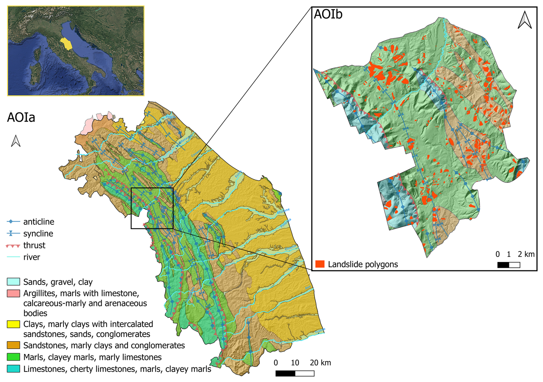
Figure 1 Study area in central Italy. On the left is the study area AOIa, encompassing the entire Marche region, which was analyzed in the second phase of the study. The geological classification is ordered by age (Quaternary, Cretaceous–lower Pliocene, lower Pliocene–lower Pleistocene, middle–upper Miocene, upper Eocene–upper Miocene, upper Trias–middle Eocene). On the right is the study area AOIb, a sub-portion of the Marche region where we conducted the DEM analysis in the first phase covered by the 1 m pixel size airborne lidar survey. The Piano Stralcio per l'Assetto Idrogeologico (PAI) landslide inventory of the Marche region identifies 19 296 landslide bodies as polygons. The top-left image background is from © Google Maps 2019.

A relevant portion of the territory of the Marche region (AOIa) presents slope failures. The most populated dataset of landslides in the area is the inventory of the Piano Stralcio per l'Assetto Idrogeologico (PAI) of the Marche region (Fig. 1). In the area of the Marche region (AOIa), the PAI counts 19 296 inventoried landslides for a total landslide area of 1394 km², which covers 15 % of the total regional surface classified as flow, slide, and complex landslides (Cruden and Varnes, 1996).

3 Materials and methods

The methodology implemented in this study aims to assess the quality of freely available DEMs, framing their use in landslide susceptibility assessment. DEMs have been essential because they allow for the derivation of landslide-predisposing factors and generate a morphology-based terrain subdivision: SUs. Thus, these two uses of a DEM in landslide susceptibility assessment have been investigated.

The analysis has been conducted in two sequential phases (Fig. 2). In the first phase, the differences in DEM derivatives were assessed by comparing global DEMs and a national DEM to a local high-resolution reference elevation dataset in AOIb. In the second phase, we evaluated 18 SU partitions on the basis of internal and external homogeneity, landslide extension, and landslide number using the best-performing open-source DEM, which was identified in the first phase of this study.

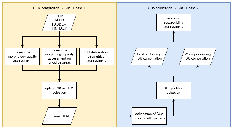
Figure 2 Workflow of the two-phase analysis. Phase 1 DEM assessment: comparison of global DEMs and a national DEM to a local high-resolution reference elevation model (with reference to AOIb). Phase 2 slope unit delineation: selection of the optimal parameters for SU delineation (with reference to AOIa).

3.1 Phase 1: DEM assessment

In this phase, the accuracy of three global DEMs, as mentioned below, and one national DEM (TINITALY) was evaluated through a comparison with a local airborne lidar in the study area AOIb.

ALOS (ALOS World 3D – 30m; https://doi.org/10.5069/G94M92HB, OpenTopography, 2024) was released by the Japan Aerospace Exploration Agency (JAXA) in 2015, at a horizontal resolution of 1 arcsec or approximately 30 m as a DSM (Caglar et al., 2018). This product, surveyed from 2006 to 2011, uses the 5 m mesh of World 3D topographic data and is provided in two resampled versions by JAXA (mean resampling kernel is used in this study), with elevation expressed according to the Earth Gravitational Model 1996 (EGM96).

COP (European Space Agency, 2024) was obtained from WorldDEM at 1 arcsec as a DSM, a product of the radar data acquisition of the 12 m TanDEM-X mission from 2011 to 2015. The Forest And Buildings removed COP DEM (FABDEM; Hawker et al., 2022) was made available as a corrected global DTM available at 1 arcsec grid spacing (60° S–80° N) derived from COP. Machine learning techniques have been devised to improve mean absolute vertical error in built-up and forested areas in comparison to COP (Hawker et al., 2022). Both FABDEM and COP elevations have been referenced to the EGM 2008 geoid.

TINITALY versions 1.0 (Tarquini et al., 2007) and 1.1 (Tarquini et al., 2023) cover the entire Italian territory as a DTM available at a 10 m pixel size. Heterogenous data, mainly based on regional technical cartography (CTR) with elevations derived by means of a photogrammetric method, have been used to build a national-scale model. In particular, the CTR map scaled at 1:10 000 with a 10 m interval for contour lines is used for the Marche region in the compilation of TINITALY. A triangular irregular network (TIN) structure has been employed in constructing the DEM to tackle varying data densities and redundancies. Merging various types of input data is followed by significant investigation to ensure the seamless production of a high-resolution (and potentially the most accurate) representation of Italy, with a root mean square error ranging from 0.1 to 6 m (Tarquini et al., 2007).

The reference DEM (as it is referred to hereafter) is a DTM that was acquired in 2012 using airborne lidar. It has a pixel size of 1 m×1 m and a reported vertical and planimetric accuracy of 15 and 30 cm, respectively (Ministero dell'Ambiente e della Sicurezza Energetica, https://gn.mase.gov.it/portale/pst-dati-lidar, last access: 2 July 2025). This reference DEM was aggregated by averaging the pixel size to 30 m.

The global DEMs (COP, FABDEM, ALOS) and TINITALY were projected to WGS84 UTM 33N, with pixel sizes of 30 and 10 m, respectively, using bilinear interpolation to align with the reference DEM. The inclusion of COP and FABDEM, along with ALOS as a global DEM and TINITALY as a national-scale elevation model for comparison, has been adopted by several studies (Bielski et al., 2024; Guth and Geoffroy, 2021; Meadows et al., 2024; Osama et al., 2023; Trevisani et al., 2023a). All the DEMs, except TINITALY (geoid model not publicly available), have been transformed into a common geoid model, EGM2008, for alignment and comparison with the reference grid. TINITALY is based on the Italian geodetic network (IGM95) where the measured ground points have been described by the Italian geoid called ITALGEO 2005 (Albertella et al., 2008; Barzaghi et al., 2007). Barzaghi and Carrion (2009) have concluded that the difference between ITALGEO05 (regional geoid model) and EGM2008 (global geoid model) is negligible for many applications, and both are capable of representing the region of Italy. Therefore, no geoid transformation for TINITALY is required.

To perform the quality assessment of selected DEMs, elevation differences were considered for compatibility with previous studies. Indeed, studies focusing on DEM comparisons (Polidori and El Hage, 2020) are generally based on elevation differences, using standard statistical metrics such as standard deviation and root mean square error (RMSE), and, in some cases, slope and aspect have been considered (Meadows et al., 2024; Zhang et al., 2019). However, as suggested in many studies (Bielski et al., 2024; Crema et al., 2020; Florinsky et al., 2019; Gesch, 2018; Guth and Geoffroy, 2021; Kakavas et al., 2020; Liu et al., 2019; Purinton and Bookhagen, 2017; Trevisani et al., 2023a), statistical metrics of elevation differences alone fail to fully capture the quality of DEMs, including the capability to represent fine-scale morphology and the presence of artifacts. Therefore, for this reason and because the focus of this work is primarily on investigating the accuracy of the DEMs' geomorphometric derivatives, along with the differences in elevation, a straightforward and simple approach has been proposed to take the local spatial variability of surfaces into account based on a geostatistical-based methodology (Isaaks and Srivastava, 1989), as discussed by Trevisani et al. (2023a).

The approach is based on the derivation of a residual DEM, also known as the topographic position index (TPI; Guisan et al., 1999; Hiller and Smith, 2008; Wilson and Gallant, 2000), and the calculation of roughness indices. The residual DEM, derived by detrending the original surface, enables us to highlight the capability of DEMs to reproduce local fine-scale morphology. Moreover, the residual DEM has been used as input for the calculation of roughness indices, such as the standard deviation of residual DEM (Grohmann et al., 2011), or even geostatistically based estimators, such as a variogram (Eq. 1, with p=2) and madogram (Eq. 1, with p=1). Equation (2) represents the more robust median absolute differences (MADs; Trevisani and Cavalli, 2016; Trevisani and Rocca, 2015). The generalization of the variogram is described in Eq. (1) and MAD in Eq. (2):

$$\begin{array}{}\text{(1)}& \begin{array}{rl}\mathit{\gamma }(\mathit{h}{)}_p& ={\displaystyle \frac{\mathrm{1}}{\mathrm{2}N\left(\mathit{h}\right)}}{\sum }_{\mathit{\alpha }=\mathrm{1}}^{N\left(\mathit{h}\right)}{\left|z\left({\mathit{u}}_a\right)-z({\mathit{u}}_a+\mathit{h})\right|}^p\\ & ={\displaystyle \frac{\mathrm{1}}{\mathrm{2}}}\cdot \text{mean}\left(\right|\mathrm{\Delta }\left(\mathit{h}\mathbf{\right)}{|}^p),\end{array}\end{array}$$

where

$$\begin{array}{}\text{(2)}& \begin{array}{rl}& \mathrm{\Delta }(\mathit{h}{)}_a=z({\mathit{u}}_a)-z({\mathit{u}}_a+\mathit{h})\\ & \text{MAD}\left(\mathit{h}\right)=\left|\mathrm{\Delta }\right(\mathit{h}{)}_{\mathit{\alpha }=\text{median}}|.\end{array}\end{array}$$

Here h is the separation vector (lag) between two locations (u), z(u) is the value of the variable of interest in the location u (e.g., residual elevation), and N(h) is the number of point pairs with a separation vector h found in the search window considered. Accordingly, the variogram is half of the mean squared differences Δ(h)_a, and the MAD is the median of the absolute differences Δ(h)_a. It should be highlighted that there are roughness indices such as MAD_k2 and the radial roughness index (RRI) that have been calculated directly from the DEM without detrending (Trevisani et al., 2023c, b).

A simple short-range omnidirectional roughness index, such as MAD, calculated for lag distances of 2 pixels and a circular kernel of 3 pixels, allows us to analyze fine-grain roughness (see Trevisani et al., 2023b; Trevisani and Rocca, 2015, for a full discussion). The MAD omnidirectional roughness index essentially provides a measure of omnidirectional spatial variability (median differences in residual elevation) by comparing all pixel values separated by a distance of $\left|\mathit{h}\right|$ pixels in the moving window considered. An alternative roughness index that does not require the definition of calculation parameters is the RRI (Trevisani et al., 2023c), which has been derived to improve the popular topographic ruggedness index (TRI; Riley et al., 1999).

All the comparisons have been done using a pixel size of 30 m×30 m. This value was assumed because it is closer to the size of global 1 arcsec DEMs, except for TINITALY, which was released with a pixel size of 10 m×10 m. TINITALY has been upscaled by mean-pixel aggregation to a 30 m×30 m pixel size. The 30 m DEM (TINITALY30m) has also been compared with the 10 m pixel size version (TINITALY10m) in AOIb to assess the effect of upscaling on the analysis. The aggregation at 30 m allows us to filter out (or at least reduce) some characteristic artifacts of TINITALY, such as triangular patterns due to interpolation in areas of low data density and artificial terraces due to the interpolation of contour lines. Given that slope, roughness indices, and the residual DEM are scale-dependent geomorphometric derivatives, a normalization has been done to compare the results of the differences between the derivatives at different resolutions of TINITALY and the reference DEM. Accordingly, a normalized difference has been adopted for each derivative D:

$$(D_{\text{TINITALY}}-D_{\text{reference\hspace{0.17em}DEM}})/(D_{\text{TINITALY}}+D_{\text{reference\hspace{0.17em}DEM}}).$$

Finally, an additional analysis has been conducted. Since the goal of the research proposes attribution to landslide studies, the DEM-derived slope difference distribution in the landslide areas delineated by the PAI inventory is also included. To prevent overestimation of landslide areas, polygons contained within or significantly overlapping another polygon (primarily representing landslide reactivations) have been merged.

To further assist in evaluating the quality of DEMs in the framework of landslide susceptibility assessment, SUs have been generated using various DEMs (global and national). This has allowed for a comparison of the SUs produced from the reference DEM with those derived from the global DEMs under evaluation, highlighting any differences in terrain partitioning and geometry. The software r.slopeunits (Alvioli et al., 2016) was used to generate the SU maps, starting from the SU parameters proposed by Alvioli et al. (2016) for AOIb. After a few corrections and optimizations, the parameters were set as a flow accumulation threshold of 5×10⁵ m², a minimum SU area of 80 000 m², circular variance of 0.4, and a clean size of 60 000 m², using the cleaning method (flag m), which removes SUs smaller than the clean size, oddly shaped polygons, and SUs with widths as small as two grid cells (Alvioli et al., 2016). To quantify the similarity between SUs derived from the reference DEM and those derived from each DEM under observation, the Jaccard index (Jaccard, 1901) was utilized to estimate the intersection-over-union (IoU) ratio between the reference SUs (in this case derived from the reference DEM) and the predicted SUs (those derived from the DEM being studied). The Jaccard index can measure the segmentation of the SU in reference to the overlap of the defined shapes and the similarity in terrain representation. Ranging from 0, signifying no similarity, to 1, indicating identical sets, this index considers the combined size, which is inclusive of the intersection. Hence, the higher the index value, the better the delineation of terrain as per the considered reference.

3.2 Phase 2: Slope unit delineation

This phase of the work focuses on the identification of the most representative and freely available DEM to subdivide the study area into SUs for landslide modeling. Therefore, 18 SU partitions have been generated with r.slopeunits software and compared with landslide areas and landslide counts mapped in the AOIa to find the optimal partitions. The optimal DEM obtained from the first phase was used to test SU delineation in the study area with a range of parameters. As proposed by Alvioli et al. (2016), an aspect segmentation metric has been used to analyze the optimal parameters for the Marche region, altering two parameters – the minimum surface area of SU and the minimum circular variance for terrain – and to fix the parameters flow accumulation and clean size.

The aspect segmentation metric is based on the concept of partitioning terrain by grouping pixels sharing similar aspect properties. This has been transferred to SU delineation, under the assumption that the partitioning has been evaluated based on the internal homogeneity and external heterogeneity of the SU. The aspect segmentation metric can be written as

$$\begin{array}{}\text{(3)}& F={\displaystyle \frac{V_{\text{max}}-V}{V_{\text{max}}-V_{\text{min}}}}+{\displaystyle \frac{I_{\text{max}}-I}{I_{\text{max}}-I_{\text{min}}}},\end{array}$$

where V (SU homogeneity) is the local aspect variance; and I is the autocorrelation, which represents the external heterogeneity of the adjacent SUs; and F evaluates the morphometric delineation of each SU partition which varies with the minimum area (a) and circular variance (c) (see Alvioli et al., 2016, for more details). The first term of the F value is estimated based on the homogeneity of pixels grouped into a single SU; thus a higher value represents a better segmentation. In the same way, based on the second term of Eq. (3), the greater the difference between the average aspect value of each SU and each of the relative adjacent SUs, the higher the F value. Overall, from a geometrical point of view, the optimal a and c combination is the one that maximizes the metric value.

Differently from Alvioli et al. (2016), where the area under the curve (AUC) derived from landslide susceptibility assessment was also considered in selecting the optimal SU parameters, this study proposes to compare landslide extension (A) and landslide density (D) per SU. The former sums the percentage of the landslide area included inside the SU where the failure has been triggered (from the initiation point). The latter is the inverse of the average number of landslides in each SU. A and D can be expressed as

$$\begin{array}{}\text{(4)}& {\displaystyle }A={\displaystyle \frac{{\sum }_{i=\mathrm{1}}^N{l}_i}{{\sum }_{i=\mathrm{1}}^N{L}_i}},\text{(5)}& {\displaystyle \frac{\mathrm{1}}{D}}={\displaystyle \frac{{\sum }_{i=\mathrm{1}}^N{d}_i}{N}},\end{array}$$

where L_i, in Eq. (4), is the total landslide area of all the events triggered in the ith SU; l_i is the cumulative landslide area inside the ith SU, which excludes the extension of landslides that occupy adjacent SUs; N, in Eq. (5), is the number of unstable SUs; and d_i is the number of landslides triggered in the ith SU.

$$\begin{array}{}\text{(6)}& \begin{array}{rl}S(a,c)=& {\displaystyle \frac{F(a,c)-F_{\text{min}}(a,c)}{F_{\text{max}}(a,c)-F_{\text{min}}(a,c)}}\\ & \cdot {\displaystyle \frac{A(a,c)-A_{\text{min}}(a,c)}{A_{\text{max}}(a,c)-A_{\text{min}}(a,c)}}\\ & \cdot {\displaystyle \frac{D(a,c)-D_{\text{min}}(a,c)}{D_{\text{max}}(a,c)-D_{\text{min}}(a,c)}}\end{array}\end{array}$$

Here S is the final metric, which combines F, A, and D. The optimal combination of a and c for SU delineation in the study area selected is the one that maximizes the S metric in Eq. (6). SU parameters for the experiment in the entire Marche region have been tested with a flow accumulation threshold of 10×10⁵ m² and a clean size of 20 000 m² using the cleaning method (flag m). The minimum area (a) has been tested with 40, 80, 150, 200, 300, and 500×10³ m² with a corresponding circular variance (c) of 0.1, 0.4, and 0.7 for each a, making 18 combinations.

The Susceptibility Zoning plugin (SZ-plugin), integrated with QGIS and developed by Titti et al. (2022), has been used to calculate the aspect segmentation metric (F) and to map the landslide susceptibility in the Marche region (AOIa). This analysis utilized the DEM selected in phase 1 and assessed four SU delineations, ranked from highest to lowest performance, as mapping units for evaluating landslide susceptibility. The analysis was conducted using a generalized additive model (Loche et al., 2023). The covariate selection includes lithology from a national dataset (http://portalesgi.isprambiente.it/, last access: 2 July 2025) and land cover (2018 CORINE, https://land.copernicus.eu/en, last access: 2 July 2025) as categorical covariates. The continuous covariates were generated using the Spatial Reduction Tool (Titti et al., 2022) from the phase-1-selected DEM derivatives: slope angle, planar, and profile curvature as ordinal covariates and northness and eastness as linear covariates. The collinearity between the predisposing factors was evaluated using Pearson's coefficient. The results were validated with a 10-fold spatial cross validation, which clusters the dataset with a k-means approach (Elia et al., 2023). The overall prediction capacity was estimated with an ROC-based AUC (Fawcett, 2006), an F1 score (Singhal, 2001), and Coen's Kappa score (K; Kraemer, 2015).

4 Results

The differences between elevation, residual DEMs, roughness indices, and slope variations within the four selected open-access DEMs and the reference DEM are shown in Fig. 3. The boxplots report the distribution of the differences, highlighting the median and the first and third quartiles, excluding the outliers. Moreover, since the differences report positive and negative values, the absolute mean difference has been calculated. Therefore, the lower the variance and the absolute mean difference, the better is the output considered.

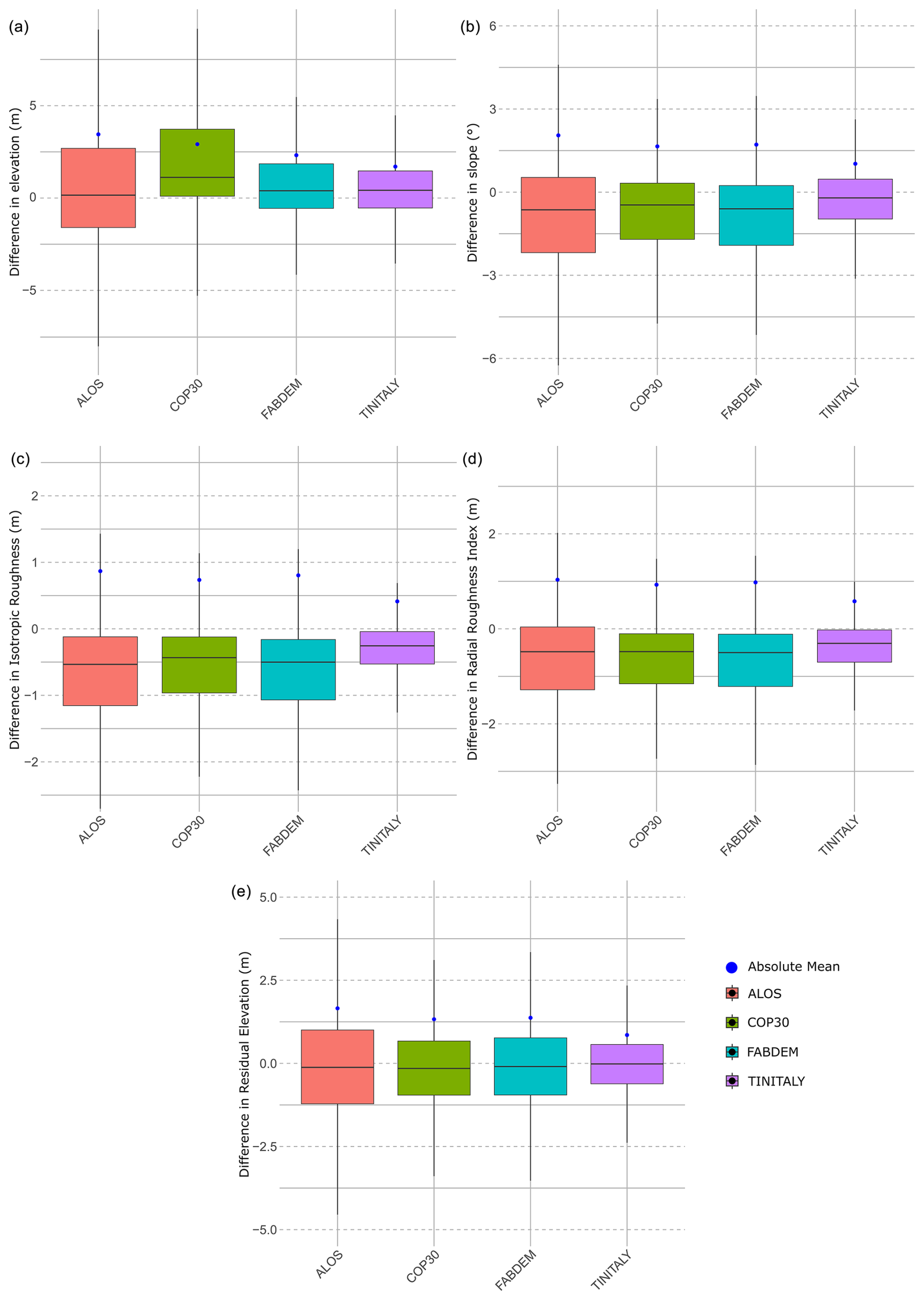
Figure 3 Boxplots visualizing the differences among the DEMs at 30 m, using different metrics with the absolute mean calculated. (a) Elevation, (b) slope, (c) isotropic roughness index, (d) radial roughness index, and (e) residual DEM.

Overall, TINITALY resampled at 30 m (TINITALY30m) shows the best performance across all metrics, with a smaller distribution of differences and a lower absolute mean difference. ALOS, on the other hand, displays the largest difference among all DEMs across all metrics. Between COP and FABDEM, COP shows a larger distribution of elevation differences, and, as expected, COP has a stronger tendency to overestimate elevation with respect to FABDEM (Fig. 3). However, for slope (Fig. 3b) and isotropic roughness (Fig. 3c), FABDEM displays more spread in differences.

Figure 4 exhibits the differences in the selected derivatives between TINITALY30m and TINITALY10m. Apart from elevation, TINITALY at 10 m quantifies a larger distribution in normalized differences for the terrain indices. The absolute mean difference confirms this trend.

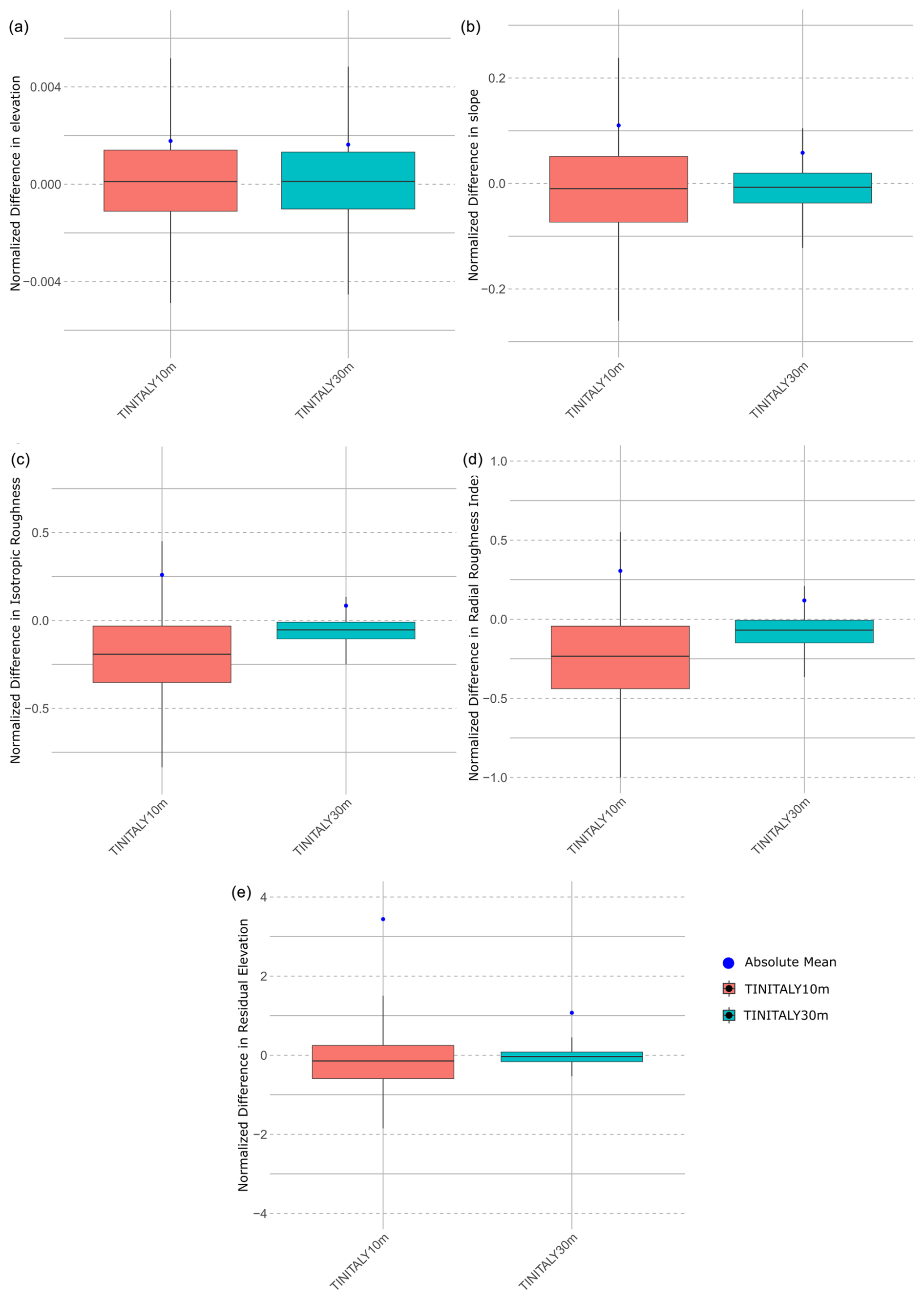
Figure 4 Boxplots showing the differences in TINITALY at 10 and 30 m with respect to the reference lidar at the respective resolution, for different indices with the absolute mean calculated. (a) Elevation, (b) slope, (c) isotropic roughness index, (d) radial roughness index, and (e) residual DEM.

Since the main topic of our analysis is to support landslide susceptibility mapping, we investigated the performance of the selected DEMs to derive slope, which is considered to be one of the most relevant landslide-predisposing factors, in the area where landslide bodies have been mapped. Figure 5 shows the slope difference within the mapped polygons of the PAI landslide inventory. TINITALY30m is seen to have the smallest differences in terms of absolute mean and distribution compared to all the other DEMs (Fig. 5a). Similarly, in Fig. 5b, the distributions of the normalized differences in TINITALY at 10 and 30 m clearly highlight the larger difference distribution of the 10 m DEM.

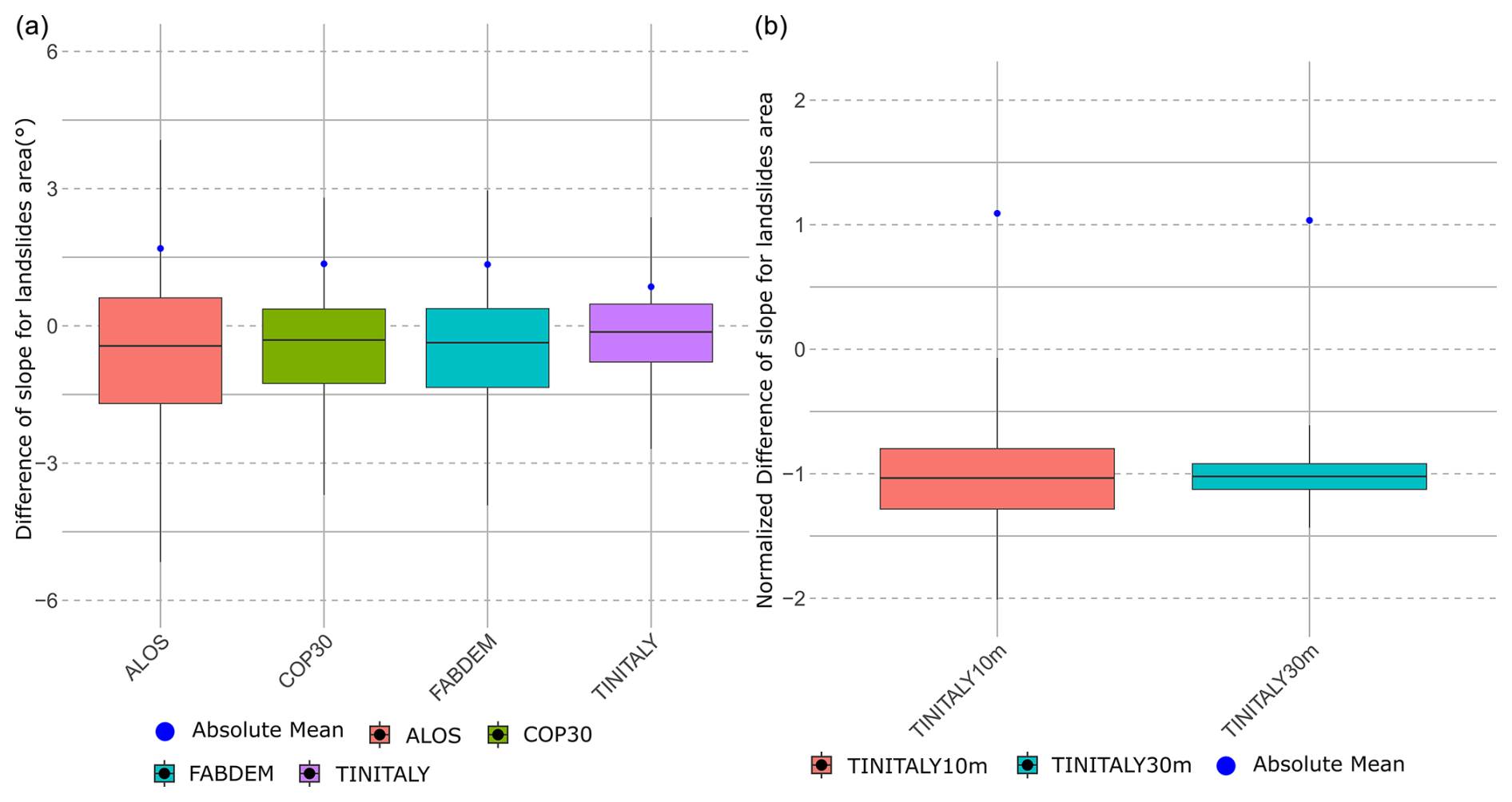
Figure 5 (a) Slope differences for 30 m DEMs as compared to the reference DEM in PAI landslide polygons. (b) Normalized difference in slope with reference DEM for 10 and 30 m TINITALY in PAI landslide polygons.

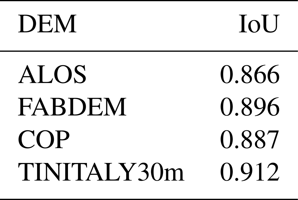
The last part of the DEM comparison investigates the effect on the SU delineation of different DEMs. Table 1 reports the Jaccard index tested by comparing the SUs delineated with DEMs at 30 m with those generated with the reference DEM. The highest similarity index is for TINITALY30m.

Table 1 Jaccard index represented as intersection-over-union for SUs generated from the DEMs under analysis and the reference lidar DEM SUs.

The second phase of the analysis focused on optimal SU delineation to assess landslide susceptibility in AOIa. Since TINITALY30m was found as being the most accurate DEM to represent the morphology of the mountainous area of the Marche region in the previous analysis, we generated 18 SU combinations based on TINITALY30m to find the optimal SU partition of AOIa. Figure 6 shows the visual differences in delineation for some of the parameter combinations. Smaller values of circular variance and minimum area result in smaller dimensions of SUs, which can restrict heterogeneity between adjacent SUs. However, ideally, SUs should maintain external heterogeneity for better terrain representation.

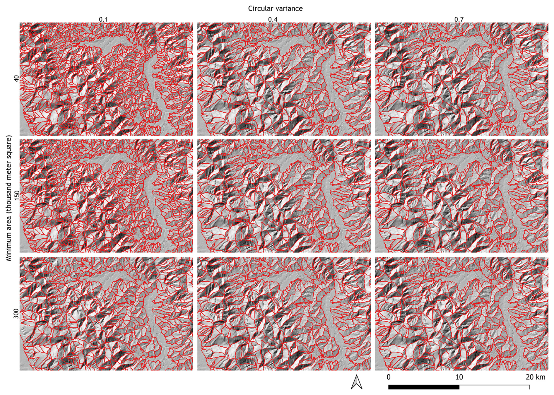
Figure 6 SU combinations. A total of 9 out of the 18 combinations are shown to highlight the differences as the values of two parameters change, i.e., minimum area and circular variance.

Figure 7 reports the behavior of the F, A, and D metrics and the final S metric based on the 18 combinations of a and c. Considering that each of the metrics represents a goodness of fit for the final SU partition, the higher the F, A, and D, the better the SU partition, excluding F, which shows an almost irregular pattern with the maximum at c equal to 0.1 and a equal to 40×10³ m² (Fig. 7.1). A and D have a mutually opposite, almost linear pattern, which reaches a maximum pairing: in A, where c is equal to 0.7 and a is each of the values assigned (Fig. 7.2), and in D, with c equal to 0.1 and a equal to 40×10³ m² (Fig. 7.3). A shows better performance, increasing the mapping unit extension of the study area, whereas D shows better performance with smaller partitions.

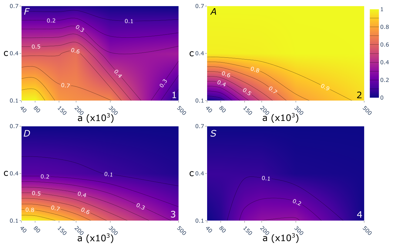
Figure 7 The behavior of the F, A, and D metrics and the final S metric with respect to parameters a and c: (1) shows the F value of the SU aspect segmentation metric, (2) visualizes the landslide extension inside a SU (A), (3) shows the landslide density (D), and (4) depicts the results of the final combined metric S.

The product of the normalized metrics results in the S value, which is maximized in the range of a between 300×10³ and 200×10³ m² and by a value of 0.1 for c (Fig. 7.4). Therefore, among the tested combinations, c equal to 0.1 and a equal to 300×10³ m² produce the optimal SU partition for landslide susceptibility mapping in the Marche region with an SU extension of 0.40 km² on average (dataset freely available on Ahmed and Titti, 2024). In contrast, the worst-case partition is the one which combines c equal to 150×10³ m² and a equal to 0.7 with an SU extension of 0.84 km² on average.

Consequently, a susceptibility assessment with the S optimal- and worst-case SU partition was carried out. The maps resulting from the susceptibility analysis and the relative confusion matrixes based on the S optimal- and worst-case SU delineation of the TINITALY30m dataset are represented in Fig. 8, while the quality metrics generated from the 10-fold spatial cross validation by ROC analysis are reported in Fig. 9. The summary of these metrics is provided in Table 2.

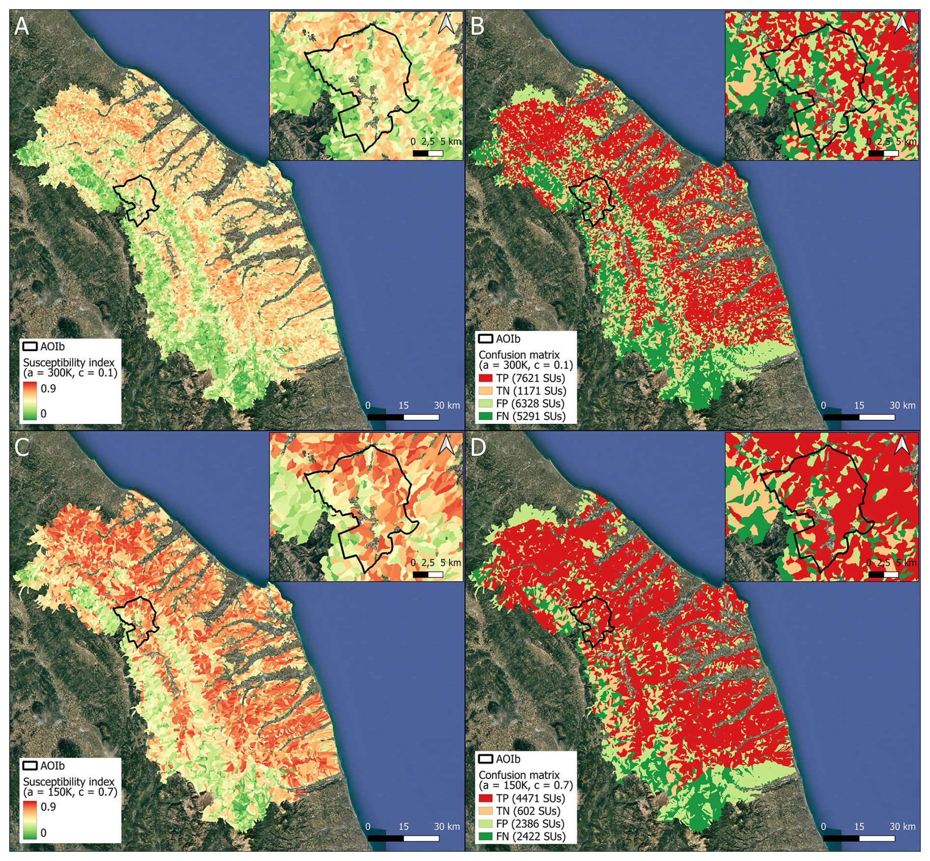
Figure 8 Landslide susceptibility mapping with TINITALY30m using (a) the selected optimal SU delineation ($a=\mathrm{300}\times {\mathrm{10}}^{\mathrm{3}}$ m², c=0.1) with the relative confusion matrix (b) (TN 6 % of all units and 13 % of unstable units) and (c) the selected worst-case SU delineation ($a=\mathrm{150}\times {\mathrm{10}}^{\mathrm{3}}$ m², c=0.7) with the relative confusion matrix (d) (TN 6 % of all units and 12 % of unstable units). The image background is from © Google Maps 2019.

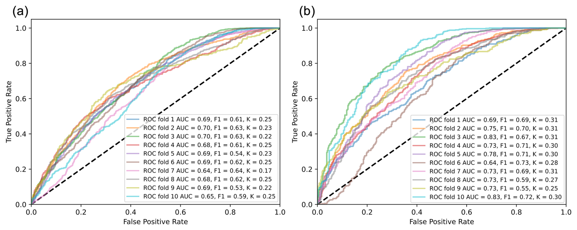
Figure 9 ROC curve with AUC, F1 score, and Kappa coefficient values for 10-fold cross validation. (a) The optimal SU delineation ($a=\mathrm{300}\times {\mathrm{10}}^{\mathrm{3}}$ m², c=0.1); (b) the worst-case SU delineation ($a=\mathrm{150}\times {\mathrm{10}}^{\mathrm{3}}$ m², c=0.7).

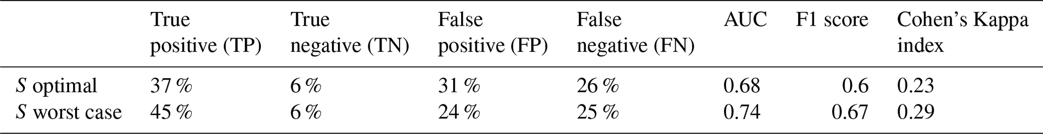
Table 2 Summary of confusion matrix from maps in Fig. 8 and performance metrics in Fig. 9.

In addition, two more landslide susceptibility analyses were carried out using SU partitions with intermediate S values – c equal to 200×10³ m² with a equal to 0.4 and c equal to 40×10³ m² with a equal to 0.1 – to investigate the relation between AUC and the number, or extension, of the slope units (see Sect. 5).

5 Discussion

Based on the results of the quantitative comparison between ALOS, COP, FABDEM, TINITALY10m, and TINITALY30m, the latter performed better than the other DEMs as per the indices used in this study (Fig. 3). These comparisons are insightful with respect to morphological differences. For instance, in terms of roughness indices (Fig. 3d), all DEMs tend to oversmooth compared with the reference DEM. This can be indicative of the spatial support being larger than 30 m in reality, meaning that the spatial data density is much lower than the given resolution. It is also interesting to note the difference between COP and FABDEM. FABDEM (DTM), being a product of COP (DSM), should in essence be closer to the lidar representation of the terrain with vegetation and buildings removed, but it produces a less accurate output. The efforts to generate a DTM from COP have been motivated by the application of flood modeling, aiming to optimize terrain representation, especially in areas of relatively low elevation. However, the algorithm has not been devised for optimizing geomorphometric derivatives such as slope (Hawker et al., 2022). This can be particularly relevant when modeling slope instability. Thus, FABDEM in the region considered does not improve the terrain representation as compared to COP (Bielski et al., 2024). This behavior is visible in Fig. 3, where FABDEM shows larger difference distributions than COP for slope, residual DEM, and both roughness indices. For instance, with regard to roughness indices (Fig. 3d), all DEMs tend to oversmooth compared to the reference DEM, which can be indicative of the spatial support being larger than 30 m in reality, meaning that the spatial data density is much lower than the given resolution.

ALOS consistently features large differences in all computed metrics against the other global DEMs, which could be explained with the analysis of Caglar et al. (2018). They concluded that ALOS contains a significant number of anomalies in elevation values, possibly attributed to unfiltered sensor noise and processing algorithms, which are often not easily identifiable. Nonetheless, ALOS still ranks well above other global products, like SRTM and NASADEM, according to quantitative assessments on DEM-derived parameters and is still comparable with COP and FABDEM (Bielski et al., 2024; Guth et al., 2024).

The numerical comparisons resulting in Fig. 3 can be supported by the graphical representation of the slope differences in Fig. 10. Although the spatial distribution of differences varies, larger differences are most noticeable in the ALOS DEM, followed by COP and FABDEM, compared to TINITALY30m, which exhibits fewer differences in slope compared to the reference DEM.

TINITALY was originally published with a pixel size of 10 m×10 m. Since the pixel sizes of the open global DEMs selected to be compared with the reference DEM in AOIb are around 30 m×30 m, we decided to conduct the entire analysis using the same grid cell size of 30 m. Therefore, the original TINITALY10m was resampled to a 30 m×30 m cell size. Despite this, the accuracy of TINITALY10m was also investigated, during which we compared the performance of TINITALY30m and TINITALY10m using normalized differences instead of simple differences. Although this was not the primary aim of the study, the tests indicate that TINITALY at 30 m pixel size outperforms TINITALY at 10 m pixel size (Fig. 4). These differences in performance, apart from the expected lower uncertainty related to the larger spatial support, may be attributed to the interpolation approach used for TINITALY10m. In areas with low sampling density, noticeable artifacts appear, which can significantly affect the calculation of geomorphometric derivatives. Resampling from the original 10 m pixel size to a coarser one (30 m) can partially filter out these artifacts. Thus, higher resolution does not necessarily guarantee better results if it is not supported by high-quality elevation data or if it contains a high number of artifacts (Chen et al., 2020; Mahalingam and Olsen, 2016). Additionally, the use of contour lines as input data for TINITALY10m along with a triangulator for interpolation may result in spurious spikes at regular intervals within elevation zones and in areas with triangular slope faces (Zingaro et al., 2021). Considering the acquisition dates of DEMs in comparison to the lidar, COP and ALOS were surveyed closer to the time of the lidar than TINITALY, but even so, TINITALY30m showed better results when compared with the lidar. Comparing slope differences in landslide areas across the selected global open-access DEMs, as well as TINITALY10m and TINITALY30m, yields similar results. The graphs in Fig. 5 present a distribution of relative differences similar to those in Figs. 3 and 4.

The similarity between the geometry of delineated SUs with the same parameters, as compared with the ones delineated from the reference DEM, indicates a higher value of the Jaccard index for TINITALY30m. This means that the SUs delineated using TINITALY30m most closely resemble those from the reference lidar DEM. The remaining global DEMs also produce SUs with a high similarity index.

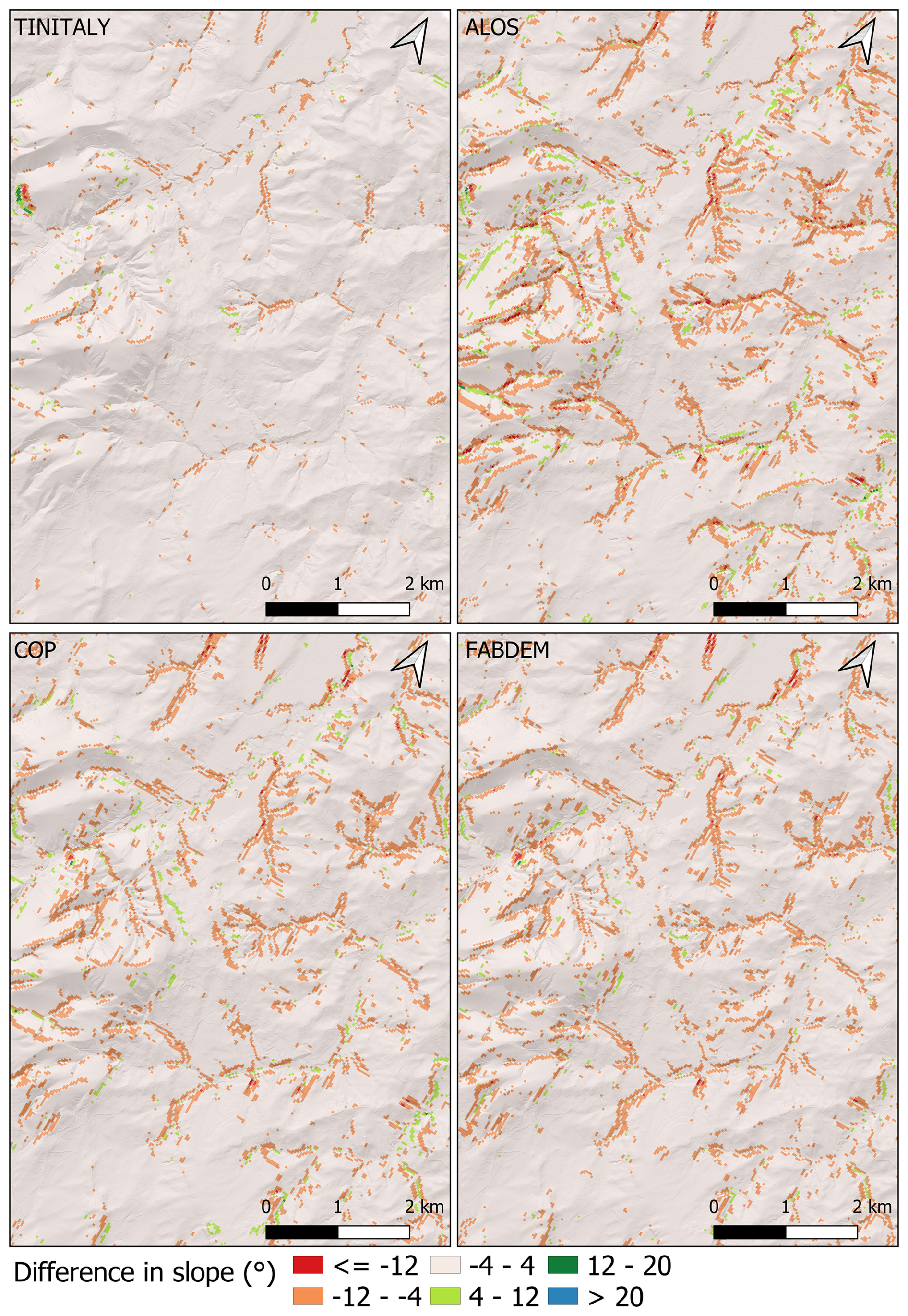
Figure 10 Difference in slope (degrees) between the four tested DEMs (30 m) and the reference lidar DEM, by subtracting the lidar value from the test DEM value.

In the end of phase 1, we can conclude that for the Marche region, the use of the 30 m resampled TINITALY DEM is recommended for SU definition; therefore the rest of the analysis proposed for phase 2 was based on TINITALY30m.

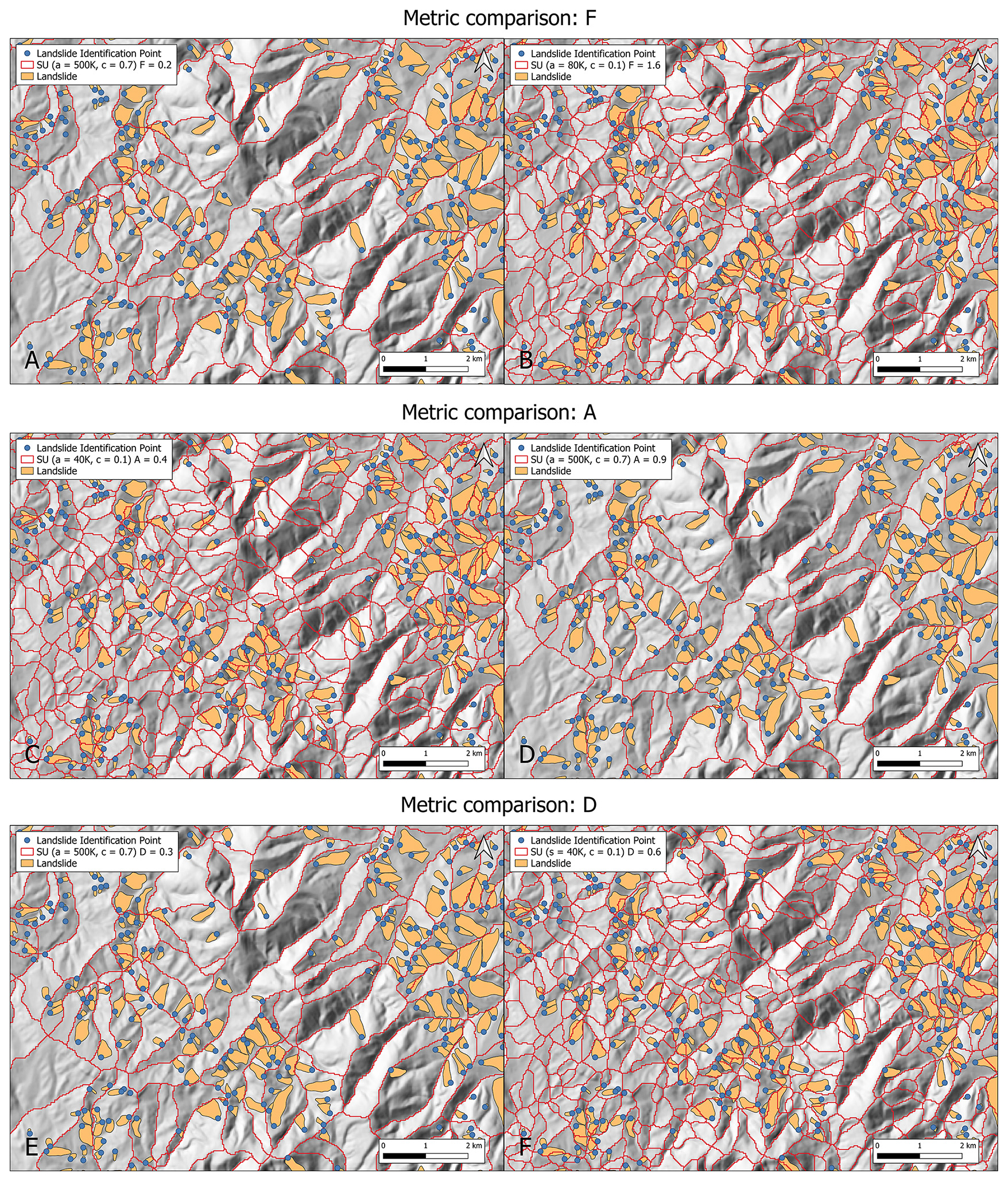
Figure 11 Selection of SU partition of a sub-portion of the study area AOIa. (a, b) The SU partitions with the lowest and the highest value of F, respectively; (c, d) the SU partitions with the lowest and the highest value of A, respectively; and (e, f) the SU partitions with the lowest and the highest value of D, respectively.

Extending the analysis of SU delineation from AOIb, we used multiple SU parameters for a more detailed analysis in AOIa with landslide polygons. Understandably, slope-facing direction and slope angle can be regarded as driving factors for slope failures and can be used to divide the terrain into units that can morphologically describe landslide-prone areas. Landslide susceptibility evaluates the probability of occurrence of a landslide according to a set of variables. Susceptibility depends upon a set of variables whose values are associated in a unitary manner with each mapping unit. Therefore, the mapping unit represents a portion of territory that each variable describes numerically by a single value as if it were a point object. Consequently, the smaller the dimension of the mapping unit, the more representative the single variable is. However, a spatial event such as a landslide, which is a non-point event, does not represent a homogeneous object according to the variables chosen to predict it (i.e., the degree of slope is not homogeneous throughout the landslide area). Thus, to evaluate the probability of occurrence of this event, it is necessary to identify unique values for each chosen predictor calculated within a portion of territory that coincides as much as possible with the landslide. It is also comprehensible that including stable areas, the portion of territory that most closely resembles the landslide area is the slope aspect, which can be represented by the SU. Therefore, to satisfy both of the requirements described above, the mapping unit should be as concise as possible to describe the shape of the landslide area.

The methodology adopted to evaluate the SU subdivision was designed to address the aforementioned requirements by integrating new metrics specifically tailored for landslide studies, considering the relevance of terrain units to landslide inventories. In addition to the aspect segmentation metric (F) proposed by Alvioli et al. (2016), the landslide extension coefficient (A) and the landslide density coefficient (D) have also been included. In a way, the F metric can define the shape of the SU on the basis of the spatial aspect distribution (Fig. 11a and b), while a balance between A and D can define the extension of the SU.

According to A, the optimal SUs are those that contain the entire landslide, with no landslide area falling into adjacent SUs. The landslide coefficient A may not fully capture the extent of landslide area, especially when dealing with landslides characterized by high mobility, as in the case of flow-like landslides, which can reach considerable distances where the run-out may move beyond the homogenous slope aspect. Nevertheless, the frequency distribution of the landslide classes in the landslide inventory will balance the A value, therefore the run-out of flow-like landslides may have an impact on the SU dimensions if their presence is significant in the inventory. Otherwise, part of the unstable area may fall into the adjacent SUs. Consequently, the larger the SU, the higher the probability of including the entire landslide, as is visible in Fig. 11c and d, where an example of the lowest- and highest-performing SU partition according to A is represented. In contrast to A, the D metric would avoid the overestimation of the SU dimension, which should be limited, ideally, to a single landslide (see the example in Fig. 11e and f). The correct use of the D metric requires that reactivated landslides should be excluded and regarded as unique events to avoid doubling the number of polygons in the same spatial unit.

The variability of the SU extension with respect to the parameters a and c can also be described through the number of unstable units in relation to the total number of SUs. Figure 12 shows that as D increases and A decreases, the unstable units increase. As D increases and A decreases, the SU extension is reduced, and therefore SU count increases.

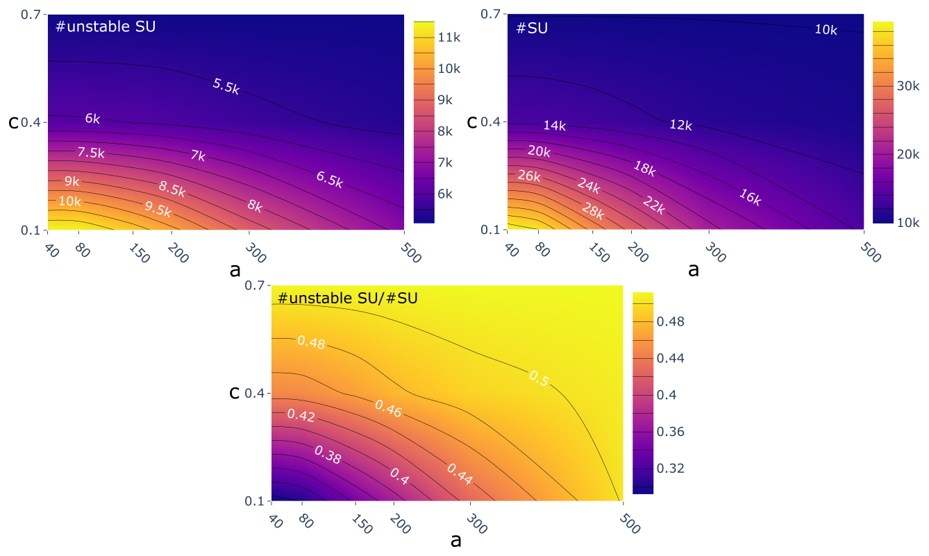
Figure 12 Evolution of the portion of unstable SUs in the study area with varying values of a and c.

All metrics unified in S maximize their effect, as shown in an example in Fig. 13, where the comparable differences explain the concept of the relation between the number and extent of landslides contained in the SUs. While it is difficult to minimize SU area and contain the landslide area, it should be considered that the spatial and areal accuracy of landslide inventories can significantly affect the output since the best terrain partition is interpreted based on the dimensions and number of landslide polygons. In this case study, the PAI of the Marche region was used to test the methodology, and while the landslide inventory plays a crucial role, it has to be mentioned that the dataset used may come with limitations. The inventory has not been systematically updated for the mapped landslide areas, and the dataset has been updated using reports from scientific literature, local authorities, and projects of the municipalities (Costanzo and Irigaray, 2020). Nonetheless, the methodology remains compatible with landslide polygons and SUs, supporting the selection of an optimal terrain partitioning.

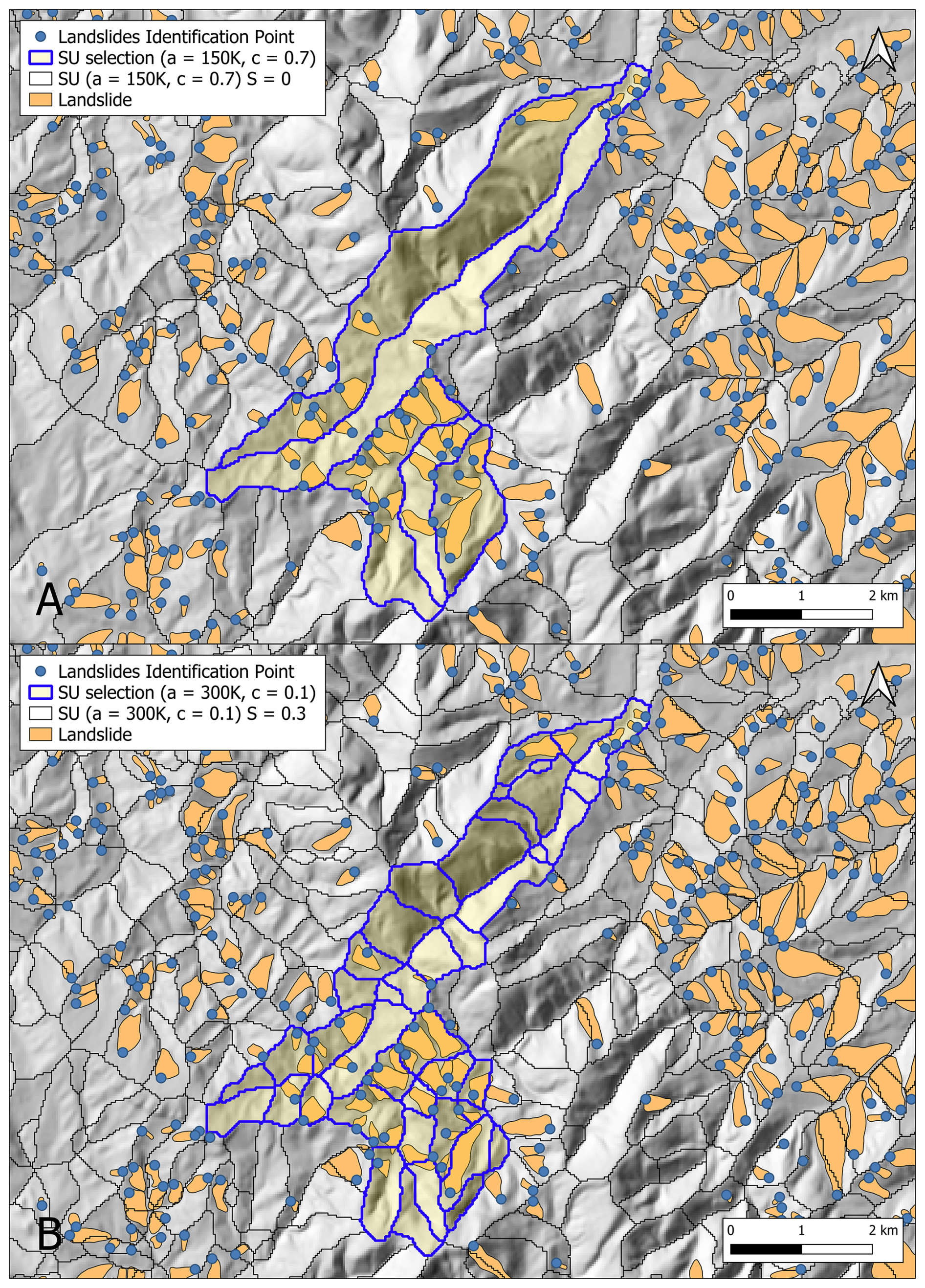
Figure 13 SU partitions of a sub-portion of the Marche study area (AOIa) compared to landslide distribution from the PAI. (a) The SU partition ($a:\mathrm{150}\times {\mathrm{10}}^{\mathrm{3}}$ m² and c:0.7) with the lowest value of S and (b) the SU partition ($a:\mathrm{300}\times {\mathrm{10}}^{\mathrm{3}}$ m² and c:0.1) with the highest value of S.

Two susceptibility analyses have been carried out by selecting the S optimal- and worst-case SU partitions. Since the goal of this study is not to assess landslide susceptibility of the Marche region but to investigate the potential effect of a thought-out SU delineation for landslide susceptibility evaluated with largely used metrics such as AUC, F1 score, and Cohen's Kappa score, the predisposing factors selected for the susceptibility analysis are not entirely representative of the geo-environmental conditions. In particular, not all predisposing factors (e.g., land use and vegetation indices) have been considered (see also Titti et al., 2024). Therefore, the cross-validation results (Fig. 9a) of the susceptibility map (Fig. 8a) calculated with the optimal SU subdivision do not perform well in the metrics considered (AUC=0.68, F1 score=0.6, K=0.23 on average). Nevertheless, it is interesting to highlight the trend of the relation between the mapping unit extension and the AUC value along with other metrics.

AUC is calculated as the integral of the ROC curve. The ROC curve depends on the balance between unstable units and stable units in the training dataset. Thus, the higher the ratio between the number of unstable SUs and the total number of SUs, the higher the AUC because the model's ability to recognize true positive (TP) mapping units increases, thereby increasing the true positive rate (TPR) of the ROC curve. In the 18 combinations selected to investigate the highest-performing a and c values for SU delineation, we did not change the landslide number but rather the extension of the SUs whose trend is visible through the number of SU patterns in Fig. 14. Considering all the combinations of a and c performed in our experiment, the higher the extension of the mapping units, the higher the proportion between the number of unstable units and the number of all the mapping units and the higher the AUC (Fig. 14). The same considerations can be made for the F1 score and Cohen's Kappa index, whose behavior follows a similar trend to that of the AUC.

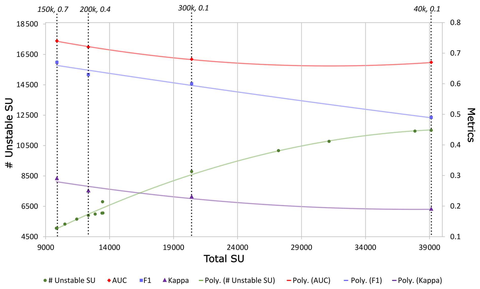
Figure 14 Trend in the number of unstable SUs and total SUs (of 18 combinations for a and c) and the behavior of the metrics resulting from the landslide susceptibility analysis. The parameters (a, c) are labeled along the performance metrics to represent the respective trend.

Therefore, at least in the experiments carried out for this study, the metrics selected are not suitable for comparing susceptibility maps directly because the training datasets are differently balanced. Nevertheless, a comparison between the S optimal- and S worst-case susceptibility maps, as shown in Fig. 8a and c, respectively, can still be made. Graphically, the maps exhibit a similar spatial pattern of landslide probability of occurrence. This is further supported by the fact that the number of TN units relative to unstable units is nearly the same, at 13 % and 12 % for the S optimal- and the S worst-case scenarios, respectively. The primary distinction lies in the susceptibility value, which is on average lower in the S optimal-case delineation than in the S worst-case delineation. This difference is attributed to the overestimation of unstable units in the S worst-case scenario due to the imbalance between stable and unstable units.

6 Conclusions

This study encompasses DEM utilization from the viewpoint of fine-scale morphology and terrain subdivision into mapping units in the framework of regional predictive landslide modeling. The aim is to compare freely available global and national DEMs, from which morphological landslide-predisposing factors and optimized terrain partition into slope units are derived to map landslide susceptibility. Therefore, the investigation initially identified the optimal DEM among those available and then selected the optimal SU partition in the alternative combinations generated.

The global DEMs (ALOS, COP, FABDEM) and TINITALY resampled at 30 m have shown considerable differences compared to the reference DEM (an airborne lidar resampled at a 30 m pixel size) in the selected geomorphometric derivatives in AOIb. Concerning the SU delineation, TINITALY30m has shown the best performance; thus, it was selected to generate 18-parameter SU subdivisions in AOIa. To define the optimal SU delineation, a novel method has been proposed, which evaluates SU alternatives based on internal aspect homogeneity/external heterogeneity, the number of landslides, and landslide extension. According to the S metric (Eq. 6), the SU partition generated with c equal to 0.1 and a equal to 300×10³ m² results in the optimal subdivision, contrasting with c equal to 0.7 and a equal to 150×10³ m² as the worst-case subdivision.

Ultimately, to understand the effect of the terrain partition on the landslide susceptibility model, we performed the S optimal- and the S worst-case landslide susceptibility. It is understood that the performance metrics (AUC, F1, K) of the landslide susceptibility models do not necessarily equate with the S metric performance. Indeed, AUC, F1, and K depict opposite trends to those of the S metric.

Although only TINITALY30m was used to extend the analysis for SU experiments, COP, as the second-best-performing DEM for fine-scale morphology, can also be considered in future studies. A holistic comparison could help evaluate its effectiveness in landslide susceptibility studies. Moreover, since the result of the S method depends on the landslide inventory, further research could pave the way for space–time inventories that perform multi-temporal SU delineations to reach the best terrain delineation for slope failure prediction. Developing space–time landslide inventories and adapting SU delineation for dynamic, evolving terrains could significantly enhance the predictive capability of landslide models. Ultimately, continued innovation in DEM selection, SU partitioning methods, and landslide inventory development will contribute to more effective landslide risk management strategies and mitigation efforts.