Simulation analysis of 3D stability of a landslide with a locking segment: a case study of the Tizicao landslide in Maoxian County, southwest China

Rock bridges, also known as locking masses in landslides, affect the three-dimensional (3D) stability and deformation patterns of landslides. However, it is always difficult to simulate rock bridges with continuous grid models in 3D landslides due to their discontinuous deformations. Tizicao landslide, located in Maoxian County, southwest China, is a typical landslide with a super-large rock mass volume of about 1388.2 × 10⁴ m³ and a locking segment. To explore a better rock bridge model used to simulate 3D stability and deformations of the Tizicao landslide, this study introduced three rock bridge models into the FLAC3D program, including the intact rock mass model (IRMM), the Jennings model (JM), and the contact surface model with high strength parameters (CSM-HSP). The CSM-HSP model was eventually used in the FLAC3D program to obtain the 3D deformation characteristics of the landslide. In addition, the two-dimensional (2D) stability of the Tizicao landslide was analyzed using the GeoStudio program. The simulation results indicate that the Tizicao landslide is generally stable under current conditions owing to the existence of the locking segment in its southern front. This inference is consistent with the field deformation and monitoring data. It was found that the general stability and local deformations of the landslide are influenced by the locking segment according to the comparison between the 2D and 3D stability. There was a linear relationship between the locking ratio and the factor of safety (Fos), which applied to the 2D stability analysis of the landslides with a locking segment each, while there existed an approximate quadratic parabola suitable for the 3D stability of the landslides. Finally, this study analyzed the laws of the 3D Fos varying with the locking ratio and strength parameters of the locking masses and the sliding surface. Furthermore, it explored the advantages and disadvantages of the three rock bridge models in the simulation of the 3D stability of landslides with a locking segment.

1 Introduction

A landslide with a locking segment refers to a geological phenomenon in which a locking segment exists along the sliding surface of a landslide, and the critical failure of the landslide is controlled by the shear properties of the locking segment (Xu et al., 2010; Huang, 2012; Lin et al., 2018). A landslide of this type usually holds huge potential energy (Huang, 2012), which will be suddenly released once the locking masses of the landslide are cut off. As a result, a mass of fragmental materials from the landslide will affect the residential areas and infrastructure below the landslide, thus frequently resulting in catastrophic effects and heavy casualties (Yin et al., 2011; Lin et al., 2018; Wang et al., 2019). The analysis of locking masses is the key to the analysis of the stability of a landslide with a locking segment. However, the locking segment in the landslide is characterized by uncertain positions, irregular shapes, and varying curvatures, which make the analysis of the 2D stability of the landslide more difficult. Meanwhile, the 2D stability analysis is often applied to engineering reinforcement design and is relatively conservative, and the analytical results can represent only the local stability of a landslide (Li et al., 2010; Park and Michalowski, 2017). Therefore, 3D stability analysis plays a critical role in assessing and predicting the overall stability of the landslide with a locking segment.

At present, the commonly used methods for the 3D stability analysis of landslides include limit equilibrium and numerical simulation. Many 3D limit equilibrium methods have been proposed to account for the 3D stability of slopes (Hovland, 1977; Leshchinsky et al., 1986; Hungr et al., 1989; Lam and Fredlund, 1993). However, most of them are simply based on the extension of the 2D limit equilibrium slice methods proposed by Bishop (1955), Morgenstern and Price (1965), and Spencer (1967); thus the inherent limitations of the deformation and failure mode analysis remain. Fortunately, the simulation methods provide a simple and useful way of analyzing both the 3D stability and the deformation and failure tendency of landslides, and they have been employed to determine the 3D stability of slopes and landslides (Deng et al., 2011; Wang and Xu, 2013; Zhang et al., 2013; Ma et al., 2020). Nevertheless, the numerical simulations of the 3D stability analysis of landslides mostly ignore the rock bridge effect. As indicated by simulation studies of 2D or 3D planar stability, the stability and the failure mode of slopes and landslides with rock bridges are determined by their rock bridges (Stead et al., 2006; Huang et al., 2015; Glueer and Loew, 2015). In addition, several problems related to rock bridges are yet to be solved, including the response of the 3D stability of landslides to rock bridges, the controlling effects of rock bridges on slope deformation, and the simulation of rock bridges in numerical simulation software.

Some researchers have found that the stability of slopes and landslides with rock bridges is closely related to the length, penetration rate, strength parameters, joint strength parameters, relative positions (direction, coplane, or non-coplane), and shape of rock bridges (Einstein et al., 1983; Tuckey and Stead, 2016; Romer and Ferentinou, 2019; Zhang et al., 2020) and determined the qualitative relationships between the 2D stability of slopes and landslides and these parameters. However, there is a lack of in-depth quantitative study on these relationships, especially on the 3D stability of slopes and landslides.

The objective of this work is to present an improved rock bridge model and to simulate 3D stability and deformation behaviors of the Tizicao landslide using the model. Three rock bridge models, i.e., intact rock mass model (IRMM), Jennings model (JM), and contact surface model with high strength parameters (CSM-HSP), were introduced into the FLAC3D program in this study. Then, this study explored the advantages and disadvantages of the three rock bridge models in the simulation of the 3D stability of landslides with a locking segment through a comparative analysis. It also explored the effects of the locking masses on the 3D stability of the landslide by analyzing the laws of the 3D factor of safety (Fos) varying with the locking ratios and strength parameters of the locking masses and the sliding surface.

2 Study site

The Tizicao landslide is located in Maoxian County, Sichuan Province, southwest China (Fig. 1), with geographical coordinates of 31°53^′14.89^′′ N and 103°40^′51.12^′′ E. It lies on the right bank of the Minjiang River and faces the town of Shidaguan on the left bank of the river (Fig. 2a). The Tizicao landslide has a length of about 680 m, a width of 570 m (Fig. 2a), an average thickness of about 39.1 m, and a volume of 1388.2 × 10⁴ m³. This landslide has a huge gravitational potential energy due to the relative elevation difference of 220 m between the toe of the landslide and the lower riverside of the Minjiang River (Fig. 2a).

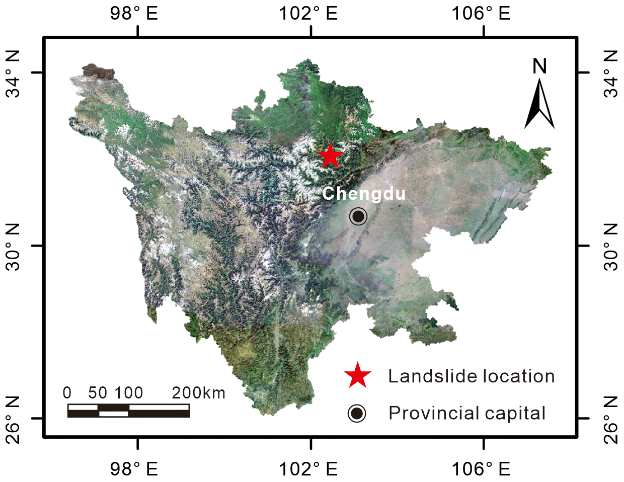
Figure 1 Location of the Tizicao landslide in Sichuan Province, southwest China. Source: © Google Earth Pro 2021.

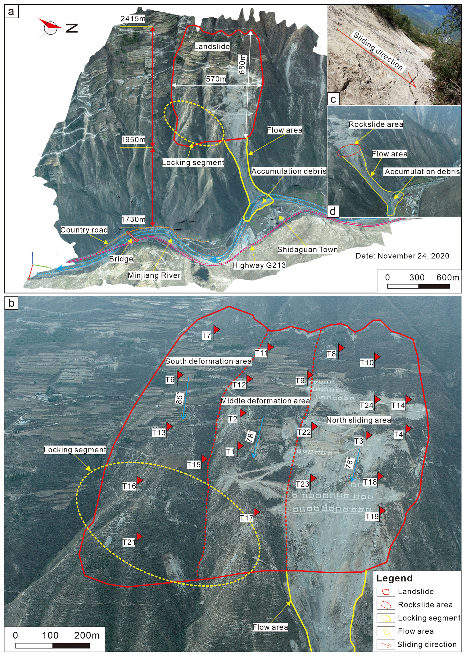
Figure 2 Overall perspective of the site area of the Tizicao landslide (after Zhou et al., 2022). (a) An orthoimage of the landslide site area taken on 24 November 2020, with a resolution of 3840 × 2160. (b) Three deformation areas of the Tizicao landslide. The dashed red line denotes the boundary of the deformation area. The red flag denotes the location of the 24 fixed non-prism monitoring points (T1–T24). (c) Rear wall. (d) Rockslide area, flow area, and accumulated debris.

Moderately high mountains and river valleys occur in the area of the Tizicao landslide. This area is largely a part of Minshan Mountain of the Qionglai Mountains, and its southeastern boundary belongs to the final segment of the Longmen Mountains (Wang et al., 2019). Moreover, this area exhibits steep and dangerous valleys and slopes, narrow river valleys, and deeply downcutting rivers. The Minjiang River flows through this area in a nearly north–east direction. The main body of the Tizicao landslide consists primarily of silty clay ($Q_{\mathrm{4}}^{\mathrm{del}}$) on the surface and broken phyllite below, and its sliding bed mainly comprises weak and broken carbonaceous phyllite of the Devonian Weiguan Group (Dwg²), which has poor physical and mechanical properties and poses risks of failure, sliding, and deformation during rainy seasons.

According to the field survey by Zhou et al. (2022), the middle-front part of the Tizicao landslide began to deform in 2013, when the houses on the slope started to crack and dislocate downward. In September 2014, the middle part of the landslide's front gradually collapsed. As a result, a flow area with a width of about 60 m and a height of 200 m (Fig. 2d) was formed. As a result, the accumulation body fell into the Minjiang River, forming a landslide dam. Meanwhile, the landslide's rear (Fig. 2c) began to crack. From August to September 2015, the landslide deformed more apparently and severely, resulting in additional wide and long cracks. After continuous deformations during the rainy season in 2016–2017, the rear and front of the landslide had dislocated downward for more than 10 m locally by July 2017. The collapse with a volume of about 6.0 × 10⁴ m³ occurred in the northern front of the landslide body, blocking the Minjiang River for several hours. Fortunately, no casualties occurred. Since October 2017, the deformation of the landslide has slowed down and tended to stabilize (Fig. 3c). However, once a large-scale slide occurs, this landslide would directly threaten the lives of 30 people on the slope body, even seriously threatening the lives of 113 people in Shidaguan (Fig. 2a) below the landslide. Moreover, more than 30 buildings and a 2 km long section of the National Highway G213 will also be destroyed.

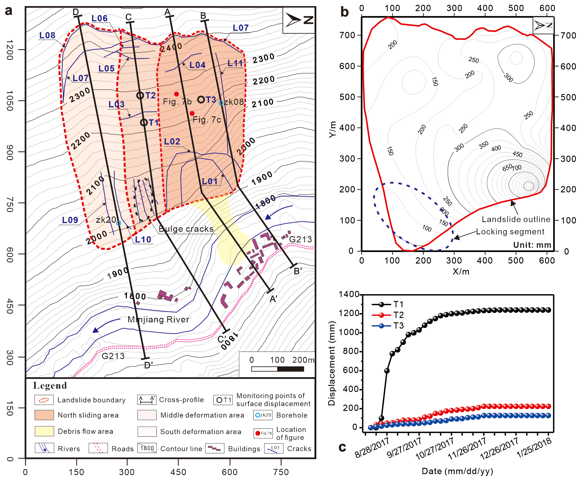
Figure 3 The topographic plan, isoline map of surface displacement, and displacement monitoring curves of the Tizicao landslide. (a) Topographic plan of the deformation areas, the crack distribution, and the locations of geotechnical-engineering sections (after Zhou et al., 2022). (b) Isoline map of the surface displacement of the Tizicao landslide from 13 August 2017 to 25 January 2018 (Zhou et al., 2022). (c) Displacement monitoring curves of the landslide surface (from 13 August 2017 to 25 January 2018).

Monitoring was conducted using a Leica monitoring total station (TM50), which was set up on the slope opposite the landslide. In the landslide body, 24 fixed non-prism monitoring points (T1–T24; Fig. 2b), which almost covered the entire landslide body, were deployed to primarily monitor the surface displacement from 1 June to 2 October 2017. The raw data of the surface displacement were processed using the measurement adjustment software DDM to obtain the deformation amount, deformation rate, and isoline map of the surface displacement of the Tizicao landslide (Fig. 3b).

The Tizicao landslide can be divided into three areas according to the aerial photographs obtained using high-performance uncrewed aerial vehicles, field surveys, and monitored deformation data (Figs. 2b and 3a).

The first is the north sliding area. This area is rectangular and covers an area of 11.15 × 10⁴ m². It has a longitudinal length of 600 m, a transverse width of 258 m, and a sliding direction of 78°. A notable sliding failure has occurred in this area, as shown in Fig. 4a. Specifically, significant tensional deformations are visible at the landslide's rear in this area, forming a rear wall with a height of about 10 m (Fig. 2c). Moreover, a deep and large tension crack (crack L04; Fig. 3a) and a pinnate shear crack (crack L11; Fig. 3a) have developed in the middle part of this area. All these contribute to a sliding displacement of about 10.5 m overall in this area. The slope in the landslide's front is subjected to the most severe deformations. It has dislocated downward by up to more than 40 m, with about 6 × 10⁴ m³ of landslide masses having collapsed into the Minjiang River (Fig. 2d).

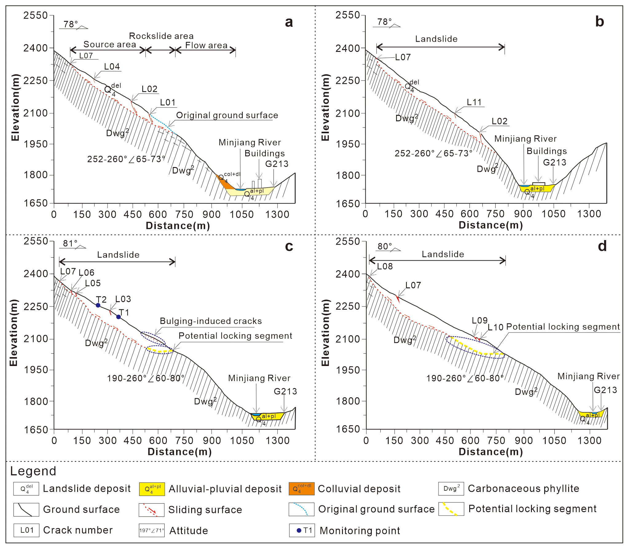
Figure 4 Geotechnical-engineering sections of the Tizicao landslide. (a) Section A-A'. (b) Section B-B'. (c) Section C-C'. (d) Section D-D' (after Zhou et al., 2022).

The second is the middle deformation area. This area is in the shape of a long strip and covers an area of 6.42 × 10⁴ m². It has a longitudinal length of 568 m, a transverse width of 138 m, and a sliding direction of 78°. As shown in Fig. 4c, the landslide's rear in this area exhibits severe deformations, forming a 5 m high rear wall (crack L07; Fig. 3a). Multistage cracking and depression deformations (cracks LF03, LF05, LF06, and LF07; Fig. 3a) have occurred in the middle part of the landslide in this area, with an overall displacement of about 8 m. Compression cracks and bulge-induced cracks (Fig. 3a) have formed in the landslide's front under the resistance of locking masses.

The third is the south deformation area. This area is in the shape of a long strip and covers an area of 13.21 × 10⁴ m². It has a longitudinal length of 700 m, a transverse width of 192 m, and a sliding direction of 85°. As shown in Fig. 4d, the landslide's rear in this area is controlled by cracks L07 and L08 and has dislocated downward by about 3 m. The displacement of the middle part of the landslide is about 1.5 m. The compression-induced longitudinal tension cracks (cracks L09 and L10; Fig. 3a) have mainly developed in the landslide's front in this area, while large-scale sliding has not occurred.

Zhou et al. (2022) identified and analyzed the locking segment of the Tizicao landslide. As indicated by their analytical results of the landform, spatial–temporal deformations, surface cracks, and rock quality in the landslide area, the locking segment of the Tizicao landslide lies at the south slope toe (Figs. 2a–b and 3b). The locking segment covers an area of about 4.69 × 10⁴ m², accounting for 15.2 % of the total area of the landslide. As shown in Fig. 4, the anti-dip carbonaceous phyllites of the Dwg² develop in the landslide area, and they exhibit different deformation characteristics in the locking segment and the non-locking segment subjected to landslide deformation and the unloading effect. For the locking segment in the landslide area, the surface layer consists of a loose accumulation body, which is composed primarily of grayish-yellow silty soil mixed with fragments and has a thickness of about 3–5 m. The lower sliding body consists of moderately to slightly weathered carbonaceous phyllites with attitudes of 190–260° ∠ 36–60° (Fig. 5a). The sliding bed is composed of the slightly weathered carbonaceous phyllites with attitudes of 190–260° ∠ 60–80°. The slightly weathered carbonaceous phyllites have straight and smooth bedding planes, without any fillings or with a small number of quartz veins with hard structural planes. These phyllites have a joint spacing of 0.05–1.2 m, and their rock masses have rock quality designation (RQD) values of 68.0 %–76.8 %. The anti-dip phyllites tend to deform along the slope direction, and the dip angles of their bedding planes decrease gradually with a decrease in the depth (Fig. 6). Furthermore, the anti-dip phyllites are less affected by landslide deformation with an increase in the depth. For example, the phyllites at a depth of 50 m in the drilling borehole (Fig. 6c) exhibit intact cores, a high-strength rock mass, and attitudes consistent with the slightly deformed anti-dip rock masses at the landslide's back (Fig. 5b). According to stereographic projections (Fig. 6d–f), the dip angle of the bedding plane and the stability of the landslide increase with an increase in the depth. Correspondingly, the anti-dip rock mass, which is similar to the rock bridge and is referred to as the locking segment herein, is the key block that prevents further landslide sliding. Only when the locking masses are cut off does the overall landslide failure occur.

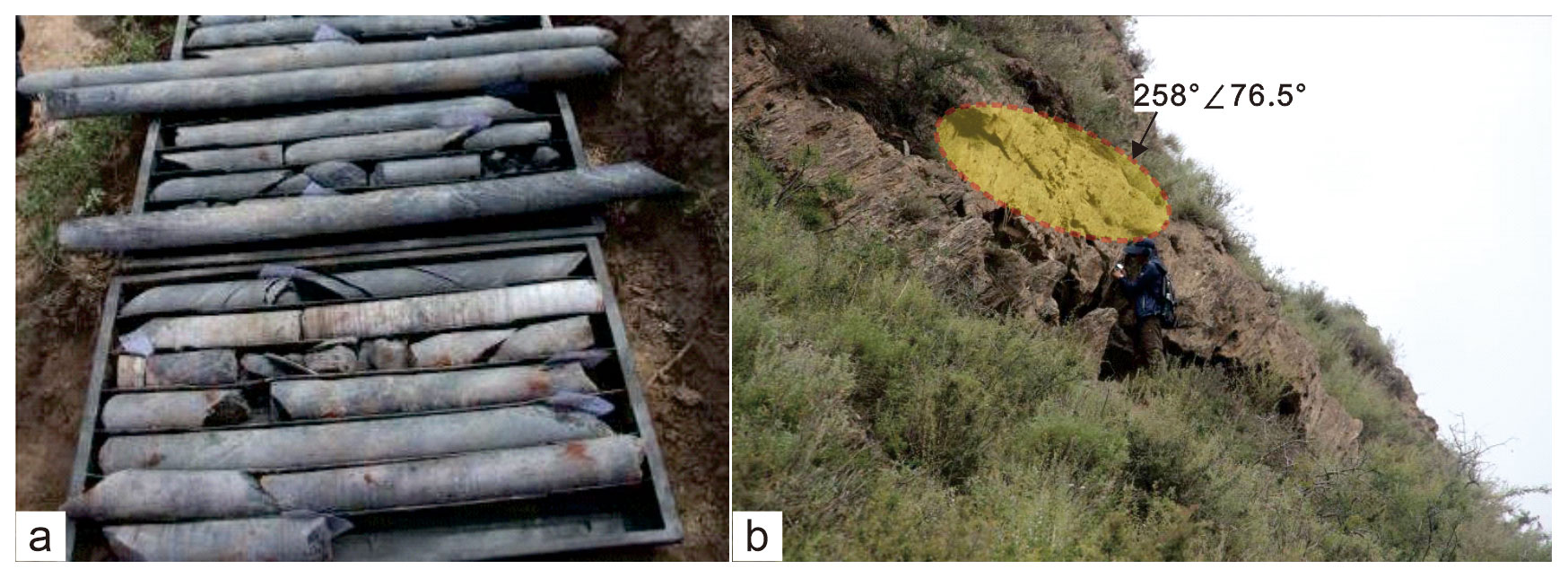
Figure 5 Rock cores drilled from borehole zk20 and exposed phyllites at the back of the landslide. (a) Intact rock cores (Zhou et al., 2022). (b) Exposed phyllites with an attitude of 258  76.5°.

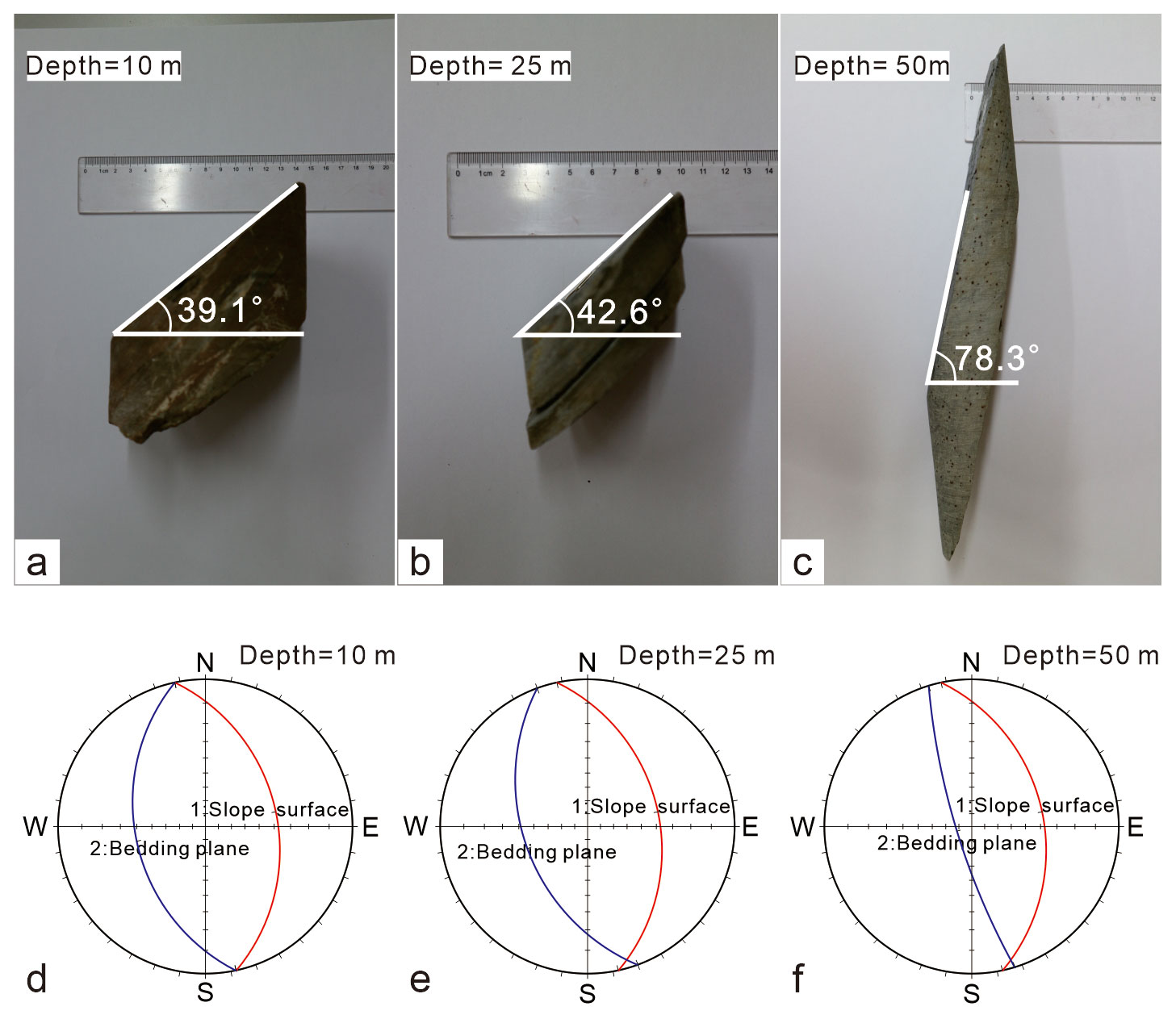
Figure 6 Rock cores and stereographic projections at different depths. (a–c) Rock cores at depths of 10, 25, and 50 m, respectively, in borehole zk20. The diameters of the drilling hole are 100 and 60 mm at the depths of 0–15 and 15–70 m, respectively. (d–f) Stereographic projections at the depths of 10, 25, and 50 m, respectively.

According to the discussion of Zhou et al. (2022), the locking masses of the Tizicao landslide occur on the convex bank, while the non-locking masses have developed on the concave bank, indicating that the locking masses are directly related to the S-shaped river valley under the landslide. From a geomorphological point of view, landslides rarely occur on convex banks but occur more frequently on concave banks. From a topographical perspective, a convex slope is more stable than a concave slope under the same conditions. Noticeably, the concave and convex banks of the S-shaped valley under the Tizicao landslide differ greatly in slope and lithology. Therefore, the rock masses on the south side of the landslide above the convex bank are intact and constitute the potential locking segment of the landslide.

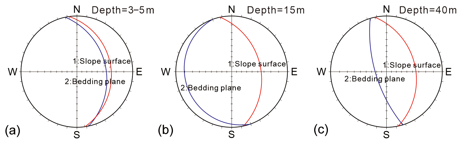
For the non-locking segment in the area of the Tizicao landslide, its surface layer is composed of grayish-yellow silty soil mixed with fractured rocks and with a thickness of about 6–8 m. Below the surface layer are the strongly weathered carbonaceous phyllites with a thickness of 25–33 m. The soils in the sliding zone can also be observed in the non-locking segment, with a thickness of about 0.5–1.2 m. Below the sliding zone are moderately weathered phyllites with attitudes of 252–260° ∠ 65–73°, joint space of 0.5–1.2 m, and RQD values of 15.0 %–54.5 %. Owing to the large deformation in the non-locking segment, the phyllites exhibit severe deformations, as manifested by the sliding of the phyllites along the slope direction after the stratum toppling (Figs. 7b–c, 8a). As shown in Fig. 8, the bedding planes of rock masses within the drilling depth (0–13 m) are along the slope direction, while the rock masses at a depth of more than 13 m are inclined in the opposite direction. The attitudes of rock masses below the sliding surface roughly remain unchanged. Therefore, the shear failure of the anti-dip phyllites is the fundamental cause of the large deformation in the north sliding area (Fig. 3a).

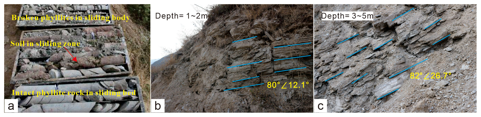
Figure 7 Rock cores drilled from borehole zk08 and extremely broken phyllites exposed due to construction excavation in the non-locking segment of the landslide. (a) Broken phyllites, soils in the sliding zone, and relatively intact phyllites in the sliding bed (Zhou et al., 2022). (b) Exposed phyllites with an attitude of 80° 12.1° at the depth of 1–2 m. (c) Exposed phyllites with an attitude of 82° 26.7° at the depth of 3–5 m. Cyan lines represent the bedding planes of the phyllites.

Figure 8 Stereographic projections at the depths of 3–5, 15, and 40 m (a–c, respectively).

3 Methodology

The 3D stability of the Tizicao landslide was simulated using the FLAC3D program. First, we introduced three rock bridge models, namely IRMM, JM, and CSM-HSP, into the FLAC3D program and determined the simulation elements and their characteristic parameters. According to the site survey of the Tizicao landslide, a 3D mesh model composed of a sliding bed, a sliding body, and a sliding surface was established. Then, we simulated the 3D stability of the Tizicao landslide using the three rock bridge models. Lastly, to compare the differences between the 2D and 3D stability of the Tizicao landslide, this study analyzed the 2D stability of four sections of the landslide using the SLOPE/W module of the GeoStudio 2012 program.

3.1 Rock bridge models in the simulation program

The FLAC3D program is used to simulate the 2D and 3D stability and deformation of landslides (Titti et al., 2020; Zhang et al., 2013; Zhou et al., 2020). To investigate the 3D stability and deformation behaviors of the Tizicao landslide, this study introduced three rock bridge models into the FLAC3D program, namely IRMM (Kemeny, 2005; Zhang et al., 2020), JM (Bonilla-Sierra et al., 2015; Jennings, 1970), and CSM-HSP (Huang et al., 2015; Scholtès and Donze, 2015), as shown in Fig. 9.

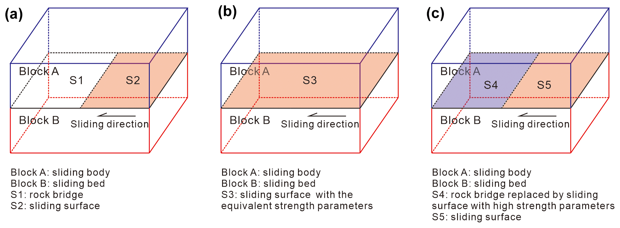
Figure 9 Three rock bridge models used in the FLAC3D program. (a) Intact rock mass model (IRMM). (b) Jennings model (JM). (c) Contact surface model with high strength parameters (CSM-HSP).

The IRMM model (Fig. 9a) is used to simulate the deformation and failure characteristics of rock bridges in rock masses. This model can effectively reveal the behaviors of stress concentration, cracking, extension, and penetration (Tang et al., 2001; Zhang et al., 2006). In the simulation of a landslide with a locking segment, the rock bridge (S1), which is an intact rock mass, was simulated using the tetrahedral elements in the FLAC3D program; the sliding surface (S2) was simulated using the contact surface model in the FLAC3D program; and the sliding body (Block A) and the sliding bed (Block B) were linked with the continuous rock bridge (S1).

For the JM model, the limit equilibrium method is initially employed to calculate the 2D stability of rock slopes with discontinuous joints. Specifically, the slope stability is calculated by assigning the equivalent shear strength corresponding to different penetration rates to the potential sliding surface. The equivalent shear strength parameters can be calculated as follows:

$$\begin{array}{}\text{(1)}& {\displaystyle }{c}_{\mathrm{eq}}=(\mathrm{1}-k)c_{\mathrm{r}}+k{c}_{\mathrm{j}},\text{(2)}& {\displaystyle }\tan {\mathit{\varphi }}_{\mathrm{eq}}=(\mathrm{1}-k)\tan {\mathit{\varphi }}_{\mathrm{r}}+k\tan {\mathit{\varphi }}_{\mathrm{j}},\end{array}$$

where c_eq and φ_eq are the equivalent cohesion and the equivalent friction angle, respectively; φ_r and φ_j represent the friction angles of an intact rock and joints, respectively; and c_r and c_j are the cohesion of an intact rock and joints, respectively.

Considering that co-planar joints are separated by the intact rock bridge, the relative quantity of intact rocks along the sliding surface can be expressed as the ratio k, which is defined as follows (Jennings, 1970):

$$\begin{array}{}\text{(3)}& k={\displaystyle \frac{\sum A_{\mathrm{j}}}{\sum A_{\mathrm{j}}+\sum A_{\mathrm{r}}}}=\mathrm{1}-k_{\mathrm{L}},\end{array}$$

where ∑A_j denotes the surface area of joints, ∑A_r is the surface area of the rock bridge, and k_L is the locking ratio (the ratio of the surface area of the rock bridge to the total sliding surface area).

The Fos can be calculated using Eq. (4):

$$\begin{array}{}\text{(4)}& \mathrm{Fos}={\displaystyle \frac{{\mathit{\tau }}_{\mathrm{f}}}{\mathit{\tau }}}={\displaystyle \frac{N\tan {\mathit{\varphi }}_{\mathrm{eq}}+c_{\mathrm{eq}}A}{F_{\mathrm{g}}\sin \mathit{\theta }}},\end{array}$$

where τ_f is the shear force along the joint surface with normal force N, A is the sliding surface area, θ is the inclination angle of the planar surface, and τ is the sine component of the gravitational force F_g.

Bonilla-Sierra et al. (2015) and Scholtès and Donze (2015) introduced the Jennings model into the 3D planar sliding analysis of slopes with rock bridges. They concluded that the rock bridges have notable control effects on the stability and failure of the slopes. However, the stability of a true 3D landslide with a locking segment should be studied in the future. In this study, the JM model was introduced into the FLAC3D program. Then, the 3D stability of the whole landslide was simulated by assigning equivalent shear strength parameters to the contact surface model (S3), as shown in Fig. 9b.

As shown in Fig. 9c, two contact surface models, one with high strength parameters and the other with low strength parameters, were used to simulate the rock bridge (S4) and sliding surface (S5), respectively. The strength parameters of an intact rock mass were adopted for the rock bridge. In addition, shear stiffness and normal stiffness higher than those of the sliding surface (Huang et al., 2015) were required in the CSM-HSP model to simulate the real resistance characteristics of the rock bridge.

3.2 The 3D stability simulations

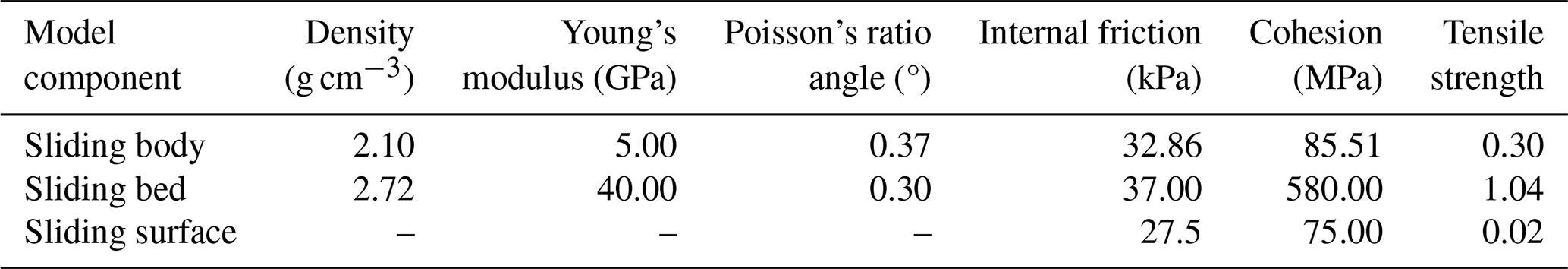
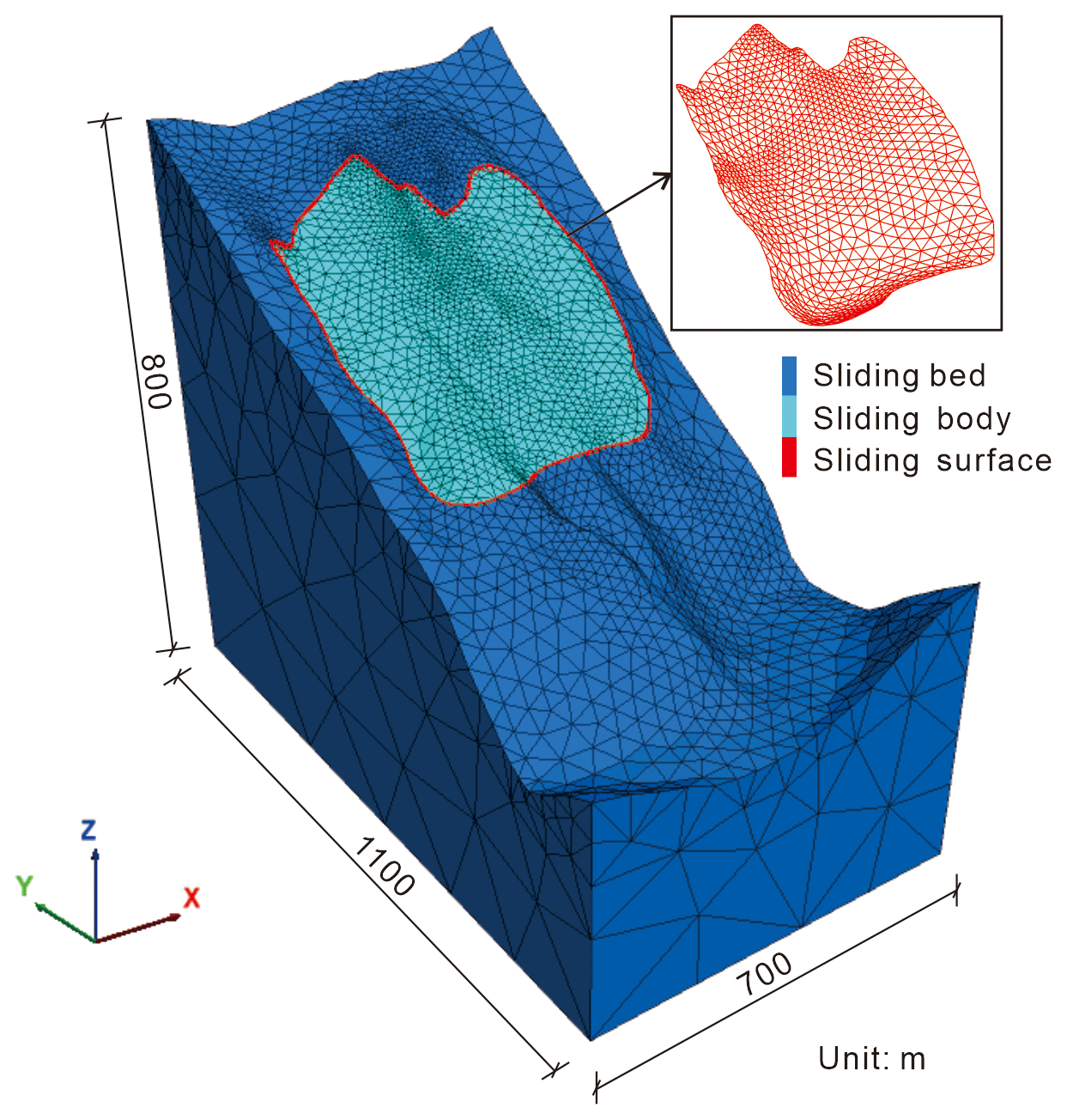
The 3D mesh model of the Tizicao landslide (Fig. 10) was established using the FLAC3D program. It was composed of a sliding bed, a sliding body, and a sliding surface, with a length of 1100 m, a width of 700 m, and a height of 800 m. In this model, the sliding bed and sliding body were established using tetrahedral elements. The sliding surface was established using contact surface elements which allow the contact surface to slide. The geometric size and shape of the 3D sliding surface were deduced according to the depth of the sliding-zone soil obtained by drilling. The parameters such as the area and the position of the locking segment were obtained by Zhou et al. (2022). The constitutive model of Mohr–Coulomb was used in the simulation. The bottom was fixed as a boundary, while the top surface was set as a free boundary. The other four surfaces were set as boundaries with fixed perpendicular displacement. Given that the simulations in this study are only aimed at exploring the deformation and the overall stability of the landslide, the sliding body and sliding bed were supposed to be heterogeneous, while factors such as joints and heterogeneity of rock masses were temporarily not considered. The simulation parameters of the sliding body, sliding bed, and sliding surface in the model were obtained through indoor geotechnical tests (Table 1). Among them, the rock density was obtained using the wax-sealing method; Young's modulus, Poisson's ratio, internal friction angle, and cohesion of rocks were collected from the triaxial test; and the tensile strength was obtained from the Brazilian test.

Table 1 Simulation parameters of the landslide model.

Figure 10 The mesh model and geometry of the Tizicao landslide.

The simulation analysis of the Tizicao landslide was conducted using the three rock bridge models mentioned above. As revealed by site drilling, the rock masses in the locking segment have the same intact degree as the phyllites in the sliding bed. Therefore, the strength parameters of the rock bridges were set at the same values as those of the rock masses in the sliding bed (locking masses) in the IRMM model. Meanwhile, the shear stiffness and normal stiffness of the sliding surface in this model were both set at 2.0 MPa m⁻¹ to simulate the sliding state of the landslide. For the JM model, the rock bridge and sliding surface were both simulated using the contact surface model. According to the site survey, the area of the locking segment accounts for 15.2 % of the total area of the landslide. The equivalent internal friction angle and equivalent cohesion were determined to be 35.68° and 503.24 kPa, respectively, by solving Eqs. (1) and (2). The tensile strength, shear stiffness, and normal stiffness of the sliding surface were set at 0.18 MPa, 1800 MPa m⁻¹, and 1800 MPa m⁻¹, respectively, in the JM model. For the CSM-HSP model, the locking masses were replaced with the contact surface model, whose strength and stiffness were both higher than those of the sliding surface. Their strength parameters were set at the same values as those of the sliding bed. Meanwhile, the shear stiffness and normal stiffness of the contact surface of the rock bridge were both set at 2000 MPa m⁻¹. The strength parameters and stiffness coefficients of the sliding surface in the CSM-HSP were set at the same values as those of the sliding surface in the IRMM since the sliding surface models were the same in FLAC3D.

3.3 The 2D stability simulation

To compare the differences between the 2D and 3D stability of the Tizicao landslide, this study conducted the 2D stability analysis of four sections of the landslide (Fig. 4) using the SLOPE/W module of the program GeoStudio 2012. The SLOPE/W module was used to calculate the 2D stability of slope and landslide (Chen et al., 2020; Jafri et al., 2020). Meanwhile, the JM model was introduced into Bishop's algorithm of the GeoStudio program. Bishop's algorithm is a limit equilibrium method for stability calculations. According to the JM model, the equivalent shear strength parameters were determined based on penetration rates using Eqs. (1) and (2). Then, these parameters were assigned to the sliding surface to calculate the 2D Fos using Bishop's algorithm. The simulation parameters of the sliding body, sliding surface, and locking masses are shown in Table 1. According to the site survey, sections A-A', B-B', C-C', and D-D' have k_L values of 0, 0, 0.23, and 0.26, respectively, and the 2D stability factors calculated are shown in Table 2 and Fig. 11.

Table 2 The 2D and 3D Fos values.

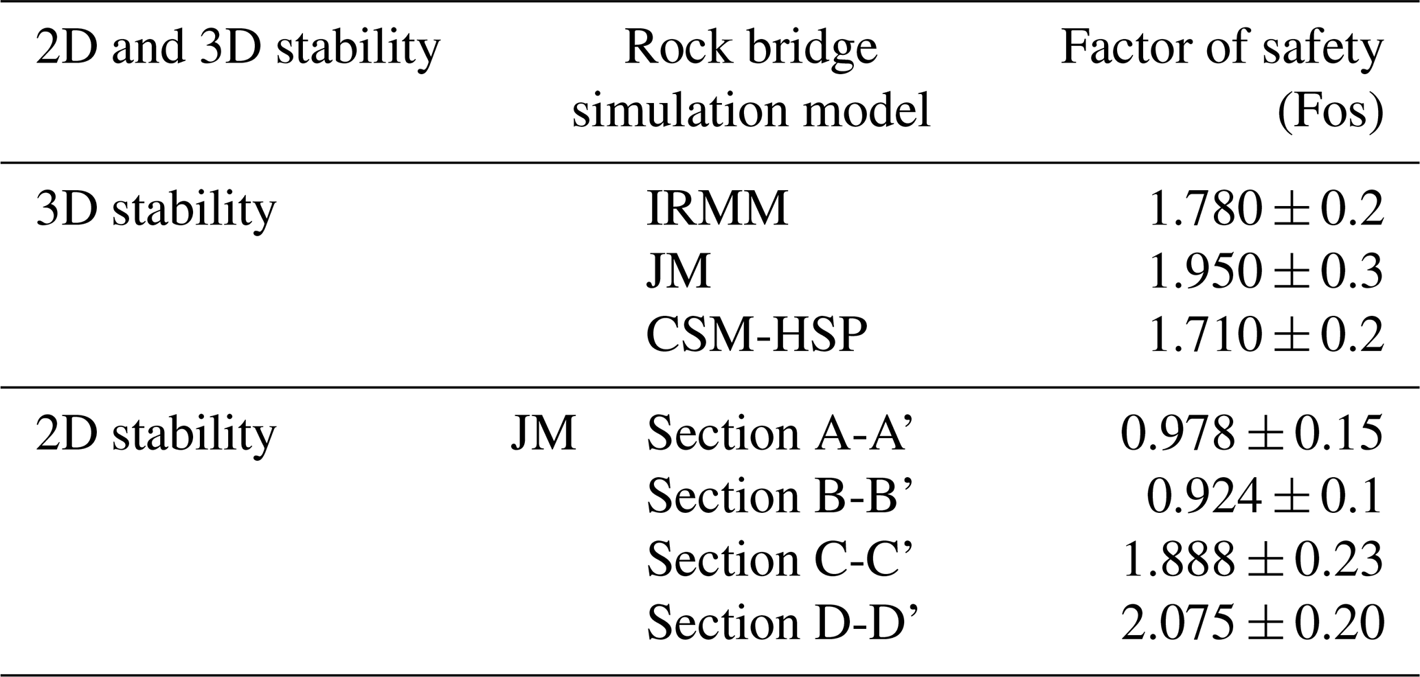
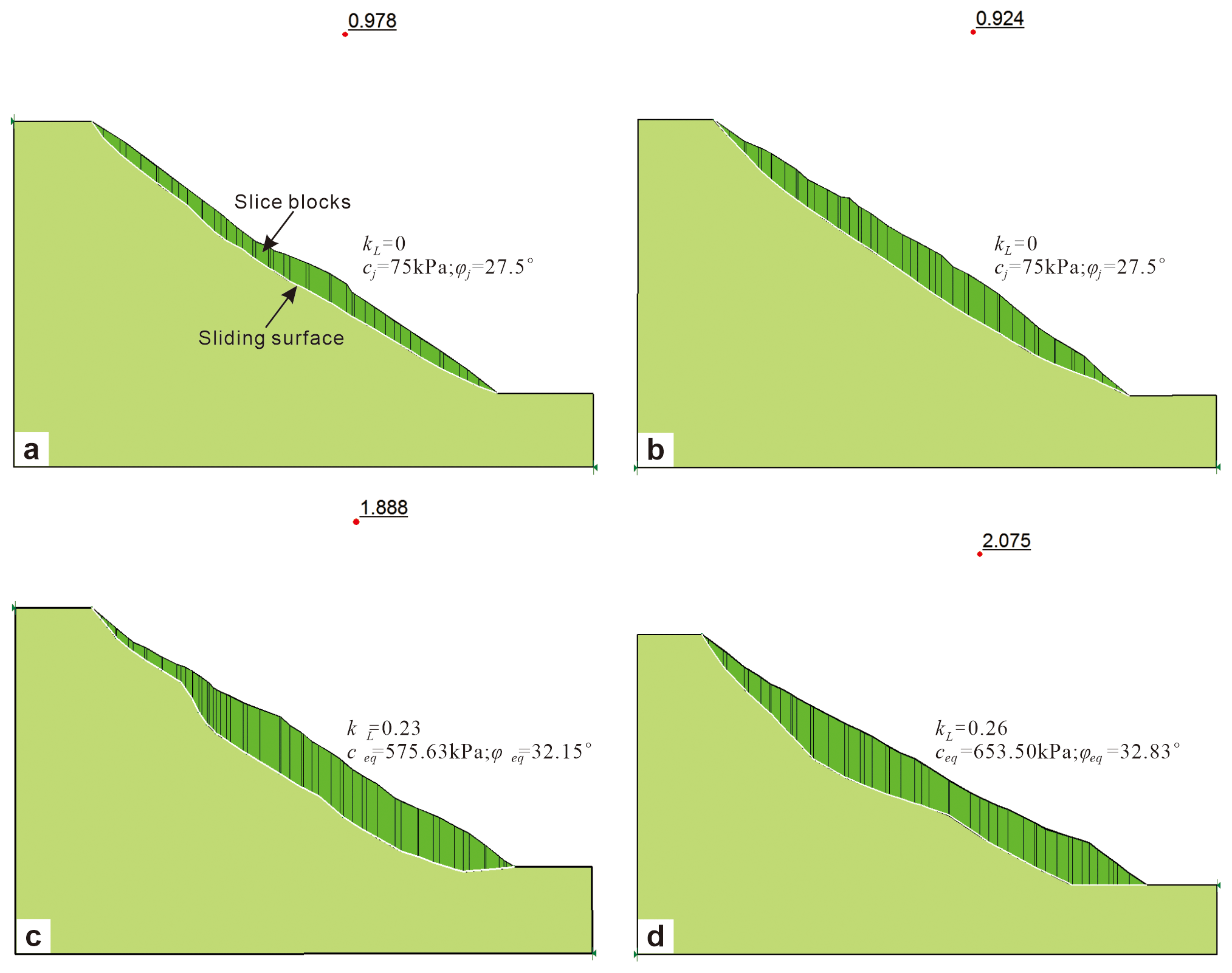
Figure 11 The 2D Fos of different sections. (a) Section A-A'. (b) Section B-B'. (c) Section C-C'. (d) Section D-D'.

4 Results

4.1 Comparative analysis of 2D and 3D stability

Table 2 shows the 3D Fos of the Tizicao landslide obtained using the three models and the 2D Fos of the landslide calculated by using the JM model. The 3D Fos values obtained using the IRMM, JM, and CSM-HSP models were 1.780 ± 0.2, 1.950 ± 0.3, and 1.710 ± 0.2, respectively, which are almost equal, and the average is 1.813. These results indicate that the Tizicao landslide is stable and large-scale sliding will not occur under current conditions. The state of the landslide is consistent with the displacement monitored in the field (Fig. 3c). As shown in Fig. 11, sections A-A', B-B', C-C', and D-D' of the Tizicao landslide had 2D Fos values of 0.978 ± 0.15, 0.924 ± 0.1, 1.888 ± 0.23, and 2.075 ± 0.20, respectively. Therefore, the landslide is unstable along sections A-A' and B-B', which is consistent with the large-scale collapse in the northern front of the landslide (Fig. 2d). In contrast, the landslide is stable along sections C-C' and D-D', and this finding agrees well with the middle and south deformation areas of the landslide. The difference in the landslide stability between the north (sections A-A' and B-B') and south (sections C-C' and D-D') sides of the landslide is primarily caused by the existence of the locking masses in the southern front of the landslide (Fig. 2b). According to Table 2, the 3D Fos of the Tizicao landslide differs greatly from its 2D Fos. For the landslide sections with severe deformation (sections A-A' and B-B'), their 2D Fos values were lower than their 3D Fos values. However, for the landslide sections with slight deformation (sections C-C' and D-D'), their 2D Fos values were significantly greater than their 3D Fos values, especially for the landslide sections with the locking segment. The relatively conservative 2D stability analysis (Li et al., 2010; Park and Michalowski, 2017) made the 2D Fos values usually lower than the 3D Fos values. Nonetheless, for the landslide sections with rock bridges, their 2D Fos values may exceed their 3D Fos values (Table 2). The overall stability of a landslide with rock bridges should be assessed using 3D Fos since the 2D Fos represents only the local stability of the landslide.

4.2 Analysis of landslide deformations

According to the above analysis, all the IRMM, JM, and CSM-HSP models can be used to effectively simulate the overall stability of 3D landslides and obtain their 3D Fos. However, the JM model cannot simulate real 3D deformation behaviors of landslides since it uses equivalent strength parameters. Meanwhile, the IRMM model is subjected to rather complex modeling although it can be used to obtain real 3D deformation characteristics of landslides. Therefore, the CSM-HSP model was selected to simulate the deformation trend of the Tizicao landslide. Figure 12a–d show the total displacement contours of the sliding body, the shear displacement contours and the sliding state of the sliding surface, and the sliding velocity vectors of the sliding surface, respectively.

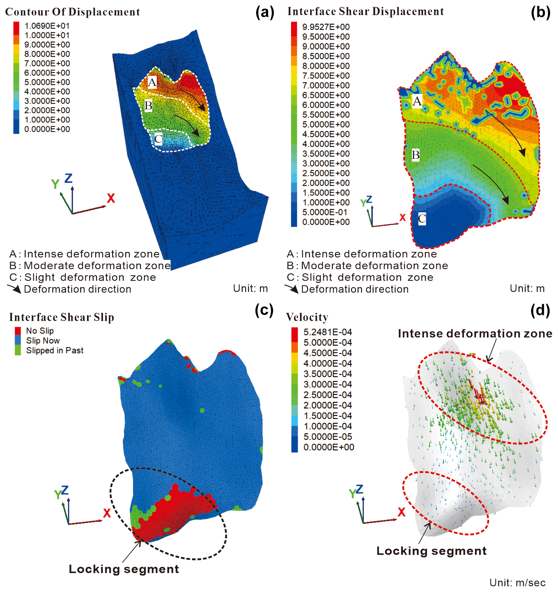
Figure 12 Simulation results of the Tizicao landslide. (a) Total displacement contours. (b) Shear displacement contours of the sliding surface. (c) Sliding state of the sliding surface. (d) Sliding velocity vectors of the sliding surface.

As shown in the isoline map of surface displacement (Fig. 3b), a sliding event occurred in a general northeast direction (closer to the north) from 13 August 2017 to 25 January 2018. In this event, the maximum surface displacement (1210 mm) occurred at the northern toe, which coincided with the location where the front collapsed (Fig. 2d). The landslide's rear and middle parts showed similar surface displacement of 150–300 mm in the sliding event, indicating that they slid as a whole. The minimum surface displacement of 30–150 mm occurred in the southern area of the slope toe throughout the whole sliding event. Therefore, the southern area serves as the anti-sliding area of the whole landslide.

As shown in Fig. 12a, the total displacement contours of the sliding body show significantly different deformation zones, namely the intense deformation zone from the rear to the north side wall of the landslide, the moderate deformation zone from the middle part of the landslide to the northern part of the landslide front, and the slight deformation zone in the middle and southern parts of the landslide front. The maximum displacement of the sliding body is 10.69 m at the landslide's rear (Fig. 12a), which agrees with the width of crack L07 (Fig. 13). Figure 12a shows that the Tizicao landslide tends to slide northeastward generally owing to the sliding resistance of the locking segment. This tendency is consistent with the crack distribution (Fig. 3a) and the isoline map of surface displacement (Fig. 3b). Figures 12a and 3a show different displacement values because the monitoring data obtained from 13 August 2017 to 25 January 2018 (after the large deformation in July 2017) were not the complete deformation data of the landslide. In contrast, Figs. 12a and 3a reflect the same deformation tendency.

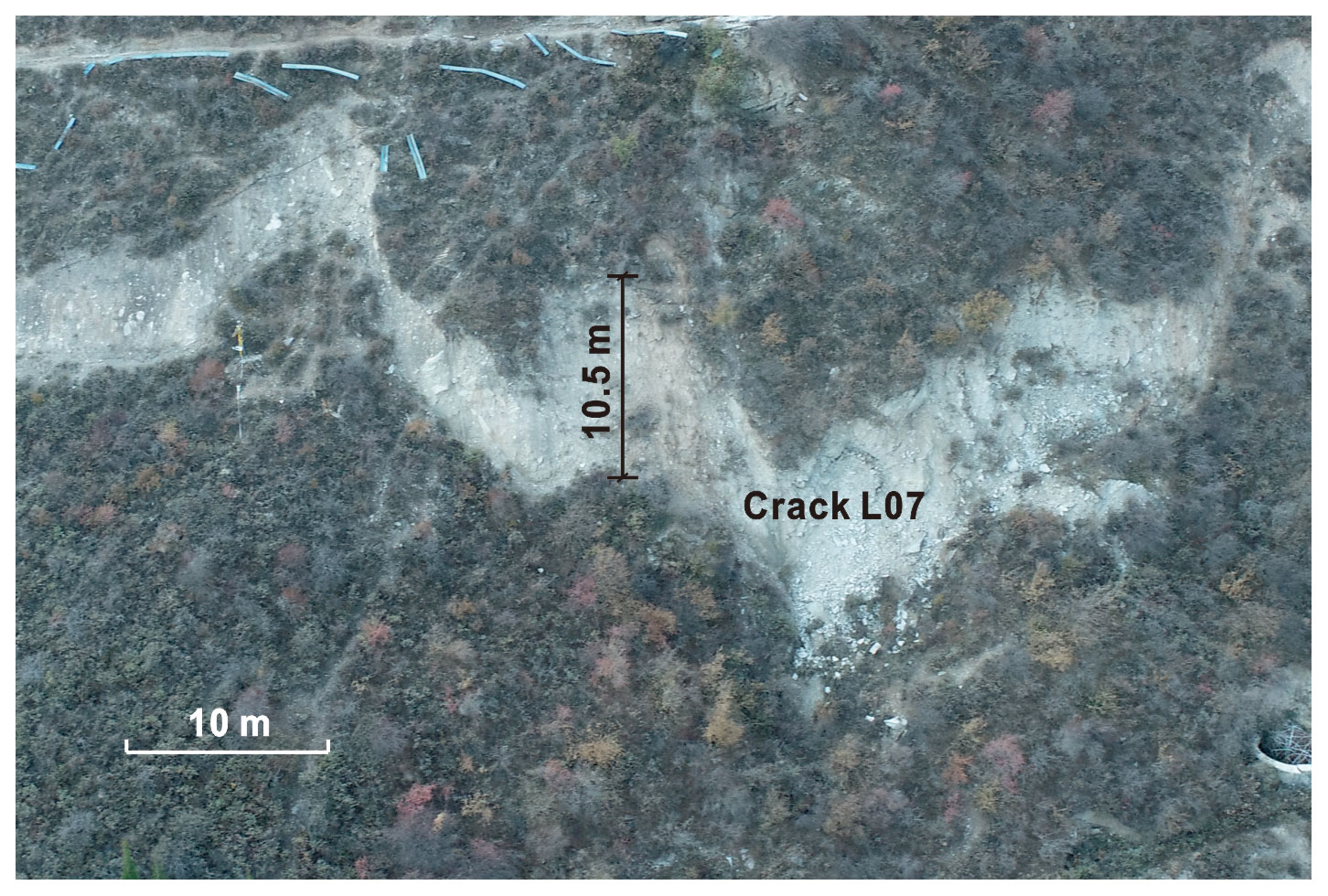
Figure 13 Crack L07 at the rear of the landslide. The width of crack L07 is 10.5 m in the direction of the landslide.

Figure 12b shows that the shear deformation of the sliding surface agrees well with the total displacement contours (Fig. 12a). According to this figure, the shear displacement of the sliding surface is 0 at the position of the locking segment. Figure 12c shows the sliding state when the Tizicao landslide is in equilibrium under current conditions. The red, blue, and green zones in Fig. 12c represent the sliding surface areas where sliding has not occurred, is occurring, and has occurred, respectively. Therefore, no shear displacement occurs in the locking segment on the sliding surface, and the 3D locking segment along the sliding surface can be observed. The sliding velocity vector diagram of the sliding surface (Fig. 12d) indicates that the sliding velocity is low and tends to be 0 in the locking segment. Therefore, the existence of the locking segment is the fundamental reason for the absence of large-scale sliding in the whole landslide.

5 Discussion

5.1 Effects of the locking ratio on 3D stability

To establish landslide models with different locking ratios, rectangular wireframes were used to cover the outline of the landslide (Fig. 14), and the lengths and widths of the wireframes and their ratios were obtained. Rectangles with increasing lengths and widths but a fixed length / width ratio were used to gradually match the landslide from the southern part of the front to the rear in the north. Then, the coverage areas and positions of the 3D sliding surface were obtained as the actual locking ratio changed from 0 to 1 (interval: 0.1). Accordingly, the 3D modeling of the Tizicao landslide was conducted using the three rock bridge models.

Figure 14 Locking areas under different locking ratios.

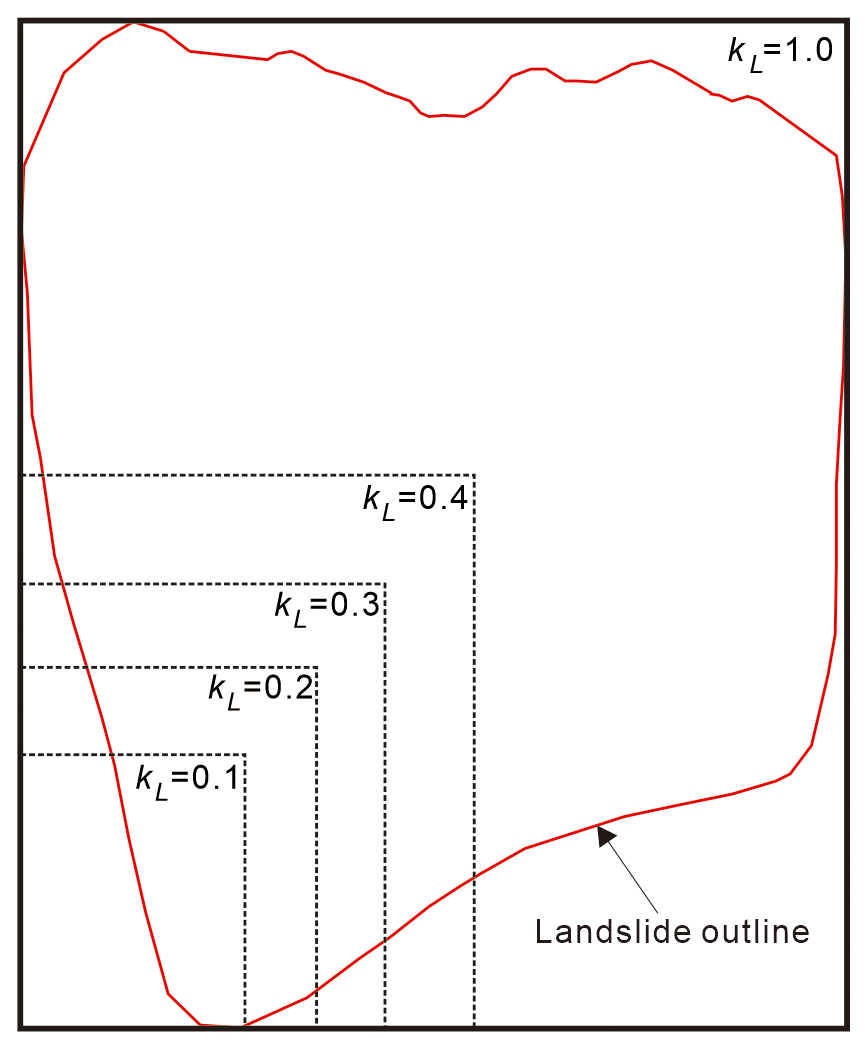
Figure 15 shows the 3D Fos curves of the landslide under different locking ratios. According to this figure, the 3D Fos curves obtained using the three rock bridge models were roughly the same. In detail, they were parabolas overall, and all the Fos values first increased and then tended to be stable as the locking ratio increased. According to the field survey, the Tizicao landslide has an actual locking ratio of 0.152, corresponding to the 3D Fos values of 1.71–1.95. When the locking area of the landslide decreased gradually to 0 (no locking segment), the 3D Fos of the landslide would be 1.215, decreasing by 29.0 %–37.7 % compared to the 3D Fos under current conditions. In this case, the landslide would be unstable. This indicates that the locking segment has significant effects on the overall stability of the landslide.

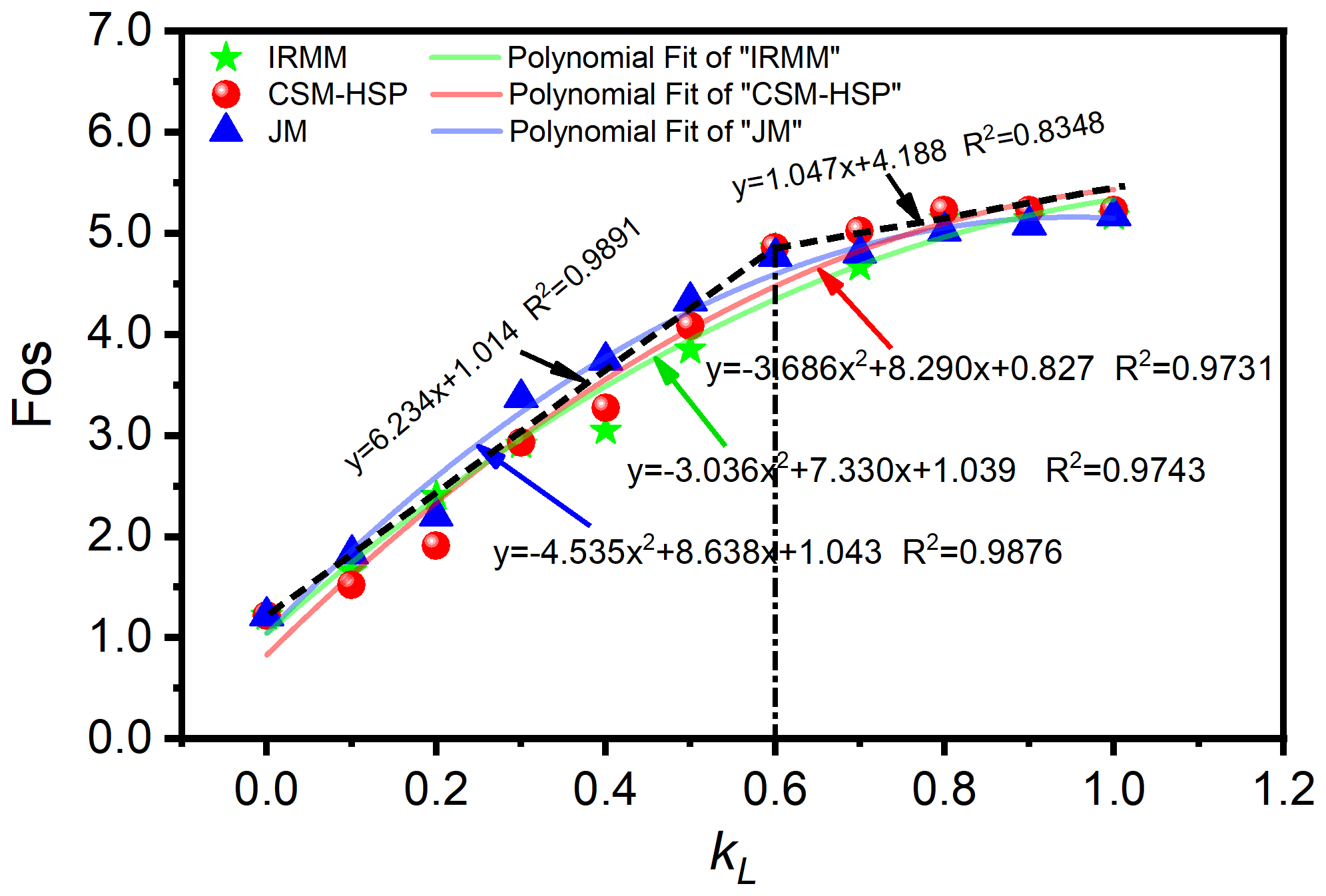
Figure 15 The 3D Fos curves under different locking ratios obtained using three rock bridge models.

According to Eq. (4), there exists a linear relationship between the locking ratio and the Fos, which applies to the 2D stability of landslides subjected to planar sliding (Jennings, 1970). However, the Fos of 3D landslides with a locking segment varied with the locking ratio in the form of an approximate quadratic parabola under the influence of the positions of locking masses and the curvature of the sliding surface (Fig. 15). As per Bonilla-Sierra et al. (2015), the upper, middle, and lower parts of the coplanar landslide have distinct mechanical failure modes (shear, tensile, or shear–tensile) for a landslide with rock bridges; thus the positions of locking masses would change the 3D stability of the landslide. Additionally, with a decrease in the locking ratio, the critical cohesion decreases nonlinearly (Bonilla-Sierra et al., 2015), and the Fos of the landslide presents a nonlinear rather than a linear trend. This study did not explore the effects of the curvature of the sliding surface on the 3D stability of the landslide with rock bridges. However, it should be further discussed in future research.

As shown in Fig. 15, the 3D Fos curves are significantly piecewise, and two linear fitting curves (dashed black lines) of the 3D Fos were determined. The varying rate of the 3D Fos under a locking ratio of less than 0.6 was significantly higher (about 6 times) than that under a locking ratio of more than 0.6. Therefore, in the case of a high locking ratio (a low penetration rate) of the landslide, the change in the locking ratio has a small impact on the overall stability of the landslide. In contrast, the overall stability of the landslide would decrease significantly as the locking ratio decreased to less than 0.6. Based on the statistics of the rock bridge content in rock slope failure obtained by Tuckey and Stead (2016), rock slope failures generally exhibit a rock bridge content between 0.2 %–45 %, which was lower than that obtained in this study (60 %). Therefore, rock slope failures usually occur in the case of very low rock bridge content. This is the immediate cause of the result that the Fos of the landslide decreases rapidly and the landslide suffers a dramatic failure under the critical failure condition.

5.2 Effects of the strength parameters of the sliding surface and locking masses on 3D stability

To estimate the effects of the strength parameters of the sliding surface and locking masses on the 3D stability of the landslide, the strength parameters were obtained through the direct shear test of soils or cores drilled. The cohesion and internal friction angle of the locking masses were determined to be 10–20 000 kPa and 20–65°, respectively, while those of the sliding surface were calculated at 6–1000 kPa and 5–35°, respectively. Then, the 3D Fos curves under different strength parameters and a locking ratio of 0.5 were derived from the three rock bridge models, as shown in Fig. 16. According to Fig. 16a, the 3D Fos increased rapidly when the cohesion of the locking masses was 10–1000 kPa and then became stable when the cohesion exceeded 1000 kPa. Therefore, the 3D Fos was sensitive to the cohesion of the locking masses in the range of 10–1000 kPa but did not significantly vary when the cohesion was greater than 1000 kPa. The cohesion of the sliding surface on the 3D Fos exhibited different effects (Fig. 16c). With an increase in the cohesion of the sliding surface, the 3D Fos obtained using IRMM and CSM-HSP first increased nonlinearly and then stabilized, while the 3D Fos obtained using the JM increased at a decreased acceleration rate.

Figure 16 The 3D Fos curves under different strength parameters.

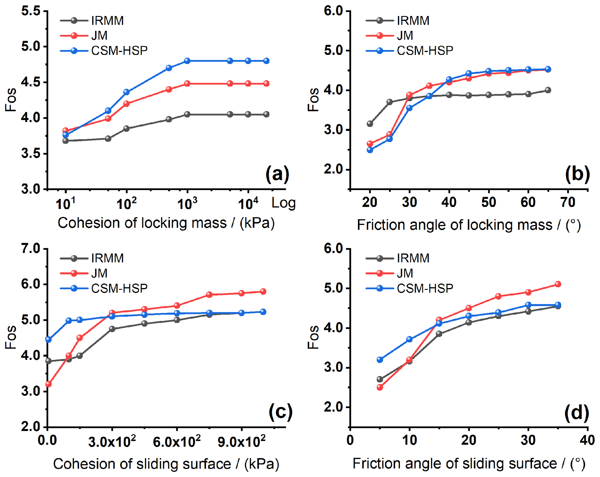
As shown in Fig. 16b, the 3D Fos of the landslide first increased nonlinearly and then stabilized with an increase in the internal friction angle of the locking masses. It increased from 2.49 to 4.53 (1.82 times) as the friction angle of the locking mass increased from 20 to 65°, with an average growth rate of 0.045. The 3D Fos of the landslide varied with the internal friction angle of the sliding surface in a similar trend (Fig. 16d). Specifically, the 3D Fos increased from 3.20 to 4.58 (4.13 times) as the internal friction angle of the sliding surface increased from 5 to 35°, showing an average growth rate of 0.046. The comparison of the average growth rates reveals that the internal friction angles of both the locking masses and the sliding surface have almost the same effects on the 3D Fos of the landslide.

5.3 Comparative analysis of the three rock bridge models in the numerical simulation program

The IRMM, JM, and CSM-HSP models yielded almost equal 3D Fos values (Fig. 15), indicating that the three models can be used to effectively simulate the overall stability of a landslide with a locking segment. The IRMM model (Fig. 9a) is frequently used to simulate the stability and the deformation and failure behaviors of 2D and 3D rock slopes with rock bridges (Zhang et al., 2014; Hu et al., 2018). This model can simulate the actual deformation process of the slopes and is one of the most effective models in the simulation of rock slopes and landslides. However, the IRMM model requires accurate information such as the area and position of a locking segment. Accordingly, it is necessary to identify a locking segment of a landslide in detail before stability analysis, which is quite difficult due to the concealment of locking masses (Elmo et al., 2018; Guerin et al., 2019). Meanwhile, the uncertain position and irregular geometric size of a locking segment also pose great difficulties for landslide modeling. The JM model (Fig. 9b) cannot be used to further analyze the deformation and failure behaviors of landslides and obtain actual deformation since it ignores the positions of rock bridges and the response of rock bridges to the landslide deformation (Einstein et al., 1983). However, the 3D Fos of landslides (Figs. 15–16) can be obtained using this model. Therefore, the JM model can be used to only analyze the macroscopic 3D stability of landslides. Moreover, the JM model is unsuitable for the 3D stability analysis of rock landslides with a sliding surface dipping over 50° due to their high probability of tensile failures. For the CSM-HSP model (Fig. 9c), two contact surface models, one with high strength parameters and the other with low strength parameters, can be used to simulate the rock bridge and the sliding surface, respectively. This model integrates the advantages of the IRMM model in terms of simulating the actual deformation of slopes with rock bridges and the advantages of the JM model in terms of modeling. Using this model, the overall deformation and Fos of landslides can be obtained, and the position and area of a locking segment can be changed at will, thus greatly reducing the workload in the modeling of landslides with rock bridges. The CSM-HSP model outperforms the other two models in simulating both the 3D stability and the deformation and failure behaviors of landslides with a locking segment.

6 Conclusions

All the IRMM, JM, and CSM-HSP models can be used to obtain the 3D Fos of landslides with a locking segment each, providing convenient and effective simulation approaches for assessing and predicting the 3D stability of the landslides. The simulation results indicate that the Tizicao landslide is generally stable under current conditions owing to the existence of the locking segment in the southern front. This conclusion is consistent with the deformation and failure characteristics, the position and area of the locking segment, and the site monitoring data of the Tizicao landslide. As indicated by the comparison between the results of 3D and 2D stability analyses of the Tizicao landslide, the 2D stability analysis is suitable only for local stability, while the 3D stability represents the overall stability of landslides with a locking segment each. As shown by the discussion, there is a linear relationship between the locking ratio and 2D Fos of landslides with a locking segment each that are subjected to planar sliding, while there exists an approximate quadratic parabola between the locking ratio and 3D Fos of landslides with a locking segment each under the influence of the positions of the locking masses and the curvature of the sliding surface. The increase in the strength parameters of both the locking segment and the sliding surface can improve the stability of landslides nonlinearly. The 3D Fos of the landslides is sensitive to the cohesion of both the locking segment and the sliding surface in the range of 10–1000 kPa. The internal friction angles of the locking masses and the sliding surface have almost the same effects on the 3D Fos of landslides. The CSM-HSP model integrates the advantages of the IRMM model in terms of simulating the actual deformation of slopes with rock bridges and the advantages of the JM model in terms of modeling. Therefore, this model outperforms the other two models in simulating both the 3D stability and the deformation and failure behaviors of landslides with a locking segment each.