Mapping current and future flood exposure using a 5 m flood model and climate change projections

Local stakeholders need information about areas exposed to potential flooding to manage increasing disaster risk. Moderate- and large-scale flood hazard mapping is often produced at a low spatial resolution, typically using only one source of flooding (e.g., riverine), and it often fails to include climate change. This article assesses flood hazard exposure in the city of Vancouver, Canada, using flood mapping produced by flood risk science experts JBA Risk Management, which represented baseline exposure at 5 m spatial resolution and incorporated climate-change-adjusted values based on different greenhouse gas emission scenarios. The article identifies areas of both current and future flood exposure in the built environment, differentiating between sources of flooding (fluvial, pluvial, storm surge) and climate change scenarios. The case study demonstrates the utility of a flood model with a moderate resolution for informing planning, policy development, and public education. Without recent engineered or regulatory mapping available in all areas across Canada, this model provides a mechanism for identifying possible present and future flood risk at a higher resolution than is available at a Canada-wide coverage.

1 Introduction

The exposure of people and infrastructure to flood hazards is increasing globally due to factors such as population growth, development in flood-prone areas, and more frequent and intense extreme weather caused by climate change (Field et al., 2012; UNDRR, 2022). Moreover, it is expected that all major types of flooding, including fluvial (riverine), pluvial (rainfall), and storm surge (coastal), will intensify as the climate changes (Alfieri et al., 2016; Arnell and Gosling, 2016; Hirabayashi et al., 2021; IPCC, 2019; Muis et al., 2016; Winsemius et al., 2016).

Coastal cities are especially susceptible to flooding due to their dense populations, socioeconomic development, impervious surfaces, and proximity to major hydrological features such as lakes and oceans (Hallegatte et al., 2013; Lincke et al., 2022; McDermott, 2022; Neumann et al., 2015). Managing flood risk in coastal cities requires adopting actions that allow us to reduce the vulnerability of people and property to current flood hazards and anticipate the likely scope and extent of future flooding. Flood hazard modelling and mapping that use climate scenarios to estimate future flood exposure enable coastal cities to better support flood risk management, inform land use planning, organize emergency management, and increase public awareness (Dransch et al., 2010; Handmer, 2013; Porter and Demeritt, 2012).

Despite the importance of flood hazard mapping for flood risk management, few studies have mapped community exposure to multiple flood types and used future climate scenarios to assess changes to exposure (Cea and Costabile, 2022). Modelling techniques to estimate flooding under different climate scenarios vary considerably in existing scholarship, and the quality and granularity of local and regional flood maps are also highly variable (Cea and Costabile, 2022; Costabile et al., 2015; de Moel et al., 2009; Henstra et al., 2019; Mudashiru et al., 2021). These limitations underscore the need to develop flood hazard models and maps that capture flood exposure accurately and at a resolution that is useful for planning and decision-making.

The purpose of this paper is to expand on traditional physically based flood exposure modelling and mapping methodologies that often lack consideration of multiple flood mechanisms and climate change at a high resolution. This paper presents the results of a flood model that was used to produce flood hazard maps under various climate change scenarios for the city of Vancouver, Canada. Using a 5 m resolution baseline and climate change-adjusted flood data produced by flood risk science experts at JBA Risk Management (JBA), we determined areas of existing building exposure to multiple flood types, as well as new exposure based on climate change scenarios for 2050 and 2080. The findings demonstrate the utility of local and regional flood exposure analysis using different climate change scenarios, which offers guidance for local planners, policy- and decision-makers, and other stakeholders to recognize areas of current and future flood risk and enact measures to manage this risk.

The paper begins by reviewing current scholarship on flood hazard mapping to distinguish different methodologies, assess their applicability in Canada and beyond, and identify knowledge gaps. It then describes the flood hazard mapping approach used in this study and its application in Vancouver. The fourth section reports the study's main findings. The paper concludes with a broader discussion on the strengths and limitations of the method, directions for its use in local and regional planning, and areas for future research.

2 Literature review: flood hazard mapping methodologies

Scholarship on flood hazard mapping has been increasing for decades. Early approaches to flood hazard modelling were incapable of incorporating long-term climate projections and variations to hydrological processes (Batista, 2018). More contemporary approaches rely on computer modelling and mapping that can apply scenario-based projections of climate change and precipitation (Mudashiru et al., 2021; Teng et al., 2017). This section reviews current scholarship on methodologies for modelling flood exposure and its application in Canada with climate change.

2.1 Modelling flood exposure

There are three main methodologies for producing flood hazard maps: physical modelling, physically based modelling, and empirical modelling (Mudashiru et al., 2021; Teng et al., 2017). Physical models map flood hazards using field measurements and observations of hydrological features, such as the velocity and flow of a meandering river (Mubialiwo et al., 2022; Paquier et al., 2017). Physical models produce the most accurate and highest-resolution pictures of flood hazards (e.g., 1 m), but the on-site measurement and testing requirements are onerous, time-consuming, and costly, such that these models are typically limited to a small spatial coverage (Bellos, 2012).

Physically based models simulate real-world hydrological processes to identify areas that could be inundated under various conditions (e.g., extreme weather, riverine flow patterns) (Mudashiru et al., 2021). These models are increasingly relied on by flood risk management practitioners because of their capacity to integrate 1- (1D), 2- (2D), and 3-dimensional (3D) hydrodynamic models (Anees et al., 2016). One-dimensional models are mostly adopted for river studies when the computational requirements required to estimate flood exposure are more limited (Horritt and Bates, 2002; Dazzi et al., 2021). Meanwhile, 2D approaches are becoming more common in the field of flood hazard modelling and mapping due to increased access to digital terrain models for geographically large areas (Dazzi et al., 2021). However, the computational requirements to run sophisticated flood models using 2D hydrodynamic models over a large area are significant. In data-sparse regions and areas where data acquisition and procurement are more limited due to administrative constraints, access to high-quality 2D approaches may be hindered. Similarly, while 3D models provide a more nuanced examination of flood hazard exposure, the computational requirements to run such a model are prohibitive, as mapping the results requires specialized technical expertise. Overall, physically based models reduce the need for field observations, which are instead simulated in a lab, enabling researchers to extrapolate field observations to cover a larger area in less time. However, the accuracy of these maps is sometimes challenged by critics who question assumptions about the hydrological processes that have not been fully tested in the field (Costabile et al., 2015; Mark et al., 2004).

Empirical modelling is a more recent development in flood hazard assessment that typically combines satellite imagery, remote sensing, machine learning, artificial intelligence, and geographic information systems to predict areas exposed to flood inundation (Devia et al., 2015). This approach has become more common in conventional flood hazard mapping because it can produce maps with large spatial coverage, it is less onerous and more efficient than physical and physically based models from a cost–benefit perspective, and it is capable of incorporating environmental changes such as those associated with climate change (Jehanzaib et al., 2022; Mosavi et al., 2018; Mudashiru et al., 2021). However, empirical models typically produce lower-resolution maps (e.g., 30 m or lower) and make broader assumptions about physical conditions than physical and physically based models (Avand et al., 2022; Li et al., 2013; Woznicki et al., 2019).

Physically based maps producing high levels of accuracy tend to be costly and require significant resources and time, whereas empirical models are less accurate but require less resources and can be deployed at a broader scale. Policymakers must assess these trade-offs when determining which maps should be generated for specific locations and audiences. For example, small and remote communities might lack the financial capacity to conduct physical modelling, so a cost-efficient, multiple-return-period model might be desirable, as it can map hazard exposure and incorporate climate change projections at a moderate resolution that is sufficient for planning and decision-making. For this reason, this study used a physically based modelling approach as a sensible middle ground and starting point. The next section describes the evolution of flood mapping in Canada and how maps are used in flood risk management.

2.2 Modelling Canada's flood exposure under climate change scenarios

Despite the value of flood hazard maps for land use planners, emergency managers, and other stakeholders, several factors limit their utility in practice. In particular, many existing flood hazard maps lack high-resolution data, fail to represent multiple sources of flooding (e.g., fluvial, pluvial, and storm surges), and neglect to incorporate the influence of climate change on flood exposure (Cea and Costabile, 2022; de Moel et al., 2009; Teng et al., 2017). Moreover, the variable accuracy and reliability of flood hazard maps produced through different modelling approaches, often with different assumptions and using coarse resolution data, as well as the technical and financial requirements to produce higher-quality maps, often hinder their availability and effective use by non-expert stakeholders, such as planners and policymakers (Dransch et al., 2010; Hagemeier-Klose and Wagner, 2009; Pralle, 2019; Wing et al., 2018).

Flood hazard mapping in Canada is highly variable due in part to the country's large geographic area and diverse topography (Elshorbagy et al., 2018). Flood mapping is a provincial and territorial responsibility, with some provinces and territories performing mapping in-house, while others contract flood mapping to private industry (Natural Resources Canada, 2022). Because provincial governments have the primary responsibility to map flood hazard, there is a patchwork of coverage and map availability across Canada. Further, despite recent data initiatives to compile flood data (Natural Resources Canada, 2023), there is no national, high-resolution physical modelling for all of Canada.

There are significant gaps in flood mapping coverage across Canada, and the dominant focus of nearly all regulatory flood mapping is fluvial (riverine) flooding. To date, physically based flood hazard modelling has been relatively unavailable in Canada, particularly modelling that includes widespread coverage, captures multiple sources of flooding, and accounts for climate change (MMM Group Limited, 2014). However, few commercial risk modelling companies offer solutions with national or near-national coverage that include areas not otherwise mapped in Canada. Whereas organizations such as the First Street Foundation and Fathom offer comprehensive coverage of the United States and elsewhere, no such modelling in Canada has been completed. To accomplish such large-scale modelling, considerable climate modelling, hydraulic modelling, data collection, and computational resources are required. Such models can be a useful source of flood intelligence as computational and physically based modelling improves in accuracy with advancements in data availability and computational resources.

Against this backdrop, we present here an assessment of flood exposure using JBA's physically based flood hazard model at a 5 m resolution that includes multiple flood types – fluvial, pluvial, and storm surge – and estimates future changes due to climate change based on the Representative Concentration Pathway (RCP) 4.5 and 8.5 climate scenarios. We apply this model using a case study of the city of Vancouver, British Columbia, which faces risks from all three flood types. This study illustrates a practical application of physically based modelling for the purposes of generic flood exposure assessment and flood risk planning.

3 Methods

This section describes the methods used to harness the physically based flood hazard model and its application to the city of Vancouver. It includes an overview of the study area and research methods that were used to assess the current and projected changes to local flood exposure based on climate change scenarios, multiple sources of flooding, and time horizons.

3.1 Study area

The scope of this assessment was limited to the JBA Canada 5 m Baseline and the Climate Change Flood Data study site for the Vancouver area (JBA Risk Management Limited, 2022). This dataset contained fluvial, pluvial, and storm surge flood hazard data under non-climate-change (NCC) and climate change states, specifically RCP4.5 and RCP8.5 climate scenarios for 2050 and 2080. The flood hazard data were produced by JBA and shared with the University of Waterloo research team for the Vancouver metropolitan area. This area delineates 117 contiguous census tracts in the city from the 2016 open census tract boundary file (Statistics Canada, 2019). A breakdown of the fluvial, pluvial, and storm surge flood mechanisms in Vancouver is provided in Fig. 1 at the non-climate-change (NCC) state and at the 100-year return period, utilized for illustrative purposes.

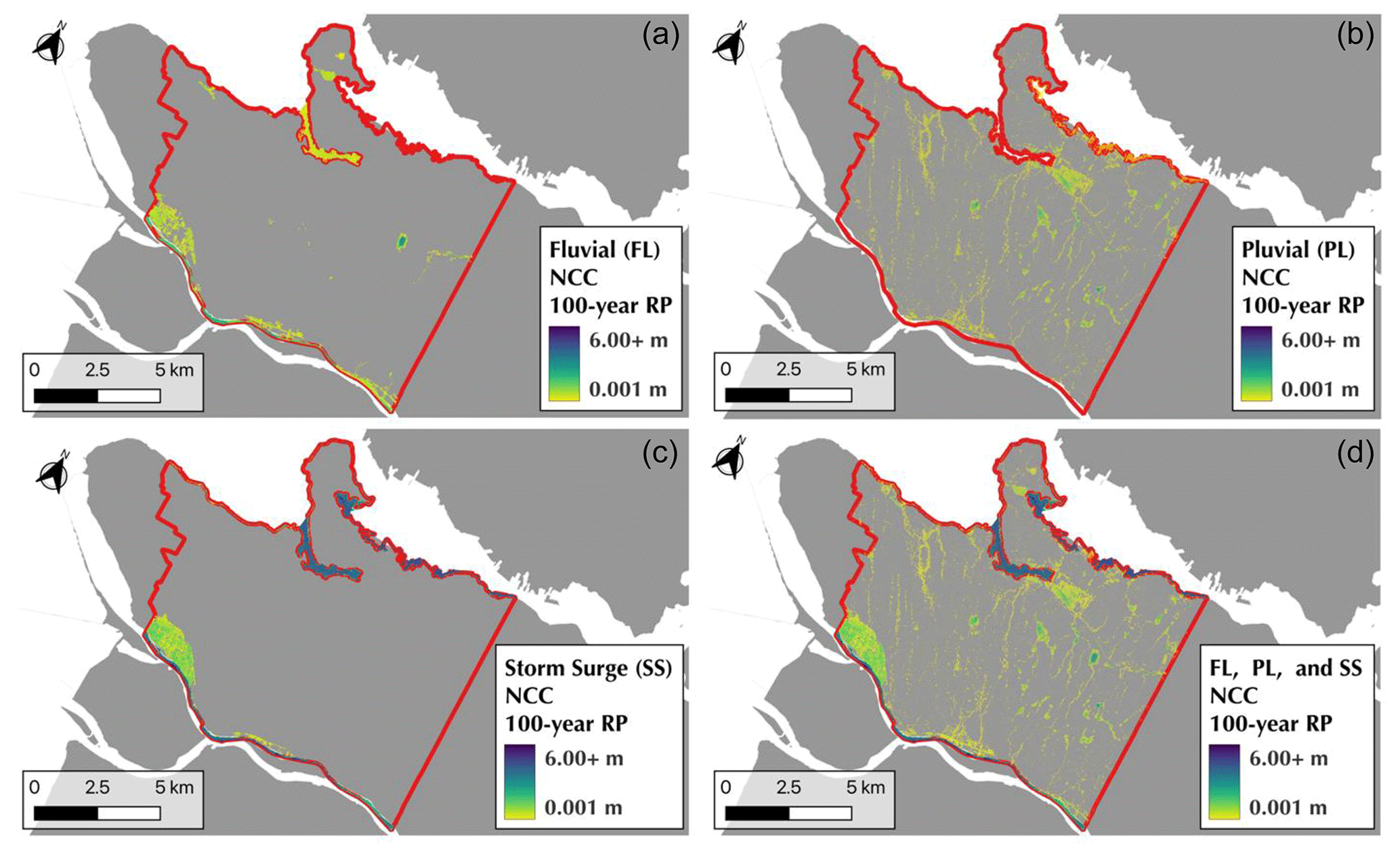
Figure 1 Study boundary of the JBA (2022) flood hazard data for Vancouver, British Columbia, for the fluvial, pluvial, and storm surge flood hazard modelling at the 100-year return period non-climate-change state. All three flood mechanisms are provided in the same map (d) to illustrate the overall flood exposure independent of flood mechanism. Other map data include the Statistics Canada (2022) province and territory boundary file of Canada and the combined census tract boundary forming the study area from Statistics Canada (2019).

The study area illustrated in Fig. 1 is used for the remainder of the assessment. An example exposure dataset provided by Microsoft (2019) was incorporated to indicate the types of analysis that could be conducted using the JBA data.

3.2 Research methods

This study is based on JBA's Canada 5 m Flood Data, baseline and future (and Canada-wide 30 m flood hazard data), obtained through a data-sharing agreement with the University of Waterloo. JBA's in-house two-dimensional hydrodynamic flood model, JFlow (see Lamb et al., 2009, for more information), was used to map fluvial and pluvial flood extents and depths. JFlow solves the shallow-water equations to simulate flooding and is configured differently to generate the pluvial and fluvial flood maps (e.g., modelling along a river network or across pluvial rainfall catchments). The modelling was performed on the best available terrain data, which included 1 m lidar in the Vancouver urban area. The terrain data were used to derive river locations and catchment boundaries and were processed and edited to improve quality (e.g., by removing structures such as bridges which block the natural flow of water). The hydrological inputs required by the hydraulic model vary for different configurations. Depending on catchment size, separate model set-ups were used to represent the different ways small and large rivers respond to storm events.

Rivers draining areas greater than 400 km² were classed as “large rivers” and were modelled to create the fluvial flood maps. For these rivers, the hydrographs for each return period being modelled were derived from a statistical analysis of flood peak gauge data extrapolated from the Water Survey of Canada's HYDAT database (Environment and Climate Change Canada, 2018). To perform this analysis, the median annual maximum flood (QMED) was calculated, representing the 2-year river flow return period. QMED was directly identified for gauged stations with a minimum data record of 10 years. At ungauged locations, QMED was statistically derived, accounting for regional and local climatic factors. After QMED had been calculated for all locations, this was scaled to generate peak flow data for the return periods required using flood growth curves. A flood growth curve describes the ratio between the QMED flow and those at other return periods. The impact of snowmelt was implicitly accounted for in the peak flow data analysis. The design flood depths were turned into hydrographs that represent the volume of water through time and routed through JFlow.

Rivers draining less than 400 km² were classed as “small rivers and pluvial maps”. Small river and pluvial catchments are more responsive to highly localized, intense rainfall than large rivers; therefore, a different approach was applied to capture the maximum likely flood hazard in these smaller catchments. The approach used, referred to as direct–rainfall modelling, estimates design rainfall hyetographs (the distribution of rainfall intensity over time). Rainfall intensity–duration–frequency statistics available from Environment and Climate Change Canada were used to interpolate rainfall estimate data for all catchments. A range of design storm durations were modelled to identify the critical rainfall duration, or maximum likely flood hazard, in each catchment. Short, intense rainfall events tend to generate more flooding in steep-sided valleys, whereas flatter regions are often adversely affected by slower-moving storms with longer storm durations. To account for this, rainfall totals for 1, 3, and 24 h storm durations were used to create multiple modelled flood extents per return period. The flood extent with the greatest water depths was then used for each modelled return period. These estimated rainfall data were used to generate storm hyetographs, and an infiltration coefficient was applied to remove the proportion of rainfall that would infiltrate the ground due to urban drainage, infiltration, and interception. This varies across different land surfaces and climate types defined using the eco-geographical divisions, called ecozones, from the National Ecological Framework of Canada (Agriculture and Agri-food Canada, 2023). For urban areas, a runoff value of 85 % was applied (i.e., 15 % loss). This value was selected based on the well-established US Soil Conservation Service (SCS) curve number method (USDA, 1986) where high numbers represent higher runoff (e.g., 98 for completely paved and 46 for low-density residential areas with permeable soil). After sensitivity testing of curve numbers, an infiltration coefficient of 85 was selected as a single best value to represent Canadian urban areas. The impacts of seasonality, including the role of frozen ground and seasonal snowmelt, were also accounted for in the small river and pluvial hydrology. A post-processing step was used to extract all the small rivers from the direct rainfall modelling and add them to the fluvial flood maps using the National Hydro Network.

For JBA's coastal flood maps, extreme sea levels for a range of return periods were estimated using permanent tide gauge data from Fisheries and Oceans Canada and the US National Oceanographic and Atmospheric Administration. In addition, JBA-generated hindcast modelled water levels (using ADCIRC and TELEMAC-2D hindcast models) at locations between gauge sites to derive a complete set of extreme sea levels around the coastline. Geographic information system (GIS) horizontal-projection modelling was used to determine the extent and depth of coastal flooding from these sea-level extremes across the inland terrain data.

To produce climate change-adjusted flood mapping, JBA adjusted the input hydrology to reflect anticipated changes. By comparing the statistical differences between the baseline and future climate change scenarios, “change factors” were calculated to quantify the measure of change. These change factors were then applied to the baseline hydrology to create a new set of future inputs. The new inputs were run in JFlow to map future flood extents and depths. For pluvial flooding, precipitation intensity–duration–frequency (IDF) curves for present-day and potential future scenarios at gauged and ungauged locations were obtained from Western University (Simonovic et al., 2023). Future precipitation depths and associated durations were divided by present-day volumes to obtain the change factor, which was multiplied by the time steps in the hyetograph to provide the future-projected-design hyetograph.

To calculate change factors for fluvial flooding, future projections of precipitation and temperature were obtained from the Climate Atlas (Prairie Climate Centre, 2022). Monthly adjustments were extrapolated to the daily scale and used to adjust rainfall-runoff data in JBA's baseline fluvial models to derive future estimates of river flow extremes. These were also modelled in JFlow to map new fluvial flood extents and depths under climate change. For the coastal climate change estimates, sea-level rise information was obtained from the Canadian Extreme Water Level Adaptation Tool (Zhai et al., 2023), and future sea-level extremes were used to adjust coastal boundary conditions to map future coastal flooding.

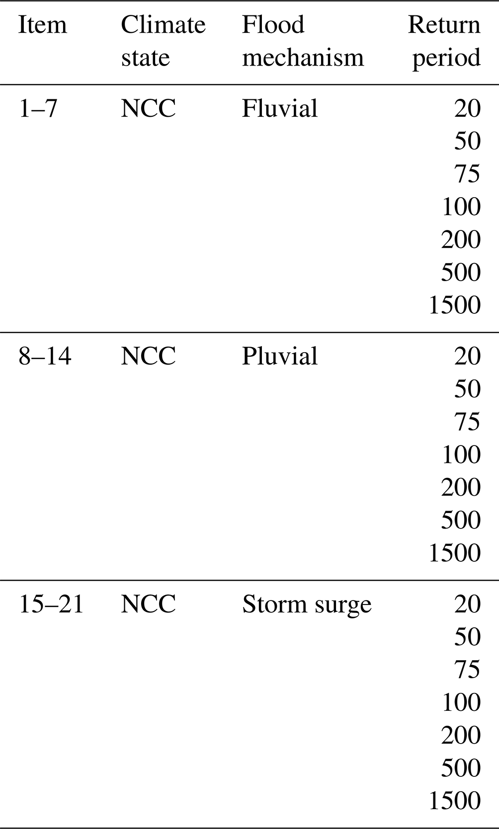
Access to the 5 m baseline and climate change flood map data was intended to pilot and explore the benefits of higher-resolution local flood hazard maps compared to the Canada-wide resolution, which is traditionally a 30 m resolution. The data were provided as a series of raster files, with each file reflecting a return period, flood mechanism, and climate state. For example, one raster file consisted of the 100-year return period, fluvial-sourced, NCC flood hazard estimation. JBA data include three main sources of flooding: (1) fluvial, (2) pluvial, and (3) storm surge flooding, each at seven different return periods (Table 1).

Table 1 Flood hazard data provided by JBA.

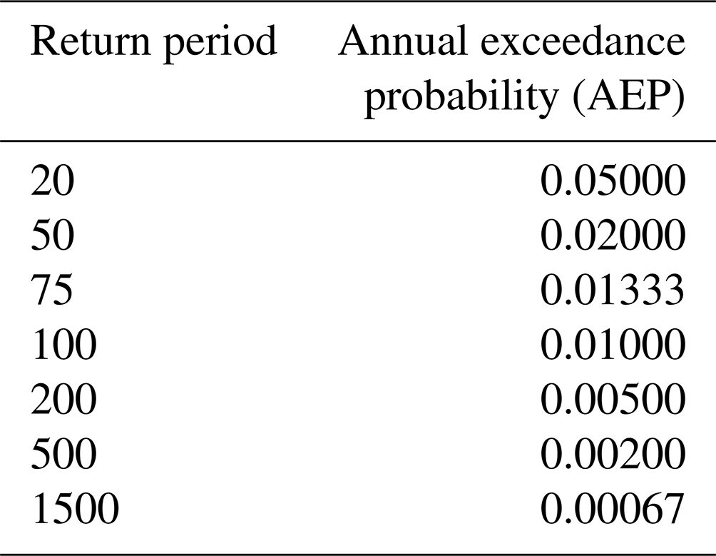
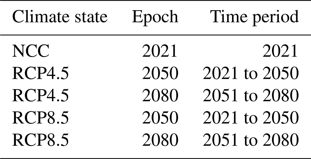
Additionally, JBA developed climate change flood hazard estimations under the RCP4.5 and RCP8.5 scenarios. Two separate time periods of assessment were used in this study: 2021 to 2050 and 2050 to 2080. This means that there was a total of five different climate scenarios, including the NCC state based on 2020–2021 modelled data and four climate-altered scenarios (Table 2).

Table 2 Climate scenarios used in the analysis.

To establish a workflow for rapidly comparing flood hazard exposure from the various JBA flood model estimates, an example exposure dataset was constructed using the open-sourced Microsoft Canadian Building Footprints (MCBF) dataset (Microsoft, 2019). This dataset contains roughly 11.8 million computer-generated building footprints across Canada using deep learning, computer vision, and artificial intelligence techniques rooted in image recognition. Buildings are usually spatially expressed as polygon or point features (Koivumäki et al., 2010), the former representing the building shape and the latter representing a single point usually inside of the structure. The benefit of building footprint data is they include more information (full shape) and are more likely to capture overlap than a single point inside of a polygon, which could miss partial flood overlap. Specifically, the MCBF dataset has been used before in flood exposure assessments (Allen et al., 2020; Buchanan et al., 2020; Huang and Wang, 2020; Porter et al., 2023), as it constitutes a readily available source of building location information across entire countries, such as Canada and the United States, and including more remote areas not mapped by other means.

A spatial computational approach is needed to determine which buildings are exposed to flooding. Techniques for estimating flood exposure to buildings inherently involve the combination of either a flood extent polygon or a flood depth raster file and a vector building dataset. For example, Allen et al. (2020) estimated the number of buildings affected by flooding by computing the intersection of each building footprint with a flood extent polygon. Buchanan et al. (2020) assumed each building polygon was exposed to flooding if it is on land at a lower elevation than a given water height, and Huang and Wang (2020) estimated exposure as buildings which fall in a floodplain boundary. Some intersections in building data with flood extent polygons may not include a depth, only a binary exposure indicator (exposed or not exposed) based on whether a building has any overlap with a flood extent. The approach used in this analysis is the summary of flood raster information at each building polygon, whereby the hazard values summarized at each building indicate an exposure, and if multiple depth values are observed, the maximum depth is selected.

MCBF data were downloaded from the Microsoft GitHub repository, specifically for British Columbia. The data were decompressed and then imported into QGIS in their raw GeoJSON file format. To extract a sample of the MCBF data relevant to the study area, the CLIP algorithm was used in the QGIS using study boundary file, as shown in Fig. 2. This resulted in 103 935 individual building polygons for the Vancouver study area.

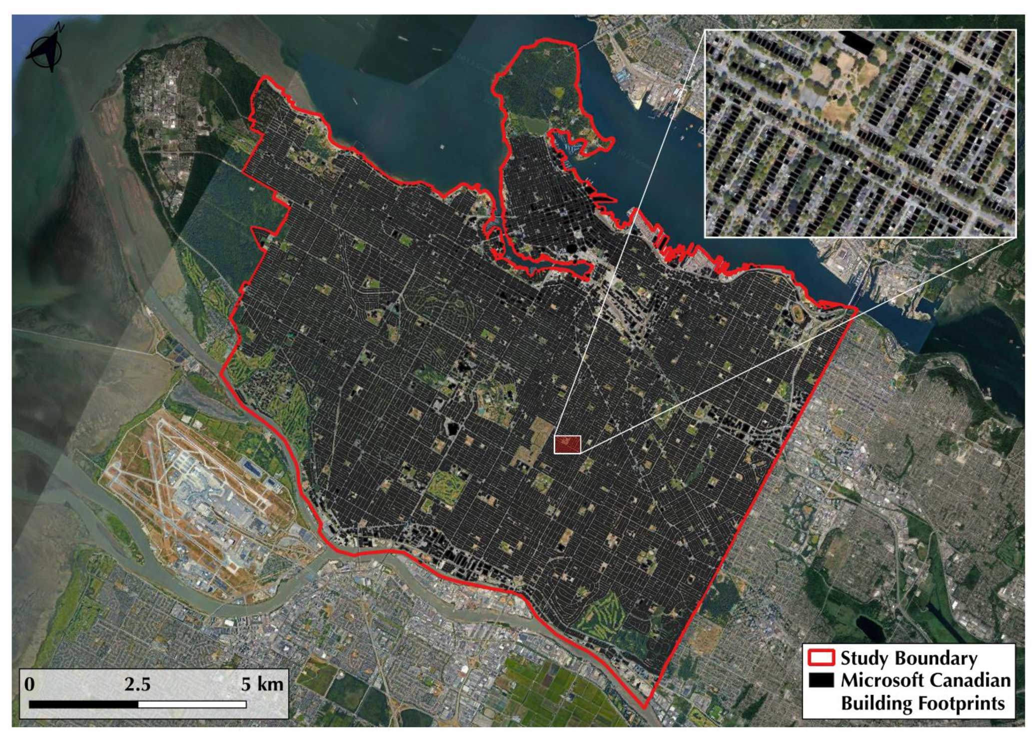
Figure 2 Study boundary delineated from a set of Statistics Canada (2019) census tracts with Microsoft (2019) Canadian Building Footprint data (n=103 935). Other map data: imagery © Google 2024, TerraMetrics, Airbus, CNES/Airbus, Maxar Technologies.

To assess flood exposure across numerous flood hazard scenarios, a Python script was developed which combined the MCBF polygon file with each of the JBA flood scenarios and return periods. Since there were five climate scenarios (CS), three flood mechanisms (FM), and seven return periods (RP), each building was assigned 105 flood depth values (21 per climate scenario):

$$\begin{array}{c}{\displaystyle }\mathrm{flood}\mathrm{hazard}\mathrm{scenarios}=N_{\mathrm{CS}}\times N_{\mathrm{FM}}\times N_{\mathrm{RP}}\\ {\displaystyle }\mathrm{flood}\mathrm{hazard}\mathrm{scenarios}=\mathrm{5}\times \mathrm{3}\times \mathrm{7}\\ {\displaystyle }\mathrm{flood}\mathrm{hazard}\mathrm{scenarios}=\mathrm{105}.\end{array}$$

To start, the MCBF building polygon dataset was opened as a geopandas file in Python. Then, a systematic loop was implemented which (1) imported one of the flood hazard files using the rasterio package and (2) computed summary statistics of the hazard files using the rasterstats zonal statistics function for each building. This procedure was repeated for each of the 105 flood hazard files, summarizing the hazard data for each building polygon. For this assessment, the maximum depth was chosen as the metric for determining exposure, such that buildings were assigned the maximum flood hazard depth for each return period intersecting a given building polygon. If any portion of a building was implicated by flood hazard data, the maximum value of flood depth was assigned.

The practice of using any building overlap is common to flood exposure estimation (Allen et al., 2020; Buchanan et al., 2020; Huang and Wang, 2020), but more information can be gleaned when also using flood depth at exposure. Since multiple flood depth measurements could occur for a given building, one must choose which to include for depth-related assessments based on the purpose of the assessment. Much like Arrighi et al. (2020), zonal statistics were computed using a series of summary statistics. However, for the purposes of this assessment, the choice of maximum flood depth at a given building was used to articulate the worst exposure possibility at a given building, which aligns with other research (Porter et al., 2023). Some authors, however, have opted to use a combination of maximum and mean flood depths to factor in outliers of the maximum depth which may be caused by erroneous cells of the terrain model (Bertsch et al., 2022). For the purposes of this assessment, the maximum depth constitutes the worst exposure scenarios for buildings where multiple depth measurements are observed and allows for the estimation of higher in-building exposure than using other summary metrics. Although there is uncertainty in the selection of a summary metric, the selection of a maximum depth is reasonable for the purposes of gauging exposure and assessing the effects of climate change.

For each climate state scenario, flood water depths were associated with each flood mechanism and return period for each address. To illustrate, Table 3 provides the different flood hazard sampling for the NCC scenario. The same information provided in Table 3 also applied to the different RCP and time scenarios illustrated in Table 2.

Table 3 Example CS–FM–RP level data at each location.

The result of this analysis was a building file that contained an associated maximum flood depth at each return period for each flood mechanism and climate state. Despite the numerous return periods available from JBA, we will continue with the remainder of the analysis using the 100-year return period to focus discussion on differentiating between sources of flooding (fluvial, pluvial, storm surge) and climate change scenarios. Future works by the authors will leverage multiple return periods to discuss the effects of climate change on different exposures at different return periods.

For this assessment, a flood depth value greater than zero indicated that a given asset was “exposed” at the corresponding return period; however, it is important to note that greater depths of water are associated with a higher likelihood of damage or loss. To account for this, three exposure metrics were computed:

1. any building with a flood depth greater than 0 m (any exposure),

2. any building with a flood depth greater than or equal to 0.3 m (moderate exposure),

3. any building with a flood depth greater than or equal to 0.6 m (severe exposure).

These thresholds were selected based on expert consultation and are also based on the 0.3 or 0.6 m freeboard which is sometimes included in provincial flood maps as an additional margin of safety in the flood elevation (National Research Council of Canada, 2021). These heights approximate 1 ft (0.3048 m) and 2 ft (0.6096 m) and were selected as general first-floor elevation (FFE) possibilities. Although there may be considerable variability in first-floor elevation across Vancouver and subjective variability in the classification of moderate or severe exposure, these values reflect a starting point for the assessment that is informed by Canadian land use information.

These different depths account for differences in first-floor elevation and doorstep height across the study area. These factors, along with other property-level considerations or broader flood defense considerations, may differentiate risk and determine whether floodwaters would enter a home and cause damage. From this assessment, an evaluation of individual return period event exposure and the suite of return period exposure was taken to determine where new flood exposure might occur because of climate change. The results of this process are described below.

4 Results

Overall, there were 103 935 building footprints identified in the study area. Of these, 16 820 (16.2 %) were identified as exposed to flooding at the 100-year return period in the NCC condition from any flood type or multiple flood types, the latter referring to buildings which may be exposed to more than one flood mechanism at the 100-year return period, such as fluvial and pluvial flooding. For moderate exposure – that which is greater than or equal to 0.3 m – there were 11 050 (10.6 %) buildings identified in the study boundary. For severe exposure – that which is greater than or equal to 0.6 m – there were 6840 (6.6 %) buildings identified in the study boundary. Table 4 provides a detailed breakdown of exposure by flood type for the NCC state in the 100-year return period.

Table 4 Breakdown of FM of exposure for the NCC state, 100-year RP flood hazard.

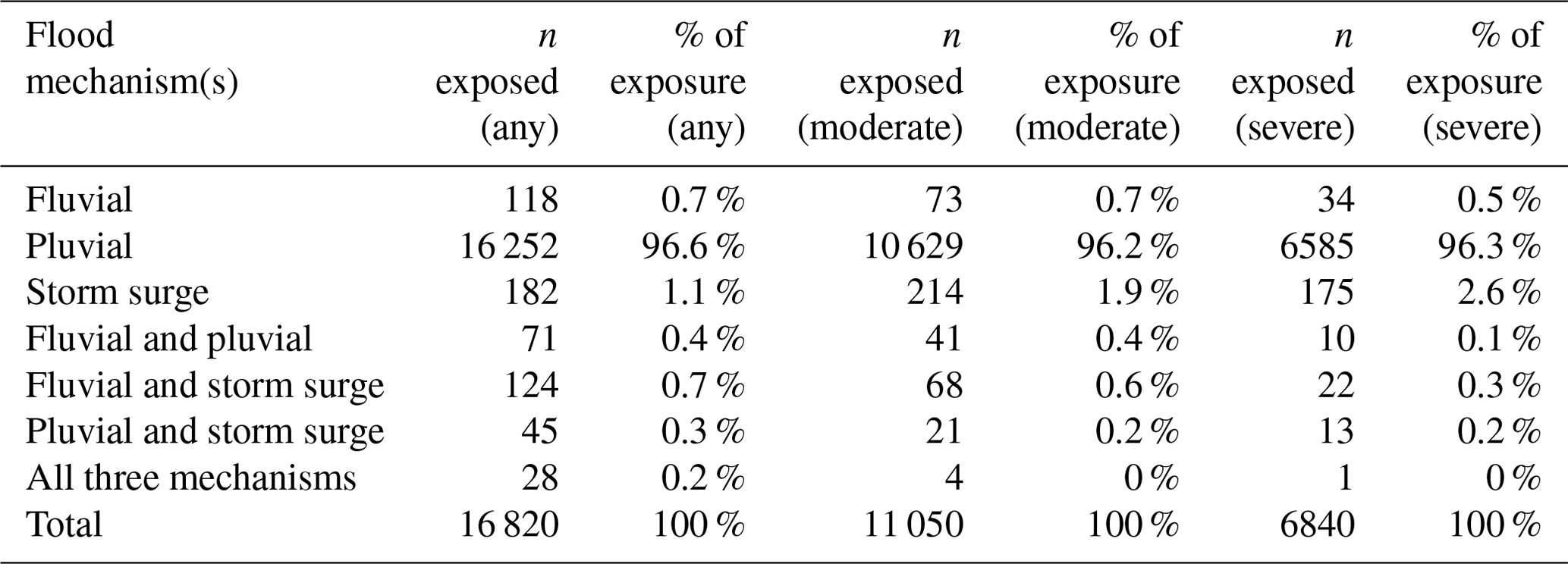
For all types of exposure in Vancouver, the overwhelming majority occurred due to pluvial flooding. Of the 16 820 buildings with any exposure to flooding, 16 252 (96.6 %) occurred from pluvial-only sourcing. The dominant exposure to pluvial flooding compared to other flood types is common partly because the geographic area is not limited to areas close to rivers or along the coast and because the drainage capacity in urban environments may be insufficient to handle the volumes of rain experienced under current and anticipated climates. The same general distribution of exposure by flood mechanism occurred across any, moderate, and severe exposure types, with pluvial being the dominant source; however, there were slightly higher proportions of severe exposure occurring from storm surge compared to estimates when using exposure at any depth.

It is worth noting that pluvial flooding involves a greater degree of uncertainty, in part due to the complexity of incorporating human-generated subsurface drainage infrastructures and waterways. For the purposes of this study, only drainage capacity assumptions were applied, and not specific details on stormwater infrastructure. Though the results indicated that pluvial flooding was the primary driver of exposure in Vancouver, this may not be true in other settings where fluvial or storm surge flooding are the drivers of exposure. Figure 3 shows the same Southlands region of Vancouver with fluvial, pluvial, and storm surge flooding, display that though all are implicated, storm surge appears to lead to more severe exposure than fluvial or pluvial flooding. This differentiation is important for determining flooding that is more likely to cause structural damage due to greater water depths.

When different climate change scenarios are factored in, flood hazard exposure can differ. Tables 5, 6, and 7 provide a detailed breakdown of the different exposures at the 100-year return period under each climate scenario for any exposure, moderate exposure, and severe exposure, respectively. For all three exposure levels, the total number of building footprints exposed increased in each climate change scenario. For example, using any exposure, the total number of buildings increased from 16 820 to 18 163 (7.98 %) for the RCP8.5 (2050) climate change state. Interestingly, this exposure is similar in magnitude for the RCP8.5 (2080) scenario, which estimated 18 156 MCBF buildings, a 7.94 % increase. Also of interest is that the total number of exposed properties at any depth decreased from RCP4.5 (2050) to RCP4.5 (2080), though both showed an estimated increase from the baseline of 16 820. It is generally accepted that RCP8.5 is more reflective of the projected climate state than RCP4.5. The same general distributions of flood exposure occurred by flood type, with pluvial-sourced flooding the dominant flood type leading to exposure in the study area of Vancouver.

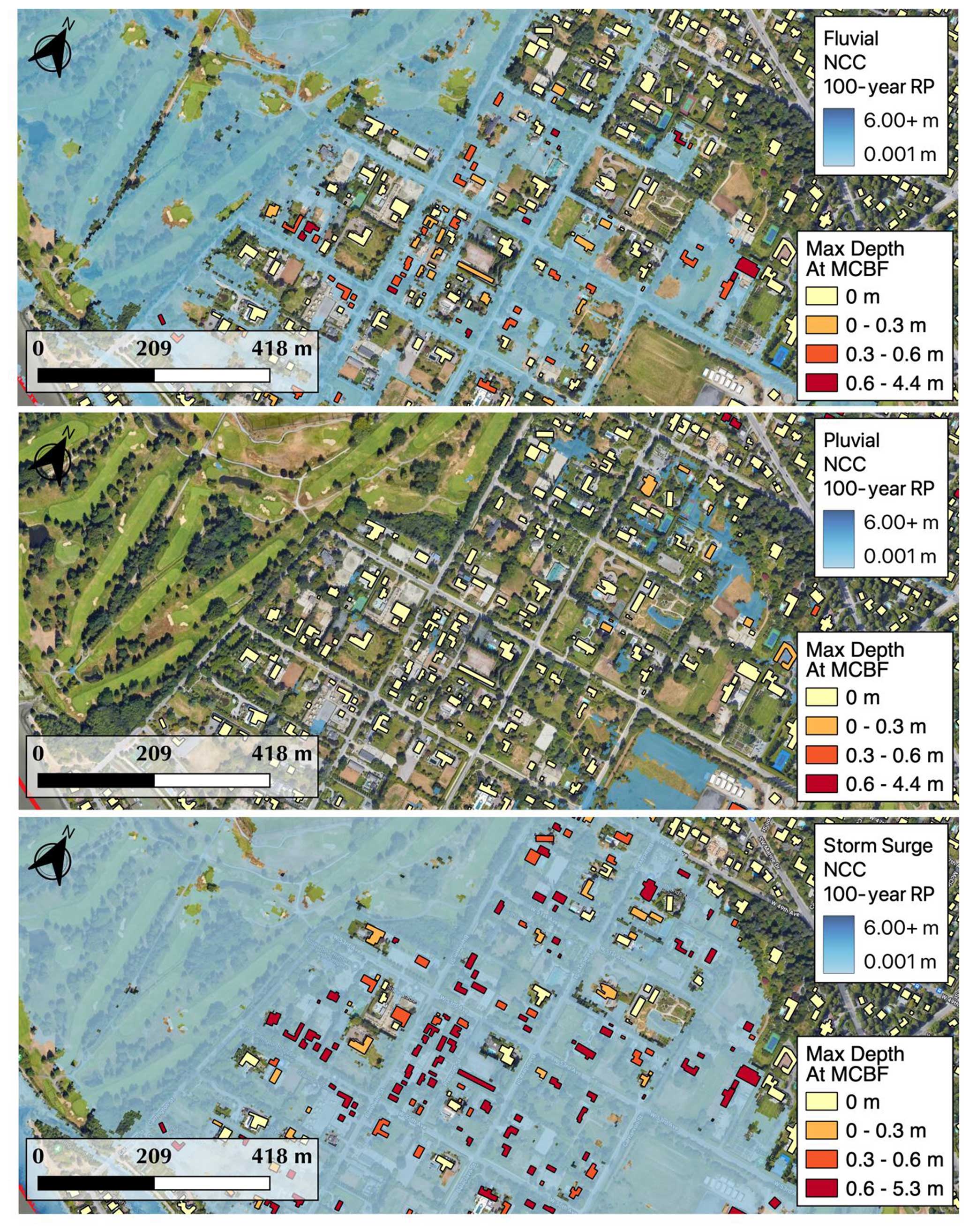
Figure 3 Flood exposure from fluvial, pluvial, and storm surge flooding for any exposure (>0 m), moderate exposure (>=0.3 m), and severe exposure (>=0.6 m) in the Southlands of Vancouver. Other map data: imagery © Google 2024, Airbus, CNES/Airbus, Maxar Technologies.

Table 5 Breakdown of any exposure by FM for the various climate states at the 100-year RP flood hazard.

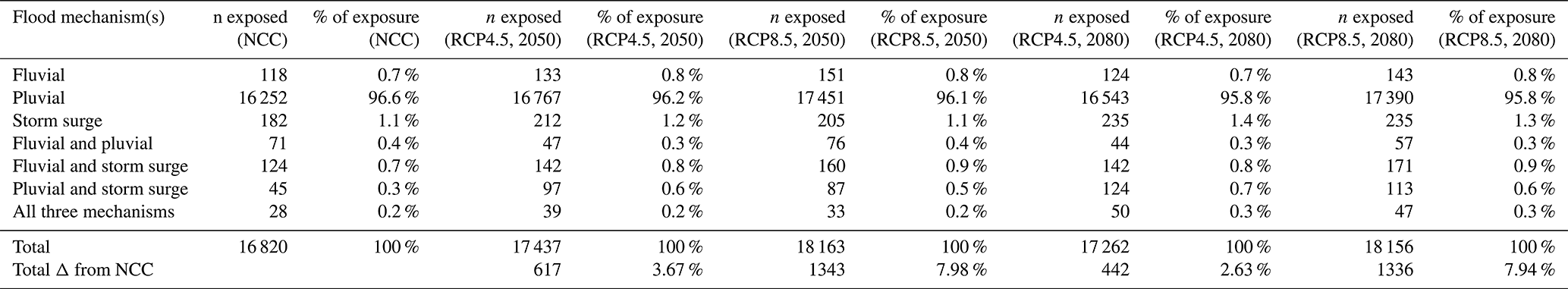
Table 6 Breakdown of moderate exposure by FM for the various climate states at the 100-year RP flood hazard.

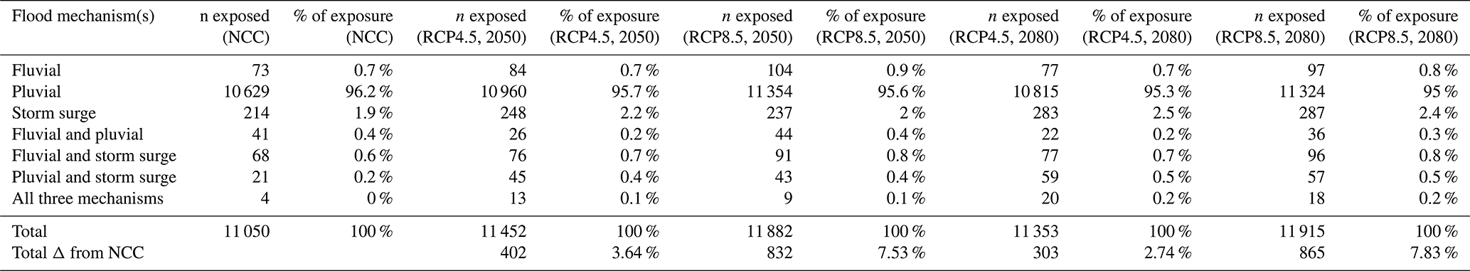
Table 7 Breakdown of severe exposure by FM for the various climate states at the 100-year RP flood hazard.

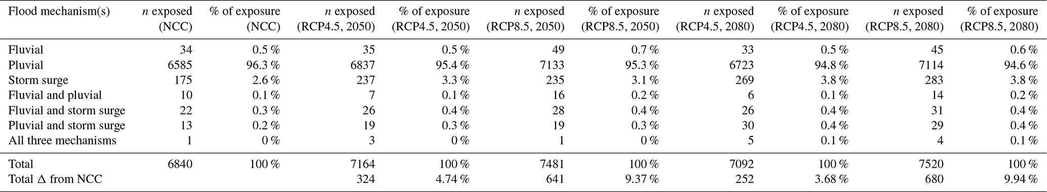
Of the 16 820 MCBF buildings considered exposed in the baseline climate scenario (Table 5), 11 050 (65.7 %) were considered to have moderate exposure (Table 6) and 6840 (40.7 %) were considered to have severe exposure (Table 7). Though pluvial flooding is the dominant source of all three exposure levels, storm surge has an increasing proportion of severe exposure in all climate change scenarios (Table 7). Although the total exposure increases for all climate scenarios, the effect of climate change seems more pronounced for severe exposure. Specifically, severe exposure increased for RCP8.5 2050 and RCP8.5 2080 between 9.3 % and 10 %, while any exposure and moderate exposure showed increases between 7.5 % and 8.0 % (Tables 5–7).

For a more detailed breakdown of the change in exposure associated with climate change projections, asset exposure was disaggregated into three general categories: (1) continued exposure, (2) new exposure, and (3) former exposure. Continued exposure refers to assets that were considered exposed to flooding at a given return period in both a non-climate-change state and given altered-climate change state and is further broken down into three sub-categories: (A) lessened exposure, (B) similar exposure, and (C) worsened exposure. New exposure refers to the assets that were not considered exposed to flooding at a given return period but are exposed under an altered climate state. Former exposure refers to the assets that were considered exposed to flooding at a given return period but were not exposed under an altered climate state. To compute each sub-category of continued exposure, the flood depths at each building were rounded to the nearest millimetre so as to avoid exceedingly small changes being classified as worsened or lessened exposures when differences are negligible.

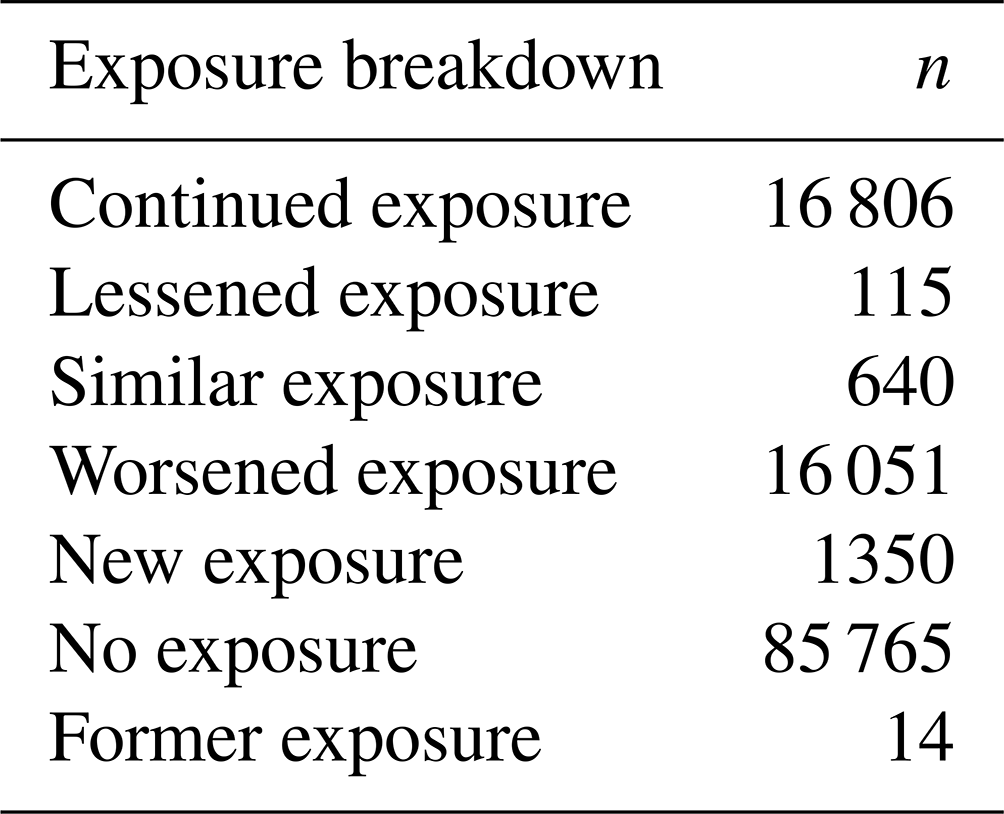
Of the 16 820 buildings that were considered exposed to any 100-year flood type and depth (i.e., fluvial, pluvial, and storm surge) under the NCC state, 16 806 continued to be exposed in the RCP8.5 2080 climate state at any depth, while 14 were no longer considered exposed. Of the continued exposure (n= 16 806), 16 051 (95.5 %) worsened in the RCP8.5 2080 climate state, 640 (3.8 %) had similar flood depths, and 115 (0.7 %) lessened in flood depth. Additionally, there were 1350 new assets exposed to flooding due to climate change. This is summarized in Table 8. The result is a total estimated exposure of 18 156 buildings for the RCP8.5 2080 climate state at any depth. An overview of this comparison is provided in Fig. 4.

Table 8 Exposure breakdown between the baseline NCC state and the RCP8.5 2080 climate state at the 100-year return period using all flood mechanisms.

For the 16 806 buildings classified as having “continued” exposure at both the NCC and RCP8.5 2080 climate states, we observed differences in the proportion of exposure that is considered moderate and severe. Of the 16 806 buildings, 11 044 (65.7 %) were considered moderate under NCC conditions, whereas 11 536 (68.6 %) were considered moderate under RCP8.5 2080 conditions, a 4.5 % (n=492) increase in the moderately exposed buildings. Severe exposure increased as well. Of the 16 806 buildings, 6837 (40.7 %) were considered severely exposed under the NCC conditions, while 7320 (43.6 %) were considered severely exposed under the RCP8.5 2080 conditions. This reflects a 7 % (n=483) increase in the severely exposed buildings.

The exposed properties were distributed all over the study site, which is to be expected from the widespread pluvial flood hazard estimation.

The overwhelming majority of these assets continued to be exposed under the RCP8.5 2080 climate state, and, due to the diffuse nature of pluvial flooding, the new exposure was scattered throughout the study site. As depicted in Fig. 4, in some cases we noted larger amounts of water leading to further exposure on the periphery of regions affected under the NCC state (inset map of Fig. 4). Such instances would be explained by more water occurring from flooding in the same areas exposed in the baseline non-climate-change state, leading to an expansion of the flood extent and greater depths of water at previously exposed buildings. Further, of the “continued” exposure, the average change in flood depth at each building was a roughly 0.04 m increase (−0.62 to 1.53 m range), although some buildings did continue to be exposed in the climate change condition but at a lesser flood depth (n=115).

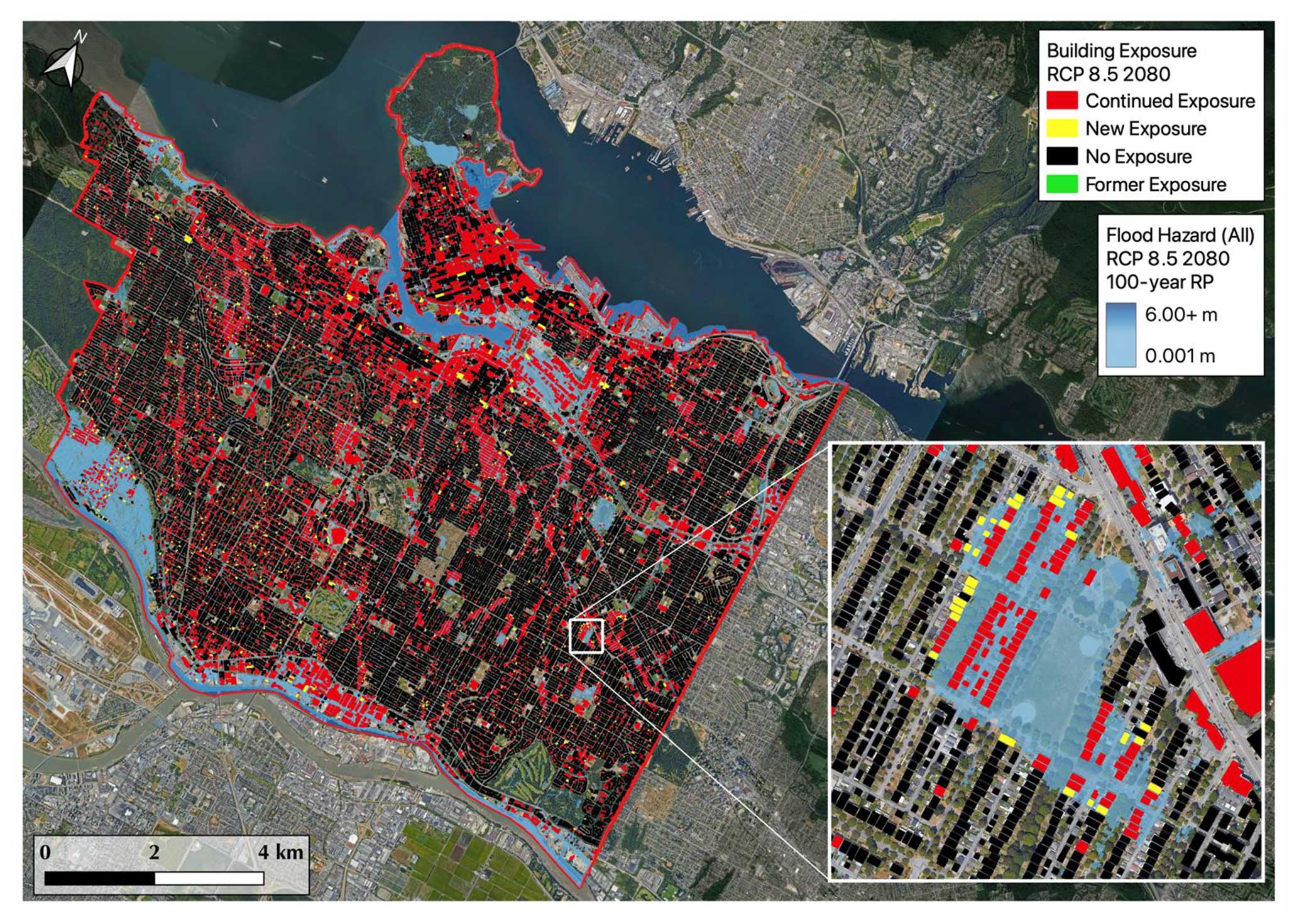
Figure 4 Overview of continued, new, and former exposure in Vancouver using the RCP8.5 2080 climate state at the 100-year return period. Study boundary from Statistics Canada (2019) census tract data. Other map data: imagery © Google 2024, TerraMetrics, Airbus, CNES/Airbus, Maxar Technologies.

Generally, we expected that most properties exposed in the NCC state would also be exposed in a climate-altered state, largely due to the expectation that all major types of flooding, including fluvial (riverine), pluvial (rainfall), and storm surge (coastal), will intensify as the climate changes (Alfieri et al., 2016; Arnell and Gosling, 2016; Hirabayashi et al., 2021; IPCC, 2019; Muis et al., 2016; Winsemius et al., 2016). Our expectation is also due to the similar assumptions embedded into the JBA climate change modules involving precipitation, temperature, and runoff. A few buildings (n=14) were determined to be exposed at the baseline non-climate-change state that were classified as non-exposed at RCP8.5 2080. For example, Fig. 5 illustrates 2 of the 14 assets classified as “former” exposure, which were considered exposed in the NCC state but not under the RCP8.5 2080 climate state at the 100-year return period. Ultimately, these were investigated individually and determined to be all pluvial-sourced flooding at shallow flood depths and almost always occurred in small pockets of disjointed pools of water. These very small artifacts in map output (e.g., where flooding in the future map was not present in the non-climate-change state) reflect the complexity in the modelling process and, for example, the way the rounding of parameters can propagate through to the end map slightly differently.

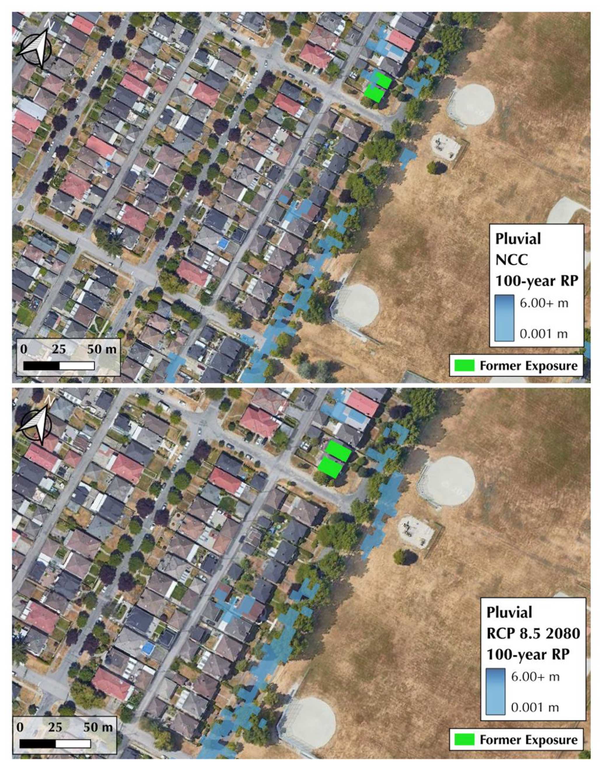
Figure 5 Example of two buildings considered exposed at the NCC state and not at RCP8.5 2080 climate state. Other map data: imagery © Google 2024, Airbus, CNES/Airbus, Maxar Technologies.

5 Discussion

The Vancouver case study demonstrates the applicability and granularity of the flood hazard mapping tool for identifying local flood exposure under a changing climate. This simplified flood hazard mapping approach was able to capture changes to flood exposure based on different climate states, flood types, and return periods. Interestingly, most of the engineered flood hazard mapping in Canada pertains to fluvial flooding (MMM Group Limited, 2014), meaning pluvial and storm surge inclusions could reflect an uncaptured source of flood risk in Vancouver by stakeholders relying on publicly available engineered maps only. Given that the results of this study indicate that pluvial flooding is the driving mechanism for anticipated flood exposure in the Vancouver area, excluding this from flood mapping could result in harmful consequences in terms of the accuracy and totality of flood hazard maps. Moreover, its absence from planning could lead to decision-making that puts vulnerable populations at higher risk of disasters by enabling further development decisions in high-risk zones, an issue that is a significant driver of current disaster risk in Canada and elsewhere.

More broadly, the higher-resolution data (5 m) constitute an improvement on >30 m resolution models being produced nationally, although local engineered mapping has typically around a 2 m resolution. By modelling climate change, this type of exposure assessment enables the mapping of changes to flood exposure for future climate states. Other benefits of this approach include its capacity to differentiate flood exposure based on the source of flooding, its scalability, and its ability to provide a generalized analysis for planners and policymakers. This approach is deemed scalable as it can be replicated in any other location in Canada, with researchers needing only to substitute the flood hazard and exposure data of interest into the established code so that the analysis can be re-run in the new setting. Although the availability of 5 m resolution and climate change data is not universal at present, JBA offers 30 m non-climate-change coverage in all areas across Canada. Although there is greater uncertainty in the pluvial flood estimation, largely because nearly all regulatory flood mapping to compare and calibrate against is fluvial and city-specific engineered drainage systems are not typically available, it constitutes a largely unmapped source of risk that could become increasingly important in urban environments.

The use of higher-resolution hazard data, climate change conditions, and multiple flood mechanisms in this analysis improves upon mapping techniques that are often low-resolution, lack climate change considerations, and are highly complex to develop (Cea and Costabile, 2022; Costabile et al., 2015; de Moel et al., 2009; Mudashiru et al., 2021; Teng et al., 2017). Moreover, this mapping approach demonstrates the relevance of physically based modelling as a modern approach to flood hazard mapping that is less costly and onerous to produce than conventional approaches. This may be especially appealing to planners and engineers who can now more effectively argue that some communities should have policies encouraging property-level flood protections.

Although the model and case study demonstrate a general and easy-to-use approach to local flood hazard mapping, they have some limitations. First, the analysis does not distinguish between building types. When reviewing Fig. 4 more closely, some structures were not identified as buildings based on the exposure dataset. Most of these structures are assumed to be sheds, but their exposure is still relevant. While this represents a limitation of the MCBF data, the use of these data in this model is a strength as well. This limitation is a product of the MCBF data and its coding. In many parts of the world, modelling flood exposure is limited by poor or even non-existent exposure datasets, such that assumptions must be made by scientists regarding population density. Here, the produced flood hazard maps show that despite some limitations within the datasets used, the overall quality of the model remains high.

Second, this model used a constant-exposure dataset based on MCBF (2019) building data. Conditions in 2050 and 2080 would also include more buildings and more exposure, which can constitute another considerable source of additional flood risk. It is anticipated that future development will lead to higher risks under future climate conditions because of the anticipated added density and number of buildings that will be exposed to flooding. For this analysis, exposure was held constant while flood hazard was modified to different climate change scenarios. Future research could consider the influence of new development on additional flood risk.

Third, this method for flood hazard mapping identifies buildings using an estimated polygon from the source data, but it does not account for building information such as building type (residential, commercial, industrial, etc.). This approach makes it difficult to differentiate flood exposure by land use and classification or for other relevant characteristics. Though there are inherent inaccuracies and a recency problem within the dataset – which was released in 2019 – the general flood exposure approach was the focus of this paper.

Finally, the produced flood hazard maps using the model presented here are considered by industry standards to be of a higher resolution than most other models, given that most large-scale maps are produced at 30 m or lower resolution. Local flood models that use physical methods to identify flood exposure could further improve the precision of these results by presenting flood exposure at an even finer scale (e.g., at a 1 or 2 m resolution). This becomes computationally challenging, especially if the spatial extent of the area grows from a single city to a provincial or even national scale, to offer consistency. Further, comparisons and validation of the flood hazard data against local engineered mapping or past flood events could reveal the hazard accuracy for known events or for on-the-ground results in Vancouver. The strengths of this approach, however, are a reasonable trade-off since this efficient flood hazard mapping approach nevertheless produces visual outputs that would be valuable for future land use planning, emergency management, policymaking, and risk awareness. Additionally, the approach may be appealing to smaller municipalities that lack resources to pursue higher-resolution modelling.

Validation of the model results is needed to rectify some of these issues. For example, a manual inspection of structures throughout the study area and comparing the results of this model against others that have higher and lower resolutions would allow us to monitor the overall accuracy of the findings. Like many other 2D hydrologic models, the JBA model makes spatial and temporal assumptions on the heterogeneous properties of the local environment (see Abbaszadeh et al., 2022; Anees et al., 2017). These assumptions are a source of uncertainty that need to be tested and calibrated by investigating the effects of model inputs (Willis et al., 2019). In the absence of any validating experiments, these maps should be viewed through a cautionary lens. Moreover, this model identifies changes to exposure due to climate change but does not consider changing socioeconomic characteristics of the area or economic consequences of flooding, nor does it include existing drainage or stormwater storage capacity, which may impact the results. These are areas requiring further research.

6 Conclusions

The acceleration of flood risk caused by climate change and expanding development in flood-prone areas requires local flood hazard maps that will enable governments, non-governmental organizations, and others to plan and implement interventions that will protect assets and populations. However, flood hazard maps often fail to account for climate change, are developed through highly technical methodologies, depict exposure to only one source of flooding, and have a coarse resolution. Leading scholarship has suggested that simplified mapping approaches are needed to overcome these weaknesses while permitting practical use by non-experts.

This paper presented a simple modelling approach to produce local flood hazard maps using a moderate 5 m resolution based on JBA Risk Management's 5 m Baseline and Climate Change Flood Map Data for Canada. In using these data, we demonstrated an empirical approach to local flood hazard mapping that produces generalizable flood exposure information. The approach can model changes to flood exposure based on the flood type, climate change projections, and return periods. This is novel to flood hazard mapping because of its scalability and its ability to capture climate change and pluvial flood exposure. This is the first study that maps Vancouver's current exposure to fluvial, pluvial, and coastal flooding at a 5 m resolution based on climate change information. While other models, like First Street Foundation, FLO-2D, and Fathom, do provide physically based solutions to mapping flood exposure across large geographic areas at a fairly high resolution, no such models exist in Canada. This represents a significant gap in geographic coverage for a country that experiences a high volume of floods annually. Moreover, as the most widely used model in the Canadian insurance market, this study demonstrates the utility of the JBA model in providing comprehensive coverage for fluvial, pluvial, and coastal flooding. While certain limitations do exist – including the inability to differentiate exposure based on building type (e.g., residential versus commercial) – the approach enables local planners, policymakers, and other stakeholders to pursue flood risk management strategies.

Further research is needed to validate the findings of the current model and its replicability in other jurisdictions. Comparing the resulting local flood hazard map with maps produced using other methodologies – including physical and empirical models – and against historical flood events would allow us to validate the findings even further. Validating climate change hazard estimation remains a challenge due to the uncertainty surrounding climate change effects; however, this model constitutes a step forward in the use of forward-looking flood hazard and exposure estimation.