the Creative Commons Attribution 4.0 License.
the Creative Commons Attribution 4.0 License.
 | 14 Feb 2024
CRHyME (Climatic Rainfall Hydrogeological Modelling Experiment): a new model for geo-hydrological hazard assessment at the basin scale
Andrea Abbate
Leonardo Mancusi
Francesco Apadula
Antonella Frigerio
Monica Papini
Laura Longoni
This work presents the new model called CRHyME (Climatic Rainfall Hydrogeological Modelling Experiment), a tool for geo-hydrological hazard evaluation. CRHyME is a physically based and spatially distributed model written in the Python language that represents an extension of the classic hydrological models working at the basin scale. CRHyME's main focus consists of simulating rainfall-induced geo-hydrological instabilities such as shallow landslides, debris flows, catchment erosion and sediment transport into a river. These phenomena are conventionally decoupled from a hydrological routine, while in CRHyME they are simultaneously and quantitatively evaluated within the same code through a multi-hazard approach.
CRHyME is applied within some case studies across northern Italy. Among these, the Caldone catchment, a well-monitored basin of 27 km2 located near the city of Lecco (Lombardy), was considered for the calibration of solid-transport routine testing, as well as the spatial-scale dependence related to digital terrain resolution. CRHyME was applied across larger basins of the Valtellina (Alps) and Emilia (Apennines) areas (∼2600 km2) which have experienced severe geo-hydrological episodes triggered by heavy precipitation in the recent past. CRHyME's validation has been assessed through NSE (Nash–Sutcliffe efficiency) and RMSE (root mean square error) hydrological-error metrics, while for landslides the ROC (receiver operating characteristic) methodology was applied. CRHyME has been able to reconstruct the river discharge at the reference hydrometric stations located at the outlets of the basins to estimate the sediment yield at some hydropower reservoirs chosen as a reference and to individuate the location and the triggering conditions of shallow landslides and debris flows. The good performance of CRHyME was reached, assuring the stability of the code and a rather fast computation and maintaining the numerical conservativity of water and sediment balances. CRHyME has shown itself to be a suitable tool for the quantification of the geo-hydrological process and thus useful for civil-protection multi-hazard assessment.
- Article
(7660 KB) - Full-text XML
- BibTeX
- EndNote


Natural disasters are a critical issue in terms of economic losses and casualties (ISPRA, 2018). For 2020 alone, the worldwide losses related to geohazard were quantified as USD 210 billion and 8200 victims (Munich Re, 2021). Among the natural disasters, the events linked to geo-hydrological phenomena, such as floods and landslides, certainly play a significant role. Floods and landslides represent serious geo-hydrological hazards in mountain environments (Gariano and Guzzetti, 2016). Among them, shallow landslides, debris flow failures and soil erosion are controlled by rainfall-triggering events of varying intensity and duration (Abbate et al., 2021a), while sediment transport is a hydrologically driven process occurring at the catchment scale (Brambilla et al., 2020; Papini et al., 2017; Longoni et al., 2016; Ballio et al., 2010). In Italy, a total area of 50 117 km2, corresponding to 16.6 % of the national territory, is affected by high or very high landslide hazards and/or by a medium hydraulic hazard (ISPRA, 2018). In 2021, the number of victims of landslide and flood events was 5 and the evacuated people were around 1000 (CNR and IRPI, 2021). Northern Italy has the highest mortality rate caused by landslides and floods in the country, varying in the range of 0.034 for Emilia Romagna and 0.085 for Piedmont (number of deaths and missing people per 100 000 people in 1 year).
Geo-hydrological hazards are complex and heterogeneous phenomena, so a great effort has been made in the past to understand their dynamics (Gariano and Guzzetti, 2016; Ceriani et al., 1994; Gao et al., 2018; Kim et al., 2020). There are many studies concerning shallow-landslide dynamics in the literature, based both on laboratory and on field experiments (Guzzetti et al., 2007; Herrera, 2019; Meisina et al., 2013; Crosta et al., 2003; Iverson, 2000; Ivanov et al., 2020b), which highlighted the rainfall as the most important triggering factor. Conversely, debris flow and solid transport are primarily influenced by superficial soil water balance in terms of runoff generation through the infiltration mechanisms (Abbate et al., 2019; Jakob and Hungr, 2005; Vetsch et al., 2018). Even though the hydrological cycle is identified as the principal driver of geo-hydrological processes, a widely accepted methodology able to straightforwardly connect these hazard types and their predisposing and triggering factors is still missing (Gariano and Guzzetti, 2016; Bordoni et al., 2015).
This work will illustrate the potential of a new physically based geo-hydrological model called CRHyME (Climatic Rainfall Hydrogeological Modelling Experiment). CRHyME is an extension of a classical rainfall-runoff hydrological model where geo-morphological dynamic aspects are also simulated. From the analysis of the literature (De Vita et al., 2018; Bemporad et al., 1997; Roo et al., 1996; Schellekens et al., 2020; Angeli et al., 1998; Gleick, 1989; Sutanudjaja et al., 2018; Van Der Knijff et al., 2010; Devia et al., 2015; Moges et al., 2021), the geological and hydrological aspects have rarely been jointly taken into account within the same framework. Lots of hydrological models adopted worldwide are interested mainly in flood propagation and water balance assessment (Sutanudjaja et al., 2018), proposing a very detailed and advanced description of the hydrological cycle. However, geo-hydrological hazard interaction is hardly taken into account (Shobe et al., 2017; Strauch et al., 2018; Campforts et al., 2020), and it represents one of their main limitations. Up to now, there have been few examples that can include the triggering analysis of shallow landslide and debris flow or a solid-transport quantification (Roo et al., 1996; Gariano and Guzzetti, 2016; Alvioli et al., 2018). In the literature, some consider the erosion and solid-transport mechanisms at the watershed scale (Vetsch et al., 2018; Tangi et al., 2019; Roo et al., 1996; Papini et al., 2017), while the stability of natural slopes is generally not included. Conversely, the slope stability or debris flow analysis is computed inside dedicated models (Iverson, 2000; Scheidl and Rickenmann, 2011; Harp et al., 2006; Milledge et al., 2014; Montrasio, 2008; Takahashi, 2009) where strong hypothesis and simplification of the hydrological parameterization are adopted.
Geo-hydrological phenomena have been historically decoupled and investigated separately. To fill this gap and make them more integrated within a numerical model, some attempts were recently proposed. In this regard, CHASM (Combined Hydrology And Stability Model) (Bozzolan et al., 2020) and Landlab (Strauch et al., 2018) represent the two latest modelling frameworks that have addressed the need to start evaluating the geo-hydrological hazard and risks jointly with hydrological and climatic aspects. The new methodological approaches shown by the CHASM and Landlab models have been assessed thanks to the progressive increase in the GIS (geographical information system) data availability on a worldwide scale and thanks to the recent improvements in computer programming for environmental systems modelling. Indeed, the creation of efficient and open-source built-in functions for different language programmes, such as MATLAB, C or Python, has sped up and facilitated the implementation of self-made land surface models. These functions have already been successfully implemented by the PCR-GLOBWB 2 (Sutanudjaja et al., 2018) and wflow (Schellekens et al., 2020) models, as well as in the European hydrological model LISFLOOD (Van Der Knijff et al., 2010) and OpenLISEM (Roo et al., 1996).
Among the currently available modelling approaches and software solutions, a comprehensive multi-hazard model specifically designed for evaluating geo-hydrological threats is still needed. Geo-hydrological processes are many and happen simultaneously at a watershed scale. They are required to be modelled together to better understand their mutual influences and feedback, by trying to overcome the theoretical subdivisions that exist in the literature's methodologies. Moreover, diversified input data formats, their spatial and temporal resolution, and the scale dependency of geo-hydrological simulation (Devia et al., 2015; Moges et al., 2021) represent real challenges to be carefully addressed to not undermine the applicability of these integrated models. Under these premises, the main motivations aimed at the construction of the new CRHyME code are presented here:
-
build an integrated but versatile model for simulating rainfall-induced geo-hydrological processes (flood, erosion, sediment transport and shallow-landslide triggering);
-
allow for fast and efficient calculations within a spatially distributed model designed to operate at the catchment scale without constraints on spatial and temporal input data resolution;
-
implement code inside a robust framework, using open-source Python libraries which enable fast coding and easy submodule modifications/integrations;
-
address code compatibility for assimilating input data from open-source datasets available at a worldwide scale, permitting a simulation reproducibly in any worldwide catchment.
Starting from these considerations and taking inspiration from analogue models cited before, CRHyME (Fig. 1) was developed to try to improve overall geo-hydrological modelling, filling the existing gaps and issues. This paper presents the key features and applications of the code. Structure and constitutive equations are reported in the “Material and methods” section. Then some case studies developed across the Italian territory were considered for the calibration and validation of the new model. In the Results section the main outcomes of CRHyME applications are reported, and they are extensively commented on within the Discussion and Conclusion sections.

In this section, the CRHyME model's main features, the submodule structure and their constitutive equations, the input dataset required for its initialization, and a presentation of calibration and validation case studies are illustrated.
2.1 Key model features
CRHyME aims to model together rainfall-induced hydrological and geological processes at the catchment scale, e.g. floods and landslides. In CRHyME these processes are evaluated simultaneously within the hydrological routine: the bed-load sediment transport has been described considering the erosion potential method (EPM) for simulating erosion sources (Longoni et al., 2016; Brambilla et al., 2020; Milanesi et al., 2015; Ivanov et al., 2020a) and the stream power laws for defining the transport capacity of the rivers (Vetsch et al., 2018); the shallow-landslide failure assessment was carried out considering four infinite-slope stability models by Iverson (2000), Montrasio (2008), Harp et al. (2006) and Milledge et al. (2014); and the debris flows behave intermediately among floods and landslides, and their stability assessment was evaluated through the theory proposed by Takahashi (2009), Theule (2012), and Jakob and Jordan (2001).
The CRHyME's code architecture is partially inherited from the PCR-GLOBWB 2 model (Sutanudjaja et al., 2018). This model is characterized by a well-organized framework that could guarantee the robustness and stability of the code, fast modelling and reduced time consumption thanks to embedded function parallelization, and no constraints on the spatial and temporal resolution of the input data. The PCR-GLOBWB 2 engine is based on PCRaster libraries (Karssenberg et al., 2010; Pebesma et al., 2007). The PCRaster Python libraries offer a series of standard functions for hydrological processing on calculation grids which can be easily “called” via Python scripts to perform individual operations. CRHyME's framework is organized within a modular structure which enables easier single-model updating and facilitates the introduction of new features. The Python programming language is open-source, and its flexibility permits the fast management of GIS databases which are essential for computing geo-hydrological hazard simulations over large domains.
2.2 Model structure
The CRHyME model is composed of a series of modules that run successively in a time loop as represented in Fig. 2. The simulations are initialized from a pre-compiled .INI file (see Appendix A), where all the settings and input data are specified (see Appendix B). The first six modules evaluate the hydrological cycle and constitute the hydrological module. A novel aspect of CRHyME is the landslide module, where slope instability conditions and sediment transport dynamics are simulated considering the computed soil moisture and the runoff, respectively. The modules included in the code are the following:
-
CLIMA elaborates precipitation and temperature data from reanalysis and climate datasets, using the NetCDF (Network Common Data Form, .netcdf) format (Bonanno et al., 2019; Sutanudjaja et al., 2018);
-
METEO elaborates precipitation and temperature data from ground-based weather stations using the PCRaster standard format (.tss) (Karssenberg et al., 2010) for data series and calculates the evapotranspiration;
-
INTERCEPTION excludes the canopy interception from the net precipitation and computes the snow dynamic;
-
LANDSURFACE evaluates the water balance in the superficial soil, giving information about runoff, soil moisture and percolation losses;
-
GROUNDWATER evaluates the water balance in the groundwater layer;
-
ROUTING calculates the runoff routing across the watershed;
-
LANDSLIDE identifies the triggering conditions for landslides and debris flows and calculates erosion and bed-load sediment transport in rivers.
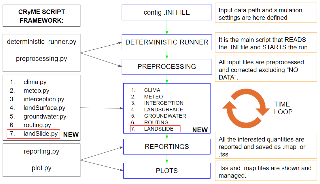
Figure 2Framework of the CRHyME model. The main Python scripts are listed, explaining their functionality and their link with the other parts of the code. For further details see Appendix A and Appendix B.
2.2.1 Model initialization
A fundamental starting point for CRHyME's code initialization consists of the choice of a suitable digital elevation model (DEM). From the DEM all the essential data listed in the .INI file are derived: clone.map is a 0–1 mask that defines the computational domain, and ldd.map is the local drain direction map (Karssenberg et al., 2010; Pebesma et al., 2007). In CRHyME, the HydroSHEDS DEM (Hydrological data and maps based on SHuttle Elevation Derivatives at multiple Scales, https://www.hydrosheds.org, last access: 1 November 2023) (Lehner et al., 2008) was taken as a reference. The HydroSHEDS DEM is designed specifically for hydrological models and has been already preprocessed to guarantee the flow connectivity of the river network (hydrologically conditioned). Its spatial resolution is about 3 s degree, which corresponds approximately to about 90 m at the Equator, and it was retained sufficiently accurately for medium-scale catchment analysis. Using the built-in PCRaster functions, the flow accumulation, the slope, the curvature and the slope-aspect data were reconstructed immediately from HydroSHEDS DEM. In addition to these morphological data, other informative layers are required for geo-hydrological assessment:
-
the CORINE Land Cover data (https://land.copernicus.eu, last access: 1 November 2023) (Girard et al., 2018) form the European inventory of land cover that was considered for defining vegetation interception and soil infiltration coefficients, spatial evapotranspiration flux, and root cohesion for landslide stability;
-
the SoilGrids data at 250 m resolution from the global ISRIC (International Soil Reference and Information Centre) database of World Soil Information (https://maps.isric.org/, last access: 1 November 2023) (Hengl et al., 2017) were considered for assessing soil physical properties such as depth and soil composition which are implemented in infiltration, percolation, erosion and landslide stability routines;
-
the hydraulic properties of soils, such as permeability and porosity, from the European Soil Data Centre (ESDAC) database (https://esdac.jrc.ec.europa.eu/, last access: 1 November 2023) and other worldwide repositories (Tóth et al., 2017; Ross et al., 2018; Huscroft et al., 2018), were considered for assessing superficial and groundwater hydrological balance.
The datasets described here are freely available for the entire European area, but analogies could be found for other continents. Since they are provided with an open-source licence, they have been implemented without restrictions. This choice aims to extend and generalize the reproducibility of CRHyME's simulations in any worldwide catchment as much as possible while avoiding any constraint on territorial input data. Moreover, these databases provide free Web Feature Service (WFS) and Web Coverage Service (WCS) services, allowing for downloading them more easily and speeding up CRHyME initialization.
Temperature and rainfall data required by simulations were gathered from ground-based meteorological stations (Rete Monitoraggio ARPA Lombardia, 2023; Rete Monitoraggio ARPA Emilia-Romagna, 2023; ARPA: Agenzia Regionale per la Protezione Ambientale, Regional Agency for the Protection of the Environment) and locally available reanalysis databases (Bonanno et al., 2019). Temperature fields were built by combining the data series at each time step, estimating the regression coefficient with respect to the station elevation and then using the DEM information to calculate the temperature distribution (Daly et al., 1997; Chow et al., 1988). For rain gauge precipitation, a simple IDW (inverse distance weight) interpolator was implemented with a distance exponent equal to 2, while for rainfall data in the reanalysis data, a simple nearest-neighbour algorithm has been adopted to downscale the precipitation field at DEM resolution (Daly et al., 1997; Chow et al., 1988; Abbate et al., 2021b; Terzago et al., 2018). CRHyME's time step required for completing a single loop of all internal modules (Fig. 2) was assumed to be equal to the meteorological forcings time step and could vary from a minimum of 5 min up to a maximum of 1 d. In this current work, the time step selected for CRHyME's computations is 1 d.
2.2.2 Hydrological modules and equations
The hydrological modules (Figs. 2 and 3, from 1 to 6) evaluate the processes of transformation inflows–outflows using input maps of weather forcings consisting of precipitation P [mm per time step] and average, maximum and minimum temperature T [∘C]. In CRHyME, each cell of the terrain domain is considered to be a tank that communicates in cascade with the others following the downstream river network (Brambilla et al., 2020; Roo et al., 1996; Sutanudjaja et al., 2018). Hydrological balance is schematized considering four imaginary layers where water can be temporarily stored.
-
Snow storage. In Eq. (1), the snow balance is assessed by the quantity hsnow(t) [mm].
-
Superficial soil storage. In Eqs. (2) and (3), soil infiltration is computed and the superficial soil balance is assessed by the variable hsoilwater(t) [mm].
-
Groundwater soil storage. In Eq. (5), the groundwater balance is assessed by the quantity hgroundwater(t) [mm].
-
Runoff storage. In Eq. (6), the runoff generated by an excess of infiltration and exfiltration is routed across the catchment and described by the variable hrunoff(t) [mm].
The superficial soil storage is the core of hydrological balance assessment where all the water mass fluxes [mm per time step] are exchanged between atmosphere and terrain. Balances are schematized by Eqs. (1)–(3).
-
The infiltration balance in Eq. (2) establishes the net water volume I(t) that enters the soil. From precipitation P(t) the net precipitation arriving at the soil interface Pn(t) is evaluated by subtracting the rainfall intercepted by tree leaves, i.e. canopy interceptions CI(t) (Li et al., 2017; Nazari et al., 2019). When the temperature T is <0 ∘C, all the precipitation is stored as snowpack hsnow(t) (Eq. 1) and released afterwards as snowmelt contribution Sml(t) when the temperature increases above 0 ∘C following a degree-day approach (Chow et al., 1988; Cazorzi and Dalla Fontana, 1996). I(t) is estimated directly using the common infiltration methods proposed by Horton (exponential decreasing infiltration with time) and SCS-CN (Soil Conservation Service curve number; Chow et al., 1988; Chen and Young, 2006; Mishra et al., 2003; Morbidelli et al., 2018; Ravi et al., 1998; Smith and Parlange, 1978; Ross et al., 2018), and the runoff generated by an excess of precipitation at the surface R(t) is obtained by the difference in Pn(t)−I(t).
-
The superficial soil moisture balance in Eq. (3) permits evaluating the quantity Sm(t), which is expressed as a dimensionless ratio between hsoilwater(t) [mm] and the product of terrain porosity n and the superficial soil depth (depthSoil). Porosity and the superficial soil depth are determined from the databases of Tóth et al. (2017), Ross et al. (2018), Huscroft et al. (2018) and Hengl et al. (2017), respectively. The other terms of the water balance are the following.
-
ETc(t) evapotranspiration losses are determined according to the Hargreaves and Penman–Monteith formulations suggested by FAO (Food and Agriculture Organization of the United Nations) guidelines (Raziei and Pereira, 2013; Allan et al., 1998).
-
Lper(t) percolation losses are part of the volume that goes to the groundwater layer, evaluated as a function of the soil water balance in unsaturated conditions using Van Genuchten's functions and parameters (Tian et al., 2016; Van Genuchten, 1980; Daly et al., 2017; Groenendyk et al., 2015; Vitvar et al., 2002; Jackson et al., 2014; Klaus and Jackson, 2018).
-
Exfiltration Ex(t) is the leakage of water on the surface that occurs after the complete saturation of the superficial soil storage (ponding).
-
Fsub(t) [m3 s−1] is the subsurface lateral fluxes generated inside the superficial soil layer through the Dupuit approximation of the Darcy law for water filtration in soils. Here, a correction of the saturated permeability Ks [m s−1] considering the relative permeability Kr [–] caused by the partial saturation conditions has been included in the formula (Van Genuchten, 1980). Δx and Δy represent the cell dimensions [m]. The resultant advection term has been converted [mm per time step] to be consistent with other measurement units.
-
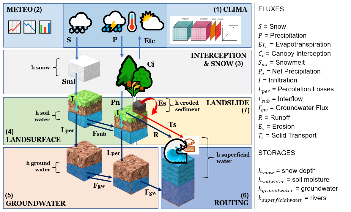
Figure 3Scheme of the soil water and sediment balances and related mass fluxes implemented in CRHyME. Fluxes and storage variables constituting the model are listed with their symbols.
The groundwater reservoir depth (depthGW) has been modelled considering the spatial distribution described in Eq. (4) (Fan et al., 2007; de Graaf et al., 2015; Pelletier et al., 2016). According to these studies, as the superficial slope increases, the aquifer depth is reduced until it reaches the minimum value of 0 m, corresponding to the condition of complete absence.
In Eq. (4) the slope is expressed as a tangent to the angle of inclination of the surface, while a and b represent coefficients that are distinguished according to the depths of interest: where the depth of the bedrock is supposed to be low (<10 m, superficial bedrock) and the suggested parameters are a=20 and b=125 or a=120 and b=150 if the bedrock depth is significant (>10 m, deep regolith). In CRHyME an intermediate condition has been adopted between superficial bedrock and deep regolith; therefore the parameters adopted are the following: a=200 and b=125. This approximation has appeared sufficiently accurate concerning the fact that currently available data on groundwater aquifer depth and hydrogeological parameters are rather approximated, uncertain and of low resolution (Kobierska et al., 2015; Zomlot et al., 2015; Hayashi, 2020; Huscroft et al., 2018).
The groundwater table is generated by the percolated water Lper(t) coming from the upper layer Eq. (5). The groundwater lateral flow FGW(t) [m3 s−1] is then calculated using the Dupuit approximation according to which the filtration rate is given by the product of hydraulic permeability for the tangent of the slope of the impermeable substrate, supposed parallel to the slope (Klaus and Jackson, 2018; Anderson, 2005; Bresciani et al., 2014). The resultant advection term has been converted [mm per time step]. Groundwater exfiltration ExGW(t) is the term that describes the leakage of water after the complete saturation of the groundwater storage, simulating the water springs.
Superficial runoff is defined as the sum of R(t), Ex(t) and ExGW(t), and it is stored in hrunoff(t) in Eq. (6). hrunoff(t) is propagated across the overland surface along the lines of maximum slope and inside the river network using two possible methods available in PCRaster libraries (kinematic and dynamic) that are deputed for the flow routing process (Chow et al., 1988; Lee and Pin Chun, 2012; Collischonn et al., 2017; Bancheri et al., 2020). Fkin-dyn(t) flux [m3 s−1] is derived from the simplification of de Saint-Venant's one-dimensional equations of motion. The kinematic algorithm is generally applied in sections where the slopes are accentuated so it is possible to approximate the hydraulic gradient with the slope of the channel (Chow et al., 1988). The dynamic algorithm instead introduces further terms that allow for a better simulation of the outflow in correspondence to the flat areas when the other terms of the de Saint-Venant equation are no longer negligible (Chow et al., 1988) but require precise information about the geometry of rivers sections to carry out the flood wave propagation (Karssenberg et al., 2010). The resultant advection term has been converted [mm per time step].
2.2.3 Geo-hydrological module and equations
To study geo-hydrological instability, it is of paramount importance to analyse the triggering causes of landslides and the dynamic of erosion and sediment transport processes (Guzzetti et al., 2005; Remondo et al., 2005; Montrasio and Valentino, 2016; Bovolo and Bathurst, 2012). In the following paragraphs, the landslide module features included in CRHyME are described (Fig. 3, no. 7).
Stability models for shallow landslides and debris flows
Shallow-landslide triggering is strongly correlated with meteorological and climatic forcing (Abbate et al., 2021a). The abrupt modifications of the local hydrology with the alternation of dry and wet conditions of soil induced by precipitation are responsible for undermining the stability of the slopes (Iverson, 2000; Chen and Young, 2006). The four stability models included in CRHyME are briefly described here: (1) the Iverson model (Iverson, 2000), Eq. (7); (2) the Harp model (Harp et al., 2006), Eq. (8); (3) the Milledge model (Milledge et al., 2014), Eq. (9); and (4) the SLIP model (Montrasio, 2008; Montrasio and Valentino, 2016), Eq. (10). In slope stability analysis, the limit equilibrium method based on the Mohr–Coulomb criterion is usually adopted to calculate slope stability. The one-dimensional theory considers the hypothesis of an infinitely extended slope characterized by soil thickness Z [m], plane inclination α [∘], and saturated soil γs and water γw specific weight [kN m−3]. The slope stability is evaluated by the factor of safety (FS), defined as the ratio between the resistant forces due to the friction and the mobilizing forces due to the weight component parallel to the slope. In CRHyME, the one-dimensional model was implemented by imagining each cell as a slope element for which the value of the factor of safety FS is calculated. According to the principle of effective stress, as the soil moisture increases, normal efforts are reduced by an aliquot equal to the pressure generated by the water itself (Iverson, 2000).
The key parameters of the Iverson (Iverson, 2000) Eq. (7) and Harp (Harp et al., 2006) models Eq. (8) are essentially threefold: the friction angle φ [∘] and the cohesion of the soil c [kPa], which are a function of the terrain granulometry, and the superficial soil moisture Sm(t) [m]. Inside the Iverson model, the soil moisture influence is described through the groundwater pressure head of the local aquifer [kPa], while inside the Harp model it is described by the dimensionless variable , comprised between 0 (completely dry) and 1 (completely wet). The Milledge model (Milledge et al., 2014) in Eq. (9) considers not only the friction effects along the sliding surface Frb [N] but also the shear resistance along the two parallel and vertical side walls Frl [N], the passive force of the upstream terrain Fdu [N], the active force of the valley terrain Frd [N], and the mobilizing force due to the terrain weight Fdc [N]. In the SLIP model (Montrasio, 2008; Montrasio and Valentino, 2016) shown in Eq. (10) the terms are expressed in newtons: N is the normal component of the weight as a function of porosity n and soil moisture Sm(t), C is the cohesion term, W is the slope parallel component of the weight as a function of porosity n and soil moisture Sm(t), and F is the term that expresses the seepage forces that are related to the presence of the temporary water table. Since slopes are vegetated, two other factors should be included: the additional cohesion of the root system of trees and the additional weight of plant biomass (Cislaghi et al., 2017; Yu et al., 2018; Rahardjo et al., 2014). In fact, in the absence of root cohesion, several slope areas would be perpetually in conditions of instability with FS < 1. The addition of root cohesion, varying between 1–10 kPa, depending on the tree species and the type of land use, was included in the stability evaluation (further details in Abbate and Mancusi, 2021a).
A debris flow represents movements of mass that are often triggered on steep slopes and travel long distances reaching the fan close to the watershed outlet (Takahashi, 2009). Debris flows are classified as landslides, although they are among the more fluid types of landslides (Iverson et al., 1997). Therefore, solid concentration within the saturated deposit and the presence of superficial water flowing above are the key parameters for assessing the triggering condition. As can be appreciated by Eqs. (11) and (12), at least two criteria are included. The first one is derived from the theory of infinite-slope stability, where the solid concentration parameter C* is included as the principal triggering factor. The solid concentration C* is the grain concentration by volume in the static debris bed and can be expressed by the ratio between the soil amount [m3] to the sum of the soil amount [m3] and soil water volume [m3]. Increasing the local water volume, the solid concentration starts to progressively reduce. The first criterion in Eq. (11) requires the indication of soil density σ [kg m−3]; water density ρ [kg m−3]; the surface runoff height hrunoff [m]; and the parameter adf that can be assumed equal to the representative diameter of the soil deposit, such as D50 [m]. The second criterion in Eq. (12) considers that specific superficial runoff discharge or [m2 s−1], where B is the channel width, flowing above the debris deposit, satisfies the threshold condition of ≥ 2 for the non-dimensional water discharge q* [–], where g is gravity acceleration [m s−2]. If these criteria are satisfied under a predetermined rainfall condition, that basin could be affected by debris flow triggering.
Erosion production and bed-load solid-transport routing
Gavrilovic's method (summarized in Eqs. 13–15) is a semi-quantitative method capable of giving an estimation of erosion and sediment production in a basin (Longoni et al., 2016; Milanesi et al., 2015; Globevnik et al., 2003; Brambilla et al., 2020). Initially, it was developed in southern former Yugoslavia and then successfully applied in Switzerland and Italy. The mean annual volume of eroded material G [m3 yr−1] is a product of Ws and REPM, which are the mean annual production of sediment due to surface erosion [m3 yr−1] (Eq. 14), and the non-dimensional retention coefficient [–] in Eq. (15) considers the possible re-sedimentation of the eroded material across the watershed.
The terms that appear in the equations are the following: τG is the temperature coefficient [∘C] in the function of watershed mean annual temperature [∘C], is the mean annual precipitation value [mm yr−1], is the mean erosion coefficient [–], Abasin is the basin area [km2], O is the perimeter of the basin [km], D is the mean elevation of the basin [km], l is the length of the main watercourse [km] and llat is the total length of the lateral tributaries [km]. The Gavrilovic method was developed to work with annual data of mean precipitation and temperature. Since with CRHyME, we are interested in a continuous simulation, the method has been temporally and spatially downscaled (Eq. 14) by substituting and with the time series of precipitation P(t) [mm per tim step] and temperature T(t) [∘C] and calculated for each domain cell (. The values of ZEPM are correlated to the land use characteristics and geological maps (Milanesi et al., 2015; Abbate and Mancusi, 2021a); therefore the coefficient was spatially distributed through these parameters using the conversion table proposed by Globevnik et al. (2003).
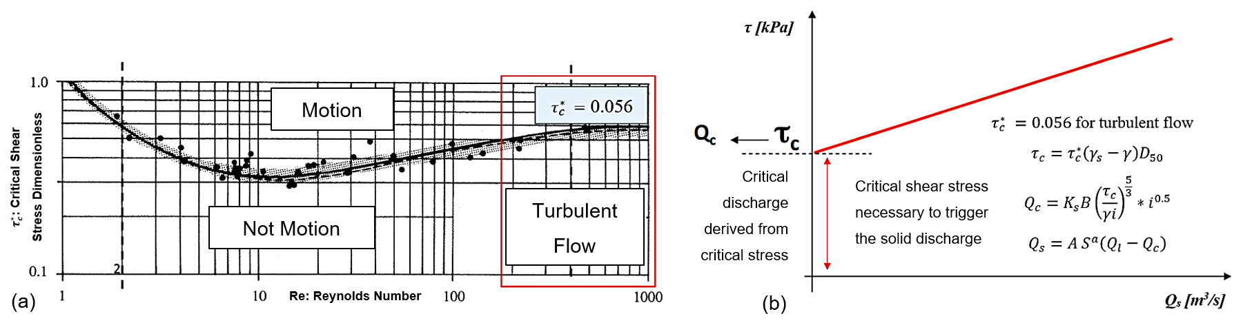
Figure 4(a) Shields (abacus) (Chow et al., 1988) for solid-transport incipient motion under different conditions of turbulence (Re: Reynolds number). In the red box the typical range of turbulent flow in rivers with a critical dimensionless shear stress of 0.056 is defined. (b) Evaluation of the incipient-motion condition for solid-transport discharge Qs using a power-law relation, where the critical shear stress τc [kPa] and the critical liquid discharge Qc [m3 s−1] are a function of saturated grain γs and γw and water-specific weights [kN m−3], the local granulometry through the parameter is D50 [mm], the roughness is KStrickler [–], the channel width is B [m], the reach slope is i [%], and the two coefficients are a [–] (between 1 and 2) and A [–] (between 0.94 and 5.8) (Vetsch et al., 2018).
The Gavrilovic method defines Ws as the source of available sediment routed through the watershed until the outlet. In CRHyME the sediment routing has been modelled considering its strong relation with the liquid discharge. First of all, the theory of incipient motion of Shields that states the starting motion of sediments in the function of the D50 quantity, the median diameter of the soil granulometric curve (Chow et al., 1988; Merritt et al., 2003; Vetsch et al., 2018), is implemented (Fig. 4). The solid discharge is evaluated in two ways. A first calculation considers a stream power formula for bed-load transport (Morgan and Nearing, 2011; Shobe et al., 2017; Campforts et al., 2020). Here, the solid discharge Qs [m3 s−1] is in the function of the channels's hydraulic and geometrical characteristics (Fig. 4), and it does not consider the local availability of the eroded material in the channel that may decrease/increase the amount of sediment delivered. This first implementation of solid-transport routing is also defined as transport limited (TL) since only the reached transport capacity is determined. A second calculation consists of an adaptation of the kinematic model for clear water to the sediment transport, under the hypothesis that the velocity of sediment transport is assumed to be similar to the water flow. The application of the kinematic method requires the estimation of stage–discharge relations for the sediment by analogy with the clear-water stage–discharge functions. Several authors (Govers, 1989; Govers et al., 1990; Rickenmann, 1999) have considered this hypothesis reasonable when no further additional information about solid transport is available. For this second case, the sediment balance is required, and it has been assessed in each cell domain through Eq. (16) considering the following: the erosion rate Es equal to the source term Ws computed by the EPM and the deposition rate Ds [m3 yr−1] and then divided by cell area and converted [m per time step] following Shobe et al. (2017); the transport term Ts considering the kinematic model adapted for sediment routing [m3 s−1] then converted [m per time step]; and the sediment amount hsolid(t) [m], converted to volume [m3] if multiplied by cell area extension [m2]. This second implementation is representative of the erosion-limited (EL) condition where the sediment availability in the river or across the slopes is limited by effective availability, as frequently happens (Shobe et al., 2017; Campforts et al., 2020; Chow et al., 1988; Davy and Lague, 2009).
In CRHyME both the TL and EL methods are evaluated for quantitatively assessing sediment transport yield within a physically reasonable range. According to Papini et al. (2017), Ivanov et al. (2020a), Dade and Friend (1998), Lamb and Venditti (2016), Peirce et al. (2019), Pearson et al. (2017), and Ancey (2020), the sediment transport dynamic is an active research frontier. In this sense, the spatial distribution of D50 is a critical point because it is difficult to be reconstructed at the catchment scale (Abeshu et al., 2022). Moreover, the D50 distribution influences the incipient-motion threshold that noticeably modifies the local sediment routing, leading to wrong estimations of the watershed sediment yield (Fig. 4). Since a close formulation does not exist for indirectly estimating the granulometry in the absence of an on-field survey dataset, empirical approaches have been proposed by Nino (2002), Sambrook Smith and Ferguson (1995), Lamb and Venditti (2016), and Berg (1995). According to these authors, morphological, climatic, hydrological and geological factors can influence river granulometry in a particular section. Slope-like factors have shown a quite significant correlation with D50, and in some cases slope → D50 relations (power laws in the form of were retrieved (Nino, 2002). Namely, D50 tends to increase with slope steepness. These relations mimic the formula proposed by Berg (1995), where D50 is indirectly determined using a power-law function describing the river morphology evolution. Even though slope → D50 represents a crude approximation, it has a physical meaning since in the upper catchment (where slopes are steepness) coarse granulometry is generally prevalent, while at the outlet (where slopes are lower) the sediment fine fraction becomes more significant (Tangi et al., 2019). In CRHyME, D50 is a necessary granulometric data point; therefore an ensemble of empirical slope → D50 curves have been proposed to automatically assess the D50 distribution across the catchment using the slope data. Curve parameters were calibrated ad hoc in the examined areas, comparing simulated sediment yields to the available measurements, and with on-site granulometry surveys.
Connections among simulated geo-hydrological processes
The processes described here may occur simultaneously inside a catchment, especially during heavy rains or after periods of prolonged precipitation (Abbate et al., 2021a). In CRHyME, the erosion and sediment transport are well integrated within the hydrological routines following the state of the art in the literature (Vetsch et al., 2018). Here, both the triggering function (sediment detachment and incipient motion) and the magnitude (amount of sediment eroded and transported) are quantified. On the other hand, for shallow landslides and debris flow, only the triggering condition of failure has been analysed, while the mass-wasting propagation across the catchment has not been included in the code yet. This choice is motivated by the fact that mass-wasting failures, especially for debris flows, are characterized by large uncertainties in their volume quantification related mainly to the entrainment processes, and their runout strongly depends on DEM accuracy and spatial resolution (i.e. spatial-scale dependency) (Jakob and Hungr, 2005; Scheidl and Rickenmann, 2011). The entrainment effect is difficult to be modelled in a closed form, and it may perturb the volume estimation by orders of magnitude (D'Agostino and Marchi, 2001). Mass-wasting processes may have a strong incidence on sediment transport dynamic, and compared to widespread erosion, which is a “low-intensity” process, landslides may abruptly change the geo-morphological characteristics of the catchment (Iida, 1999; D'Odorico and Fagherazzi, 2003). These issues are not investigated in this present work but are under study.
2.3 Model performance
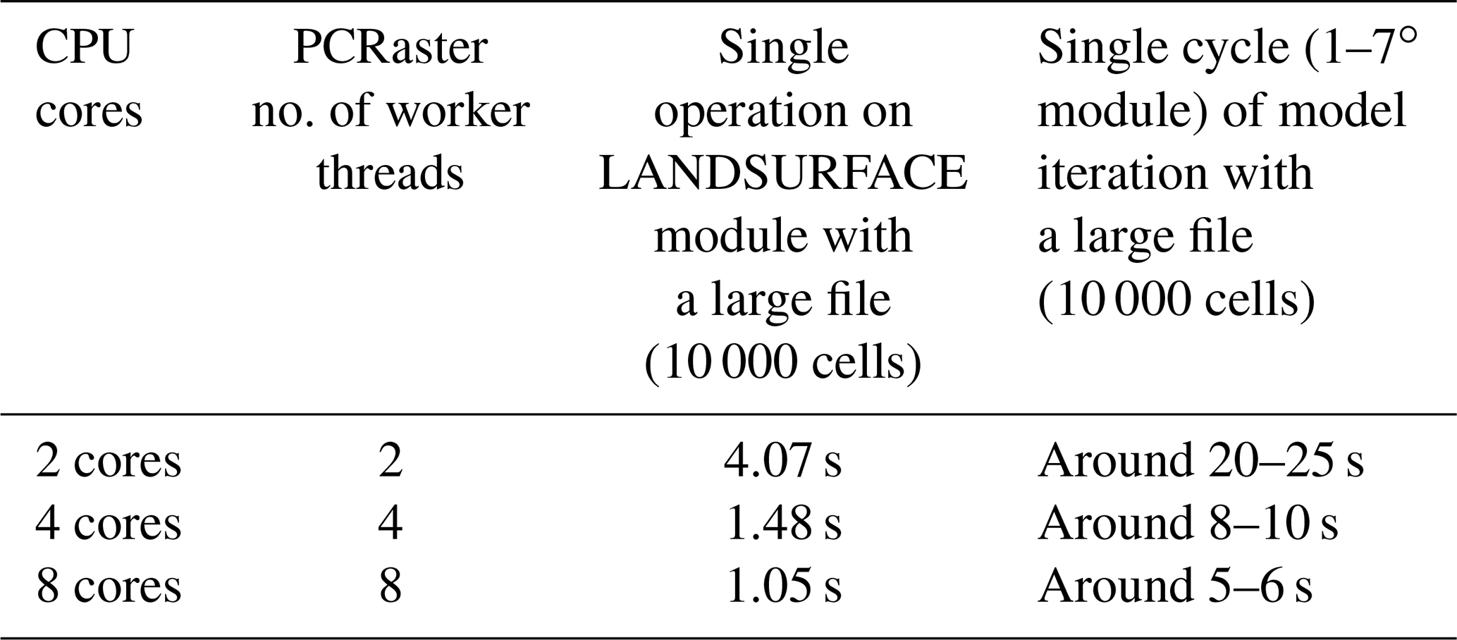
The PCRaster libraries implemented in CRHyME have the advantage of being fully parallelized to work with multicore processors (Karssenberg et al., 2010). This is an important aspect of our code that permits us to sharply decrease time-consuming work in each simulation. The intrinsic parallelization of the PCRaster libraries simplifies and facilitates code maintenance and updating, without any further optimizations. In Table 1 the operating-time calculation ranked for the CRHyME model is reported for different numbers of processor cores (worker threads).
Table 1Performance of the CRHyME model working on different CPU core sets. By increasing the number of cores available, the computation time for a particular operation can drop significantly.
2.3.1 Hydrological-error metrics and sediment transport assessment
Hydrological-performance assessment at basin outlets is evaluated through error indexes that compare water discharges recorded by the local hydrometer and the water discharge simulated by the model (Chow et al., 1988; Bancheri et al., 2020). The most common error metrics used in hydrology are the Nash–Sutcliffe efficiency (NSE) and the root mean square error (RMSE). The Nash–Sutcliffe efficiency (NSE) in Eq. (17) is a normalized model efficiency coefficient, where Si and Mi are the predicted (or simulated) and measured (or observed) values at a given time step i, respectively. The NSE varies from −∞ to 1, where 1 corresponds to the maximum agreement between predicted and observed values. The root mean square error (RMSE) in Eq. (18) is where Si and Mi are the predicted (or simulated) and measured (or observed) time series, respectively, and N is the number of components in the series.
For the sediment transport assessment, the periodical bathymetry campaigns carried out inside hydropower reservoirs can be considered a reference for the sediment yield measurement (Pacina et al., 2020; Langland, 2009; Marnezy, 2008). Compared to hydrometric data which can be easily gathered from local environmental agencies (Rete Monitoraggio ARPA Lombardia, 2023; Rete Monitoraggio ARPA Emilia-Romagna, 2023), bathymetries are generally not accessible to the public (ITCOLD, 2009, 2016). Therefore, the calibration and validation of erosion and sediment transport models have considered the seasonal volume estimation in hydropower reservoirs and the event-based volume estimation only where available. For the case studies analysed, these data were also retrieved from specific reports (Milanesi et al., 2015; Ballio et al., 2010; Brambilla et al., 2020).
2.3.2 ROC curves for local landslide prediction
According to Formetta et al. (2016), Pereira et al. (2016), Vakhshoori and Zare (2018), Gudiyangada Nachappa et al. (2019), Kadavi et al. (2018), and Fawcett (2006), a useful technique to assess the prediction performance of a slope stability model is the receiver operating characteristic (ROC) methodology. The ROC curve illustrates the diagnostic ability of a binary classifier system as its discrimination threshold is varied. In landslide stability assessment, the binary classification is the condition of FS ≥ 1 (stable) or FS < 1 (unstable) characterizing each pixel of the model domain (Formetta et al., 2016; Vakhshoori and Zare, 2018). In CRHyME, the number of landslide activations is counted. On each time step, a 0–1 map is produced where the destabilized pixels (FS < 1) are signed as 1, while stable pixels (FS ≥ 1) are signed with 0. This landslide-triggering algorithm is rather simple to implement inside a code, and other authors have also followed this approach (Harp et al., 2006; Milledge et al., 2014; Formetta et al., 2016). However, the inclusion of a pixel range in the surrendered area of a detected unstable pixel (prone to shallow-landslide failure) is necessary to describe the instability activation. Generally speaking, landslide instability areas are not confined to the landslide body but could extend to surrounding boundaries: in the upper part, the landslide crown could experiment with further collapse since other cracks may generate and propagate retrogressively (Ivanov et al., 2020b); in the bottom part, the landslide may evolve into soil slip or earth flow and travel along the slope following the maximum gradient (Jakob and Hungr, 2005); and the lateral boundaries could be also affected by landslide instability due to shear stress perturbation and reduced lateral roots cohesion (Rahardjo et al., 2014) that develops during landslide collapsing. Bearing in mind that a single-pixel slope failure evaluation may be not conservative from a hazard perspective, in CRHyME the unstable area related to the predicted unstable pixel has been extended also considering the surrounded eight adjacent cells, as reported in Fig. 6a.
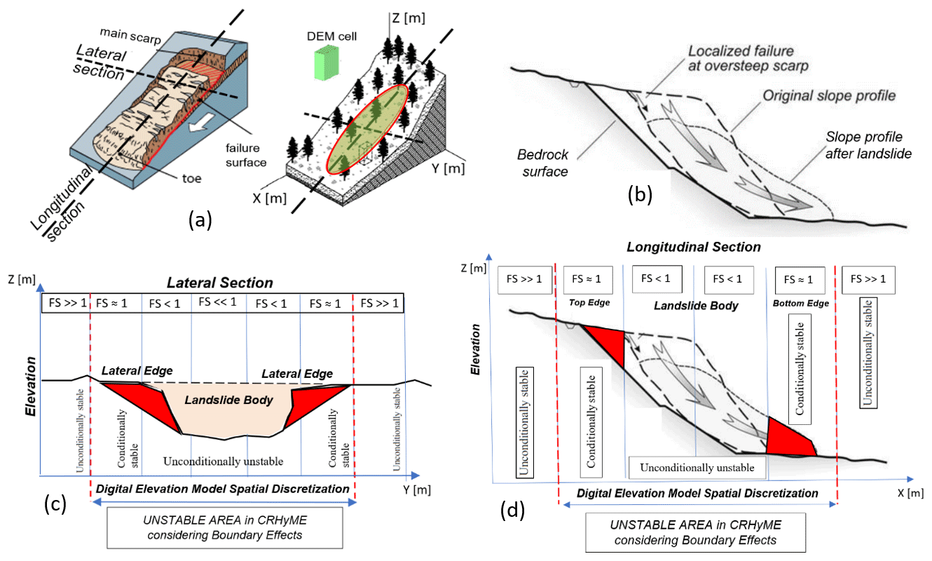
Figure 5Scale dependence in the infinite-slope stability assessment: (a) geometrical sections (longitudinal and lateral) of shallow landslides, (b) landslide kinematics along the longitudinal section, (c) exemplification of the stable and unstable areas in the lateral section, and (d) exemplification of the stable and unstable areas in the longitudinal section with respect to DEM resolution. In red the lateral, top and bottom edges of the landslide affected by instabilities are highlighted.
A nine-pixel counting may overestimate in some cases the extension of the hazardous area because it is also dependent on the DEM resolution. To assure the reasonability of this choice, a survey conducted within the IFFI (Inventario dei Fenomeni Franosi in Italia) landslide inventory (ISPRA, 2018; Guadagno et al., 2003; Guzzetti and Tonelli, 2004) has shown that typical rainfall-induced shallow landslides have mean and median spatial extension equal to ∼20 000 and ∼10 000 m2, respectively, which correspond to an indicative pixel size comprised between 150–100 m. In our case, the 90 m DEM resolution (sampled at the Equator) becomes ∼70 m at the latitude of the tested case study due to geographical transformation (Lehner et al., 2008). Therefore, a nine-pixel approximation could make the overall landslide extension equal to m2, slightly larger compared to the IFFI inventory range but within the same order of magnitude. However, the exact landslide geometry is not definable a priori since it has large variability in terms of extension and shape (areas mostly span 10 to 106 m2 according to Tanyaş et al., 2019), which could be larger or narrower compared to DEM resolution (Fig. 5a and c). Moreover, Oguz et al. (2022), Zheng et al. (2020), Legorreta Paulin et al. (2010) and Michel et al. (2014) have shown how the DEM resolution and its accuracy may significantly perturb the local stability at the top and bottom edges, extending or reducing the effective unstable slopes (Fig. 5b and d). According to Legorreta Paulin et al. (2010) a higher DEM resolution could improve the unstable area description by reducing size over-/underestimation, but it would noticeably increase the computational cost of the hydrological model (Zhang et al., 2016). These topics will be further discussed in Sect. 4.4.
Since the reference data on historical landslides in the IFFI inventory comes from several sources, the localization of the shallow instability could not be geo-localized with high precision, especially for historical events where sometimes only triggering-point locations (not the landslide polygon) are reported (ISPRA, 2018). To carry out the ROC methodology and avoid reference data issues, a buffer zone with different radii around each landslide point was created: 250, 500, 1000 and 2000 m (Fig. 6). This radius represents an attempt to cope with the uncertainties about the real position and extension of the triggered landslide.
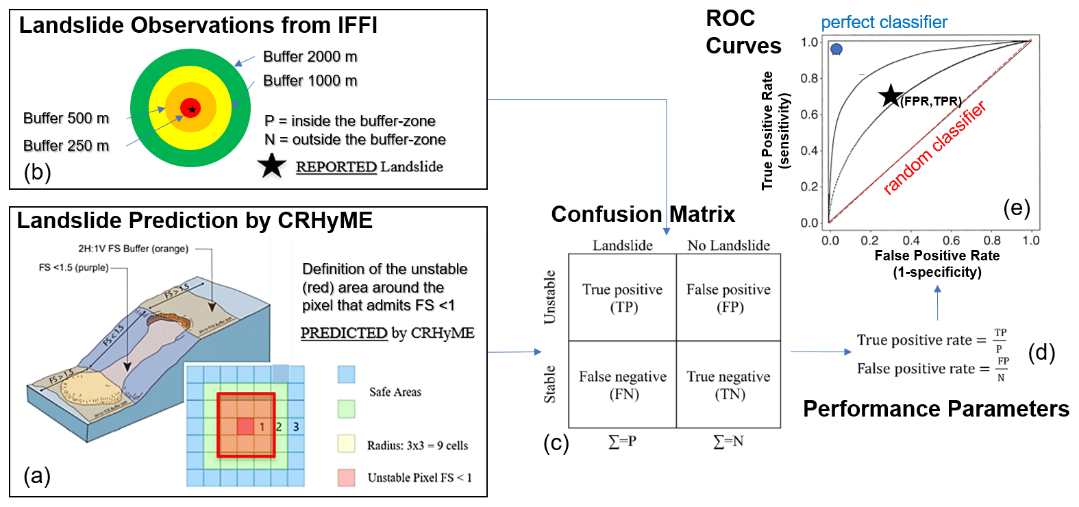
Figure 6ROC methodology scheme to assess the CRHyME model performance in detecting landslide failures that occurred after a rainfall event. (a) Unstable areas “predicted” by CRHyME considering the surrounding eight cells; (b) unstable area “reported” in the IFFI inventory considering buffer zones due to geo-localization uncertainties; (c) confusion matrix and calculation of parameters TP (true positive), FN (false negative), TN (true negative) and FP (false positive); (d) evaluation of performance parameters TPR (true-positive rate) and FPR (false-positive rate); and (e) graphical representation of the ROC curves.
Knowing the observed and the predicted instabilities (retrieved by the IFFI inventory and simulated by CRHyME) referring to a specific geo-hydrological event, the ROC assessment was conducted. The ROC curves were built following the scheme presented in Fig. 6. Through a confusion matrix (Fig. 6c), the false-positive rate (1 − specificity, FPR) (Eq. 19) and the true-positive rate (sensitivity, TPR) (Eq. 20) are calculated (Fig. 6d), and the point (FPR, TPR) is reported in the ROC graph (Fig. 6e). The upper left corner of the graph (TPR = 1 and FPR = 0) represents the perfect performance (or perfect classifier), and the diagonal line represents the random classification or no skill. As the point (FPR, TPR, the prediction skill) plotted on the ROC graph is closer to the upper left, the prediction capacity of the CRHyME model is better.
2.4 Cases studied
The case studies simulated with CRHyME are located in northern Italy and presented in Fig. 7.
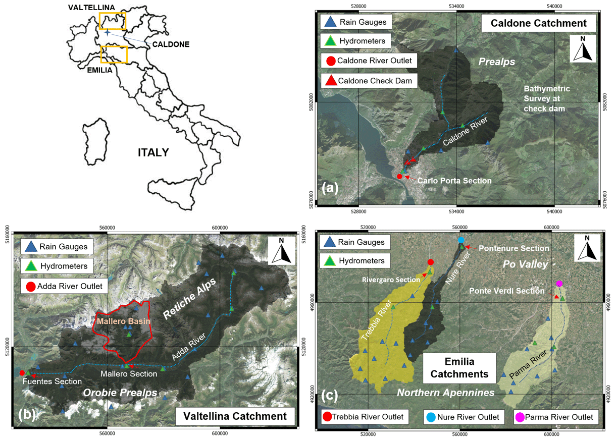
Figure 7The studied (a) Caldone, (b) Valtellina and (c) Emilia catchments. Rain gauges, hydrometer stations and river outlets are indicated in (a)–(c). Hydrometric stations considered for assessing the CRHyME performance are located at the sections of Carlo Porta (for Caldone River); Fuentes and Mallero (for the Adda and Mallero rivers) in the Valtellina catchment; and Rivergaro (for Trebbia River), Pontenure (for Nure River) and Ponte Verdi (for Parma River) across the Emilia area. Base layer from © Google Maps 2023. Retiche Alps: Rhaetian Alps, Orobie Prealps: Orobic Alps.
The Caldone basin (Fig. 7a) represents the on-field laboratory of the Politecnico di Milano (Brambilla et al., 2020). The basin is about 27 km2, is situated near the city of Lecco (region of Lombardy) across the Prealps and is characterized by intense sediment transport. The catchment is well monitored by five rain gauge stations; a hydrometer at the outlet; and two sediment check dams, where the sediment yield is constantly monitored with periodic bathymetric surveys. The lithology of the area is constituted by consolidated calcareous rocks with good strength properties but susceptible to rainfall erosivity. Karst is present in the surrounding region but is not relevant in the Caldone catchment (Papini et al., 2017). From a climatic viewpoint, the area has a mean precipitation of 2000 mm yr−1 (Rete Monitoraggio ARPA Lombardia, 2023).
The Valtellina catchment (Fig. 7b) is settled in the northern part of the region of Lombardy across the central Alps and in 1987 experienced a dramatic geo-hydrological episode triggered by intense and prolonged rainfalls (Abbate et al., 2021a). The effects on the territory were severe: shallow landslides, debris flows and flash floods were recorded, causing human injuries and fatalities and extensive damage to infrastructure and buildings (Luino, 2005). The secondary branch of Mallero River also experienced intense sediment transport during the 1987 flood, which affected the town of Sondrio. Similar events iteratively hit the area in November 2000 and 2002. The Valtellina Valley has E–W topographical development, and its geomorphology is characterized by a strong difference between the opposite slopes. In the southern flank of the valley, the Orobic Alps are constituted by consolidated metamorphic rocks (gneiss), while across the Rhaetian Alps (northern flank), magmatic and sedimentary rocks alternate with metamorphic ones. The most prevalent type of soil texture is formed by sandy loam and silty loam (Crosta and Frattini, 2003; Longoni et al., 2016). The catchment is characterized by a strong precipitation variability in the range of a minimum of 600 mm yr−1 in the north-eastern part of the Rhaetian Alps to a maximum of 3500 mm yr−1 in the south-western sector of the Orobic Alps (Rete Monitoraggio ARPA Lombardia, 2023). According to this, two different meteorological datasets were examined here to test the ability of CRHyME to deal with different rainfall datasets. The first one considers the meteorological data provided by the Regional Agencies for Environmental Protection (ARPA Lombardia) (Rete Monitoraggio ARPA Lombardia, 2023) ground-based weather stations. The second one is MERIDA, the MEteorological Reanalysis Italian DAtaset (Bonanno et al., 2019). MERIDA consists of a dynamical downscaling of the new European Centre for Medium-range Weather Forecasts (ECMWF) global reanalysis, ERA5, using the Weather Research and Forecasting (WRF) model, which is configured to describe the typical weather conditions of Italy.
The Emilia area is situated in the northern Apennines (Fig. 7c) and experienced intense geo-hydrological episodes in October 2014 and September 2015 (Ciccarese et al., 2020). Three watersheds were particularly affected: the Trebbia, Nure and Parma catchments. The event of October 2014 hit the Parma catchment, while the event of September 2015 hit the Trebbia and Nure catchments. From a geomorphological viewpoint, the northern Apennines represent a fold-and-thrust mountain chain where several landslide instabilities are present due to the post-failure weathering of claystone, sandstone and limestone rock fragments. These deposits are in residual strength conditions and can be quite easily mobilized and trigger debris flows during heavy rain episodes (Parenti et al., 2023). The region of Emilia is characterized by a rainfall distribution with a south–north gradient where a maximum amount of 2000 mm yr−1 is recorded in the highest relief of the Apennines (south), while the 700 mm yr−1 amount characterizes the floodplain areas of the Po Valley in the northern part (Rete Monitoraggio ARPA Emilia-Romagna, 2023).
During calibration and validation of the CRHyME model, some monitoring points for checking the water discharge and volume were chosen in correspondence with the reference hydrometers located at the catchment outlets (green triangles in Fig. 7a–c). Check dams and hydropower reservoirs were considered for estimating reference sediment yield: a check dam close to the outlet of the Caldone catchment (red triangles in Fig. 7a); three hydropower reservoirs of Campo Tartano, Valgrosina and Cancano for the Valtellina case study (red triangles in Fig. 10a); and AdBPo reference data (Autorità di Bacino Distrettuale del Fiume Po, 2022) for the Emilia case study. Regarding shallow landslides and debris flows triggered during the investigated geo-hydrological events, a literature survey has been conducted within the IFFI inventory and scientific literature to find an available inventory of the occurred failures (Figs. 11a and 13a).
In the next paragraphs, the results obtained for the three case studies are presented in the following way: describing the simulation settings, reporting the hydrological and sediment transport performance, and showing the landslide and debris flow ROC assessment.
3.1 Caldone case study
The Caldone catchment was investigated to verify the numerical conservativity of hydrological and sediment balances calculated by CRHyME to explore the sensitivity to the variation in spatial resolution of the input data (e.g. DEM) and to calibrate and validate the slope → D50 empirical relations. According to Rocha et al. (2020) and Tavares da Costa et al. (2019), a spatially distributed hydrological model is sensitive to input data spatial resolution. The reconstruction of the catchment parameters, such as the flow accumulation and the flow direction, depends on the characteristics of the DEM. As a result, routing methods, which also depend on the flow direction accuracy, may experience differences in results under different cell resolutions. Moreover, increasing the DEM resolution is time-consuming due to the considerable number of cells within the computational domain. To test these aspects in CRHyME, for the Caldone catchment four runs were executed in a short period of 6 months, considering four different DEM resolutions: 90, 50, 20 and 5 m. In Table 2 the simulation settings are resumed.
Table 2Settings adopted for the Caldone River simulations and the hydrological volume and discharge error metrics calculated at Carlo Porta hydrometric station, testing different DEM spatial resolutions.
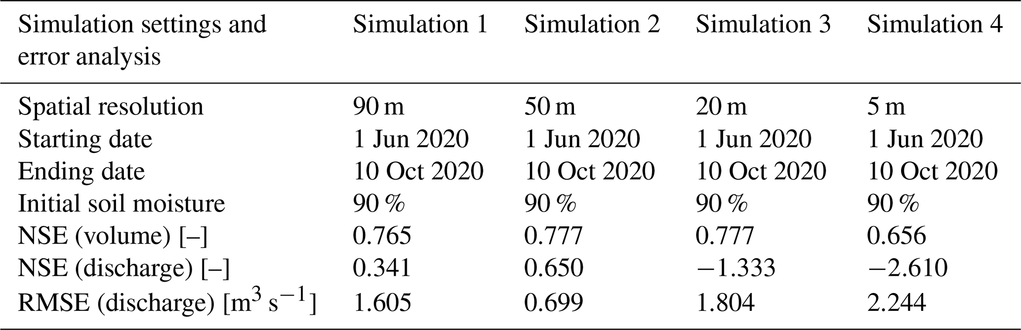
As can be seen in Table 2, the model's ability regarding the reproduction of a realistic water discharge tends to degrade progressively using a higher resolution. Looking at NSE scores for the discharge, the best accordance with the reference is reached with a 50 m resolution. The RMSE for the discharge is lower for a 50 m simulation. The model is conservative since the NSE for the volume is close to 0.8, verifying that almost all the precipitation volume has arrived at the outlet within the simulated period. The NSE for the volume is a parameter that is rather invariant with respect to the resolution, while the NSE for the discharge is dependent on the spatial scale. The meteorological data series necessary to run the model were gathered from ARPA Lombardia (Rete Monitoraggio ARPA Lombardia, 2023) (Fig. 7a). The hydrometer data and the local stage–discharge relation were retrieved from the station in the municipality of Lecco located at Via Carlo Porta (Fig. 7a). The rain gauges were spatially interpolated using the IDW technique (Chow et al., 1988) with a temporal resolution of 1 d.
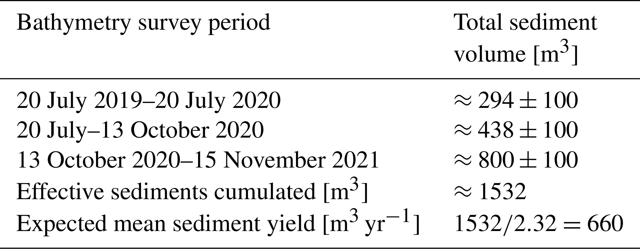
The influence of the slope → D50 curve parameterization was the second aspect investigated in the Caldone catchment. A long-term simulation has been carried out from 1 January 2019 up to 31 December 2021 (Fig. 8), with a DEM resolution of 50 m and after a spin-up period of 2 years for raising the model to realistic initial conditions. Considering the limited extension of the watershed, this period has been revealed to be sufficient for assessing the performance of solid discharge. The sediment discharge was computed considering both TL (transport-limited) and EL (erosion-limited) options. In Table 3 it can be seen that the NSE for water discharge and volume exhibit a high score, about 0.462 and 0.719, respectively. The former states that the reproduction of the hydrological part has been assessed almost correctly by CRHyME. Four slope → D50 functions have been tested in the form of (Table 4): set 1, set 2, set 3 and set 4. Results have shown that the choice of slope → D50 can noticeably modify the outlet's sediment yield: the cumulated sediment amount increases with a decrease in the mean diameter. These data were compared with the on-site bathymetric surveys that were carried out four times during the investigated period (Table 5). From the bathymetry measurements, a sediment yield of about 1000 m3 yr−1 was considered representative of Caldone River. In our sensitivity analysis, this value has matched the reference using set 2: 2993 m3 for 1055 d (≈3 years) corresponds to ≈1000 m3 yr−1. Set 2 is rather higher than the functions considered for Valtellina and Emilia simulations.
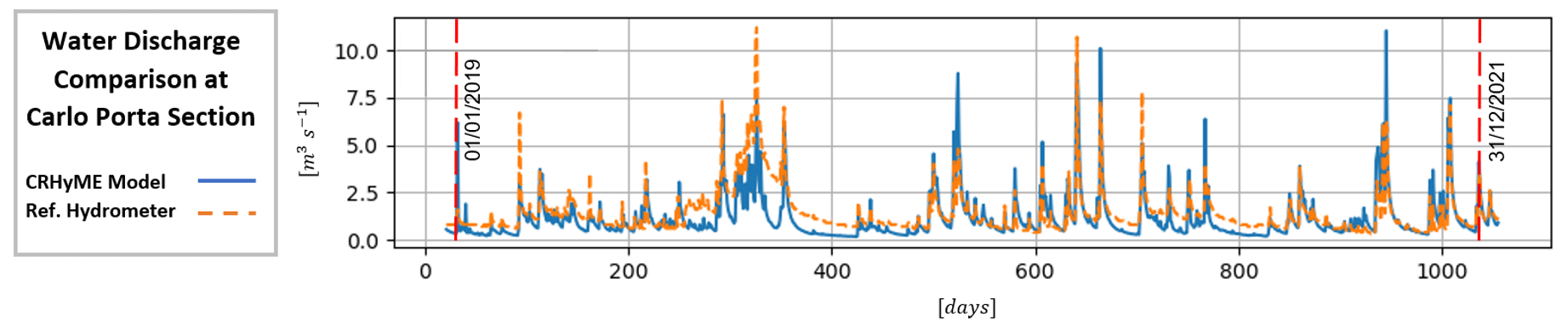
Figure 8Hydrological simulation carried out for sediment transport assessment in the Caldone catchment with 50 m DEM resolution from 1 January 2019 up to 31 December 2021: simulated water discharge (blue line) vs. reference hydrometer at the Carlo Porta section (orange line).
Table 3NSE and RMSE error metrics of the previous hydrological simulation for the volume and discharge quantities.
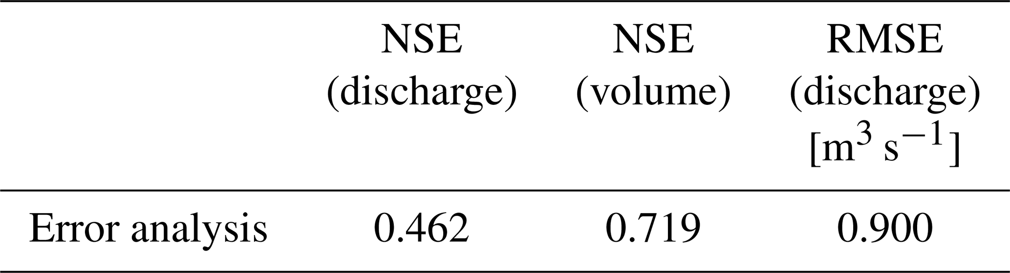
Table 4Slope → D50 functions tested in the Caldone catchment, and the volume of the total sediment simulated by CRHyME at the basin outlet.
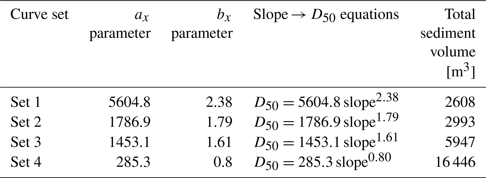
Table 5Bathymetric survey and total volume stored at the check dam close to the Caldone catchment outlet. An average sediment yield was calculated around 660 m3 yr−1. Due to possible measurement uncertainties and relatively short time series, a representative sediment yield value of 1000 m3 yr−1 was considered in the simulations.
3.2 Valtellina case study
The analysis conducted for the Valtellina area has followed the settings reported in Table 6. The CRHyME calibration was carried out for 3 years between 1 September 2015 and 31 August 2018 after a spin-up period of 2 years for acquiring realistic initial conditions. Then, a subsequent validation period started on 1 September 2018 and went up to 31 December 2019. In Fig. 9 the water discharges and the total volumes computed by CRHyME in the two reference sections of Fuentes (basin area of 2600 km2) and Mallero (basin area of 320 km2) are reported.
Table 6Simulation settings of the Valtellina case study. The calibration and validation of the model have considered using more than 4 years of data on a daily basis gathered from ARPA Lombardia (environmental agency) weather stations and the MERIDA reanalysis database (Bonanno et al., 2019). The calibration and validation of the model have considered more than 4 years of data on a daily basis gathered from ARPA Lombardia (environmental agency) weather stations and the MERIDA reanalysis database (Bonanno et al., 2019). These event-based simulations were carried out for significant geo-hydrological events of July 1987, November 2000, November 2002 and October 2018.
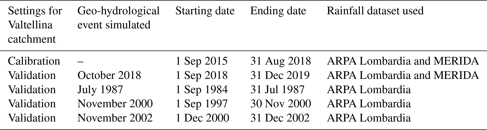
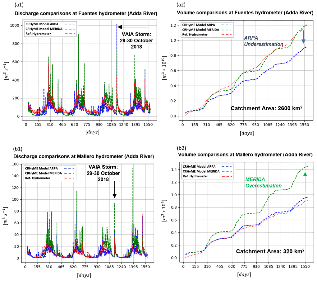
Figure 9CRHyME model simulation results of water (a1, b1) discharges and (a2, b2) volume at the (a) Fuentes and (b) Mallero hydrometers for the period 2015–2019 using ARPA weather stations and the MERIDA dataset. The geo-hydrological event that occurred in late October 2018 (Vaia storm; Davolio et al., 2020) has been recognized by CRHyME as one of the most intense, especially at the Fuentes section.
Looking at the simulation driven by the ARPA dataset, the total volume transited at the Fuentes section (blue line, Fig. 9a) is underestimated if compared to the local hydrometric reference (line red), while at the Mallero section (blue line, Fig. 9b) simulated and recorded volumes are in agreement. NSE scores for volumes also highlight this fact since Mallero's NSE is ∼1, while Fuentes's NSE is about 0.783 (Table 7). Transited volume is the integral of water discharge that has been better reproduced for the Mallero section (agreement among the blue and red line in Fig. 9b and NSE = 0.325 in Table 7) compared to that of the Fuentes section (disagreement among the blue and red line with underestimation of the mean flow during winter periods in Fig. 9b and NSE = 0.199 in Table 7) by the model.
Table 7NSE and RMSE error metrics of the previous hydrological simulation for the volume and discharge quantities. As can be appreciated, the volume performance is better than the discharge: the Valtellina basin is strongly regulated by hydropower plants and dams that operate a consistent lamination of the peak discharge lamination during major rainfall events; the kinematic routing may be not sufficiently accurate for flood propagation across the valley floodplain since dynamic lamination may occur. As a result, green and blue spikes overestimate the peak discharge compared to the reference.
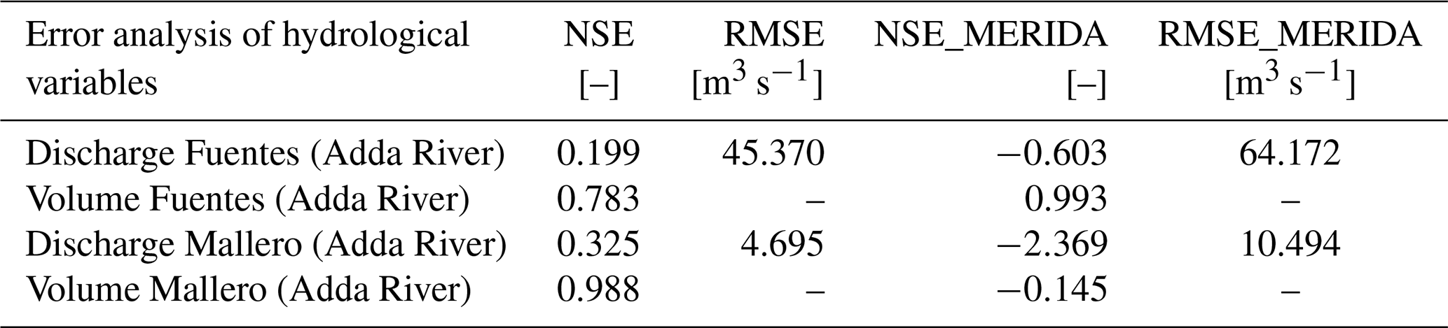
Opposite results were obtained considering MERIDA's dataset. There, the Fuentes section has performed well both in discharge and volume computation compared to the Mallero section. The volume NSE at Fuentes is now closer to the perfect agreement, while at the Mallero station the transited volume is noticeably overestimated. In both cases, NSE scores for discharges are badly represented with values below the 0 threshold. This fact is also well depicted in Fig. 9a and b, where discharge spikes simulated from the ARPA dataset (blue line) are lower compared to the green ones simulated from the MERIDA dataset. The CRHyME model performed numerically conservatively in both cases without code instabilities so that these outcomes are supposed to be perturbed by the different reconstructions of rainfall fields. From these results it can be noticed how the influence of rainfall data is determinant in the hydrological assessment. Looking at RMSE scores in Table 7, the simulation with the ARPA dataset was better performed, giving lower values of the index, around 4.7 and 45.4 m3 s−1 for the Mallero and Fuentes sections, respectively. This means that discharge uncertainties propagate proportionally, increasing the catchment extension, and CRHyME's performance is noticeably higher for small catchments.
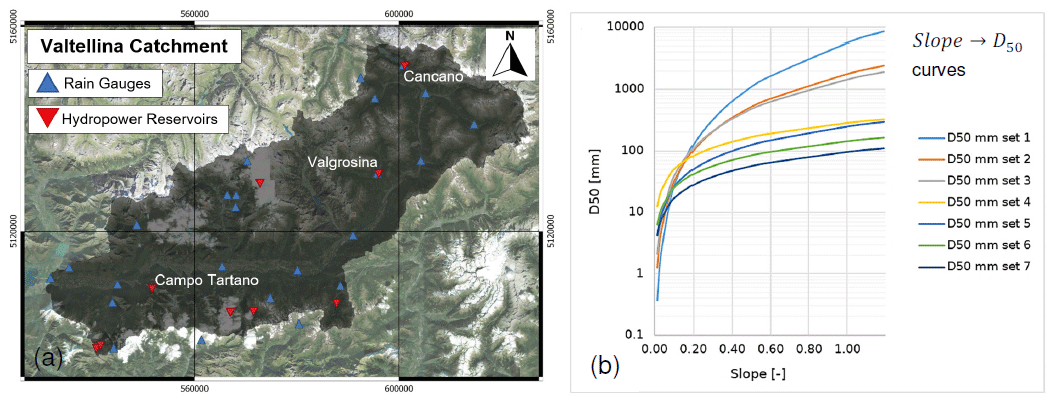
Figure 10(a) Valtellina case study area where hydropower reservoirs of Campo Tartano, Valgrosina and Cancano are indicated. (b) Slope → D50 relations tested and implemented in CRHyME based on the theory of Berg (1995) and Nino (2002) and considering on-site surveys. Base layer from © Google Maps 2023.
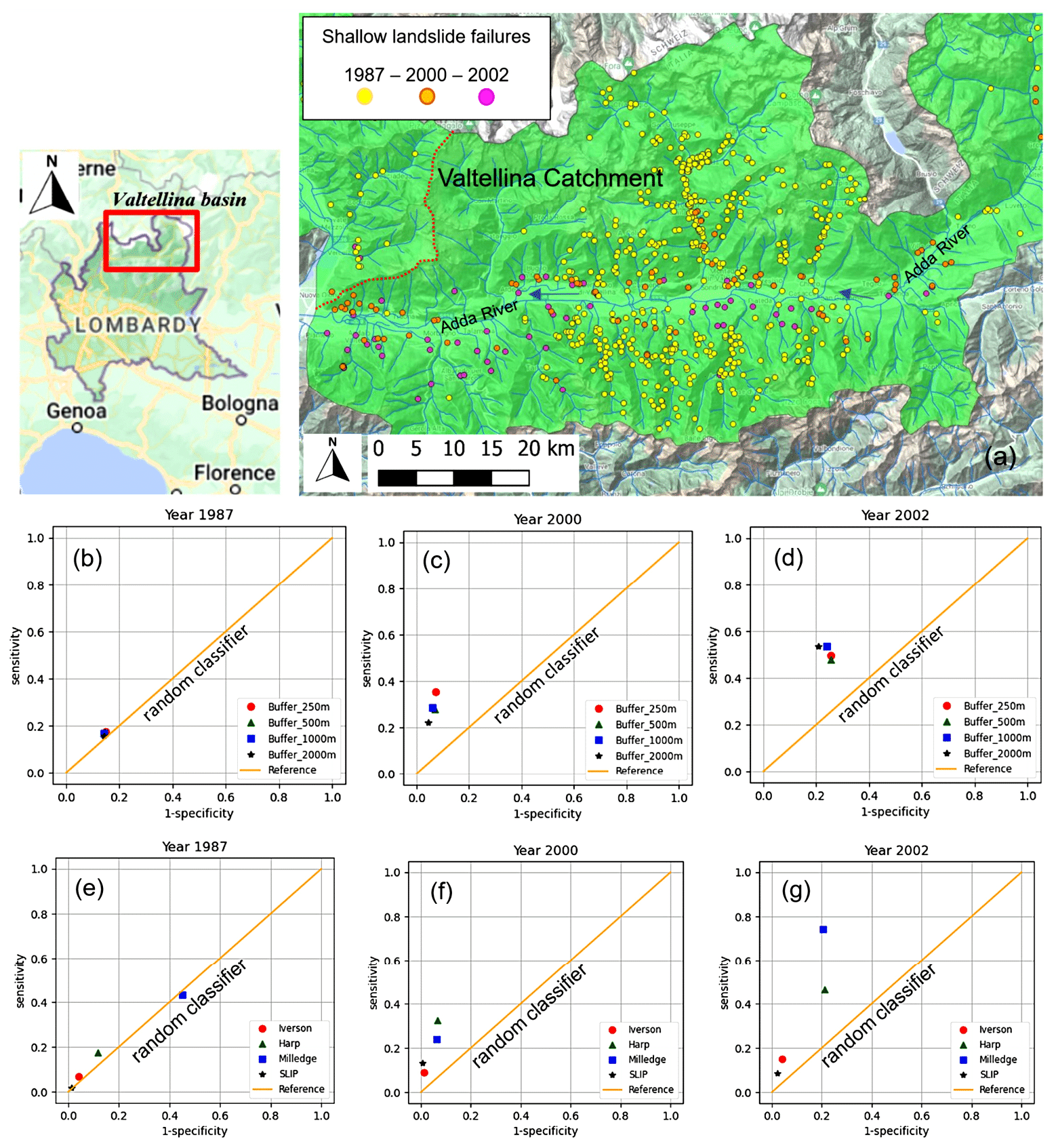
Figure 11(a) Triggered shallow landslides during the events of July 1987 (yellow points), November 2000 (orange points) and November 2002 (fuchsia points) reported by the IFFI inventory across the Valtellina area. (b–d) Representation of the ROC curves for the 1987, 2000 and 2002 events considering the Harp model with different landslide position's buffers of 250, 500, 1000 and 2000 m. (e–g) Representation of the ROC curves for the 1987, 2000 and 2002 events considering a buffer of 250 m and comparing the four stability models. The Milledge model behaved best for the 2002 event but was the worst for 1987, while the Harps model showed the most stable performance. Base layer from © Google Maps 2023.
Sediment transport results were checked in correspondence with the three hydropower reservoirs of Campo Tartano, Valgrosina and Cancano (Fig. 10a), considering ARPA dataset simulations. For each reservoir, a literature survey has been conducted to estimate the yearly mean sediment accumulation rate (Ballio et al., 2010; Milanesi et al., 2015; ITCOLD, 2016). The sensitivity parameter for sediment yield is represented by the slope → D50 curve that was adjusted during the calibration period (Fig. 10b and Table 8). Among others, set 6 was retained as it is sufficiently representative of the Valtellina area. In Table 9 the results obtained from CRHyME simulations show that the sediment yields evaluated yearly have matched the reference data for the three reservoirs investigated. For the Campo Tartano dam, the difference between the simulated and the reference is around −11.7 %, for the Valgrosina dam it is about +2.15 % and for the Cancano reservoir it is around −11.9 %.
Table 8Slope → D50 equations tested and implemented in CRHyME based on the theory of Berg (1995) and Nino (2002) and considering on-site surveys.
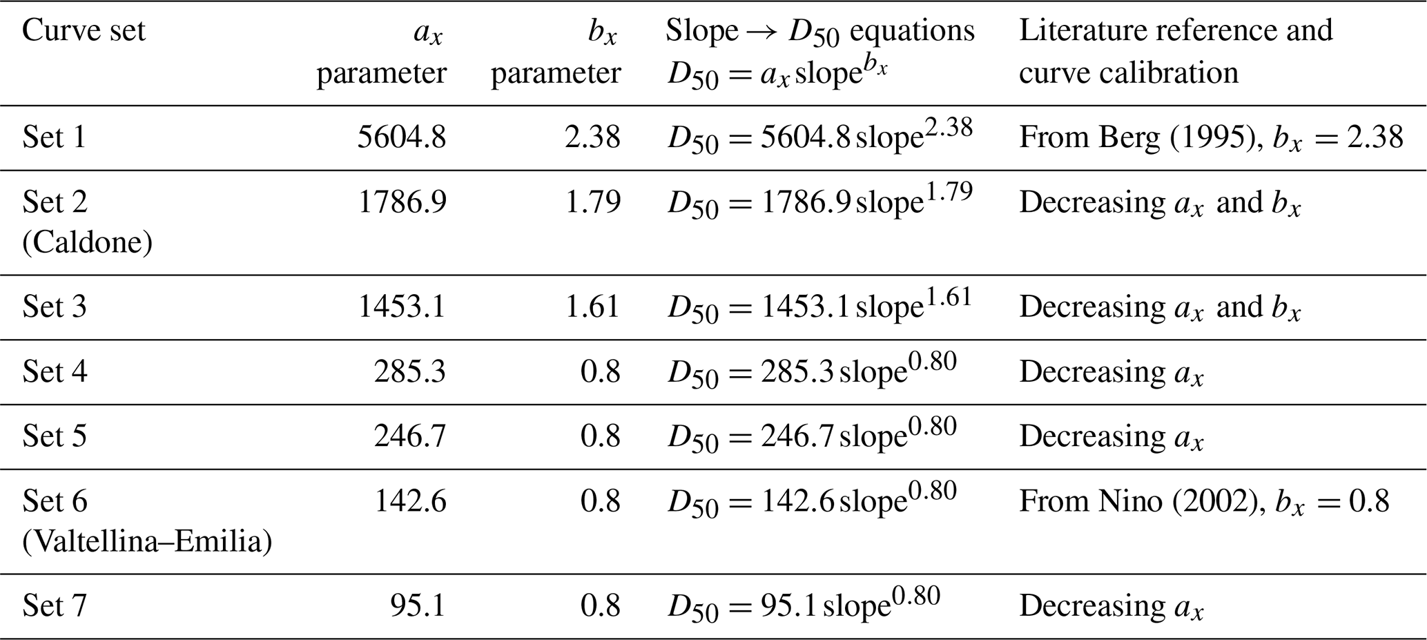
Table 9Sediment yields for the three dams of Campo Tartano, Valgrosina and Cancano, with the estimation compared to the ITCOLD reference (ITCOLD, 2009, 2016).
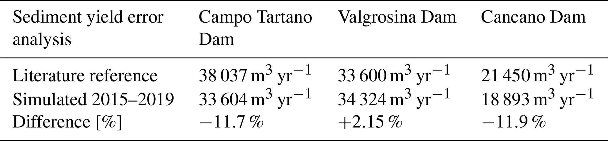
Table 10Simulation settings of the Emilia case study considering the ARPA Emilia-Romagna (environmental agency) rainfall and temperature data.
The capacity of CRHyME to predict the localization of shallow landslides triggered during the 1987, 2000 and 2002 events was investigated through the ROC scores. Figure 11b–d describes the ROC assessment for the shallow landslides that occurred across the Valtellina Valley during the July 1987, November 2000 and November 2002 events. The four shallow-landslide instability models included in CRHyME (Iverson, Harp, Milledge and SLIP) were compared, ranking the Harp model as the most accurate one (Fig. 11e–g) and with stable performance. A realistic combination of friction angle values was considered among the broader ranges available in the literature (Abbate and Mancusi, 2021a) – 40∘ for gravels, 35∘ for sand, 33∘ for silt and 30∘ for clay – similar to those proposed by Crosta and Frattini (2003). By analogy with root cohesion, the friction angle was spatially distributed by considering the soil composition (percentage of coarse material, sand, silt and clay as % coarse, % sand, % silt, % clay, respectively) within the superficial layers (Hengl et al., 2017). Using the Harp model for the three events, the ROC curves have assessed CRHyME's performance above the random-classifier threshold line. The sensitivity (true-positive rate) of the model is between 0.2 and 0.6, while the 1 − specificity (false-positive rate) is around 0.2. The distorted distribution of the shallow-landslide inventory related to 1987 may have influenced the performance predictions, lowering the ROC assessment compared to the events that happened in 2000 and 2002. The buffer's choice can influence the redistribution among TP and FP: the performance is slightly lower when large buffers are considered, especially for 1000 and 2000 m radii, while it tends to increase with the radius of 250 and 500 m close to the actual extension of the shallow landslide recorded.
3.3 Emilia case study
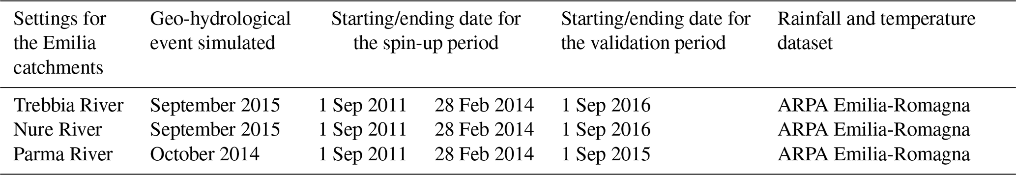
For the Emilia case study, CRHyME simulations were carried out considering 5 years from 1 September 2011 up to 1 September 2016, where the investigated geo-hydrological events of 13 October 2014 and 14 October 2015 have been recorded in the area (Table 10). To raise the model to a realistic initial condition, a spin-up period of 900 d comprised between 1 September 2011 and 28 February 2014 has been carried out. The ARPA Emilia-Romagna meteorological dataset (Rete Monitoraggio ARPA Emilia-Romagna, 2023) was considered for rainfall and temperature variables.
Table 11CRHyME model (a) error analysis for hydrological discharge and volume and (b) sediment yield for the Emilia catchments at the hydrometers of Rivergaro (Trebbia River), Pontenure (Nure River) and Ponte Verdi (Parma River).
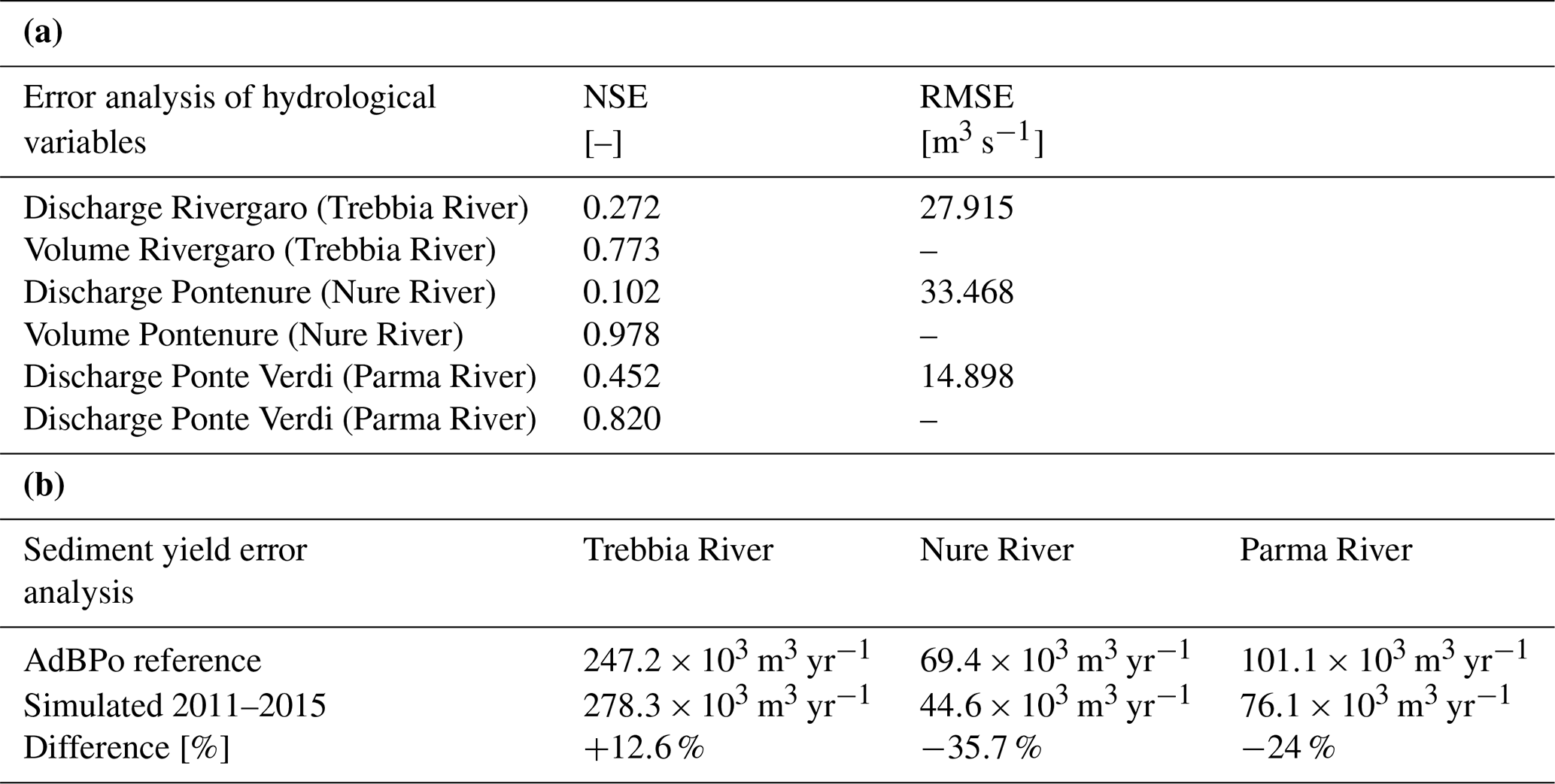
As seen in Table 11, the hydrology of the Trebbia, Nure and Parma rivers has scores similar to that of the Valtellina area (Fig. 12). Looking at the NSE in Table 11a, we can appreciate that higher scores are assessed for the water volume of the Nure (0.978), Parma (0.820) and Trebbia (0.773) rivers. For water discharges, NSE scores are better for the Trebbia (0.272) and Parma rivers (0.452), while for Nure River are lower (0.102), as is also confirmed by the RMSE index (Table 11a).
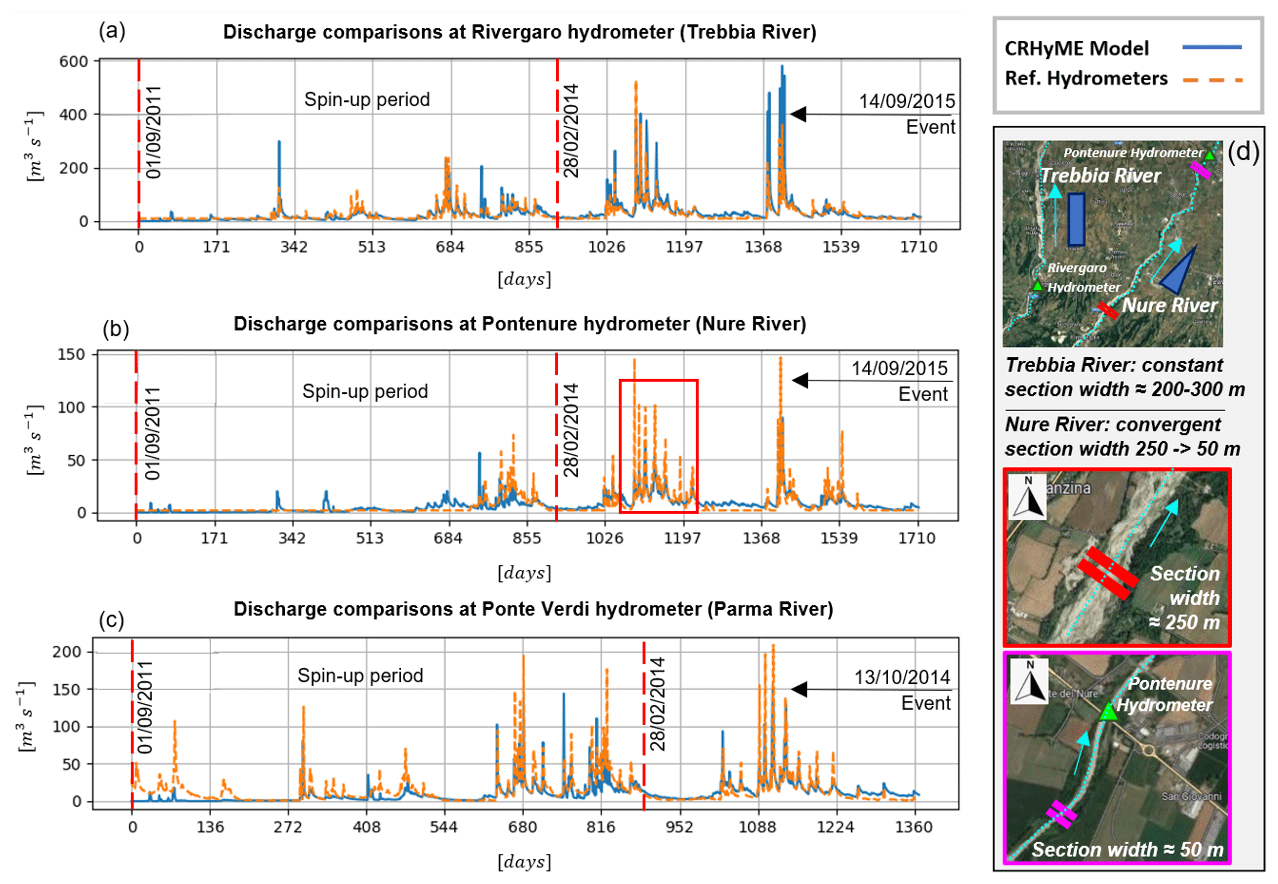
Figure 12CRHyME water discharges comparisons for the Emilia catchments at the hydrometers of (a) Rivergaro (Trebbia River), (b) Pontenure (Nure River) and (c) Ponte Verdi (Parma River) for the period 2011–2016. The first 900 d of each simulation is considered for model spin-up to a realistic initial condition. In the red box (b) the peak discharge underestimation for Nure River due to section variation along floodplain (d) is highlighted. Base layer from © Google Maps 2023.
Looking at the solid-transport quantification in Table 11b, the AdBPo (Autorità di Bacino del Fiume Po) reports were taken into consideration as reference data for the comparisons (Autorità di Bacino Distrettuale del Fiume Po, 2022). Keeping the same calibration of the slope → D50 curve (set 6) that was adopted for the Valtellina case (no granulometry data were found in the examined catchments), the results obtained after the simulations have shown fairly good accordance with the reference. In the three cases, the order of magnitude of the sediment yield delivered each year at the outlet is similar to AdBPo data, especially for the Trebbia (+12.6 %) and Parma (−24.7 %) basins, while for Nure we have a slightly larger difference (−35.7 %). Perhaps finer granulometry should have been taken into account for simulating the Parma and Nure rivers, decreasing D50. This suggests how the sediment transport dynamics are sensitive to the slope → D50 parameterization that strongly depends on the geological and lithological characteristics of the catchment.
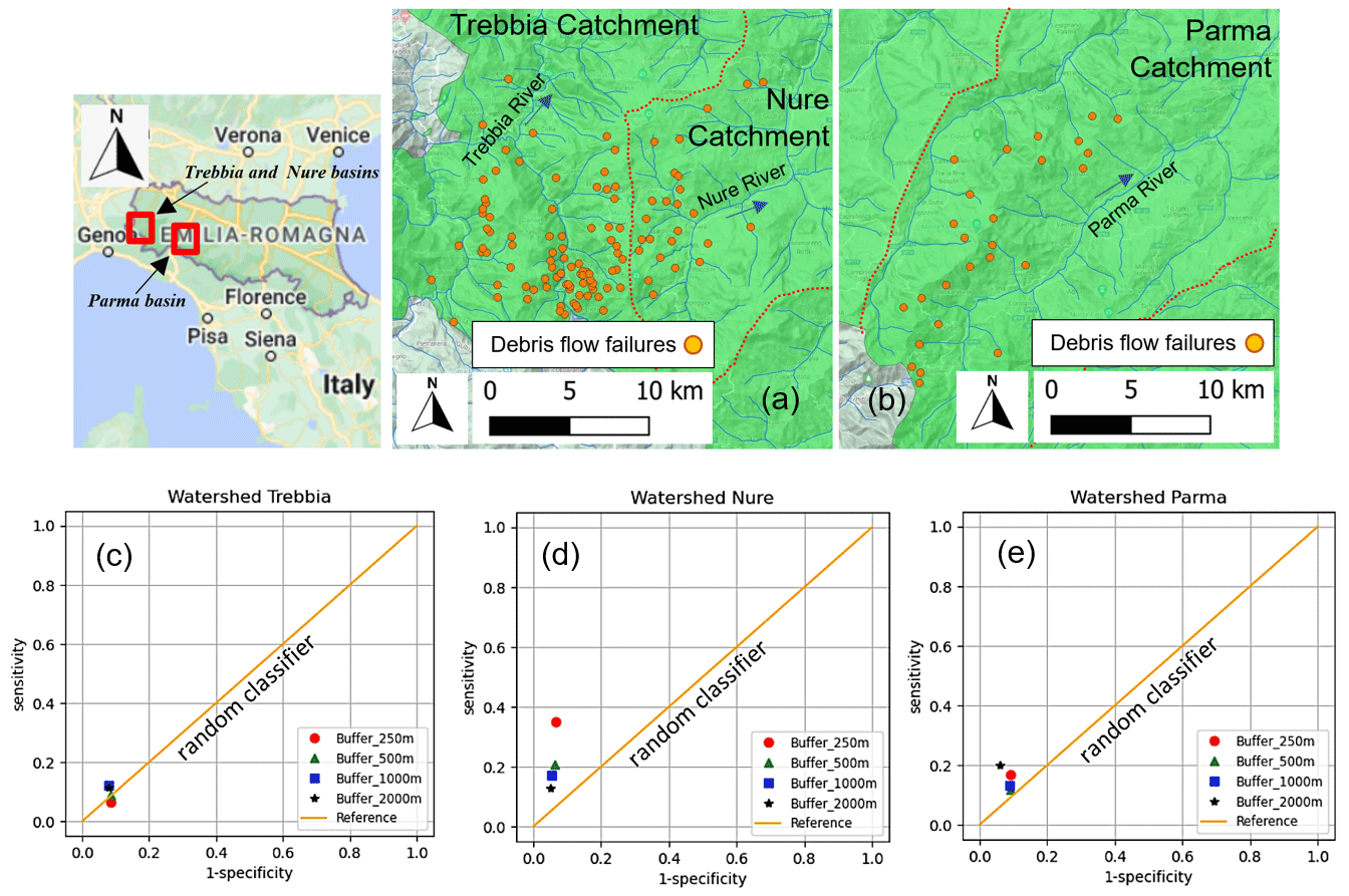
Figure 13(a) Debris flows triggered in the Trebbia and Nure basins during the event of September 2015 and (b) debris flows triggered in the Parma basin during the event of October 2014. Orange points are the mass-wasting starting points reported by Ciccarese et al. (2020, 2021) after the event. Representation of ROC curves for the Trebbia (c), Nure (d) and Parma (e) watersheds for the events of September 2015 and October 2014. Base layer from © Google Maps 2023.
The performance of CRHyME in detecting the triggered debris flow during the events of October 2014 and September 2015 (Fig. 13) was assessed again through ROC. A new calibration on the friction angle was carried out since the value provided for the Valtellina case was too conservative for stability. This fact could be explained by the Apennines's lithologies, which are characterized by higher percentages of clay compared to the central Alps, reducing the soil friction resistance (Raj, 1981; Hengl et al., 2017). The highest ROC scores were obtained by slightly decreasing (−20 %) the slope friction angles and reducing the soil cohesion to the minimum, which is supposed to be representative of incoherent deposits. In most cases the model has outperformed the random classifier, showing a sensitivity (TPR) comprised between 0.1–0.4 and a higher value of specificity (1 − FPR) depending on the chosen buffer extension around the triggering point. In our simulations, debris flow failure has been effectively detected across a small valley impluvium, confirming the on-site observations carried out by Ciccarese et al. (2020, 2021): the highest scores were obtained for the Nure catchment, with an intermediate rank for the Parma basin and a poor description of instabilities for the Trebbia watershed.
4.1 CRHyME sensitivity analysis: spatial resolution and sediment diameters
The CRHyME model sensitivity in reproducing hydrological cycle has been tested considering four different spatial resolutions within the Caldone catchment (27 km2): 90, 50, 20 and 5 m. CRHyME results were obtained with sufficient accuracy and a faster computation for cell resolution of > 10 m. The computational time was observed to be proportional to the number of domain cells: the 90, 50 and 20 m simulations were concluded in 1 to 2 min, while for the 5 m simulation, the time was raised to 5 min. However, increasing spatial resolution does not mean always increasing the accuracy (Rocha et al., 2020; Zhang et al., 2016), and with CRHyME the best performance was acquired for DEM resolutions of 50 m and 20 m and not for 5 m. The variation in the DEM resolution can noticeably change the flow direction of the rivers (ldd.map) and the basin drainage density, affecting discharge computation. According to the literature (López Vicente et al., 2014; Erskine et al., 2006), the routed runoff could be perturbed by numerical diffusion, a known problem of the spatially distributed models that is predominant with fine spatial resolution, which depends on the algorithm applied for flow direction computation (Barnes, 2016, 2017). To preserve CRHyME's solution accuracy and to maintain affordable computational times, we suggest applying the HydroSHEDS DEM model at 90 m resolution for quite large basins of > 500 km2, while higher resolutions are advisable for smaller basins.
Within the Caldone catchment, the dependence of the sediment transport processes on the soil granulometry was tested. The distribution of D50 that increases as a function of the slope is a reasonable representation of the geomorphological processes encountered in mountain catchments (Brambilla et al., 2020; Ivanov et al., 2020a; Ballio et al., 2010). According to Nino (2002), there is a slight correlation between slope and D50, but non-linearities are caused by sediment processes occurring within river granulometry (sorting and armouring). Recently, data-driven approaches were explored in the USA to define a map of D50 along the river stream (Abeshu et al., 2022). To evaluate the map, these authors have chosen a series of geo-morphological predictors of D50 (elevation, slope, curvature, etc.); verifying results with the available databases at country-based levels, they have retrieved the USA D50 map. Not surprisingly, one of the most important predictors is the basin slope which has the highest correlation coefficient with D50, but other geomorphological factors (river path length and elevation) have a similar correlation with D50. It seems clear that a unique formulation of D50 as a function of morphological and hydrodynamical parameters cannot be assessed straightforwardly. Since D50 is required for incipient motion of bed-load sediment transport (Chow et al., 1988) and bearing in mind its complexity in spatial evaluation, slope → D50 curves implemented in CRHyME represent a crude but efficacious simplification. Moreover, slope → D50 curves have the advantage of being easily calibrated if on-site data are available.
4.2 CRHyME's hydrological performance
For the Valtellina case study, CRHyME hydrological performance for the water discharge (NSE ∼ 0.2–0.3) was not comparable to that obtained for Caldone River (NSE ∼ 0.46). A possible explanation resides within the characteristics of the Valtellina catchment, which is bigger (2600 km2) than the Caldone basin (27 km2). Bigger computation domains mean increased landscape heterogeneity, which implies higher uncertainties in the reproduction of infiltration–runoff–groundwater processes (Morbidelli et al., 2018; Mishra et al., 2003; Chow et al., 1988). Comparing volume and discharge scores for the Valtellina area driven by the ARPA dataset, a general tendency to overestimate the peak discharge during rainfall seasons (spring, summer and autumn) can be noticed, while an underestimation of the discharges during winter is detected (Fig. 9a). This effect is more significant at the Fuentes hydrometer but is less evident at the Mallero station. After analysing these results, three main error components were disentangled into (1) infiltration, (2) losses and (3) routing parameterizations. They represent key processes that should be paid attention to during the calibration phase (Morbidelli et al., 2018), since if they are wrongly conditioned, they may also cause numerical instabilities, losing the water balance conservativity of the code. As reported by Abbate and Mancusi (2021a), infiltration models strongly regulate runoff generation. Their parameterization depends on land surface coverage and terrain composition, which are sometimes affected by high uncertainties: on-site measurements are generally not available, and coverage layers have low resolution. For CRHyME, this fact may imply cascade effects on landslide processes causing underestimation of the landslides triggered due to the reduced subsurface pore pressure caused by wrong soil moisture balance predictions. Water recirculation inside the groundwater reservoir affects water balance in the long term. In this regard, the Alps and Apennines have complex hydrogeology (ISPRA, 2018), which affects the groundwater dynamics that a simple Dupuit model may oversimplify. Unfortunately, the unavailability of local piezometric reference data for calibration has not permitted us to assess model performance for this part. To cope with these uncertainties, several sensitivity and calibration tests (not reported here) were conducted during model construction, varying the groundwater parameterization to achieve the best performance. Another source of error is embedded in the runoff-routing algorithm. The kinematic algorithm adopted in CRHyME is sufficiently representative of the small lateral catchment rainfall-runoff processes (as for the Caldone or Mallero rivers) but may not be suitable for interpreting floodplain flood evolution where dynamic processes are prevalent (Chow et al., 1988). Moreover, across the Valtellina catchment, river discharges are regulated by several hydropower plants (ITCOLD, 2009, 2016). Dams can smooth and shift floods peaks and perturb seasonal water discharges recorded at the outlet's hydrometer, lowering the CRHyME performance: in the current version of the model, lakes and dams are not considered explicitly. Among other things, this fact could explain the best water discharge score (NSE = 0.325) of the Mallero subcatchment (less regulated, only two dams) with respect to the Fuentes outlet (NSE = 0.199) for the whole Valtellina catchment (Fig. 7).
The hydrological performance of the Emilia catchments has scores similar to Mallero River. The water discharge assessment for the tested period shows the best agreement for Trebbia (NSE ∼ 0.27) and Parma (NSE ∼ 0.45). These basins are less regulated by hydropower reservoirs compared to the Valtellina case, and, since they are smaller (about one-third of the extension), the kinematic approach for runoff routing is more representative. Nevertheless, the lower scores for Nure River were caused by an underestimation of the peak discharges (Fig. 12). Several simulations conducted in the Nure basin have shown a systematic bias within the reference data. The latter could be explained by the location of the reference hydrometer, which is settled far away across the flood plain where the river is constricted to flow within a narrow section (∼10 m) compared to the upper catchment (∼250 m) (Fig. 12d). Looking at Fig. 7, the Pontenure (Nure River) hydrometer is located across the flood plain, ∼ 20 km downstream of the catchment for the Rivergaro (Trebbia River, ∼1 km) and the Ponte Verdi (Parma River, ∼10 km) stations. Similarly to the Valtellina case, where a flood lamination is likely to occur, to describe river behaviour across a floodplain, the dynamic approach should be preferred instead of kinematic routing. In fact, including section geometry as input could increase the simulation accuracy, improving the model's performance in hydrographs and discharge reconstruction (Lee and Pin Chun, 2012; Chow et al., 1988).
4.3 CRHyME's geo-hydrological performance
Geo-hydrological processes have been consistently reproduced by CRHyME. The sediment yields in the Valtellina catchment have matched the available reference data of the Campo Tartano, Valgrosina and Cancano dams after a calibration of slope → D50 to distribute grain size parameters across the catchment. The good reproduction of the annual sediment yield (∼10 % underestimation for the Valtellina case) has been confirmed also for the Emilia case study, where the order of magnitude was comparable to the AdBPo reference ( % depending on the basin).
Since D50 perturbs the threshold that activates the sediment transport (Vetsch et al., 2018), it has revealed the critical parameter to be assessed in the CRHyME model. For the Valtellina and Emilia areas, the optimal slope → D50 curve (set 6, Fig. 10) was different compared to the one adopted for the Caldone catchment (set 2, Fig. 10). From a geological viewpoint, the Caldone catchment is located in the Prealps, where calcareous rocks are prevalent, while metamorphic bedrock is more diffused across the Valtellina catchment (ISPRA, 2018). Depending on the state of fracture, metamorphic bedrock could be less strong than calcareous rocks and more prone to being fragmented into small diameters (D'Agostino and Marchi, 2001). Moreover, the maturity of the watershed influences the granulometry distribution across the landscape (Pérez-Peña et al., 2009; Strahler, 1952). Large basins such as the Valtellina and Emilia catchments are more mature than the small Caldone catchment; therefore, a finer granulometry at the outlet is expected. This fact seems to justify why a lower slope → D50 curve was optimal for these catchments, while a higher one was more suitable for the Caldone basin.
The CRHyME model has identified the localization and the timing of landslide failures during the extreme events that have affected the studied catchment. Looking at ROC scores for the Valtellina area, the 1987, 2000 and 2002 events were reproduced consistently. The best scores were acquired for 2000 and 2002 events, where a good quality inventory was available for the investigated area. For 1987, the incompleteness of the available inventory (yellow points in Fig. 11a) affected the model's final score. However, independently from the specific case, the ROC methodology has highlighted how much the choice of the stability parameters (friction angle and cohesion) has a critical influence on the final results. This fact has also been confirmed by the sensitivity analysis carried out for debris flow episodes in the Emilia case study during the events of 2014 and 2015. Here, to reach the best ROC scores against the random classifier, the friction angles calibrated for the Valtellina case have been slightly reduced by about 20 %, confirming the dependence of this parameter on soil texture and lithology.
4.4 Model limitations
The sensibility of the CRHyME model to precipitation mapping, initial hydrological conditions, DEM scale dependency and the geo-hydrological cycle parameterization have affected the result accuracy and performance. Since they represent possible limitations on the applicability of the code, a brief discussion is developed here, suggesting possible solutions.
Correctly assessing the precipitation distribution is mandatory to define a realistic representation of the external forcing that triggers geo-hydrological failures (Abbate et al., 2021b). Especially across mountain regions, the higher local variability in meteorology and the absence of a dense rain gauge network can complicate the reconstruction of a representative rainfall field. This aspect was investigated for the Valtellina case study, where simulations derived by the MERIDA (Bonanno et al., 2019) and ARPA (Rete Monitoraggio ARPA Lombardia, 2023) datasets were compared. Using MERIDA, we would expect a better performance from CRHyME, but this did not happen in all situations. Looking at water volumes transited across the Fuentes hydrometer during the period 2015–2019, the MERIDA dataset has performed better than ARPA stations. On the other hand, looking at the Mallero hydrometer, the MERIDA dataset has scored worse than ARPA stations. What is the possible explanation for this contradictory fact? MERIDA gives a rainfall map that has a spatial resolution of ∼4 km, while the ARPA station data are interpolated geometrically using the inverse distance weight (IDW) techniques (Daly et al., 1997; Chow et al., 1988). A trade-off exists between the ARPA's rain gauge network density and the spatial resolution of MERIDA. In large catchments, MERIDA is more representative since it can cover ungauged areas, while, in small catchments, lower spatial resolution may be insufficient for describing local rainfall variability. This is why MERIDA has performed worse than IDW in the Mallero catchment, where several ground-based weather stations are uniformly distributed across a limited area of 320 km2 (Fig. 7). Moreover, reanalysis datasets could sometimes smooth the rainfall peaks, leading to a wrong interpretation of the net rainfall that occurred over a limited area (Abbate et al., 2021b; Bonanno et al., 2019; Ly et al., 2013). This is another key issue that generally influences the ability of the slope stability model implemented in CRHyME to detect landslides triggered by rainfalls. In this regard, a better integration within rainfall sources coming from the ground-based station, reanalysis models, radar maps and satellite data are advisable to reduce possible rainfall uncertainties (Abbate et al., 2021b).
The choice of a realistic initial catchment's moisturizing is another common issue in every deterministic spatially distributed hydrological model (Uber et al., 2018; Tramblay et al., 2010; Chow et al., 1988). Historical measures about the superficial soil moisture, groundwater piezometry and superficial runoff are difficult to gather, especially across small mountain basins where monitoring systems are not provided (Schoener and Stone, 2020; Chiarelli et al., 2023). Moreover, soil moisture is a quantity that can vary abruptly across different terrain types, so it is not common to implement a network that permits the acquisition of distributed information across a catchment (Lazzari et al., 2018). In CRHyME, to overcome these difficulties, a spin-up period was introduced within each simulation. This period represents the minimum time required by the model for reaching an automatic adjustment of the initial condition that, depending on the extension of the basin, can be comprised from within a few months up to a few years. The spin-up simulation permits a re-distribution of the water across the cells of the domain (horizontally) and among each layer of the model (vertically), reducing the time lag between rapid (runoff) and slow (groundwater) catchment dynamics. This time lag effect was rather evident for the Emilia case study, where a realistic regime condition was reached only after 3 years, which is slower than for the Adda basin (2 years). This fact could be explained by the different soil compositions and lithology that influence hydrogeological parameters. In the Apennines, the presence of clay decreases the speed of soil recharge (lower permeability), slowing down the groundwater recharge (Ronchetti et al., 2009; Ciccarese et al., 2020; Parenti et al., 2023) compared to the Alps, where coarser terrain granulometry increases soil permeabilities. From a practical viewpoint, running the model up to realistic hydrological conditions is time-consuming. In CRHyME, PCRaster libraries are already parallelized and can noticeably reduce the computational cost of this operation. Moreover, CRHyME can set a restart condition, saving the hydrological storage outputs hsnow(t), hsoilwater(t), hgroundwater(t) and hrunoff(t) computed during the spin-up period which could be reused for subsequent running.
For evaluating shallow-landslide and debris flow triggering the simple theory of the infinite-slope stability model has been implemented. According to Harp et al. (2006), Iverson (2000), Takahashi (2009), Oguz et al. (2022) and Milledge et al. (2014), this methodology is rather affordable for cell-based landslide susceptibility models and mapping thanks to its fast coding. However, different results in the slope stability assessment are expected to vary depending on DEM resolution. This fact was not directly experienced with CRHyME since in the Caldone catchment, where spatial-scale dependence was tested, the IFFI inventory was not available for landslide investigation. Legorreta Paulin et al. (2010) and Zheng et al. (2020) have pointed out how the simple infinite-slope theory needs to be applied carefully. First of all the inaccuracy of the infinite-slope method is related to the fact that each pixel is considered independent of the others settled at the boundary (Iverson, 2000). For a very large DEM pixel size, namely >100 m, this may be an acceptable hypothesis since 100×100 m2 represents the typical order of magnitude of a rainfall-induced shallow landslide or a debris spatial extension (∼10 000 m2). For pixels ≤ 100 m this is not properly correct since the cell size is lower than the typical dimension: surrounding areas may participate in the landslide collapse due to boundary effects, especially at the top and bottom edges (Fig. 5), caused by strength redistribution (Zheng et al., 2020; Milledge et al., 2014). In CRHyME, with a spatial resolution of about ∼70 m, we have preferred to include the surrounding eight pixels close to the unstable areas, following a rather conservative choice justified by the physical interpretation of landslide kinematics. On the other hand, a varying DEM resolution causes a modification of the local slope gradients which are the main drivers of failure: lower resolutions can operate an unphysical smoothing of the surface, reducing the cliff and scarp that may trigger small landslides. As a result, the best DEM resolution available may lead to the most accurate results, but this choice is generally adopted for static landslide susceptibility mapping, but it may not be suitable for dynamic routines (Legorreta Paulin et al., 2010; Zhang et al., 2016). In CRHyME hydrological balance is computed at each time step, and then the slope stability calculation is evaluated recursively: increasing the spatial resolution, the computational times rise fast so that a trade-off between model performance and result accuracy should be acquired. Bearing this in mind, improvements on landslide hazards are planned in the future version of the code, making the slope stability routine less scale-dependent and less conservative.
According to Gariano and Guzzetti (2016), reconstructing the whole geo-hydrological cycle that drives the erosion and mass-wasting processes through numerical models is a challenge. In this regard, CRHyME is not an exception: the EPM is considered for erosion; empirical power-law relationships are implemented for sediment routing; and only conditions for landslide and debris flow triggering are evaluated by stability models, not including runout evolutions. This subdivision was adopted firstly to simplify the phenomenon interactions and secondly to guarantee the fast functioning and stability of the CRHyME code. Following this sequential scheme, geo-hydrological processes are computed after the hydrological assessment, but possible feedbacks are not explicitly taken into account. On a long-term timescale, geo-hydrological processes contribute to a landscape modification, e.g. DEM height changes. The former is not included by CRHyME since the code has been built with a different purpose with respect to landscape-evolutions models (Campforts et al., 2020; Bovy et al., 2020; Salles, 2019). However, all geo-hydrological hazards also play an important role in the short-term period, temporarily or permanently modifying the local soil depth (Sklar et al., 2017): landslide and debris flow runout can redistribute the local terrain, changing the soil depth (asportation at the crown and accumulation at the toe) and modifying the DEM height. Therefore, finding a closure for the superficial geo-hydrological balance is a non-trivial task from a theoretical and numerical viewpoint (D'Odorico and Fagherazzi, 2003). The CRHyME experience has shown how landslides and debris flow stability assessment cannot be treated deterministically since their triggering strongly depends on the choice of the model type (FS equations) and on stability parameters (the friction angle and the cohesion), which are parameters generally measured in the field or in a laboratory. In CRHyME, following some literature studies (Hengl et al., 2017; Yu et al., 2018; Chow et al., 1988; Dade and Friend, 1998), the cohesion was spatially distributed in the function of vegetation coverage, bearing in mind that roots contribute to stability, while the friction angle was correlated with the soil composition. On the other hand, the friction angle is a function of the soil texture, granulometry and consolidation, also depending on complex sediment dynamics and geological processes (de Vente and Poesen, 2005; Merritt et al., 2003; Shobe et al., 2017; Ballio et al., 2010; Kondolf, 1997). As a result, the calibration procedure within a sensitivity analysis was necessary on a case-by-case basis since these parameters correlate with several geo-morphological predictors.
The assessment of the superficial geo-hydrological cycle cannot be evaluated precisely since its monitoring is currently still insufficient on a catchment scale (ISPRA, 2018; Gariano and Guzzetti, 2016). Even though surface mapping and inventory are supposed to increase their accuracy and completeness in the future thanks to remote sensing data (Ciampalini et al., 2016), some doubts remain about the possible improvements for other fundamental data required for slope stability and sediment transport routines. However, the databases adopted in CRHyME (Hengl et al., 2017; Huscroft et al., 2018; Ross et al., 2018) represent the very first attempt to overcome these issues, having already made an important homogenization of the essential data required for geo-hydrological modelling.
Geo-hydrogeological processes have been conventionally studied separately in many engineering fields (hydrology, geology, etc.). Hypotheses and simplifications adopted to make them more tractable have sometimes partially neglected their mutual interactions, possible chain effects and embedded interdisciplinarity. Therefore, hydrological models that jointly assess the erosion and sediment transport processes and evaluate shallow-landslide instabilities are quite rare. In this sense, the CRHyME model was designed as a tool able to show a complete picture of the most significant geo-hydrological processes that may occur at the catchment scale.
CRHyME model was built ex novo using the Python programming language, implementing faster PCRaster libraries that can simulate hydrological processes in a very efficient way. CRHyME includes some of the common features of the classical, spatially distributed hydrological model, but its focus is on quantitative reconstruction of geo-hydrological hazards. CRHyME is characterized by six modules that reproduce hydrological balance over terrain and by a brand-new module deputed to simulate erosion, solid transport, and shallow-landslide and debris flow triggering at the catchment scale. In the field of geo-hydrological risk assessment, the integration of all those processes in a spatially distributed hydrological model represents a novelty.
Since the aim of our study was to build and facilitate the usage of the model indistinctly in any area of the globe, a deep investigation of the open-source repositories available for initial data has been carried out. The user-defined calibration parameters have been reduced to the minimum. Among them, erosion coefficients, average sediment diameters, cohesion and friction angle have been tuned following the strategies presented above. A sensitivity analysis has been carried out to simplify and accelerate the reconstruction of realistic hydrological initial conditions, adding the possibility of activating the restart option after a spin-up period. Moreover, the DEM's resolution-scale dependency was investigated and detected by the results.
CRHyME was intensively tested to make it as general as possible and reproducible in whatever catchments. Our case studies, the Caldone basin, the Valtellina catchment and the Emilia area, were chosen looking at the availability of historical data which are of paramount importance for model validation. The results have shown a fairly good reproduction of the past observations: the model is numerically stable (thanks to PCRaster libraries), conservative (no water or solid leakages outside the domain) and hydrologically consistent (compared to the reference hydrometers, the routed water volume shows an NSE ≈ 0.8–0.9, while discharges have lower performance, NSE ≈ 0.2–0.4, especially for larger catchments regulated by hydropower plants); the solid discharge reproduced with a downscaled EPM using Gavrilovic's method is consistent with the observations (errors around ±20 %), even though there are some uncertainties in the D50 parameter; and the triggering of shallow landslides and debris flows is comparable in number and spatial localization to the reference inventory (confirmed by ROC assessment). However, CRHyME's performance is rather sensitive to the quality of rainfall field data that should be accurate in spatial and temporal resolution to allow the code to correctly detect landslide triggering.
The efforts conducted with the creation of CRHyME go in the direction of a better investigation of geo-hydrological hazards. CRHyME is a multi-hazard model able to address and quantify at the catchment scale several geo-hydrological processes that may occur simultaneously, are physically coupled and cannot be interpreted separately. With CRHyME it is possible to overcome the software fragmentation in the geo-hydrological field, answering the recent need of multi-hazard quantification required not only in back analysis studies but also for a multi-risk nowcasting at the civil-protection level.
In this section, an example of the CRHyME .INI file is reported. Each module contains the parameters, variables and other settings required for the computations. The .INI file reports the simulation time settings (e.g. starting date and ending date), the spatially distributed input data and the meteorological and climatological data series, the options of each computational module, and the name of the output files. The .INI file is read by the deterministic_runner.py file that starts the CRHyME model and its internal routines (Fig. 2): in preprocessing.py, reporting.py and plot.py modules, variables are defined, saved and plotted, respectively, following the formats and standards of the PCRaster libraries (Sutanudjaja et al., 2018; Karssenberg et al., 2010). CRHyME's results are reported in two formats, a .csv data sheet or a .netcdf map (Jacob et al., 2014; Sutanudjaja et al., 2018). The first type is used to pick up information about a particular quantity at one location such as in correspondence with a rain gauge or hydrometric station. The data sheet is organized with a first column containing the time step value, while the subsequent columns contain information picked from one or more monitoring points. The .netcdf maps are produced to store information about the states and fluxes variables of the model. At each time step, the quantity at the spatial resolution of the DEM model is saved within the .netcdf stack. The variable required to be sampled should be specified in the .INI file under reporting options: for .csv files a .map file containing the location of sample points, while for .netcdf the name of the variable required should be specified. Using the GDAL libraries for Python (GDAL/OGR contributors, 2020), the input–output geographical data have been converted to the PCRaster standard format .map for raster data (Karssenberg et al., 2010; Sutanudjaja et al., 2018), considering the WGS84 datum as a reference system for geographical projection. The following are found in the output's files: the lateral water fluxes Fsub(t), FGW(t) and Fkin-dyn(t) [m3 s−1]; the vertical water fluxes CI(t), Sml(t), I(t), ETc(t), R(t), Lper(t), Ex(t) and ExGW(t) [mm per time step]; and storage quantities hsnow(t), hsoilwater(t), hgroundwater(t) and hrunoff(t), which are converted into cubic metres simply by multiplying the storage height (from [mm] to [m]) by the cell area extension of the DEM [m2]. Further description of the submodules can be found in the CRHyME's manual (Abbate and Mancusi, 2021a, b).
| .INI FILE EXAMPLE | |
| [globalOptions] | (CRHYME'S GENERAL OPTIONS) |
| inputDir = ModelCRHyME\CRHyME_Inputs_Trebbia | (input directory) |
| outputDir = ModelCRHyME\CRHyME_Outputs_R | (output directory) |
| cloneMap = map\clone.map | (clone map for delimiting domain) |
| institution = RSE_Ricerca Sistema Energetico | (institution name) |
| title = CRHyME project | (project title) |
| description = by Andrea Abbate and Leonardo Mancusi, resolution = 90 m | (project description) |
| resolution = 90 | (spatial data resolution) |
| startSeries = 31 Dec 1985 | (starting data of series)1 |
| startTime = 1 Jan 1986 | (starting data of simulation)1 |
| endTime = 30 Dec 2005 | (ending data of simulation)1 |
| timestep = 24 | (time step resolution in hours) |
| stampTimestep = 1 | (stamp time step in no. of time steps) |
| Restart = 1 | (activate restart option after spin-up) |
| Restart_Snow = \restarts\mod2\Restart_Snow.map | (snow height state for restart) |
| Restart_Surface = \restarts\mod2\Restart_Surface.map | (runoff height state for restart) |
| Restart_Soil = \restarts\mod2\Restart_Soil.map | (soil water height state for restart) |
| Restart_Ground = \restarts\mod2\Restart_Ground.map | (groundwater height state for restart) |
| Restart_SoilSed = \restarts\mod2\Restart_SoilSed.map | (sediment height state for restart) |
| [climaOptions] | (CLIMA MODULE OPTIONS) |
| CLIMA_Switch = 1 | (enable reanalysis climatic input data) |
| Rain_NC4 = netcdf\eucordhi_mod2_pr_day.nc | (.netcf reanalysis climatic input data) |
| [meteoOptions] | (METEO MODULE OPTIONS) |
| input_tab = tab | (folder containing .tab (txt) data sheet) |
| mask = map\mask01.map | (0–1 mask map, equal to clone.map) |
| DEM = map\DEM_clip.map | (elevation model DEM.map [m]) |
| z0 = tss\mod2\Z0_eucordhi_mod2_tas_day.tss | (regression temp–elev: intercept) |
| TempRatio = tss\mod2\TCoef_eucordhi_mod2_tas_day.tss | (regression temp–elev: angular coeff) |
| z0MAX = tss\mod2\Z0_eucordhi_mod2_tasmax_day.tss | (intercept for max temp) |
| TempRatioMAX = tss\mod2\TCoef_eucordhi_mod2_tasmax_day.tss | (angular coeff for max temp) |
| z0MIN = tss\mod2\Z0_eucordhi_mod2_tasmin_day.tss | (intercept for min temp) |
| TempRatioMIN = tss\mod2\TCoef_eucordhi_mod2_tasmin_day.tss | (angular coeff for min temp) |
| infilRain_file = tss\2011_2016\Rain_TREBBIA_Precipitazione_ALL.tss | (rain gauge time series .tss (txt))2 |
| mayrainstat = map\Rain_Stations_Trebbia.map | (rain gauge location .map)2 |
| LAT = 43 | (latitude) |
| ETC_Switch = 1 | (evapotranspiration calc enabled) |
| Aspect = map\Aspect_Filled.map | (aspect file .map [–]) |
| Slope = map\Slope_Filled.map | (slope file .map [–]) |
| mysoilmap = map\CLC_9Cat.map | (use of soil .map) |
| Kc_FAO = tbl\Kc_FAO.tbl | (Kc coefficient for FAO evapotrans)3 |
| Albedo = tbl\Albedo.tbl | (albedo coefficient for FAO evapotrans)3 |
| [interceptionOptions] | (SNOW AND INTERCEPTION MODULE |
| OPTIONS) | |
| input_tab = tab | (folder containing .tab (txt) data sheet) |
| LAImax = tbl\LAImax.tbl | (LAI maximum index)4 |
| LAImin = tbl\LAImin.tbl | (LAI minimum index)4 |
| SNOW_Switch = 1 | (snow calc enabled) |
| [landSurfaceOptions] | (LAND SURFACE MODULE OPTIONS) |
| input_tab = tab | (folder containing .tab (txt) data sheet) |
| INF_Switch = 2 | (infiltration calc enabled)5 |
| sand_sup = map\Sand_SUP90C.map | (% sand on surface soil at 10 cm depth) |
| silt_sup = map\Silt_SUP90C.map | (% silt on surface soil at 10 cm depth) |
| clay_sup = map\Clay_SUP90C.map | (% clay on surface soil at 10 cm depth) |
| CoarseFrc_SUP = map\CoarsFrg_SUP90C.map | (% coarse on surface soil at 10 cm depth) |
| myrivermap = map\PathRiverSM.map | (river location .map)6 |
| Loss_River = tbl\Loss_RIV.tbl | (reduction coeff for river losses)6 |
| Inf_CLC = tbl\Infiltr_CLC.tbl | (infiltration coeff (soil use)) |
| CN_I = map\CN_I.map | (SCS-CN method CN I .map) |
| CN_II = map\CN_II.map | (SCS-CN method CN II .map) |
| CN_III = map\CN_III.map | (SCS-CN method CN III .map) |
| Initial_SM = 0.9 | (initial condition of soil moisture) |
| SoilDepth = map\BDRICM_M.map | (soil depth .map [cm]) |
| MaxWatStgTOP = map\TSH1_clip.map | (% max water storage soil at 10 cm depth) |
| MaxWatStgBTM = map\TSH5_clip.map | (% max water storage soil at 1 m depth) |
| sand_btm = map\Sand_BTM90C.map | (% sand on surface soil at 1 m depth) |
| silt_btm = map\Silt_BTM90C.map | (% silt on surface soil at 1 m depth) |
| clay_btm = map\Clay_BTM90C.map | (% clay on surface soil at 1 m depth) |
| CoarseFrc_BTM = map\CoarsFrg_BTM90C.map | (% coarse on surface soil at 1 m depth) |
| [groundwaterOptions] | (GROUNDWATER MODULE OPTIONS) |
| input_tab = tab | (folder containing .tab (txt) data sheet) |
| Sr_Falda = 0.8 | (initial condition of groundwater table) |
| Idro_Map = map\Idrogeology_Emilia_Trebbia.map | (hydrogeological .map)7 |
| Ks_GLHYMPS_exp = map\GLHYMPS_Emilia_Trebbia.map | (saturated permeability from GLHYMPS)7 |
| Permeability = tbl\IdrogeologyTabs\Permeability.tbl | (saturated permeability .tbl (txt))7 |
| Anisotrophy = tbl\IdrogeologyTabs\Anisotrophy.tbl | (anisotropy coefficient .tbl (txt))7 |
| Porosity = tbl\IdrogeologyTabs\Porosity.tbl | (porosity coefficient .tbl (txt))7 |
| Storativity = tbl\IdrogeologyTabs\Storativity.tbl | (storativity coefficient .tbl (txt))7 |
| Type_Depth = tbl\IdrogeologyTabs\Type.tbl | (hydrogeological reclassify .tbl (txt))7 |
| [landSlidesOptions] | (LANDSLIDE MODULE OPTIONS) |
| LANDSLIDE_Switch_1 = 2 | (landslide trigger calc enabled)8 |
| C_Veg = tbl\C_Veg.tbl | (cohesion from vegetation .tbl (txt)) |
| Surcharge = tbl\Sur_Veg.tbl | (cohesion from vegetation .tbl (txt)) |
| X_Gavrilovic = tbl\X_Gavrilovic.tbl | EPM X (soil protection) coefficient .tbl (txt)9 |
| Y_Gavrilovic = tbl\Y_Gavrilovic.tbl | EPM Y (soil erodibility) coefficient .tbl (txt)9 |
| LithoY_Gavrilovic = map\Idrogeology_Emilia_Trebbia.map | EPM Y (soil erodibility) lithology .map (map)9 |
| FI_Gavrilovic = map\Kst_Emilia_Trebbia.map | EPM FI (type of erosion) coefficient .map (map)9 |
| [routingOptions] | (ROUTING MODULE OPTIONS) |
| ROUTING_Switch = 1 | (enable calc routing) |
| lddMap = map\ldd_clip.map | (ldd .map of flow directions) |
| cellAreaMap = map\cellsizeArea.map | (map of cell area extension) |
| River_Pit = map\Pit_Point.map | (basin outlet location) |
| Strickler = tbl\Ks_Strickler.tbl | (Strickler–Manning coefficient) |
| SectionTable = tbl\Dynamic\Sections2.tbl | (section (type table .map)10 |
| [reportingOptions] | (REPORTING MODULE OPTIONS) |
| mysamples_real = map\Idro_Samples_Trebbia.map | (real-hydrometer sampling .map) |
| mysamples_fake = map\Idro_Samples_F.map | (other-hydrometer sampling .map) |
| mysamples_solid = map\Solid_Samples.map | (reservoir sampling .map) |
| outDailyTotNC = CumFails,CumFails_D | (daily counted .netcdf)11 |
| outMonthTotNC = P,Etc | (monthly counted .netcdf) |
| outMonthAvgNC = T | (monthly averaged .netcdf) |
| outMonthEndNC = CumFails,CumFails_D | (end-monthly counting .netcdf)11 |
| outAnnualTotNC = P,Etc | (annual cumulated .netcdf) |
| outAnnualAvgNC = T | (monthly averaged .netcdf) |
| outAnnuaEndNC = CumFails,CumFails_D | (end-annual cumulated .netcdf)11 |
| formatNetCDF = NETCDF4 | (.netcdf specified format) |
| zlib = True | (enable .netcdf creation) |
Table A1Description of the .INI file modules implemented in the CRHyME model. GLHYMPS: GLobal HYdrogeology MaPS, EPM: erosion potential method, CLC: CORINE Land Cover, FAO: Food and Agriculture Organization, SCS-CN: Soil Conservation Service curve number.
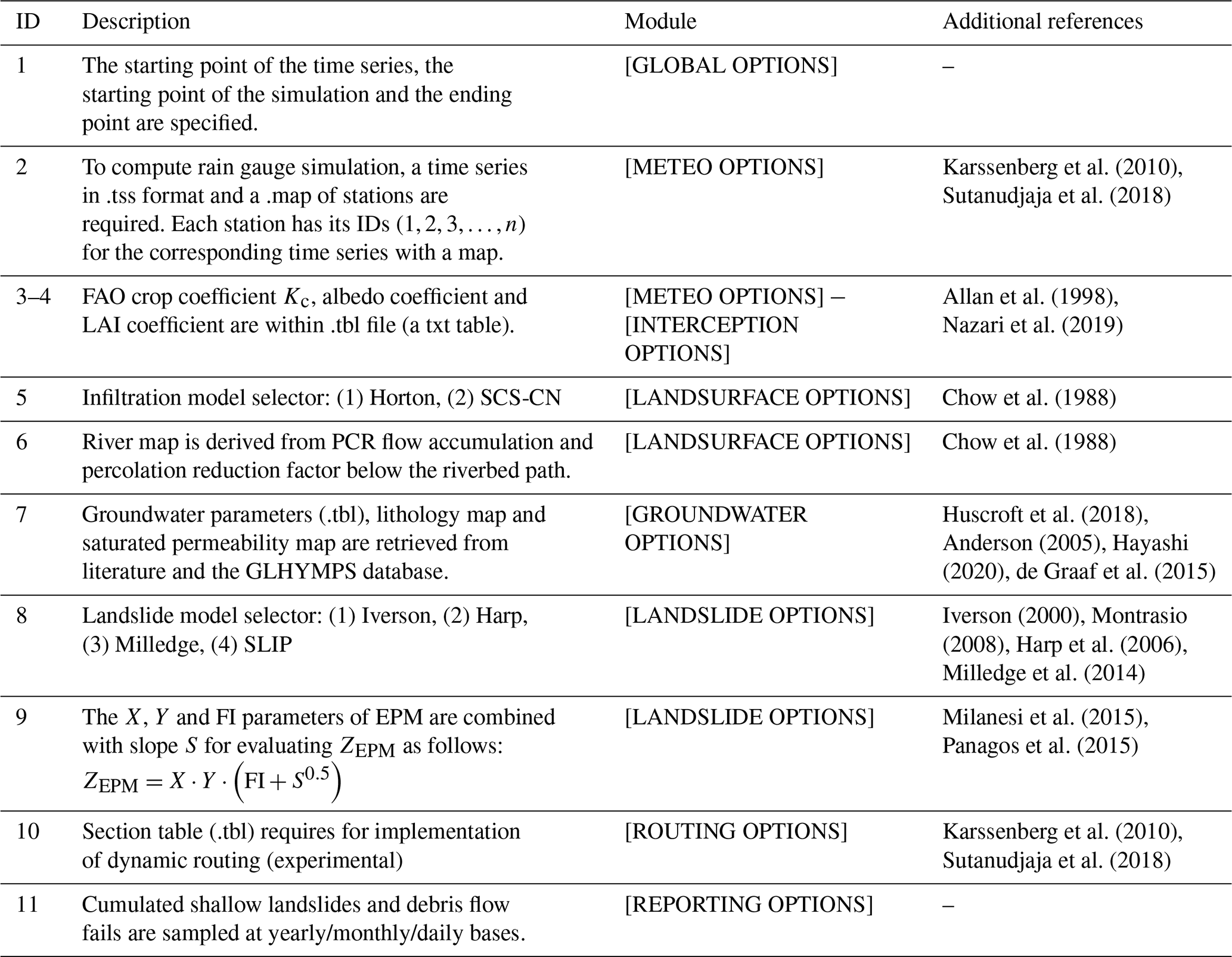
In this section, main symbols and their measurement units included in CRHyME are reported (Abbate and Mancusi, 2021a, b).
Table B1List of the symbols adopted for variables and parameters in the CRHyME model.
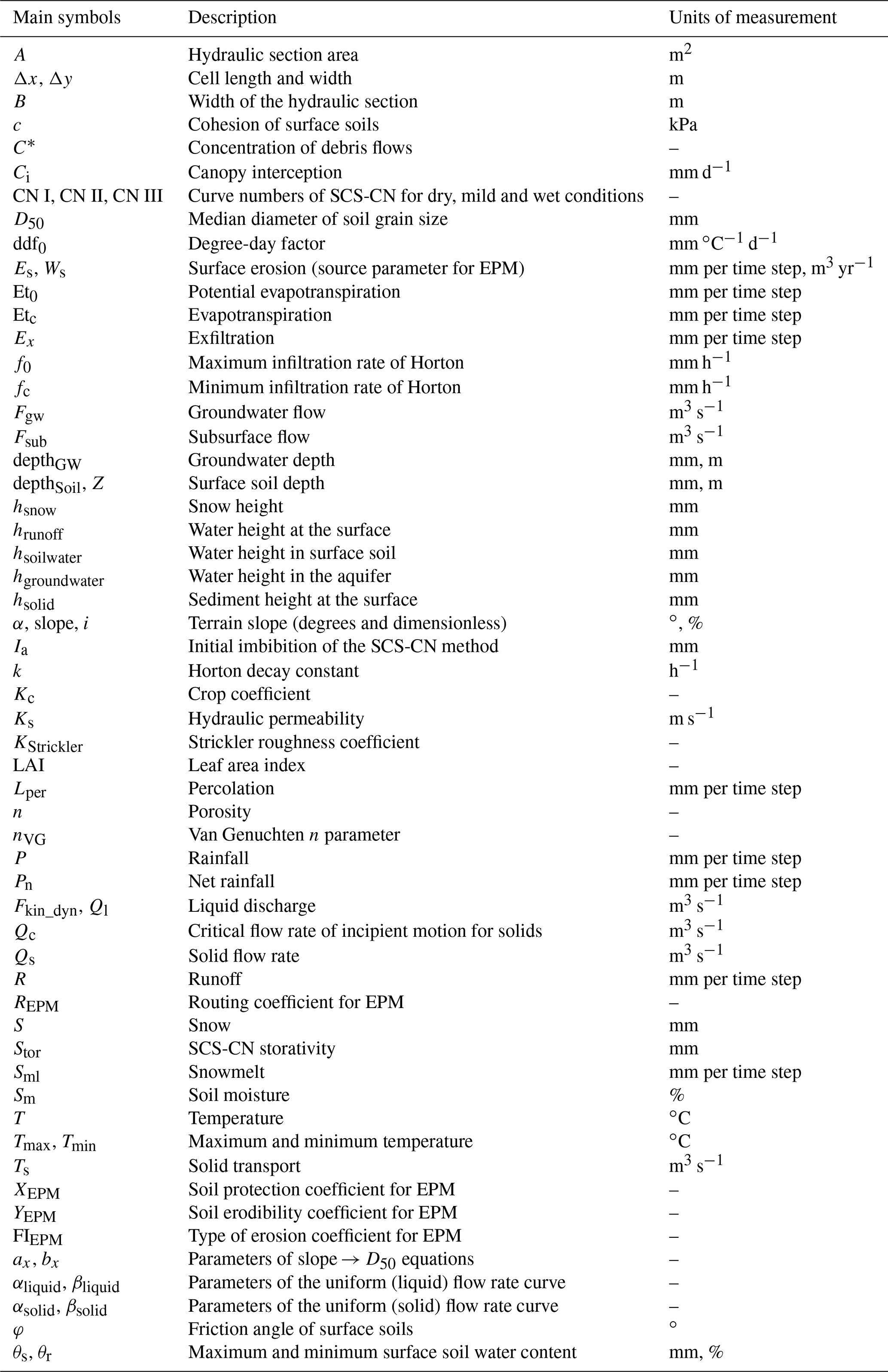
All the data shown in this paper are freely consultable on internet websites as reported in Sect. 2.2.1 (CORINE, SoilGrids, HydroSHEDS, ESDAC, ARPA Emilia-Romagna and ARPA Lombardia). Since the CRHyME code is currently underdeveloped, we suggest you contact the main author at andrea.abbate@rse-web.it to receive the most updated and stable copy of the code. To use the code, CRHyME requires a Python environment (we suggest Python 3.7 or 3.8) and the installation of PCRaster libraries (see Karssenberg et al., 2010 and links). Further details can be found in Abbate and Mancusi (2021a, b).
AA and LM conceptualized the study. AA carried out the formal analysis and wrote the manuscript with contributions from all co-authors. FA, AF, LL and MP supervised the research, and all the authors reviewed and edited the manuscript.
The contact author has declared that none of the authors has any competing interests.
Publisher's note: Copernicus Publications remains neutral with regard to jurisdictional claims made in the text, published maps, institutional affiliations, or any other geographical representation in this paper. While Copernicus Publications makes every effort to include appropriate place names, the final responsibility lies with the authors.
This article is part of the special issue “Hydro-meteorological extremes and hazards: vulnerability, risk, impacts, and mitigation”. It is a result of the European Geosciences Union General Assembly 2022, Vienna, Austria, 23–27 May 2022.
This work has been financed by the research fund of the Italian electrical system under the 3-year research plan for 2022–2024 (DM MITE no. 337, 15 September 2022), in compliance with the decree of 16 April 2018.
This paper was edited by Francesco Marra and reviewed by Evren Soylu and two anonymous referees.
Abbate, A. and Mancusi, L.: Manuale del modello CRHyME (Climate Rainfall Hydrogeological Modelling Experiment), RSE Report RdS 21012462, Milano, RSE , https://www.rse-web.it/rapporti/manuale-del-modello-crhyme-climatic-rainfall-hydrogeological (last access: 1 November 3)202, 2021a.
Abbate, A. and Mancusi, L.: Strumenti per la mappatura delle minacce idrogeologiche per il sistema energetico e incidenza dei cambiamenti climatici, RSE Report RdS 21010317, Milano, RSE, https://www.rse-web.it/rapporti/strumenti-per-la-mappatura-delle-minacce-idrogeologiche-per (last access: 1 November 2023), 2021b.
Abbate, A., Longoni, L., Ivanov, V. I., and Papini, M.: Wildfire impacts on slope stability triggering in mountain areas, MDPI Geosci., 9, 1–15, https://doi.org/10.3390/geosciences9100417, 2019.
Abbate, A., Papini, M., and Longoni, L.: Analysis of meteorological parameters triggering rainfall-induced landslide: a review of 70 years in Valtellina, Nat. Hazards Earth Syst. Sci., 21, 2041–2058, https://doi.org/10.5194/nhess-21-2041-2021, 2021a.
Abbate, A., Papini, M., and Longoni, L.: Extreme Rainfall over Complex Terrain: An Application of the Linear Model of Orographic Precipitation to a Case Study in the Italian Pre-Alps, Geosciences, 11, 18, https://doi.org/10.3390/geosciences11010018, 2021b.
Abeshu, G. W., Li, H.-Y., Zhu, Z., Tan, Z., and Leung, L. R.: Median bed-material sediment particle size across rivers in the contiguous US, Earth Syst. Sci. Data, 14, 929–942, https://doi.org/10.5194/essd-14-929-2022, 2022.
Allan, R., Pereira, L., and Smith, M.: Crop evapotranspiration-Guidelines for computing crop water requirements – FAO Irrigation and drainage paper 56, FAO, https://www.fao.org/3/X0490E/x0490e00.htm (last access: 1 November 2023) 1998.
Alvioli, M., Melillo, M., Guzzetti, F., Rossi, M., Palazzi, E., von Hardenberg, J., Brunetti, M. T., and Peruccacci, S.: Implications of climate change on landslide hazard in Central Italy, Sci. Total Environ., 630, 1528–1543, https://doi.org/10.1016/j.scitotenv.2018.02.315, 2018.
Ancey, C.: Bedload transport: a walk between randomness and determinism. Part 1. The state of the art, J. Hydraul. Res., 58, 1–17, https://doi.org/10.1080/00221686.2019.1702594, 2020.
Anderson, E. I.: Modeling groundwater–surface water interactions using the Dupuit approximation, Adv. Water Resour., 28, 315–327, https://doi.org/10.1016/j.advwatres.2004.11.007, 2005.
Angeli, M. G., Buma, J., Gasparetto, P., and Pasuto, A.: A combined hill slope hydrology/stability model for low-gradient slopes in the Italian Dolomites, Eng. Geol., 49, 1–13, https://doi.org/10.1016/S0013-7952(97)00033-1, 1998.
Autorità di Bacino Distrettuale del Fiume Po: Linee Generali di Assetto Idrogeologico e Quadro degli Interventi, https://pai.adbpo.it/index.php/documentazione-pai/ (last access: 1 November 2023), 2022.
Ballio, F., Brambilla, D., Giorgetti, E., Longoni, L., Papini, M., and Radice, A.: Evaluation of sediment yield from valley slopes: A case study, WIT Trans. Eng. Sci., 67, 149–160, https://doi.org/10.2495/DEB100131, 2010.
Bancheri, M., Rigon, R., and Manfreda, S.: The GEOframe-NewAge Modelling System Applied in a Data Scarce Environment, Water, 12, 86, https://doi.org/10.3390/w12010086, 2020.
Barnes, R.: Parallel Priority-Flood depression filling for trillion cell digital elevation models on desktops or clusters, Comput. Geosci., 96, 56–68, https://doi.org/10.1016/j.cageo.2016.07.001, 2016.
Barnes, R.: Parallel non-divergent flow accumulation for trillion cell digital elevation models on desktops or clusters, Environ. Model. Softw., 92, 202–212, https://doi.org/10.1016/j.envsoft.2017.02.022, 2017.
Bemporad, G. A., Alterach, J., Amighetti, F. F., Peviani, M., and Saccardo, I.: A distributed approach for sediment yield evaluation in Alpine regions, J. Hydrol., 197, 370–392, https://doi.org/10.1016/0022-1694(95)02978-8, 1997.
Berg, J. H.: Prediction of Alluvial Channel Pattern of Perennial Rivers, Geomorphology, 12, 259–279, https://doi.org/10.1016/0169-555X(95)00014-V, 1995.
Bonanno, R., Lacavalla, M., and Sperati, S.: A new high-resolution Meteorological Reanalysis Italian Dataset: MERIDA, Q. J. Roy. Meteorol. Soc., 145, 1756–1779, https://doi.org/10.1002/qj.3530, 2019.
Bordoni, M., Meisina, C., Valentino, R., Lu, N., Bittelli, M., and Chersich, S.: Hydrological factors affecting rainfall-induced shallow landslides: From the field monitoring to a simplified slope stability analysis, Eng. Geol., 193, 19–37, https://doi.org/10.1016/j.enggeo.2015.04.006, 2015.
Bovolo, C. I. and Bathurst, J. C.: Modelling catchment-scale shallow landslide occurrence and sediment yield as a function of rainfall return period, Hydrol. Process., 26, 579–596, https://doi.org/10.1002/hyp.8158, 2012.
Bovy, B., Braun, J., Cordonnier, G., Lange, R., and Yuan, X.: The FastScape software stack: reusable tools for landscape evolution modelling, EGU General Assembly 2020, Online, 4–8 May 2020, EGU2020-9474, https://doi.org/10.5194/egusphere-egu2020-9474, 2020.
Bozzolan, E., Holcombe, E., Pianosi, F., and Wagener, T.: Including informal housing in slope stability analysis – an application to a data-scarce location in the humid tropics, Nat. Hazards Earth Syst. Sci., 20, 3161–3177, https://doi.org/10.5194/nhess-20-3161-2020, 2020.
Brambilla, D., Papini, M., Ivanov, V. I., Bonaventura, L., Abbate, A., and Longoni, L.: Sediment Yield in Mountain Basins, Analysis, and Management: The SMART-SED Project, in: Applied Geology: Approaches to Future Resource Management, edited by: De Maio, M. and Tiwari, A. K., Springer International Publishing, Cham, 43–59, https://doi.org/10.1007/978-3-030-43953-8_3, 2020.
Bresciani, E., Davy, P., and de Dreuzy, J.-R.: Is the Dupuit assumption suitable for predicting the groundwater seepage area in hillslopes?, Water Resour. Res., 50, 2394–2406, https://doi.org/10.1002/2013WR014284, 2014.
Campforts, B., Shobe, C. M., Steer, P., Vanmaercke, M., Lague, D., and Braun, J.: HyLands 1.0: a hybrid landscape evolution model to simulate the impact of landslides and landslide-derived sediment on landscape evolution, Geosci. Model Dev., 13, 3863–3886, https://doi.org/10.5194/gmd-13-3863-2020, 2020.
Cazorzi, F. and Dalla Fontana, G.: Snowmelt modelling by combining air temperature and a distributed radiation index, J. Hydrol., 181, 169–187, https://doi.org/10.1016/0022-1694(95)02913-3, 1996.
Ceriani, M., Lauzi, S., and Padovan, M.: Rainfall thresholds triggering debris-flow in the alpine area of Lombardia Region, central Alps – Italy, in: Proceedings of the Man and Mountain'94, First International Congress for the Protection and Development of Mountain Environmen, 20–24 June 1994, Ponte di Legno, BS, Italy, 1994.
Chen, L. and Young, M. H.: Green-Ampt infiltration model for sloping surfaces, Water Resour. Res., 42, W07420, https://doi.org/10.1029/2005WR004468, 2006.
Chiarelli, D. D., Galizzi, M., Bocchiola, D., Rosso, R., and Rulli, M. C.: Modeling snowmelt influence on shallow landslides in Tartano valley, Italian Alps, Sci. Total Environ., 856, 158772, https://doi.org/10.1016/j.scitotenv.2022.158772, 2023.
Chow, V. T., Maidment, D. R., and Mays, L. W.: Applied hydrology, McGraw-Hill, New York, ISBN 007070242X, ISBN 9780070702424, 1988.
Ciampalini, A., Raspini, F., Lagomarsino, D., Catani, F., and Casagli, N.: Landslide susceptibility map refinement using PSInSAR data, Remote Sens. Environ., 184, 302–315, https://doi.org/10.1016/j.rse.2016.07.018, 2016.
Ciccarese, G., Mulas, M., Alberoni, P. P., Truffelli, G., and Corsini, A.: Debris flows rainfall thresholds in the Apennines of Emilia-Romagna (Italy) derived by the analysis of recent severe rainstorms events and regional meteorological data, Geomorphology, 358, 107097, https://doi.org/10.1016/j.geomorph.2020.107097, 2020.
Ciccarese, G., Mulas, M., and Alessandro, C.: Combining spatial modelling and regionalization of rainfall thresholds for debris flows hazard mapping in the Emilia-Romagna Apennines (Italy), Landslides, 18, 1–17, https://doi.org/10.1007/s10346-021-01739-w, 2021.
Cislaghi, A., Chiaradia, E. A., and Bischetti, G. B.: Including root reinforcement variability in a probabilistic 3D stability model, Earth Surf. Proc. Land., 42, 1789–1806, https://doi.org/10.1002/esp.4127, 2017.
CNR and IRPI: Rapporto Periodico sul Rischio posto alla Popolazione italiana da Frane e Inondazioni, Anno 2020, 19 pp., https://doi.org/10.30437/report2020, 2021.
Collischonn, W., Fleischmann, A., Paiva, R. C. D., and Mejia, A.: Hydraulic Causes for Basin Hydrograph Skewness, Water Resour. Res., 53, 10603–10618, https://doi.org/10.1002/2017WR021543, 2017.
Crosta, G. B. and Frattini, P.: Distributed modelling of shallow landslides triggered by intense rainfall, Nat. Hazards Earth Syst. Sci., 3, 81–93, https://doi.org/10.5194/nhess-3-81-2003, 2003.
Crosta, G. B., Imposimato, S., and Roddeman, D. G.: Numerical modelling of large landslides stability and runout, Nat. Hazards Earth Syst. Sci., 3, 523–538, https://doi.org/10.5194/nhess-3-523-2003, 2003.
Dade, W. B. and Friend, P. F.: Grain-Size, Sediment-Transport Regime, and Channel Slope in Alluvial Rivers, J. Geol., 106, 661–676, https://doi.org/10.1086/516052, 1998.
D'Agostino, V. and Marchi, L.: Debris flow magnitude in the Eastern Italian Alps: Data collection and analysis, Phys. Chem. Earth Pt. C, 26, 657–663, https://doi.org/10.1016/S1464-1917(01)00064-2, 2001.
Daly, C., Taylor, G., and Gibson, W.: The PRISM Approach to Mapping Precipitation and Temperature, https://api.semanticscholar.org/CorpusID:17141237 (last access: 1 November 2023), 1997.
Daly, C., Slater, M. E., Roberti, J. A., Laseter, S. H., and Swift Jr., L. W.: High-resolution precipitation mapping in a mountainous watershed: ground truth for evaluating uncertainty in a national precipitation dataset, Int. J. Climatol., 37, 124–137, https://doi.org/10.1002/joc.4986, 2017.
Davolio, S., Della Fera, S., Laviola, S., Miglietta, M. M., and Levizzani, V.: Heavy precipitation over Italy from the Mediterranean storm “Vaia” in October 2018: Assessing the role of an atmospheric river, Mon. Weather Rev., 148, 3571–3588, 2020.
Davy, P. and Lague, D.: Fluvial erosion/transport equation of landscape evolution models revisited, J. Geophys. Res.-Earth, 114, F03007, https://doi.org/10.1029/2008JF001146, 2009.
de Graaf, I. E. M., Sutanudjaja, E. H., van Beek, L. P. H., and Bierkens, M. F. P.: A high-resolution global-scale groundwater model, Hydrol. Earth Syst. Sci., 19, 823–837, https://doi.org/10.5194/hess-19-823-2015, 2015.
de Vente, J. and Poesen, J.: Predicting soil erosion and sediment yield at the basin scale: Scale issues and semi-quantitative models, Earth-Sci. Rev., 71, 95–125, https://doi.org/10.1016/j.earscirev.2005.02.002, 2005.
Devia, G. K., Ganasri, B. P., and Dwarakish, G. S.: A Review on Hydrological Models, Aquat. Proced., 4, 1001–1007, https://doi.org/10.1016/j.aqpro.2015.02.126, 2015.
De Vita, P., Fusco, F., Tufano, R., and Cusano, D.: Seasonal and Event-Based Hydrological and Slope Stability Modeling of Pyroclastic Fall Deposits Covering Slopes in Campania (Southern Italy), Water, 10, 1140, https://doi.org/10.3390/w10091140, 2018.
D'Odorico, P. and Fagherazzi, S.: A probabilistic model of rainfall-triggered shallow landslides in hollows: A long-term analysis, Water Resour. Res., 39, 1262, https://doi.org/10.1029/2002WR001595, 2003.
Erskine, R. H., Green, T. R., Ramirez, J. A., and MacDonald, L. H.: Comparison of grid-based algorithms for computing upslope contributing area, Water Resour. Res., 42, W09416, https://doi.org/10.1029/2005WR004648, 2006.
Fan, Y., Miguez-Macho, G., Weaver, C. P., Walko, R., and Robock, A.: Incorporating water table dynamics in climate modeling: 1. Water table observations and equilibrium water table simulations, J. Geophys. Res.-Atmos., 112, D10125, https://doi.org/10.1029/2006JD008111, 2007.
Fawcett, T.: An introduction to ROC analysis, Pattern Recog. Lett., 27, 861–874, https://doi.org/10.1016/j.patrec.2005.10.010, 2006.
Formetta, G., Capparelli, G., and Versace, P.: Evaluating performance of simplified physically based models for shallow landslide susceptibility, Hydrol. Earth Syst. Sci., 20, 4585–4603, https://doi.org/10.5194/hess-20-4585-2016, 2016.
Gao, L., Zhang, L. M., and Cheung, R. W. M.: Relationships between natural terrain landslide magnitudes and triggering rainfall based on a large landslide inventory in Hong Kong, Landslides, 15, 727–740, https://doi.org/10.1007/s10346-017-0904-x, 2018.
Gariano, S. L. and Guzzetti, F.: Landslides in a changing climate, Earth-Sci. Rev., 162, 227–252, https://doi.org/10.1016/j.earscirev.2016.08.011, 2016.
GDAL/OGR contributors: GDAL/OGR Geospatial Data Abstraction software Library, Open Source Geospatial Foundation, https://gdal.org/index.html (last access: 1 November 2023), 2020.
Girard, M.-C., Girard, C., Dominique, C., Gilliot, J.-M., Loubersac, L., Meyer-Roux, J., Monget, J.-M., Seguin, B., and Rao, N.: Corine Land Cover, Routledge, 331–344, https://doi.org/10.1201/9780203741917-19, 2018.
Gleick, P. H.: Climate change, hydrology, and water resources, Rev. Geophys., 27, 329–344, https://doi.org/10.1029/RG027i003p00329, 1989.
Globevnik, L., Holjević, D., Petkovšek, G., and Rubinić, J.: 145. Applicability of the Gavrilo vic Method in Erosion Calculation Using Spatial Data Manipulation Techniques, Tunnelling and Underground Space Technology, 14 pp. https://api.semanticscholar.org/CorpusID:54749986 (last access: 1 November 2023), 2003.
Govers, G.: Empirical relationships for the transport capacity of overland flow, https://iahs.info/uploads/dms/8088.45-63-189-Govers.pdf (last access: 1 November 2023), 1989.
Govers, G., Wallings, D. E., Yair, A., and Berkowicz, S.: Empirical relationships for the transport capacity of overland flow, International Association of Hydrological Sciences, 189 pp., 1990.
Groenendyk, D. G., Ferré, T. P. A., Thorp, K. R., and Rice, A. K.: Hydrologic-Process-Based Soil Texture Classifications for Improved Visualization of Landscape Function., PLoS One, 10, e0131299, https://doi.org/10.1371/journal.pone.0131299, 2015.
Guadagno, M., Guzzetti, I., Reichenbach, I., and Tonelli, I.: SICI – Sistema Informativo Catastrofi Idrogeologiche, Istituto di Ricerca per la Protezione Idrogeologica (IRPI) del Consiglio Nazionale delle Ricerche e Gruppo Nazionale per la Difesa dalle Catastrofi Idrogeologiche (GNDCI) del Consiglio Nazionale delle Ricerche, https://sici.irpi.cnr.it/ (last access: 1 November 2023), 2003.
Gudiyangada Nachappa, T., Tavakkoli Piralilou, S., Ghorbanzadeh, O., Shahabi, H., and Blaschke, T.: Landslide Susceptibility Mapping for Austria Using Geons and Optimization with the Dempster-Shafer Theory, Appl. Sci., 9, 5393, https://doi.org/10.3390/app9245393, 2019.
Guzzetti, F. and Tonelli, G.: Information system on hydrological and geomorphological catastrophes in Italy (SICI): a tool for managing landslide and flood hazards, Nat. Hazards Earth Syst. Sci., 4, 213–232, https://doi.org/10.5194/nhess-4-213-2004, 2004.
Guzzetti, F., Reichenbach, P., Cardinali, M., Galli, M., and Ardizzone, F.: Probabilistic landslide hazard assessment at the basin scale, Geomorphology, 72, 272–299, https://doi.org/10.1016/j.geomorph.2005.06.002, 2005.
Guzzetti, F., Peruccacci, S., Rossi, M., and Stark, C. P.: Rainfall thresholds for the initiation of landslides in central and southern Europe, Meteorol. Atmos. Phys., 98, 239–267, https://doi.org/10.1007/s00703-007-0262-7, 2007.
Harp, E. L., Michael, J. A., and Laprade, W. T.: Shallow-landslide hazard map of Seattle, USGS, Washington, Reston, VA, https://doi.org/10.3133/ofr20061139, 2006.
Hayashi, M.: Alpine Hydrogeology: The Critical Role of Groundwater in Sourcing the Headwaters of the World, Groundwater, 58, 498–510, https://doi.org/10.1111/gwat.12965, 2020.
Hengl, T., Mendes de Jesus, J., Heuvelink, G. B. M., Ruiperez Gonzalez, M., Kilibarda, M., Blagotić, A., Shangguan, W., Wright, M. N., Geng, X., Bauer-Marschallinger, B., Guevara, M. A., Vargas, R., MacMillan, R. A., Batjes, N. H., Leenaars, J. G. B., Ribeiro, E., Wheeler, I., Mantel, S., and Kempen, B.: SoilGrids250m: Global gridded soil information based on machine learning, PLOS ONE, 12, e0169748, https://doi.org/10.1371/journal.pone.0169748, 2017.
Herrera, M.: Landslide Detection using Random Forest Classifier, Delft University of Technology, Delft, https://doi.org/10.13140/RG.2.2.31365.91369, 2019.
Huscroft, J., Gleeson, T., Hartmann, J., and Börker, J.: Compiling and Mapping Global Permeability of the Unconsolidated and Consolidated Earth: GLobal HYdrogeology MaPS 2.0 (GLHYMPS 2.0), Geophys. Res. Lett., 45, 1897–1904, https://doi.org/10.1002/2017GL075860, 2018.
Iida, T.: A stochastic hydro-geomorphological model for shallow landsliding due to rainstorm, Catena, 34, 293–313, https://doi.org/10.1016/S0341-8162(98)00093-9, 1999.
ISPRA: Dissesto idrogeologico in Italia: pericolosità e indicatori di rischio, Ispra, https://www.isprambiente.gov.it/it/attivita/suolo-e-territorio/dissesto-idrogeologico (last access: 1 November 2023), 2018.
ITCOLD: La gestione dell'interrimento dei serbatoi artificiali italiani, Comitato Nazionale Italiano delle Grandi Dighe, https://www.itcold.it/wpsysfiles/wp-content/uploads/2016/07/RAPPFIN-GdLInterrimento-Fase1-20091.pdf (last access: 1 November 2023), 2009.
ITCOLD: La gestione dell'interrimento dei serbatoi artificiali italiani situazione attuale e prospettive, Comitato Nazionale Italiano delle Grandi Dighe, https://www.itcold.it/wpsysfiles/wp-content/uploads/2016/07/RAPPFIN-GdLInterrimento-Fase2-20092.pdf (last access: 1 November 2023), 2016.
Ivanov, V., Radice, A., Papini, M., and Longoni, L.: Event-scale pebble mobility observed by RFID tracking in a pre-Alpine stream: a field laboratory, Earth Surf. Proc. Land., 45, 535–547, https://doi.org/10.1002/esp.4752, 2020a.
Ivanov, V., Arosio, D., Tresoldi, G., Hojat, A., Zanzi, L., Papini, M., and Longoni, L.: Investigation on the Role of Water for the Stability of Shallow Landslides-Insights from Experimental Tests, Water, 12, 1203, https://doi.org/10.3390/w12041203, 2020b.
Iverson, R., Reid, M., and Lahusen, R.: Debris-flow mobilization from landslides. Annu Rev Earth Planet Sci, Annu. Rev. Earth Planet. Sci., 25, 85–138, https://doi.org/10.1146/annurev.earth.25.1.85, 1997.
Iverson, R. M.: Landslide triggering by rain infiltration, Water Resour. Res., 36, 1897–1910, https://doi.org/10.1029/2000WR900090, 2000.
Jackson, C. R., Bitew, M., and Du, E.: When interflow also percolates: downslope travel distances and hillslope process zones, Hydrol. Process., 28, 3195–3200, https://doi.org/10.1002/hyp.10158, 2014.
Jacob, D., Petersen, J., Eggert, B., Alias, A., Christensen, O. B., Bouwer, L. M., Braun, A., Colette, A., Déqué, M., Georgievski, G., Georgopoulou, E., Gobiet, A., Menut, L., Nikulin, G., Haensler, A., Hempelmann, N., Jones, C., Keuler, K., Kovats, S., Kröner, N., Kotlarski, S., Kriegsmann, A., Martin, E., van Meijgaard, E., Moseley, C., Pfeifer, S., Preuschmann, S., Radermacher, C., Radtke, K., Rechid, D., Rounsevell, M., Samuelsson, P., Somot, S., Soussana, J.-F., Teichmann, C., Valentini, R., Vautard, R., Weber, B., and Yiou, P.: EURO-CORDEX: new high-resolution climate change projections for European impact research, Reg. Environ. Change, 14, 563–578, https://doi.org/10.1007/s10113-013-0499-2, 2014.
Jakob, M. and Hungr, O.: Debris-Flow Hazards and Related Phenomena, Springer, ISBN 978-3-540-20726-9, 2005.
Jakob, M. and Jordan, P.: Design flood estimates in mountain streams – the need for a geomorphic approach, Can. J. Civ. Eng., 28, 425–439, https://doi.org/10.1139/l01-010, 2001.
Kadavi, P., Lee, C.-W., and Lee, S.: Application of Ensemble-Based Machine Learning Models to Landslide Susceptibility Mapping, Remote Sens., 10, 1252, https://doi.org/10.3390/rs10081252, 2018.
Karssenberg, D., Schmitz, O., Salamon, P., de Jong, K., and Bierkens, M. F. P.: A software framework for construction of process-based stochastic spatio-temporal models and data assimilation, Environ. Model. Softw., 25, 489–502, https://doi.org/10.1016/j.envsoft.2009.10.004, 2010.
Kim, K.-S., Kim, M.-I., Lee, M.-S., and Hwang, E.-S.: Regression Equations for Estimating Landslide-Triggering Factors Using Soil Characteristics, Appl. Sci., 10, 3560, https://doi.org/10.3390/app10103560, 2020.
Klaus, J. and Jackson, C. R.: Interflow Is Not Binary: A Continuous Shallow Perched Layer Does Not Imply Continuous Connectivity, Water Resour. Res., 54, 5921–5932, https://doi.org/10.1029/2018WR022920, 2018.
Kobierska, F., Jonas, T., Kirchner, J. W., and Bernasconi, S. M.: Linking baseflow separation and groundwater storage dynamics in an alpine basin (Dammagletscher, Switzerland), Hydrol. Earth Syst. Sci., 19, 3681–3693, https://doi.org/10.5194/hess-19-3681-2015, 2015.
Kondolf, G. M.: Hungry Water: Effects of Dams and Gravel Mining on River Channels, Environ. Manage., 21, 533–551, https://doi.org/10.1007/s002679900048, 1997.
Lamb, M. P. and Venditti, J. G.: The grain size gap and abrupt gravel-sand transitions in rivers due to suspension fallout, Geophys. Res. Lett., 43, 3777–3785, https://doi.org/10.1002/2016GL068713, 2016.
Langland, M. J.: Bathymetry and Sediment-Storage Capacity Change in Three Reservoirs on the Lower Susquehanna River, 1996–2008, USGS, https://doi.org/10.3133/sir20095110, 2009.
Lazzari, M., Piccarreta, M., and Manfreda, S.: The role of antecedent soil moisture conditions on rainfall-triggered shallow landslides, Nat. Hazards Earth Syst. Sci. Discuss. [preprint], https://doi.org/10.5194/nhess-2018-371, 2018.
Lee, K. and Pin Chun, H.: Evaluating the adequateness of kinematic-wave routing for flood forecasting in midstream channel reaches of Taiwan, J. Hydroinform., 14, 1075, https://doi.org/10.2166/hydro.2012.093, 2012.
Legorreta Paulin, G., Bursik, M., Lugo-Hubp, J., and Zamorano Orozco, J. J.: Effect of pixel size on cartographic representation of shallow and deep-seated landslide, and its collateral effects on the forecasting of landslides by SINMAP and Multiple Logistic Regression landslide models, Phys. Chem. Earth Pt. A/B/C, 35, 137–148, https://doi.org/10.1016/j.pce.2010.04.008, 2010.
Lehner, B., Verdin, K., and Jarvis, A.: New Global Hydrography Derived From Spaceborne Elevation Data, Eos Trans. Am. Geophys. Union, 89, 93–94, https://doi.org/10.1029/2008EO100001, 2008.
Li, X., Xiao, Q., Niu, J., Dymond, S., McPherson, E. G., van Doorn, N., Yu, X., Xie, B., Zhang, K., and Li, J.: Rainfall interception by tree crown and leaf litter: An interactive process, Hydrol. Process., 31, 3533–3542, https://doi.org/10.1002/hyp.11275, 2017.
Longoni, L., Ivanov, V. I., Brambilla, D., Radice, A., and Papini, M.: Analysis of the temporal and spatial scales of soil erosion and transport in a Mountain Basin, Ital. J. Eng. Geol. Environ., 16, 17–30, https://doi.org/10.4408/IJEGE.2016-02.O-02, 2016.
López Vicente, M., Pérez-Bielsa, C., López-Montero, T., Lambán, L. J., and Navas, A.: Runoff simulation with eight different flow accumulation algorithms: Recommendations using a spatially distributed and open-source model, Environ. Model. Softw., 62, 11–21, 2014.
Luino, F.: Sequence of instability processes triggered by heavy rainfall in the Northern Italy, Geomorphology, 66, 13–39, https://doi.org/10.1016/j.geomorph.2004.09.010, 2005.
Ly, S., Charles, C., and Degre, A.: Different methods for spatial interpolation of rainfall data for operational hydrology and hydrological modeling at watershed scale. A review, Biotechnol. Agron. Soc. Environ., 17, 392–406, 2013.
Marnezy, A.: Alpine dams. From hydroelectric power to artificial snow, Revue De Geographie Alpine – Journal of Alpine Research, 96, 103–112, 2008.
Meisina, C., Zizioli, D., and Zucca, F.: Methods for shallow landslides susceptibility mapping: an example in Oltrepo Pavese (Northern Italy), Landslides Science and Practice, in: Volume 1: Landslide Inventory and Susceptibility and Hazard, edited by: Zoning Margottini, C., Canuti, P., and Sassa, K., Springer, 451–458, ISBN 978-3-642-31324-0, https://doi.org/10.1007/978-3-642-31325-7, 2013.
Merritt, W. S., Letcher, R. A., and Jakeman, A. J.: A review of erosion and sediment transport models, Environ. Model. Softw., 18, 761–799, https://doi.org/10.1016/S1364-8152(03)00078-1, 2003.
Michel, G. P., Kobiyama, M., and Goerl, R. F.: Comparative analysis of SHALSTAB and SINMAP for landslide susceptibility mapping in the Cunha River basin, southern Brazil, J. Soils Sediments, 14, 1266–1277, https://doi.org/10.1007/s11368-014-0886-4, 2014.
Milanesi, L., Pilotti, M., Clerici, A., and Gavrilovic, Z.: Application of an improved version of the Erosion Potential Method in Alpine areas, Ital. J. Eng. Geol. Environ., 1, 17–30, https://doi.org/10.4408/IJEGE.2015-01.O-02, 2015.
Milledge, D. G., Bellugi, D., McKean, J. A., Densmore, A. L., and Dietrich, W. E.: A multidimensional stability model for predicting shallow landslide size and shape across landscapes, J. Geophys. Res.-Earth, 119, 2481–2504, https://doi.org/10.1002/2014JF003135, 2014.
Mishra, S. K., Tyagi, J. V., and Singh, V. P.: Comparison of infiltration models, Hydrol. Process., 17, 2629–2652, https://doi.org/10.1002/hyp.1257, 2003.
Moges, E., Demissie, Y., Larsen, L., and Yassin, F.: Review: Sources of Hydrological Model Uncertainties and Advances in Their Analysis, Water, 13, 28, https://doi.org/10.3390/w13010028, 2021.
Montrasio, L.: Stability of soil-slip, Risk Analysis II, WIT Press, https://www.witpress.com/Secure/elibrary/papers/RISK00/RISK00033FU.pdf (last access: 1 November 2023), 2008.
Montrasio, L. and Valentino, R.: Modelling Rainfall-induced Shallow Landslides at Different Scales Using SLIP – Part II, Proced. Eng., 158, 482–486, https://doi.org/10.1016/j.proeng.2016.08.476, 2016.
Morbidelli, R., Corradini, C., Saltalippi, C., Flammini, A., Dari, J., and Govindaraju, R. S.: Rainfall Infiltration Modeling: A Review, Water, 10, 1873, https://doi.org/10.3390/w10121873, 2018.
Morgan, R. P. C. and Nearing, M. A. (Eds.): Handbook of erosion modelling, Blackwell Publishing Ltd, ISBN 9781405190107, ISBN 9781444328455, https://doi.org/10.1002/9781444328455, 2011.
Munich Re: Natural disasters caused overall losses of US $ 210bn Relevant natural catastrophe loss events worldwide 2020, https://www.munichre.com/content/dam/munichre/mrwebsiteslaunches/natcat-2021/2020_Jan-Dec_Weltkarte_e.pdf/_jcr_content/renditions/original./2020_Jan-Dec_Weltkarte_e.pdf (last access: 1 November 2023), 2021.
Nazari, M., Sadeghi, S. M. M., Van Stan, J., and Chaichi, M.: Rainfall interception and redistribution by maize farmland in central Iran, J. Hydrol.: Reg. Stud., 27, 100656, https://doi.org/10.1016/j.ejrh.2019.100656, 2019.
Nino, Y.: Simple Model for Downstream Variation of Median Sediment Size in Chilean Rivers, J. Hydraul. Eng., 128, 934–941, 2002.
Oguz, E. A., Depina, I., and Thakur, V.: Effects of soil heterogeneity on susceptibility of shallow landslides, Landslides, 19, 67–83, https://doi.org/10.1007/s10346-021-01738-x, 2022.
Pacina, J., Lenďáková, Z., Štojdl, J., Matys Grygar, T., and Dolejš, M.: Dynamics of Sediments in Reservoir Inflows: A Case Study of the Skalka and Nechranice Reservoirs, Czech Republic, ISPRS Int. J. Geo-Inform., 9, 258, https://doi.org/10.3390/ijgi9040258, 2020.
Panagos, P., Borrelli, P., Poesen, J., Ballabio, C., Lugato, E., Meusburger, K., Montanarella, L., and Alewell, C.: The new assessment of soil loss by water erosion in Europe, Environ. Sci. Policy, 54, 438–447, https://doi.org/10.1016/j.envsci.2015.08.012, 2015.
Papini, M., Ivanov, V., Brambilla, D., Arosio, D., and Longoni, L.: Monitoring bedload sediment transport in a pre-Alpine river: An experimental method, Rendiconti Online della Società Geologica Italiana, 43, 57–63, https://doi.org/10.3301/ROL.2017.35, 2017.
Parenti, C., Rossi, P., Mancini, F., Scorpio, V., Grassi, F., Ciccarese, G., Lugli, F., and Soldati, M.: Multitemporal Analysis of Slow-Moving Landslides and Channel Dynamics through Integrated Remote Sensing and In Situ Techniques, Remote Sens., 15, 3563, https://doi.org/10.3390/rs15143563, 2023.
Pearson, E., Smith, M. W., Klaar, M. J., and Brown, L. E.: Can high resolution 3D topographic surveys provide reliable grain size estimates in gravel bed rivers?, Geomorphology, 293, 143–155, https://doi.org/10.1016/j.geomorph.2017.05.015, 2017.
Pebesma, E. J., de Jong, K., and Briggs, D.: Interactive visualization of uncertain spatial and spatio-temporal data under different scenarios: an air quality example, Int. J. Geogr. Inform. Sci., 21, 515–527, https://doi.org/10.1080/13658810601064009, 2007.
Peirce, S., Ashmore, P., and Leduc, P.: Evolution of grain size distributions and bed mobility during hydrographs in gravel-bed braided rivers, Earth Surf. Proc. Land., 44, 304–316, https://doi.org/10.1002/esp.4511, 2019.
Pelletier, J. D., Broxton, P. D., Hazenberg, P., Zeng, X., Troch, P. A., Niu, G.-Y., Williams, Z., Brunke, M. A., and Gochis, D.: A gridded global data set of soil, intact regolith, and sedimentary deposit thicknesses for regional and global land surface modeling, J. Adv. Model. Earth Syst., 8, 41–65, https://doi.org/10.1002/2015MS000526, 2016.
Pereira, S., Garcia, R., Zêzere, J., Oliveira, S., and Silva, M.: Landslide quantitative risk analysis of buildings at the municipal scale based on a rainfall triggering scenario, Geomat. Nat. Hazards Risk, 8, 624–648, https://doi.org/10.1080/19475705.2016.1250116, 2016.
Pérez-Peña, J. V., Azañón, J. M., and Azor, A.: CalHypso: An ArcGIS extension to calculate hypsometric curves and their statistical moments. Applications to drainage basin analysis in SE Spain, Comput. Geosci., 35, 1214–1223, 2009.
Rahardjo, H., Satyanaga, A., Leong, E. C., Santoso, V. A., and Ng, Y. S.: Performance of an instrumented slope covered with shrubs and deep-rooted grass, Soils Foundat., 54, 417–425, https://doi.org/10.1016/j.sandf.2014.04.010, 2014.
Raj, P. P.: Comparison of True and Residual Friction Angles, Soils Foundat., 21, 99–103, https://doi.org/10.3208/sandf1972.21.3_99, 1981.
Ravi, V., Williams, J. R., and Ouyang, Y.: Estimation of infiltration rate in the vadose zone: compilation of simple mathematical models, https://api.semanticscholar.org/CorpusID:16241319 (last access: 1 November 2023), 1998.
Raziei, T. and Pereira, L.: Estimation of ETo with Hargreaves-Samani and FAO-PM temperature methods for a wide range of climates in Iran, Agr. Water Manage., 121, 1–18, https://doi.org/10.1016/j.agwat.2012.12.019, 2013.
Remondo, J., Bonachea, J., and Cendrero, A.: A statistical approach to landslide risk modelling at basin scale: From landslide susceptibility to quantitative risk assessment, Landslides, 2, 321–328, https://doi.org/10.1007/s10346-005-0016-x, 2005.
Rete Monitoraggio ARPA Emilia-Romagna: Dati di Monitoraggio Idro-Meteorologico, https://www.arpae.it/it/temi-ambientali/meteo/dati-e-osservazioni (last access: 1 November 2023), 2023.
Rete Monitoraggio ARPA Lombardia: Dati di Monitoraggio Idro-Meteorologico, https://www.arpalombardia.it/dati-e-indicatori/meteo-e-clima/ (last access: 1 November 2023), 2023.
Rickenmann, D.: Empirical Relationships for Debris Flows, Nat. Hazards, 19, 47–77, https://doi.org/10.1023/A:1008064220727, 1999.
Rocha, J., Duarte, A., Silva, M., Fabres, S., Vasques, J., Revilla-Romero, B., and Quintela, A.: The Importance of High Resolution Digital Elevation Models for Improved Hydrological Simulations of a Mediterranean Forested Catchment, Remote Sens., 12, 3287, https://doi.org/10.3390/rs12203287, 2020.
Ronchetti, F., Borgatti, L., Cervi, F., C, G., Piccinini, L., Vincenzi, V., and Alessandro, C.: Groundwater processes in a complex landslide, northern Apennines, Italy, Nat. Hazards Earth Syst. Sci., 9, 895–904, https://doi.org/10.5194/nhess-9-895-2009, 2009.
Roo, A., Wesseling, C. G., Jetten, V. G., and Ritsema, C.: LISEM: A physically-based hydrological and soil erosion model incorporated in a GIS, in: Application of geographic information systems in hydrology and water resources management, edited by: Kovar, K. and Nachtnebel, H. P., Wallingford, UK, IAHS Publ., 235, 395–403, 1996.
Ross, C. W., Prihodko, L., Anchang, J., Kumar, S., Ji, W., and Hanan, N. P.: HYSOGs250m, global gridded hydrologic soil groups for curve-number-based runoff modeling, Sci. Data, 5, 180091–180091, https://doi.org/10.1038/sdata.2018.91, 2018.
Salles, T.: eSCAPE: Regional to Global Scale Landscape Evolution Model v2.0, Geosci. Model Dev., 12, 4165–4184, https://doi.org/10.5194/gmd-12-4165-2019, 2019.
Sambrook Smith, G. H. and Ferguson, R. I.: The gravel-sand transition along river channels, J. Sediment. Res., 65, 423–430, https://doi.org/10.1306/D42680E0-2B26-11D7-8648000102C1865D, 1995.
Scheidl, C. and Rickenmann, D.: Topflowdf – a simple gis based model to simulate debris-flow runout on the fan, Ital. J. Eng. Geol. Environ., 253–262, https://doi.org/10.4408/IJEGE.2011-03.B-030, 2011.
Schellekens, J., van Verseveld, W., Visser, M., Winsemius, H., Euserand, T., Bouaziz, L. C. T., de Vriesand, S., Boisgontierand, H., Eilanderand, D., Tollenaarand, D., Weertsand, A., Baartand, F., Hazenbergand, P., Lutz, L., ten Velden, C., Jansen, M., and Benedict, M.: Wflow, openstreams/wflow: unstable-master. OpenStream wflow documentation release, doi: Zenodo. https://doi.org/10.5281/zenodo.4291730, 2020.
Schoener, G. and Stone, M. C.: Monitoring soil moisture at the catchment scale – A novel approach combining antecedent precipitation index and radar-derived rainfall data, J. Hydrol., 589, 125155, https://doi.org/10.1016/j.jhydrol.2020.125155, 2020.
Shobe, C. M., Tucker, G. E., and Barnhart, K. R.: The SPACE 1.0 model: a Landlab component for 2-D calculation of sediment transport, bedrock erosion, and landscape evolution, Geosci. Model Dev., 10, 4577–4604, https://doi.org/10.5194/gmd-10-4577-2017, 2017.
Sklar, L. S., Riebe, C. S., Marshall, J. A., Genetti, J., Leclere, S., Lukens, C. L., and Merces, V.: The problem of predicting the size distribution of sediment supplied by hillslopes to rivers, Geomorphology, 277, 31–49, 2017.
Smith, R. E. and Parlange, J.-Y.: A parameter-efficient hydrologic infiltration model, Water Resour. Res., 14, 533–538, https://doi.org/10.1029/WR014i003p00533, 1978.
Strahler, A. N.: Dynamic basis of geomorphology, Geol. Soc. Am. Bull., 63, 923–938, 1952.
Strauch, R., Istanbulluoglu, E., Nudurupati, S. S., Bandaragoda, C., Gasparini, N. M., and Tucker, G. E.: A hydroclimatological approach to predicting regional landslide probability using Landlab, Earth Surf. Dynam., 6, 49–75, https://doi.org/10.5194/esurf-6-49-2018, 2018.
Sutanudjaja, E. H., van Beek, R., Wanders, N., Wada, Y., Bosmans, J. H. C., Drost, N., van der Ent, R. J., de Graaf, I. E. M., Hoch, J. M., de Jong, K., Karssenberg, D., López López, P., Peßenteiner, S., Schmitz, O., Straatsma, M. W., Vannametee, E., Wisser, D., and Bierkens, M. F. P.: PCR-GLOBWB 2: a 5 arcmin global hydrological and water resources model, Geosci. Model Dev., 11, 2429–2453, https://doi.org/10.5194/gmd-11-2429-2018, 2018.
Takahashi, T.: A Review of Japanese Debris Flow Research, Int. J. Erosion Contr. Eng., 2, 1–14, https://doi.org/10.13101/ijece.2.1, 2009.
Tangi, M., Schmitt, R., Bizzi, S., and Castelletti, A.: The CASCADE toolbox for analyzing river sediment connectivity and management, Environ. Model. Softw., 119, 400–406, https://doi.org/10.1016/j.envsoft.2019.07.008, 2019.
Tanyaş, H., van Westen, C. J., Allstadt, K. E., and Jibson, R. W.: Factors controlling landslide frequency–area distributions, Earth Surf. Proc. Land., 44, 900–917, https://doi.org/10.1002/esp.4543, 2019.
Tavares da Costa, R., Mazzoli, P., and Bagli, S.: Limitations Posed by Free DEMs in Watershed Studies: The Case of River Tanaro in Italy, Front. Earth Sci., 7, 141, https://doi.org/10.3389/feart.2019.00141, 2019.
Terzago, S., Palazzi, E., and von Hardenberg, J.: Stochastic downscaling of precipitation in complex orography: a simple method to reproduce a realistic fine-scale climatology, Nat. Hazards Earth Syst. Sci., 18, 2825–2840, https://doi.org/10.5194/nhess-18-2825-2018, 2018.
Theule, J.: Geomorphic study of sediment dynamics in active debris-flow catchments (French Alps), Environmental Sciences, Doctorat de l'université de Grenoble, Science de la Terre, de l'Univers et de l'Environnement, Grenoble, https://hal.science/tel-02600319/ (last access: 1 November 2023), 2012.
Tian, J., Zhang, B., He, C., and Yang, L.: Variability In Soil Hydraulic Conductivity And Soil Hydrological Response Under Different Land Covers In The Mountainous Area Of The Heihe River Watershed, Northwest China, Land Degrad. Dev., 28, 1437–1449, https://doi.org/10.1002/ldr.2665, 2016.
Tóth, B., Weynants, M., Pásztor, L., and Hengl, T.: 3D soil hydraulic database of Europe at 250 m resolution, Hydrol. Process., 31, 2662–2666, https://doi.org/10.1002/hyp.11203, 2017.
Tramblay, Y., Bouvier, C., Martin, C., Didon-Lescot, J.-F., Todorovik, D., and Domergue, J.-M.: Assessment of initial soil moisture conditions for event-based rainfall–runoff modelling, J. Hydrol., 387, 176–187, https://doi.org/10.1016/j.jhydrol.2010.04.006, 2010.
Uber, M., Vandervaere, J.-P., Zin, I., Braud, I., Heistermann, M., Legoût, C., Molinié, G., and Nord, G.: How does initial soil moisture influence the hydrological response? A case study from southern France, Hydrol. Earth Syst. Sci., 22, 6127–6146, https://doi.org/10.5194/hess-22-6127-2018, 2018.
Vakhshoori, V. and Zare, M.: Is the ROC curve a reliable tool to compare the validity of landslide susceptibility maps?, Geomat. Nat. Hazards Risk, 9, 249–266, https://doi.org/10.1080/19475705.2018.1424043, 2018.
Van Der Knijff, J. M., Younis, J., and De Roo, A. P. J.: LISFLOOD: a GIS-based distributed model for river basin scale water balance and flood simulation, Int. J. Geogr. Inform. Sci., 24, 189–212, https://doi.org/10.1080/13658810802549154, 2010.
Van Genuchten, M.: A Closed-form Equation for Predicting the Hydraulic Conductivity of Unsaturated Soils1, Soil Sci. Soc. Am. J., 44, 892–898, https://doi.org/10.2136/sssaj1980.03615995004400050002x, 1980.
Vetsch, D., Siviglia, A., Caponi, F., Ehrbar, D., Gerke, E., Kammerer, S., Koch, A., Peter, S., Vanzo, D., Vonwiller, L., Facchini, M., Gerber, M., Volz, C., Farshi, D., Mueller, R., Rousselot, P., Veprek, R., and Faeh, R.: System Manuals of BASEMENT Version 2.8, https://people.ee.ethz.ch/~basement/baseweb/download/documentation/BMdoc_Reference_Manual_v2-8-2.pdf (last access: 1 November 2023), 2018.
Vitvar, T., Burns, D. A., Lawrence, G. B., McDonnell, J. J., and Wolock, D. M.: Estimation of baseflow residence times in watersheds from the runoff hydrograph recession: method and application in the Neversink watershed, Catskill Mountains, New York, Hydrol. Process., 16, 1871–1877, https://doi.org/10.1002/hyp.5027, 2002.
Yu, B., Xie, C., Cai, S., Chen, Y., Lv, Y., Mo, Z., Liu, T., and Yang, Z.: Effects of Tree Root Density on Soil Total Porosity and Non-Capillary Porosity Using a Ground-Penetrating Tree Radar Unit in Shanghai, China, Sustainability, 10, 4640, https://doi.org/10.3390/su10124640, 2018.
Zhang, H., Li, Z., Saifullah, M., Li, Q., and Li, X.: Impact of DEM Resolution and Spatial Scale: Analysis of Influence Factors and Parameters on Physically Based Distributed Model, Adv. Meteorol., 2016, 8582041, https://doi.org/10.1155/2016/8582041, 2016.
Zheng, S., Zhang, G., Yuan, X., Ye, F., and Fu, W.: Failure characteristics of shallow soil slope considering surface runoff and interstitial flow, Geomat. Nat. Hazards Risk, 11, 845–868, https://doi.org/10.1080/19475705.2020.1758222, 2020.
Zomlot, Z., Verbeiren, B., Huysmans, M., and Batelaan, O.: Spatial distribution of groundwater recharge and base flow: Assessment of controlling factors, J. Hydrol.: Reg. Stud., 4, 349–368, https://doi.org/10.1016/j.ejrh.2015.07.005, 2015.