A coupled hydrological and hydrodynamic modeling approach for estimating rainfall thresholds of debris-flow occurrence

Rainfall-induced hydrological processes and surface-water flow hydrodynamics may play a key role in initiating debris flows. In this study, a new framework based on an integrated hydrological and hydrodynamic model is proposed to estimate the intensity–duration (ID) rainfall thresholds that trigger debris flows. In the new framework, intensity–duration–frequency (IDF) analysis is carried out to generate design rainfall to drive the integrated models and calculate grid-based hydrodynamic indices (i.e., unit-width discharge). The hydrodynamic indices are subsequently compared with hydrodynamic thresholds to indicate the occurrence of debris flows and derive rainfall thresholds through the introduction of a zone threshold. The capability of the new framework in predicting the occurrence of debris flows is verified and confirmed by application to a small catchment in Zhejiang Province, China, where observed hydrological data are available. Compared with the traditional statistical approaches to derive intensity–duration (ID) thresholds, the current physically based framework can effectively take into account the hydrological processes controlled by meteorological conditions and spatial topographic properties, making it more suitable for application in ungauged catchments where historical debris-flow data are lacking.

1 Introduction

As a common type of natural hazard in mountainous areas, debris flows usually consist of a mix of rocks, mud, water, and air (Hürlimann et al., 2019). The velocity and impact force of a debris flow can be tremendous, imposing a serious threat to the people, property, and infrastructure systems in the affected areas. It is important to establish early warning systems to enhance the preparedness of at-risk communities and reduce potential impact. Early warning may be achieved through reliable estimation of rainfall thresholds linked to the occurrence of debris flows.

Considering the hydrological interaction between debris flows and rainfall, two types of initiation mechanisms have been identified: (1) debris flows initiated by landslides (Iverson et al., 1997) and (2) debris flows triggered by runoff (Kean et al., 2013). A landslide-triggered debris flow often involves loose soils or materials overlying the bedrock on a steep slope following a landslide. When rainfall-induced infiltration increases the saturation level of the soil (initially unsaturated) above the infiltration front or forms a perched water table in the superficial soil layers, the loose soil may become unstable and develop into a debris flow (Berti and Simoni, 2010; Godt et al., 2009). For runoff-generated debris flows, different initiation mechanisms are recognized, which may be related to grain-by-grain erosion, mass failure, bank failure, and the so-called “fire-hose” effect (Gregoretti and Dalla Fontana, 2008). The current study will focus on runoff-generated debris flows.

Previous studies have demonstrated that three key factors may contribute to the triggering of debris flows, including steep slopes, the availability of sediment, and input water flow (Mcguire et al., 2017; Coe et al., 2008; Imaizumi et al., 2006; Hürlimann et al., 2014; Berti and Simoni 2005). The water inflow that triggers debris flows usually varies rapidly across temporal and spatial scales (Gregoretti and Dalla Fontana, 2008; Cannon et al., 2008). Rainfall provides the primary source of water inflow, and the strong correlation between debris-flow initiation and rainfall conditions has been confirmed in many existing studies (Berti et al., 2020). Estimation of the rainfall conditions triggering debris flows, i.e., rainfall thresholds, has become a widely used approach to support early warning (Wei et al., 2017, 2018; Guzzetti et al., 2008).

At present, the most commonly used rainfall thresholds of debris flows are derived from intensity–duration (ID) curves due to the simple calculation process required and availability of influencing factors (Guzzetti et al., 2008). The traditional ID rainfall thresholds are mostly generated by analyzing the historical data of debris-flow occurrence and the intensity and duration of the triggering rainfall events using statistical approaches (Guo et al., 2016; Ma et al., 2016; Staley et al., 2013). The generation of these statistical ID rainfall thresholds relies on the availability of rich datasets of rainfall events that have triggered debris flows. However, debris flows commonly have a low occurrence frequency, making it challenging to collect high-quality observation data, especially for a specific gully or catchment. Furthermore, due to the spatial variability in rainfall, the statistical ID rainfall thresholds may also be influenced by the locations of rain gauges, introducing uncertainties into any observation data (Nikolopoulos et al., 2014). This means that reliable statistical rainfall thresholds for a specific catchment may be derived when sufficient high-quality data of debris-flow events are available (Oorthuis et al., 2023; Hirschberg et al., 2021; Bel et al., 2017; Abancó et al., 2016). However, in areas with limited data availability, this will become technically challenging. It may be more useful to propose a physically based approach to estimate the rainfall thresholds in such data-scarce areas.

Moreover, the derivation of statistical ID thresholds only focuses on the correlation between rainfall characteristics and debris-flow occurrence. Although they are closely related to the initiation and occurrence of debris flows, hydrological processes and land surface characteristics including topography and soil types are not considered when deriving statistical ID models (Bogaard and Greco, 2018). It is suggested that approaches involving more input variables than just mean rainfall intensity and duration are needed to improve the accuracy of ID thresholds (Hirschberg et al., 2021).

Related to rainfall–hydrological processes, the hydrodynamic forcing represented by unit-width discharge could be one important indicator controlling the occurrence of debris flows, which has been validated by laboratory experiments and in situ observations (Tang et al., 2019; Tillery and Rengers, 2019; Rengers et al., 2019; Wang et al., 2017; McGuire and Youberg, 2019; Gregoretti, 2000). This implies that a trigger-based threshold established by effectively taking into account hydrodynamic conditions may be more reliable in predicting the occurrence of runoff-generated debris flows to support early warning. Attempts have been reported to analyze the initiation conditions for runoff-generated debris flows using a hydrological approach (Rengers et al., 2016; Capra et al., 2018; Pastorello et al., 2020; Marino et al., 2022; Li et al., 2021; Bernard and Gregoretti, 2021). However, direct measurement of flow discharge that is closely related to the initiation of runoff-generated debris flows in headwater catchments is still technically challenging, and high-quality monitoring data are rare. Therefore, most of the hydrological or hydrodynamic models used in previous studies were not properly calibrated and validated by field observations (Capra et al., 2018; Pastorello et al., 2020), making the reliability of simulation results and the following analyses questionable. Attempting to overcome these problems, Gregoretti et al. (2016) built a weir at the outlet of a small headwater catchment to directly measure the flow discharge in a debris-flow source area. Peak discharge has garnered widespread acceptance as a standard critical parameter for predicting debris-flow occurrences (Wei et al., 2018). For instance, Li et al. (2021) established rainfall intensity–duration thresholds based on process-based critical runoff discharge. Bernard and Gregoretti (2021) proposed an approach to determine debris-flow occurrence by coupling a hydrological model with a critical discharge relationship using rainfall and raw radar data. However, in these existing frameworks, the peak discharge is usually predicted by a hydrological model; such an approach may predict the occurrence but not the scale of a debris flow.

To fill the current research and practical gaps, in this study we aim to propose a new framework based on an integrated hydrological and hydrodynamic modeling approach to more reliably estimate the rainfall thresholds of runoff-generated debris flows, i.e., providing a physically based approach to estimate trigger-based rainfall thresholds. In addition, the proposed modeling framework will effectively incorporate meteorological conditions, catchment topographic properties, and the grain-size distribution of debris materials, making it more suitable for application in areas with limited historical data. The rest of the paper is organized as follows: Sect. 2 describes the proposed framework; Sect. 3 introduces a case study including the flow monitoring scheme; Sect. 4 presents the validation results; and Sect. 5 discusses the advantages and limitations of the proposed method, followed by brief conclusions drawn in Sect. 6.

2 The new framework

As illustrated in Fig. 1, the proposed framework aims to depict the rainfall-induced hydrological processes and estimate the ID rainfall thresholds for runoff-generated debris flows by integrating hydrological and hydrodynamic predictions. The framework comprises four main components: rainfall estimation, hydrological analysis, hydrodynamic prediction, and quantification of hydrodynamic thresholds. Firstly, intensity–duration–frequency (IDF) analysis and a Gaussian distribution profile are used to generate synthetic rainfall events. These synthetic rainfall events provide the meteorological inputs to the adopted hydrological model for predicting runoff in the debris-flow-triggering areas. Driven by the discharge hydrographs of different return periods produced by the hydrological model as boundary conditions, a hydrodynamic model will be used to calculate the grid-based flow information, including spatially and temporally varying flow depth and velocity in the areas prone to debris flows. The flow information produced is then used to calculate the hydrodynamic metrics based on unit-width discharge for comparison with the corresponding hydrodynamic thresholds to indicate the occurrence of debris flows. In practice, it is not realistic to generate the ID rainfall thresholds of debris flows at a cell scale. Therefore, a zone threshold is further introduced to indicate the initiation of debris flows at a catchment scale. Combining the hydrodynamic thresholds with the zone threshold, an integrated threshold is finally generated to predict the occurrence of debris flows.

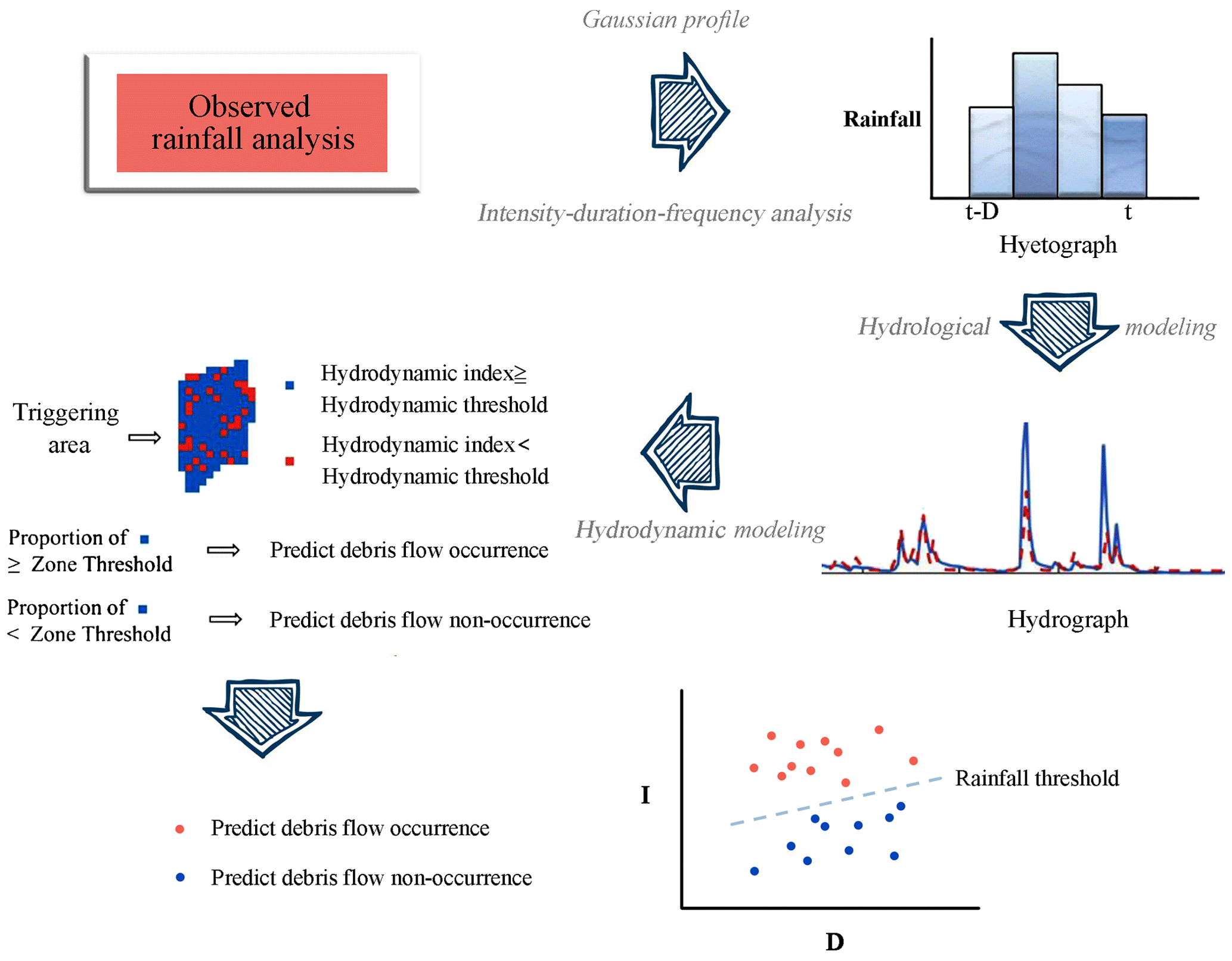
Figure 1 An integrated hydrological and hydrodynamic modeling framework for estimating rainfall thresholds for the occurrence of runoff-generated debris flows.

2.1 Rainfall analysis

IDF analysis plays a pivotal role in generating various synthetic rainfall events for driving hydrological modeling and subsequent analyses within the proposed framework. The IDF curves employed in this study have been derived in accordance with the Atlas of Storms Statistical Parameters for Zhejiang Province, China, the region where our case study is situated (Zhejiang Province Bureau of Hydrology, 2003). This atlas is a comprehensive compilation that draws from rainfall observations from 1953 to 2013 and serves as the authoritative reference for guiding hydraulic engineering design within Zhejiang Province.

Derived from the Pearson Type III probability density function, our IDF curves effectively encompass the range defined by the upper and lower bounds of curves generated by other types of probability functions, such as extreme-value and long-term probability functions. As outlined in the Atlas of Storms Statistical Parameters, it is possible to compute extreme rainfall for various return periods and durations, denoted H_p, as follows:

$$\begin{array}{}\text{(1)}& H_p=K_p\stackrel{\mathrm{‾}}{H},\end{array}$$

where $\stackrel{\mathrm{‾}}{H}$ is the maximum average rainfall of a specific duration and K_p is a coefficient with the subscript p denoting the rainfall duration. The values of both $\stackrel{\mathrm{‾}}{H}$ and K_p can be obtained from the atlas.

Nevertheless, it is important to note that the atlas exclusively provides information on extreme rainfall for durations of 1, 6, and 24 h. Therefore, a method for estimating rainfall with a 3 h duration becomes imperative for the scope of this study. Within the atlas, one can readily compute the rainfall depth (H_i) for rainfall events of duration (t_i) between 1 and 6 h using the following approach:

$$\begin{array}{}\text{(2)}& {\displaystyle }{H}_i=H_{\mathrm{1}\mathrm{h}}{t}_i^{\mathrm{1}-n_{\mathrm{1},\mathrm{6}}},\text{(3)}& {\displaystyle }{n}_{\mathrm{1},\mathrm{6}}=\mathrm{1}+\mathrm{1.285}\lg (H_{\mathrm{1}\mathrm{h}}/H_{\mathrm{6}\mathrm{h}}),\end{array}$$

where H_1 h and H_6 h are the extreme rainfall depths of the 1 and 6 h events, respectively, and n_1,6 is the corresponding attenuation coefficient.

Whilst the IDF analysis only specifies the total rainfall amount (i.e., depth) and duration, a Gaussian profile is further used to distribute the rainfall amount over a specific duration, following the approach used by Tang et al. (2019) and Berti et al. (2020). Compared with other similar studies which suggested the rainfall amount arbitrarily (McGuire and Youberg, 2019; Tang et al., 2019), the design hyetographs generated from IDF analysis may better reflect the actual rainfall characteristics of the study area due to the use of local guidance created from multiple observations.

2.2 Hydrological analysis

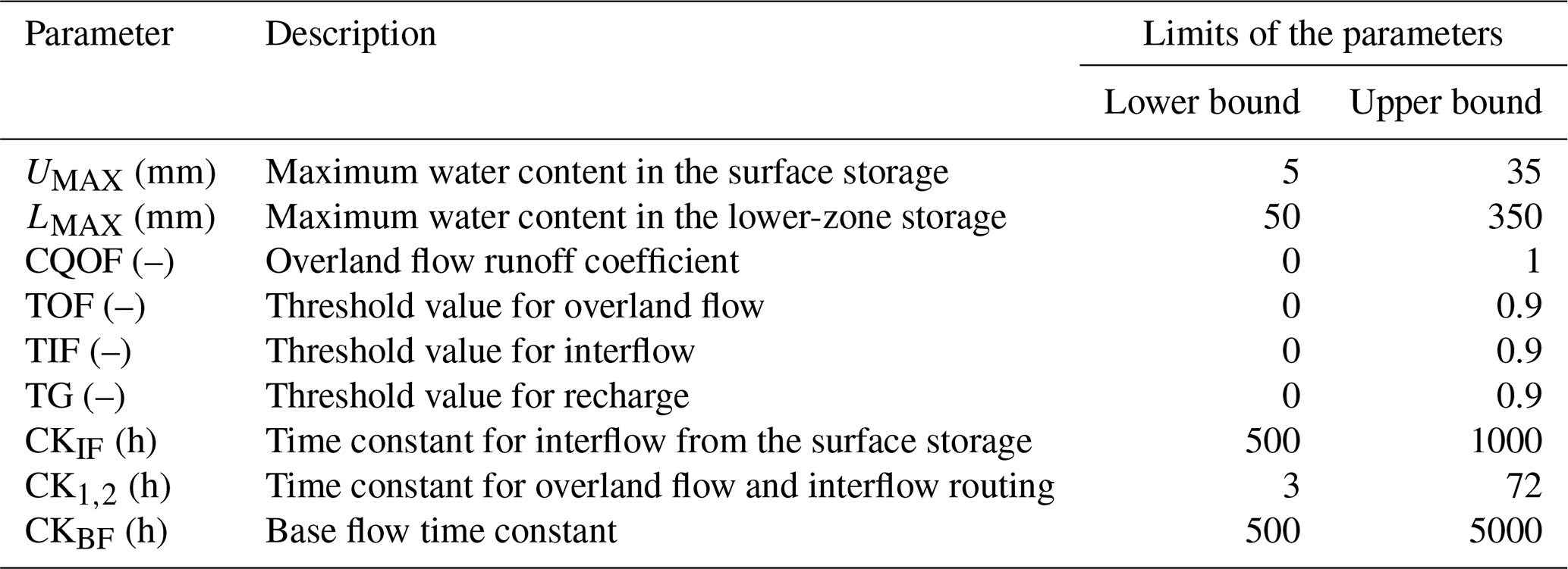
The Nedbør Afstrømnings Model (NAM) (Madsen, 2000) is adopted to simulate the hydrological response to the design rainfall in the headwater catchment of the study site. NAM is part of the MIKE 11 river modeling system (Madsen, 2000), which was developed for simulating rainfall–runoff process in sub-catchments and has been successfully applied in catchments across various climatic regimes including humid areas like the case study site (Butts et al., 2004; Nayak et al., 2013). The structure of the model mainly consists of four mutually interrelated storage components, i.e., snow storage (not used in this work), surface storage, lower-zone (root zone) storage, and groundwater storage, to account for different physical specifications in the precipitation–runoff process (Makungo et al., 2010; Liu and Sun, 2010). The main model inputs are rainfall and temperature (the latter is only needed when snow storage is considered, and it is not relevant in this work).

As NAM is a conceptual model, most of the model parameters are of an empirical or conceptual nature and determined through calibration against hydrological observations. NAM calibration involves the optimization of multiple objectives that consider different aspects of a hydrograph: (1) water balance, (2) the profile of the hydrograph, (3) peak flows, and (4) low flows. An automatic optimization procedure based on the shuffled-complex-evolution algorithm is introduced for solving the multi-objective calibration problem to support model calibration (Madsen, 2000).

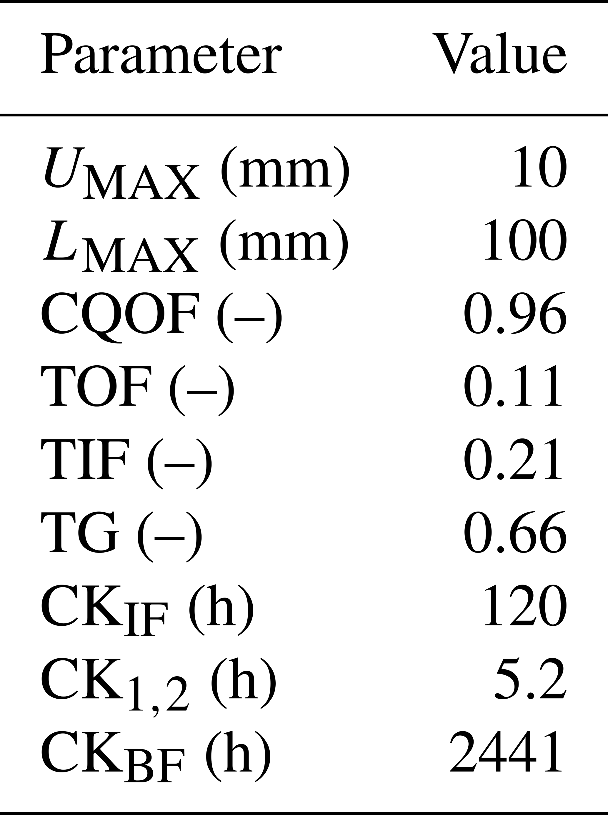
Table 1 lists the nine model parameters used in the simulations conducted in this work, which are linked to the surface zone, the root zone, and the groundwater storage as mentioned.

Table 1 Parameters of NAM involved in this work.

To evaluate the hydrological simulation results, two statistical indices are adopted, i.e., the Nash–Sutcliffe efficiency (NSE) coefficient (Nash and Sutcliffe, 1970) and Schulz criterion (Schulz et al., 1999; Gregoretti et al., 2016). NSE has been widely adopted for evaluating the performance of hydrological models (Nayak et al., 2013; Makungo et al., 2010). The Schulz criterion has been used to validate hydrological simulations in small catchments prone to debris flows, similar to the catchment of the current case study (Gregoretti et al., 2016). The Nash–Sutcliffe coefficient is defined as

$$\begin{array}{}\text{(4)}& \mathrm{NSE}=\mathrm{1}-{\displaystyle \frac{\sum _{i=\mathrm{1}}^N\left[q_{\mathrm{o}}\right(i)-q_{\mathrm{s}}(i){]}^{\mathrm{2}}}{\sum _{i=\mathrm{1}}^N\left[q_{\mathrm{o}}\right(i)-{\stackrel{\mathrm{‾}}{q}}_{\mathrm{o}}{]}^{\mathrm{2}}}},\end{array}$$

where i is the data index, N is the total number of data points, q_o is the observed discharge (m³ s⁻¹), q_s is the simulated discharge (m³ s⁻¹), and ${\stackrel{\mathrm{‾}}{q}}_{\mathrm{o}}$ is the average of the observed discharge (m³ s⁻¹).

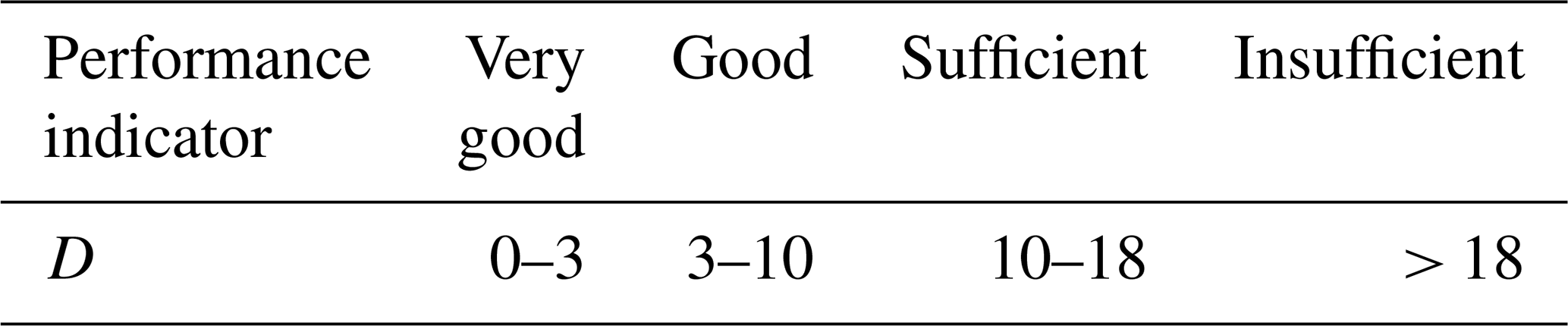
The Schulz criterion is a model performance indicator defined as follows:

$$\begin{array}{}\text{(5)}& D=\mathrm{200}{\displaystyle \frac{\sum _{i=\mathrm{1}}^N\left|q_{\mathrm{s}}\left(i\right)-q_{\mathrm{o}}\left(i\right)\right|q_{\mathrm{o}}\left(i\right)}{N{\left(q_{\mathrm{o},\max }\right)}^{\mathrm{2}}}},\end{array}$$

where q_o,max is the observed maximum discharge (m³ s⁻¹). The Schulz criterion classifies the performance of a hydrological model into four categories, ranging from very good to insufficient, as listed in Table 2.

Table 2 Model performance classified by the Schulz criterion (Schulz et al., 1999).

2.3 Hydrodynamic modeling

In the proposed modeling framework, the High-Performance Integrated hydrodynamic Modelling System (HiPIMS) (Xia et al., 2019) is employed to predict the grid-based flow information (i.e., water depth and velocity/discharge) in the debris-flow-triggering area, driven by the output hydrograph(s) from hydrological modeling/analysis in the considered headwater catchment. HiPIMS solves the following fully 2D shallow-water equations (SWEs):

$$\begin{array}{}\text{(6)}& {\displaystyle \frac{\partial \mathit{q}}{\partial t}}+{\displaystyle \frac{\partial \mathit{f}}{\partial x}}+{\displaystyle \frac{\partial \mathit{g}}{\partial y}}={\mathit{S}}_b+{\mathit{S}}_{\mathrm{f}},\end{array}$$

where t is the time; q is the vector containing the flow variables; f and g are the flux vectors in the x and y directions; and S_b and S_f are the source term vectors representing the bed slope and friction effect, respectively. The vector terms are given by

$$\begin{array}{}\text{(7)}& {\displaystyle }\mathit{q}=\left[\begin{array}{l}h\\ uh\\ vh\end{array}\right],\mathit{f}=\left[\begin{array}{l}uh\\ u^{\mathrm{2}}h+\frac{\mathrm{1}}{\mathrm{2}}g{h}^{\mathrm{2}}\\ uvh\end{array}\right],\mathit{g}=\left[\begin{array}{l}vh\\ uvh\\ v^{\mathrm{2}}h+\frac{\mathrm{1}}{\mathrm{2}}g{h}^{\mathrm{2}}\end{array}\right],\text{(8)}& {\displaystyle }{\mathit{S}}_b=\left[\begin{array}{l}\mathrm{0}\\ -gh\frac{\partial b}{\partial x}\\ -gh\frac{\partial b}{\partial y}\end{array}\right],{\mathit{S}}_{\mathrm{f}}=\left[\begin{array}{l}\mathrm{0}\\ -\frac{{\mathit{\tau }}_{bx}}{\mathit{\rho }}\\ -\frac{{\mathit{\tau }}_{by}}{\mathit{\rho }}\end{array}\right],\end{array}$$

where h is the water depth, u and v are the two depth-averaged velocity components in the x and y directions, ρ is the water density, g is the gravitational acceleration, and τ_bx and τ_by are the frictional stresses estimated using the Manning equation:

$$\begin{array}{}\text{(9)}& {\mathit{\tau }}_{bx}=\mathit{\rho }{C}_{\mathrm{f}}u\sqrt{u^{\mathrm{2}}+v^{\mathrm{2}}},{\mathit{\tau }}_{by}=\mathit{\rho }{C}_{\mathrm{f}}v\sqrt{u^{\mathrm{2}}+v^{\mathrm{2}}}.\end{array}$$

Here C_f is the roughness coefficient calculated using

$$\begin{array}{}\text{(10)}& C_{\mathrm{f}}=g{n}^{\mathrm{2}}/h^{\mathrm{1}/\mathrm{3}},\end{array}$$

where n is the Manning coefficient.

HiPIMS solves the above governing equations using a Godunov-type finite-volume numerical scheme, making it suitable for simulating different types of shallow-flow hydrodynamics, including the high-transience flash flooding processes induced by dam breaks or intense rainfall. HiPIMS is also implemented in multiple graphics processing units (GPUs) to achieve high-performance computing and has been intensively tested for modeling catchment-scale overland flow and flooding processes as well as other types of flood hydrodynamics (Ming et al., 2022; Chen et al., 2022). HiPIMS is therefore suited for predicting the transient and complex flow hydrodynamics across different flow regimes in the debris-flow-triggering area, as required by this work. More details of the model can be found in Xia et al. (2019) and Ming et al. (2020).

2.4 Hydrodynamic indices and thresholds

Previous studies have demonstrated that the transition from runoff to a debris-dominated flow may occur when the surface-water flow exceeds the thresholds of critical flow discharge (Gregoretti and Dalla Fontana, 2008; Gregoretti, 2000; Recking, 2009). Different formulae have been reported to estimate the critical discharge that triggers a runoff-generated debris flow. In this study, the equations proposed by Wang et al. (2017) and Whittaker et al. (1989) are considered. The formula introduced by Wang et al. (2017) calculates the critical unit-width discharge (q_c) as

$$\begin{array}{}\text{(11)}& q_{\mathrm{c}}=\mathrm{0.32}{\displaystyle \frac{d_{\mathrm{84}}^{\mathrm{2.5}}}{(\tan \mathit{\theta }{)}^{\mathrm{2}}{d}_{\mathrm{16}}{C}_u{C}_c^{\mathrm{0.4}}}},\end{array}$$

where θ is the mean gradient angle of the triggering area; d₈₄ and d₁₆ are the 84 % and 16 % grain diameters in the particle size distribution curve; and $C_u=d_{\mathrm{60}}/d_{\mathrm{10}}$ and C_c= ($d_{\mathrm{30}}{)}^{\mathrm{2}}/(d_{\mathrm{60}}{d}_{\mathrm{10}}$) are the non-uniformity and curvature coefficients, with d₆₀, d₃₀, and d₁₀ denoting the 60 %, 30 %, and 10 % grain diameters, respectively. Equation (11) explicitly takes into account the inhomogeneity of sediment and has been shown to provide a reliable estimation of critical discharge (Wang et al., 2017). Most previous formulae are based on the mean grain diameter by assuming homogeneous or narrowly graded sands and therefore do not consider the effect of inhomogeneity of gully bed materials on debris-flow initiation, which may potentially lead to less accurate results. Specifically relevant to the current study, the mean slope of the triggering area under consideration is within the range investigated by Wang et al. (2017).

The equation reported by Whittaker et al. (1989) was developed to calculate the critical discharge that leads to the destabilization of artificial block ramps (hydraulic structures built with boulders to stabilize riverbeds) and is written as

$$\begin{array}{}\text{(12)}& q_{\mathrm{c}}=\mathrm{0.257}(s-\mathrm{1}{)}^{\mathrm{0.5}}{g}^{\mathrm{0.5}}{d}_{\mathrm{65}}^{\mathrm{1.5}}(\tan \mathit{\theta }{)}^{-\mathrm{1.17}},\end{array}$$

where s is the ratio of the sediment density (ρ_s) to water density (ρ) and d₆₅ is the 65 % grain diameter in the particle size distribution curve. As Eq. (12) was proposed to evaluate the erosion of block ramps with large blocks, it is used in this work to calculate the critical discharge that initiates the motion of large boulders in the triggering area.

In the implementation, the grid-based water depths and flow velocities predicted by HiPIMS are used to calculate the corresponding unit-width discharge q (m² s⁻¹) in each grid cell in the triggering area as

$$\begin{array}{}\text{(13)}& q=h\sqrt{u^{\mathrm{2}}+v^{\mathrm{2}}},\end{array}$$

which is then used to define the hydrodynamic index in each grid cell and is compared with the hydrodynamic thresholds (i.e., critical unit-width discharge) calculated using Eqs. (11) and (12) to indicate the potential occurrence of debris flows.

3 Case study

The proposed framework is applied to estimate the rainfall thresholds for triggering runoff-generated debris flows in a small catchment in Zhejiang Province, China.

3.1 Description of the study site

The study catchment is located in Fenghua, Zhejiang Province, China. As shown in Fig. 2, the catchment has an area of about 0.17 km² and is crossed by a provincial road (No. 33 Provincial Road) constructed in 2013. Downstream of the catchment, a countryside road connects the village of Lingjiao to the outside. The area is dominated by a subtropical monsoon climate, with most of the precipitation occurring in the summer months (1000–1700 mm annual rainfall). In particular, the study catchment often suffers from typhoons that may bring in extreme rainfall and cause flooding and other hydro-geohazards, e.g., debris flows. For example, the excessive rainfall associated with Typhoon Fitow triggered a debris flow on 5 October 2013. The deposit fan of debris flow blocked the aforementioned countryside road, severely interrupting people's livelihoods. The increased risk of debris flows in the catchment is attributed to the availability of loose debris material deposited in channels (triggering area). The loose material was produced during the construction of No. 33 Provincial Road and can be easily eroded and transform into debris flows once the necessary hydrodynamic conditions are met.

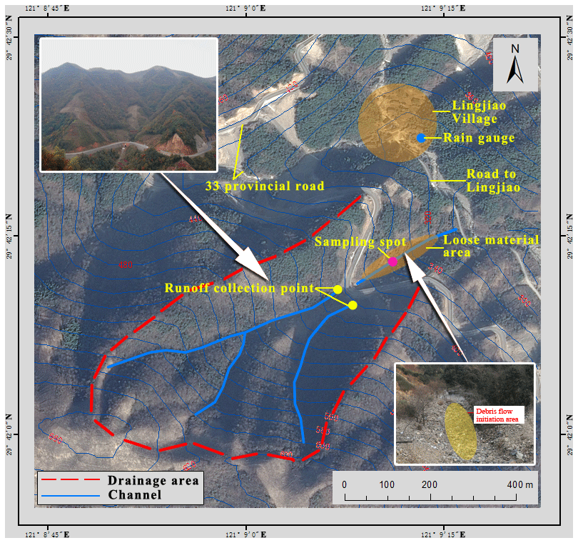
Figure 2 The study area and locations of monitoring instruments (modified from Wei et al., 2018).

As illustrated in Fig. 2, the study catchment is divided into two parts by the provincial road: south of the road is the headwater catchment area, and north of the road is the triggering area where the loose construction wastes are distributed. In Fig. 2, the top-left inset provides an aerial view of the study area, offering a comprehensive overview of the geographic context. The bottom-right inset specifically focuses on the debris-flow initiation area, providing a close-up view to highlight its key features and characteristics. When a large rainfall event hits the headwater catchment area, the induced overland flow will converge into the main channel. Through the culvert underneath the road, the flow will travel into the triggering area and erode the loose soil materials to create a large volume of water and sediment mixture, subsequently forming a debris flow. Table 3 summarizes the morphological characteristics of the catchment, extracted from the ASTER Global Digital Elevation Model (ASTER GDEM) of 5×5 m spatial resolution (Wei et al., 2018).

Table 3 Morphological characteristics of the catchment (A_c is the catchment area (km²); θ_TRIG is the average slope of the triggering area; Y_out is the altitude at the outlet; Y_org is the altitude at the channel head).

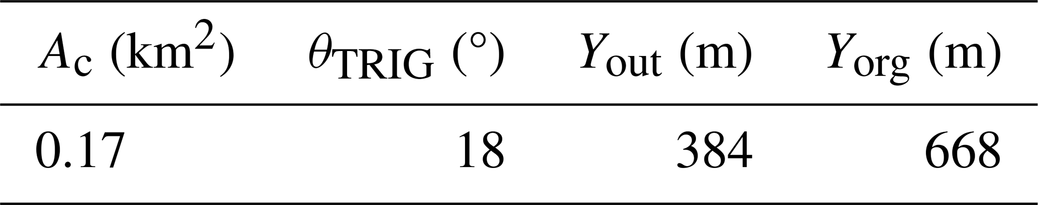
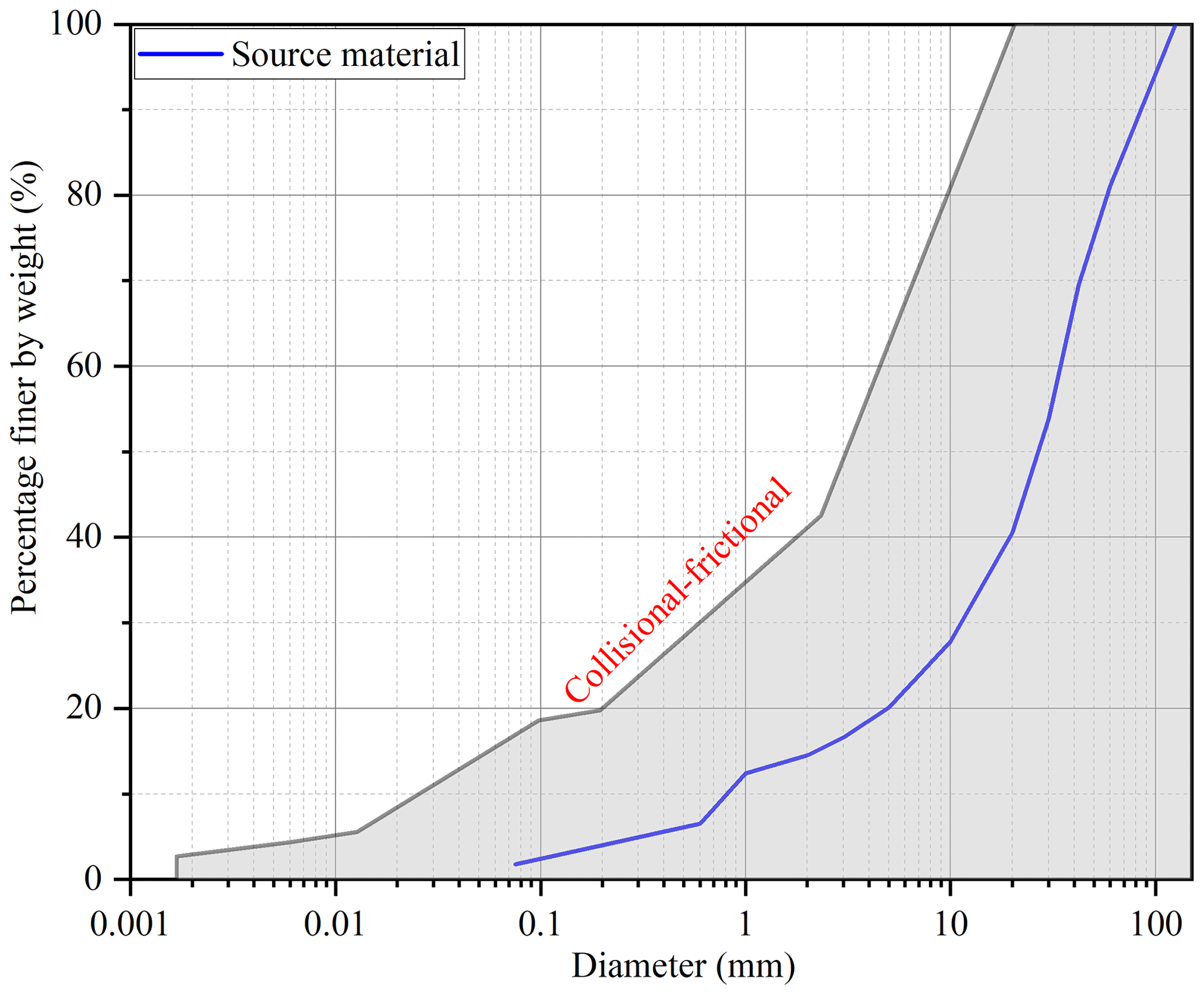
Figure 3 Grain-size distribution derived from the soil sample collected in the triggering area; the rheological class proposed by Bardou et al. (2003) is added as a reference.

Grain-size distribution (GSD) has been demonstrated to be an effective index to characterize the rheological behavior of debris flows. Herein, we adopt a simple sieving method to obtain the GSD of the loose material. An approx. 0.1 m³ soil sample is taken from a 2 m × 1 m rectangular window at the site. The maximum grain size is analyzed to be about 120 mm, whilst the minimum grain diameter is approx. 0.075 mm (Fig. 3). Bardou et al. (2003) classified debris flows into two main rheo-physical types, i.e., the viscoplastic class including the muddy debris flows that demonstrate a Herschel–Bulkley or Bingham flow behavior and the collisional class of stony debris flows that are featured with a Coulomb-like flow behavior. As shown in Fig. 3, the study area may be characterized as a collisional regime, most likely forming stony debris flows.

3.2 Monitoring system

A monitoring system was set up to record rainfall and flow discharge in the case study site. For rainfall monitoring, a HOBO RG3-M tipping-bucket rain gauge produced by Onset, USA, was installed. The rain gauge has a resolution of 0.2 mm per tip, meaning that the device will generate records for cumulative rainfall greater than 0.2 mm. Debris flows are usually triggered by locally convective rainfall that covers only a small storm cell (a few square kilometers or even less). It is therefore important to install a rain gauge that is as close as possible to the triggering zone to ensure the reliability of rainfall records (Simoni et al., 2020). In this case, the rain gauge was installed on the roof of a house in the village of Lingjiao (Fig. 2), which is only about 200 m away from the study site and means misrepresenting rainfall conditions can effectively be avoided.

To measure flow discharge, two triangular weirs were installed at the outlets of the two channels from the headwater catchment, just in front of the culvert (Fig. 4). The flow discharge is derived from a rating curve based on the measured water level. The rating curve used in this study is computed by solving the continuity equation recommended by Berti et al. (2020). To minimize water surface oscillations that may affect the reliability of water-level measurement during extreme flow conditions, two approximately rectangular stilling basins (about 1.2 m wide and 2.0 m long) were also constructed on the upstream sides of the weirs. The bottoms of the stilling basins were flattened and built with concrete. The water level was measured using a pressure–water-level recorder (Odyssey Capacitance water-level logger) installed inside a vertical PVC pipe; the recorder has a resolution of approximately 0.8 mm. The PVC pipe was installed in each of the stilling basins to improve stability, i.e., avoiding vibration of the PVC pipes caused by the water flow. In addition, holes were created along the vertical direction to synchronize the changing water level with the ambient flow (Wei et al., 2018). The data logger sampled the water-level records at a 10 min interval. The weirs were thin-walled with a 90° notch. The monitoring system operated successfully for about 1 month, during which six rainfall events occurred, which provides short but reliable high-quality measurements to support the current study.

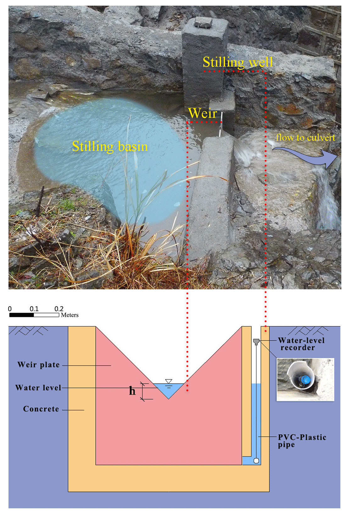
Figure 4 Water discharge measuring system (modified from Wei et al., 2018).

The outflow discharge (Q_W) from the head catchment is estimated based on the continuity equation:

$$\begin{array}{}\text{(14)}& Q_W\left(t\right)={\displaystyle \frac{\mathrm{d}{V}_{\mathrm{b}}}{\mathrm{d}t}}+Q_{\mathrm{b}},\end{array}$$

where V_b is the volume of water in the stilling basin, which is a function of the water depth. d$V_{\mathrm{b}}/\mathrm{d}t$ can be approximated using the backward finite-difference method:

$$\begin{array}{}\text{(15)}& \begin{array}{rl}{\displaystyle \frac{\mathrm{d}{V}_b}{\mathrm{d}t}}\approx {\displaystyle \frac{\mathrm{\Delta }{V}_{\mathrm{b}}}{\mathrm{\Delta }t}}& ={\displaystyle \frac{V_{\mathrm{b}}\left(i\right)-V_{\mathrm{b}}(i-\mathrm{1})}{\mathrm{10}\times \mathrm{60}}}\\ & ={\displaystyle \frac{A_{\mathrm{b}}{h}_b\left(i\right)-A_{\mathrm{b}}{h}_b(i-\mathrm{1})}{\mathrm{10}\times \mathrm{60}}},\end{array}\end{array}$$

where h_b is the water depth recorded at a 10 min interval, i indexes the time step, $\mathrm{\Delta }t=\mathrm{10}\times \mathrm{60}$ (s), and A_b= 2.4 m² is the area of the stilling basin. Q_b (m³ s⁻¹) is the discharge over the weir calculated using the formula recommended by the Water Supply and Drainage Design Manual of China (Southwest Institute of Municipal Engineering Design and Research, 2000):

$$\begin{array}{}\text{(16)}& Q_{\mathrm{b}}=\mathrm{1.343}(h/\mathrm{1000}{)}^{\mathrm{2.47}}.\end{array}$$

The formula is applicable for thin-walled weirs with a weir angle of 90°, and the water depth over the weir falls within the range of 0.02 to 0.35 m. The discharge calculated using this equation should range from $\mathrm{8.9}\times {\mathrm{10}}^{-\mathrm{5}}$ to 0.1 m³ s⁻¹.

4 Results

In this section, the predicted flow discharge is first compared with the observation data to calibrate and verify the hydrological model. Then, rainfall events with and without triggering a debris flow are considered to validate the proposed modeling methodology. Finally, driven by the design rainfall events generated from IDF analysis, the proposed framework is applied to predict the rainfall thresholds for triggering debris flows. For hydrological modeling, the time interval of the input rainfall data is 1 h and the temporary resolution of the predicted hydrographs is 10 min. The hydrodynamic modeling results are recorded every 10 min to maintain consistency with the hydrological modeling outputs.

4.1 Hydrological simulation results

The effective discharge measurements are considered herein to evaluate the hydrological model introduced in Sect. 2.2, which covers six rainfall events over 1 month, as shown in Fig. 5. The monitoring period is divided into two parts, i.e., from 3 to 15 July and from 26 July to 3 August, for model calibration and verification, respectively. It is important to note that no debris flow occurred during the depicted rainfall events, and all the observed discharge represented in Fig. 5 corresponds to clear water flow.

Figure 5 Recorded rainfall, observed discharge, and simulated discharge at the study site.

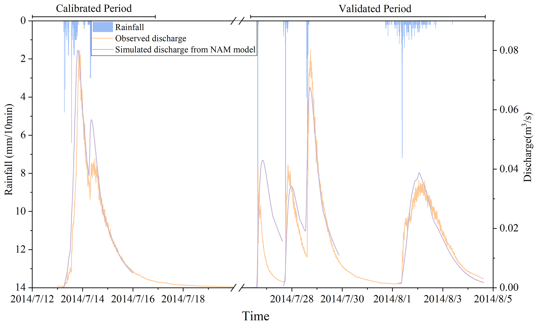
NAM is first calibrated automatically to decide the initial parameters, using an automatic calibration scheme as introduced in Sect. 2.2. Subsequently, a trial-and-error method is further used to refine parameter values by visually comparing the simulated and observed hydrographs. Hydrological simulations in the study area have already been conducted by Wei et al. (2018) using part of the hydrological monitoring data and are enriched in this study using more monitoring data to further validate the hydrological model. The final values of the model parameters are listed in Table 4. Figure 5 compares the predicted discharge amounts with the observed data during the calibration process. The predicted flow discharges agree reasonably well with the observations. The model predicts a peak discharge at 0.081 m³ s⁻¹, which is close to the observed peak of 0.079 m³ s⁻¹. Quantitatively, the Nash–Sutcliffe efficiency (NSE) and Schulz criterion (D) calculated from the NAM predictions are presented in Table 5. The rainfall events on 13 and 14 July of the calibration period and also the ones on 27 and 28 July of the validation period are jointly assessed as they occurred close to each other and can reasonably be regarded as “continuous” events. NAM returns 0.89 and 4.64 for NSE and D, respectively. According to the Schulz criterion, the performance of NAM is ranked “good”.

Table 4 Calibrated model parameters for NAM.

Table 5 The statistical matrices calculated from model calibration and verification.

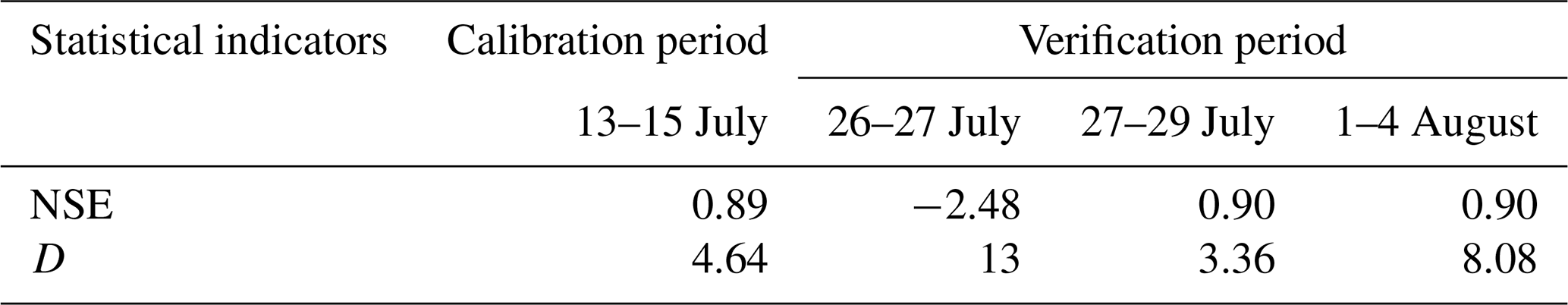
The calibrated version of NAM is then applied to reproduce the second part of the 1-month measured data for model verification. The discharge hydrograph predicted for 26 to 27 July does not compare well with the measurements, as reflected by the low value returned for NSE and high value for the Schulz criterion; i.e., NSE = −2.48 and D= 13. The poor performance of the model for this specific event may be because the model is not specifically calibrated for short-duration and high-intensity storms like the one under consideration (36 mm in 25 min). During the calibration period, the rainfall intensity was relatively low, and the runoff was mainly generated as a result of insufficient catchment storage following a sufficiently long rainfall event. However, for the event during 26–27 July, the intensity of the rainfall was excessive and may have been significantly greater than the catchment infiltration rate, subsequently generating excess infiltration runoff. Even so, NAM estimates the peak discharge to a reasonable level of accuracy, i.e., 0.041 m³ s⁻¹ against the observed value of 0.043 m³ s⁻¹, and the relative error is only 5 %.

From the results as shown in Fig. 5, it can be seen that NAM performs better for the rest of the verification period and satisfactorily reproduces the observed hydrographs, which is confirmed by the returned values of the statistical indicators; i.e., NSE = 0.90 and D = 3.3 and NSE = 0.90 and D= 8.1. Following model verification, it is found that NAM can effectively reflect the rainfall–runoff process at the study site and can be used in the following simulations and analysis.

Close examination of the numerical results can find that NAM may slightly overestimate or underestimate flood peaks in both the calibration and the validation periods. The relative errors calculated against the observed and simulated peak discharge amounts for the six rainfall events are 1.2 %, 25 %, 5 %, 17 %, 14 %, and 6 %, respectively. Sensitivity analysis has previously been conducted by Wei et al. (2018) to identify the key parameters influencing peak discharge calculation. The results revealed that CQOF, U_max, and CK₁₂ exhibited a more profound influence on peak discharge calculation. Whilst the sensitivity analysis provided valuable insights, further research may still be needed in the future to investigate and confirm the performance of the model in reproducing catchment response to different rainfall patterns when more measured data become available.

To further test the capability of the calibrated NAM in simulating the hydrological response to short-duration and high-intensity rainfall like the 26–27 July rainstorm, an experiment is conducted to re-calibrate the model to the event. A comparison between observed and simulated discharge hydrographs for the event is shown in Fig. 6. It should be noted that only the 26–27 July rainstorm was used for the calibration process. It is clear that NAM performs better during the re-calibration process and satisfactorily reproduces the observed hydrographs, which is confirmed by the returned statistical indicators; i.e., NSE = 0.59 and D= 10.4. The model parameters obtained after re-calibration are listed in Table 6. To further support model evaluation, the Kling–Gupta efficiency (KGE) index is also considered for the re-calibration process (Kling et al., 2012), with a returned value of 0.56 providing an additional assessment and confirmation of model performance.

Figure 6 Comparison between observed and simulated hydrographs for the 26–27 July storm.

Table 6 The re-calibrated parameter values for NAM.

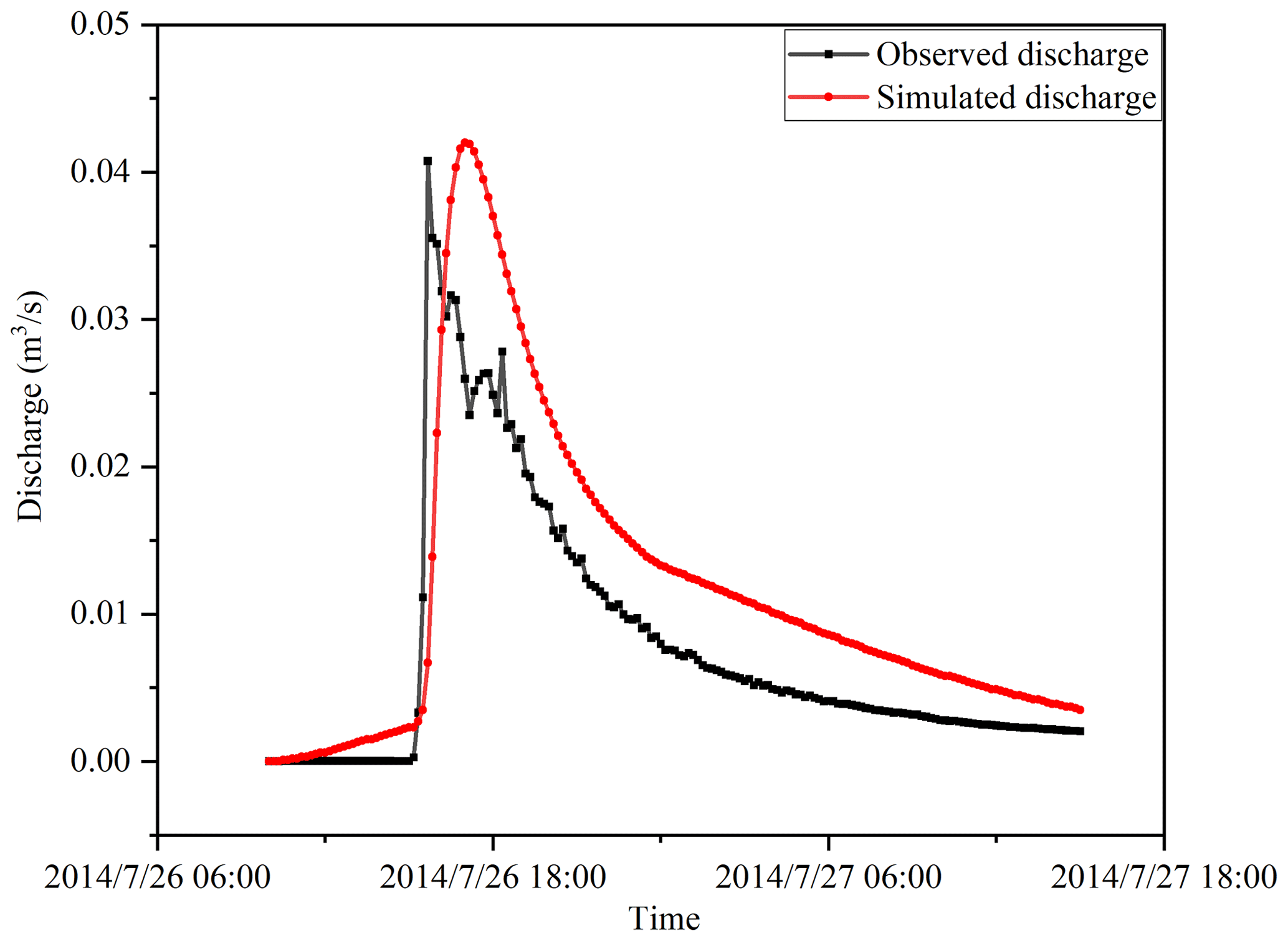
From Table 6, it can be found that only the values of CK_1F and CK_1,2 changed significantly, whilst the other model parameters did not experience much change during re-calibration. The calibrated values of CK_1F and CK_1,2 changed from 754 and 11.3 to 125 and 5, respectively, at the re-calibration. CK_IF and CK_1,2 are time constants related to the routing of overland flow and may have a significant impact on the lag time between the timing of peak discharge and rainfall. They should therefore be carefully calibrated and checked for cases of short-duration and high-intensity storms. According to Simoni et al. (2020), a rainfall burst or short-duration and high-intensity rainfall event occurs if the rainfall intensity reaches or exceeds 0.2 mm per 5 min (i.e., burst intensity threshold). Following this definition, a rainfall event with a duration shorter than 1 h and an intensity greater than 25 mm h⁻¹ may be classified as a short-duration, high-intensity rainfall event, e.g., the 26–27 July event considered in this work. The reproduction of the 26–27 July event indicates that the selected model is capable of simulating the hydrological responses to different hyetographs including short-duration, high-intensity rainfall events. Even though the occurrence frequency of short-duration and high-intensity events is rare in the study area (see Supplement, Figs. S1 and S2), the proposed framework may be used to estimate the initiation of runoff-generated debris flows under a wide range of rainfall conditions, including rainstorms leading to infiltration excess overland flows and events causing saturation excess overland flows.

4.2 Validation of the proposed framework

In this section, the proposed methodology framework is tested for predicting a runoff-generated debris flow. As described in Eq. (6), the initiation of runoff-generated debris flows is primarily influenced by the grain-size distribution and the slope of the channel. In this study, the initiation area is relatively small, so we did not take into account the spatial variations in the grain-size distribution. Instead, we treated the grain-size distribution as constant throughout the area. The channel slope also plays a role in the initiation of debris flows. We analyzed the statistical features of the slope in the triggering area, using a digital elevation model (DEM) with a resolution of approximately 5 m × 5 m. The results indicated that the standard deviation of the slope was only about 3.2°. Therefore, we assumed that the slope could be adequately represented by its mean value, and we considered the hydrodynamic threshold to be spatially constant. Based on the grain-size distribution and the topography characteristics of the study area, the critical discharge calculated from Eq. (11) is 0.024 m² s⁻¹, which is defined as the hydrodynamic threshold G. To calculate the critical discharge mobilizing larger blocks, we follow a similar process to that reported by Pastorello et al. (2020). The grain size is chosen to be 100 mm (i.e., d₆₅= 100 mm as the representative size for boulders) as the maximum grain size in the triggering area is about 125 mm. Then, based on Eq. (12), the critical discharge for mobilizing sparse boulders is calculated to be 0.12 m² s⁻¹, which is defined as the hydrodynamic threshold W.

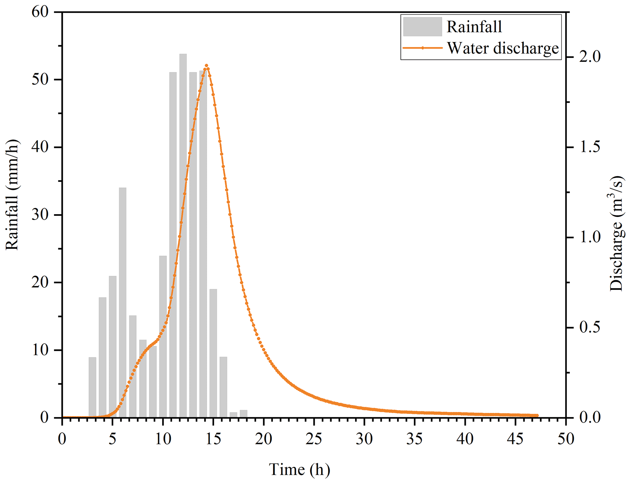
In October 2013, a debris flow occurred in the case study site, triggered by the intense rainfall brought in by Typhoon Fitow. Unfortunately, no monitoring instrumentation was installed in the study area at the time; i.e., the catchment was ungauged. Therefore, the rainfall data from the nearest station (Huangtuling; 10 km away) are used. The total rainfall amount of the October 2013 rainfall event was 380 mm with the rainfall duration being 16 h. The characteristics of the rainfall event were analyzed by Wang et al. (2015), who showed that the heavy rainfall was more than 300 mm and covered an area of about 258 km² (including the current study area). The rainfall records from the Huangtuling station are considered to be relevant and are used to drive NAM to predict the hydrograph out of the upper catchment, as shown in Fig. 7.

Figure 7 The rainfall input and predicted hydrograph during Typhoon Fitow in the study area.

The predicted hydrograph is then used to drive HiPIMS to predict grid-based hydrodynamic information (i.e., water depth and flow velocity) in the triggering area, discretized using a DEM of 5 m spatial resolution. A uniform Manning coefficient of 0.04 is used to reflect the vegetation cover of the study area as suggested by Arcement and Verne (1989). The input hydrograph is applied at a particular input point/cell located at the outlet of the culvert beneath the road as the point-source boundary conditions to drive HiPIMS to simulate the subsequent flow dynamics. During an intense rainfall event that occurred in the headwater catchment area, the generated overland flow converges into the main channel, passes through the culvert beneath the road, reaches the triggering area, and erodes the available loose soil materials to initiate a debris flow. From the output simulation results in terms of water depth and velocity, the unit-width discharges are calculated for each grid cell, across the entire simulation domain. Figure 8 presents the distribution of the unit-width discharge from each cell in the triggering area at the time when the peak flow is reached, along with the threshold values.

Figure 8 Distribution of unit-width discharge amounts along with the threshold values.

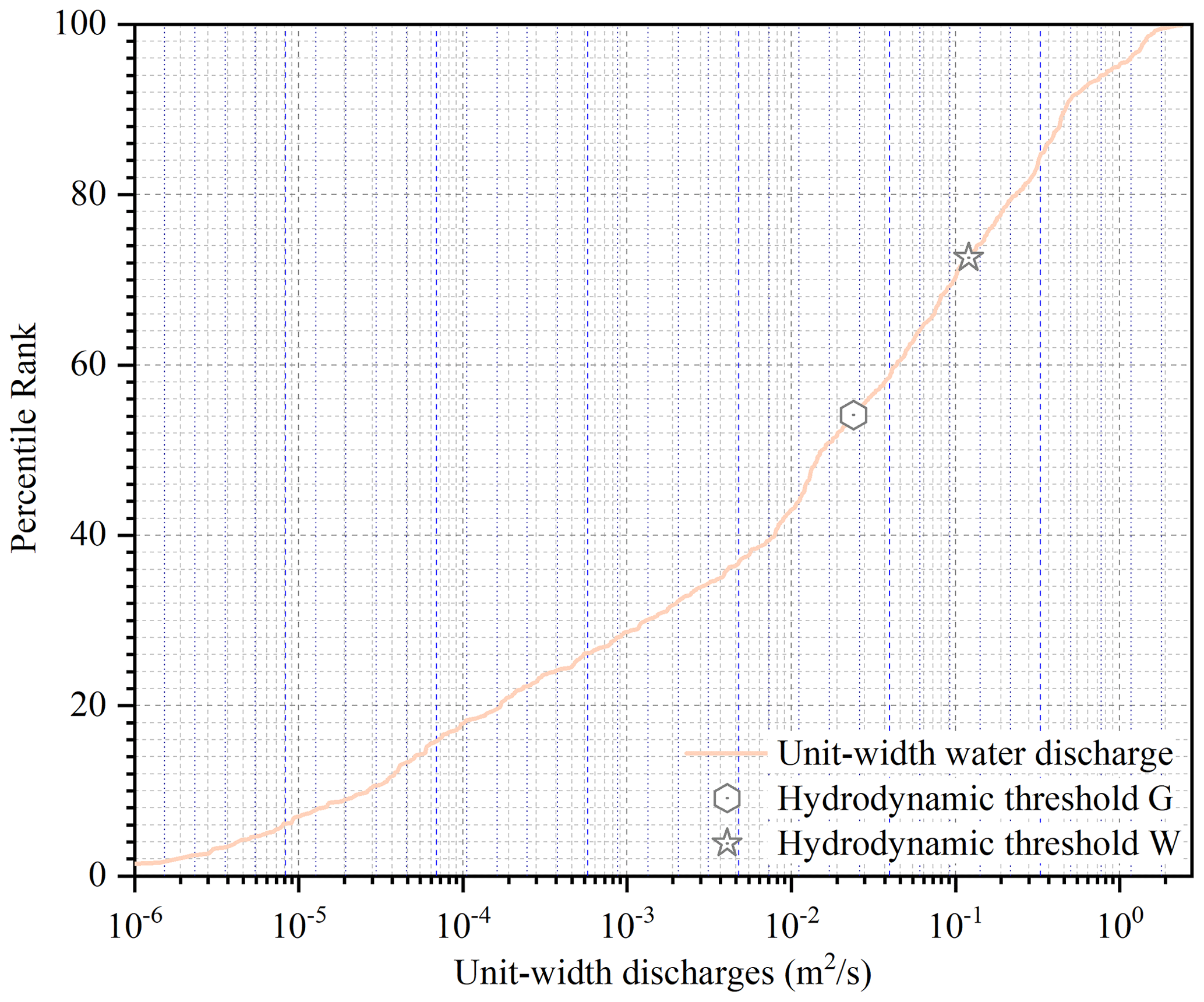
From Fig. 8, it can be seen that the unit-width discharge ranges from 0 to 2.42 m² s⁻¹ across the triggering area. From the discharge distribution curve, the corresponding percentiles reaching the hydrodynamic thresholds G and W are 54 % and 72 %, respectively. This essentially means that 46 % and 28 % of the grid cells in the computational domain (i.e., triggering area) are predicted with a unit-width discharge larger than the hydrodynamic thresholds G and W. That is also to say that the hydrodynamic conditions for a runoff-generated debris flow have been met in areas covered by 46 % of the grid cells according to the hydrodynamic threshold G. Even based on the much higher threshold W, 28 % of the grid cells have been predicted with the required hydrodynamic conditions. Therefore, considerably large areas (at least 28 %) are estimated to reach the required conditions that can trigger a debris flow. The results are consistent with the actual observation – i.e., a debris flow did occur during the typhoon event – demonstrating that the proposed methodology successfully predicted the occurrence of this debris-flow event.

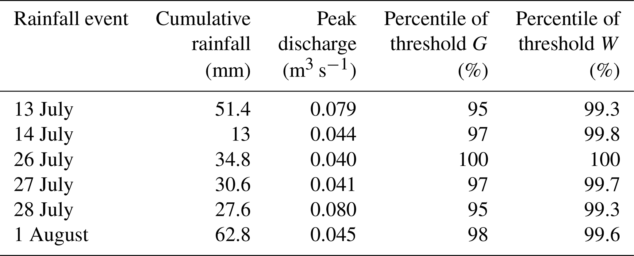
We also consider the six rainfall events that did not trigger a debris flow to further test and confirm the predictability of the proposed framework. Figure 9 shows the unit-width discharges predicted in each grid cell for the six events, along with the threshold values. The distributions of the unit-width discharges between the 13 and 28 July events are very similar because the rainfall peaks are almost the same. Table 7 further lists the relevant hydrological information. Among the six non-triggering rainfall events, it is observed that the lowest percentiles for the unit-width discharge reaching the hydrodynamic thresholds G and W are 95 % and 99.3 %, respectively, indicating that only 5 % and 0.7 % of the grid cells inside the triggering area are predicted to reach or exceed the hydrodynamic thresholds of G and W. This implies that the hydrodynamic conditions necessary for triggering a debris flow are met in only a small fraction of the grid cells and that the likelihood of debris-flow occurrence is very low. This conclusion aligns with the actual observations; i.e., no debris flow was observed during these six rainfall events. As a whole, these numerical tests demonstrate the capability of the framework including the adopted hydrodynamic thresholds in predicting six observed non-debris-flow events and one actual debris-flow event.

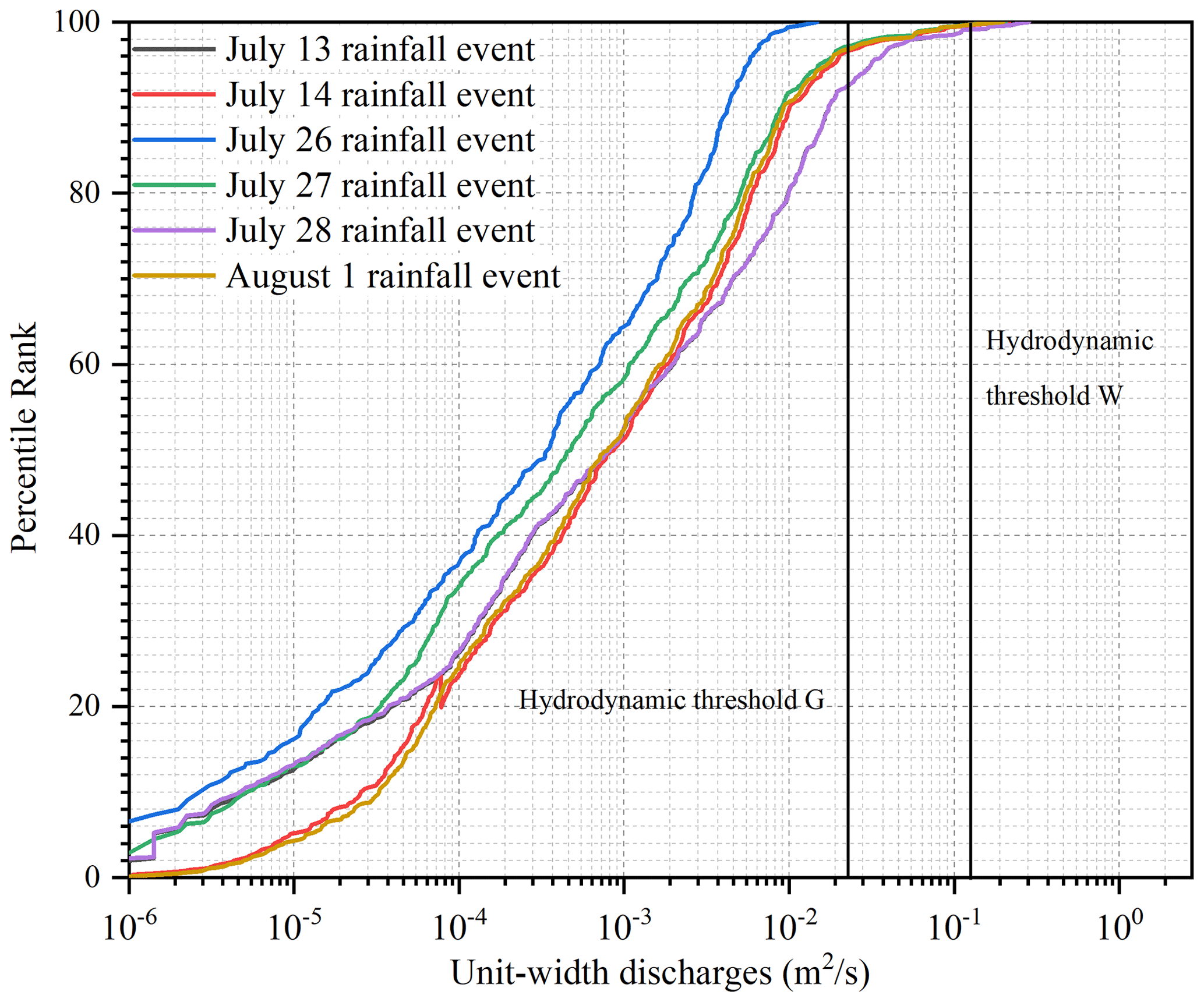
Figure 9 Distribution of unit-width discharges along with the threshold values predicted for the six rainfall events that did not trigger a debris flow.

Table 7 Hydrological information on the six rainfall events that did not trigger a debris flow.

To further demonstrate the feasibility of the threshold framework, we have also conducted several extra-scenario simulations. Specifically, we modified the input rainfall events, varying the cumulative amount from 10 % to 110 % of the original rainfall that triggered the 2013 debris flow. The rainfall distribution is presented in Fig. 10. The cumulative input rainfall ranges from 38 to 418 mm, with the original value that triggered the 2013 debris flow being 380 mm. The calculated discharge for each scenario is shown in Fig. 11. Additionally, the calculated peak discharge and the corresponding proportion of triggering cells based on the G threshold are detailed in Table 8.

Figure 10 Rainfall distribution of the extra-scenario simulations.

Figure 11 Calculated runoff of the extra-scenario simulations.

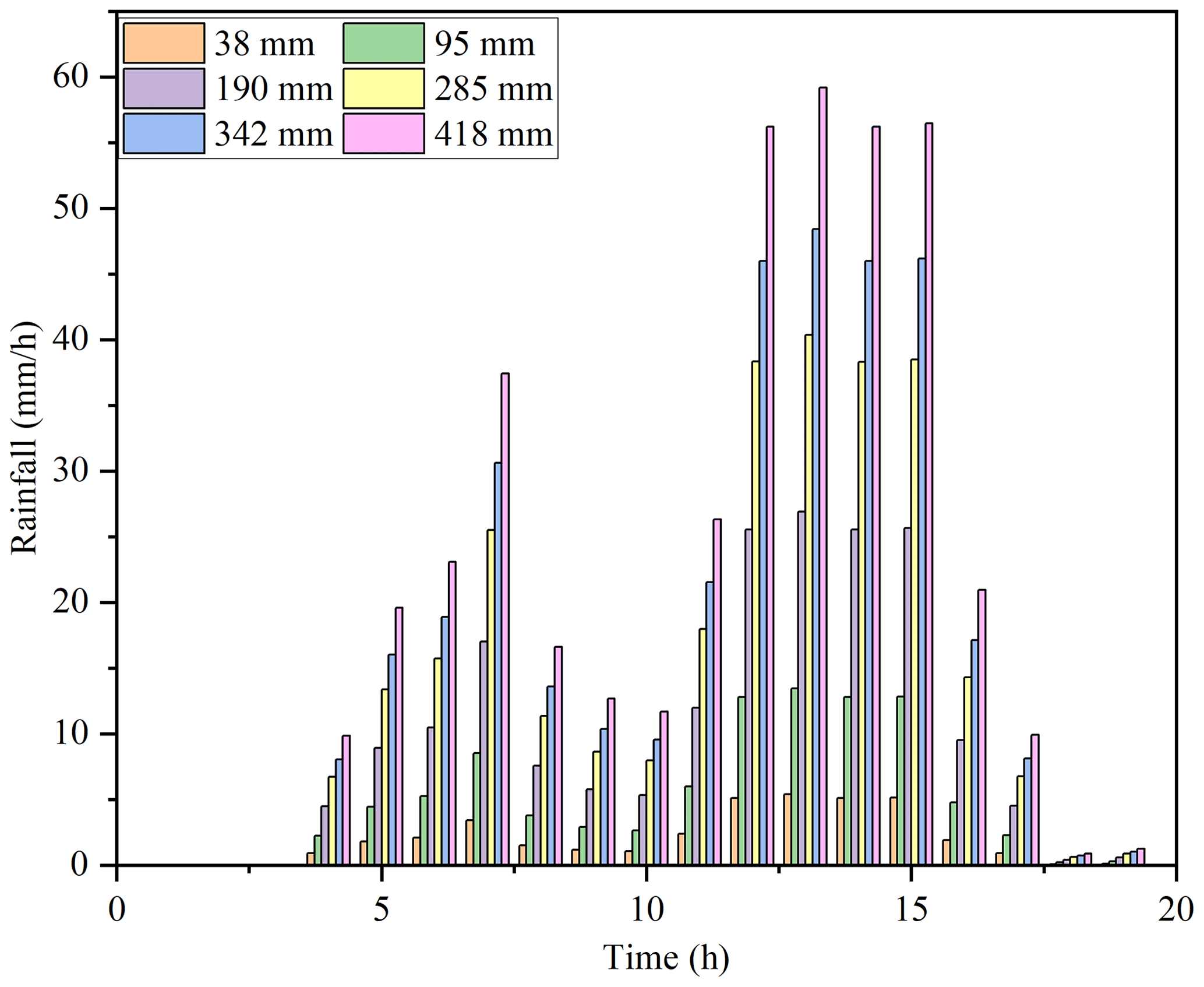
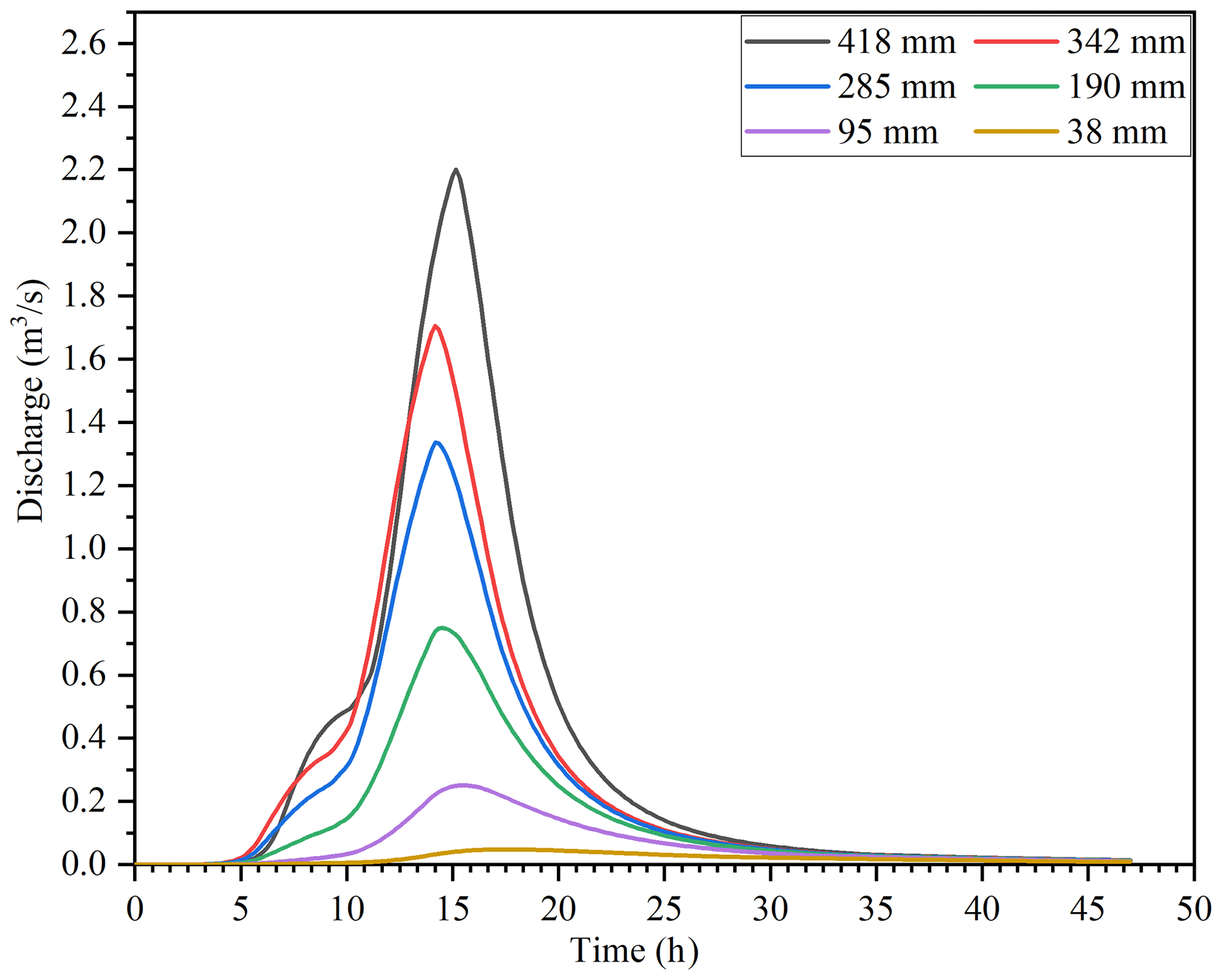
Table 8 The calculated peak discharge and the corresponding proportion of triggering cells.

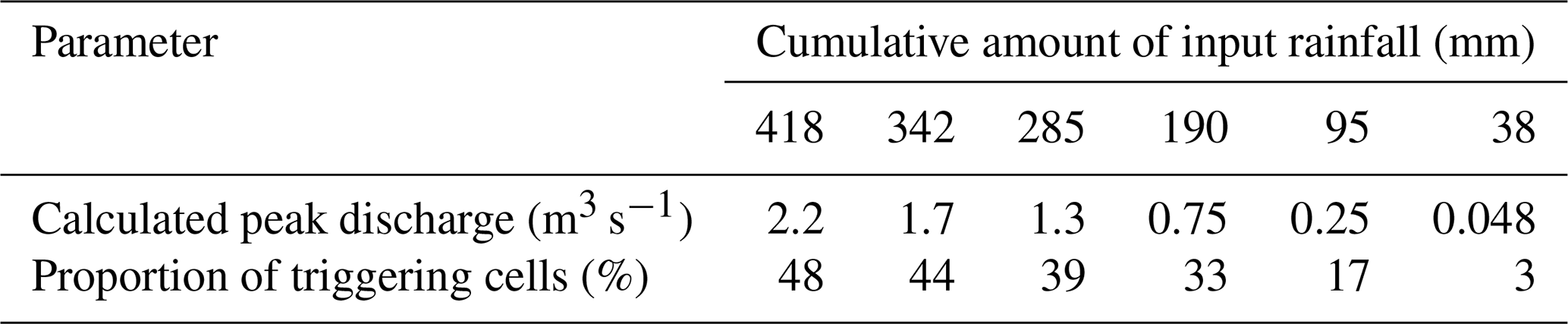
The calculated peak discharge from the rainfall that triggered the 2013 debris flow is 2.0 m³ s⁻¹. As shown in Table 8, rainfall events resulting in discharge amounts greater than the one in 2013 could also result in debris-flow events, with the calculated proportion of triggering cells for the 418 mm rainfall event being 48 %. Even discharge slightly lower than the 2013 event may still trigger a debris flow, as indicated by the 342 mm rainfall event, which has a calculated triggering cell proportion of 44 %. The numerical experiment demonstrates that the calculated proportion of triggering cells is consistent with the change in the input rainfall.

4.3 Estimation of rainfall thresholds using the proposed framework

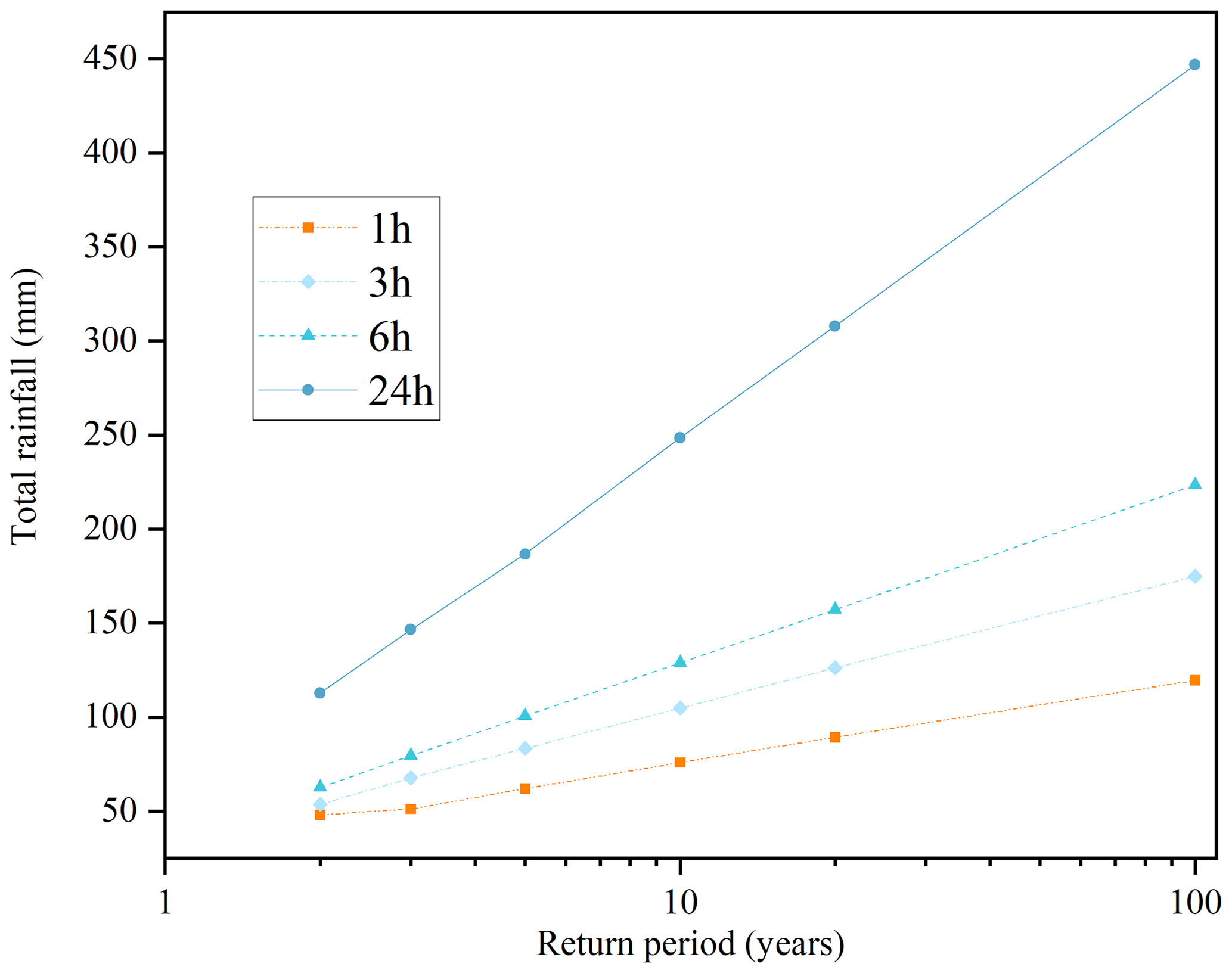
Design rainfall of different return periods and durations is obtained for the study area through IDF analysis. In this study, we consider rainfall with a return period of 100, 20, 10, 5, 3, and 2 years and a duration of 1, 3, 6, and 24 h. Therefore, a total of 24 design rainfall events are generated, as illustrated in Fig. 12.

Figure 12 The design rainfall events obtained through IDF analysis.

The 24 design rainfall events are then input into NAM to predict the corresponding flow hydrographs from the headwater catchment, which are shown in Fig. 13. The resulting rainfall profiles have different times to peak for design events of different rainfall durations. For example, the times to peak for the 3 h rainfall and 6h rainfall are 120 and 240 min, respectively. From the results, it can be seen that a shorter rainfall duration, e.g., 1 or 3 h, leads to lower flow discharge relative to an event with a longer duration (e.g., 6 or 24 h). This is consistent with other studies in the literature. For example, Pastorello et al. (2020) reported a similar conclusion and suggested that longer rainfall duration is needed to generate flow discharge large enough to mobilize large blocks.

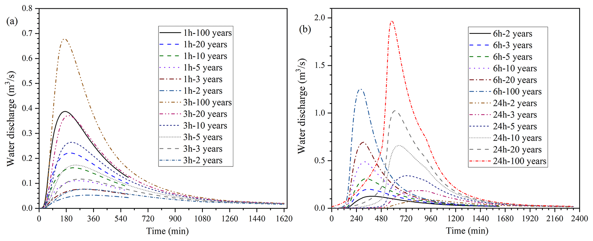
Figure 13 Predicted hydrographs for different design rainfall events: (a) 1 and 3 h events and (b) 6 and 24 h events. In the legends, the return period and duration of rainfall events are given; for example, “1 h–100 years” means the rainfall event of a 100-year return period and 1 h duration.

The predicted hydrographs are then used as the inputs for HiPIMS to predict the corresponding grid-based flow information for calculating unit-width discharge. Figure 14 shows the distributions of unit-width discharge for different design rainfall events along with the relevant hydrodynamic thresholds. The results may then be analyzed to indicate the likely occurrence of a debris flow.

The objective of this study is to calculate ID rainfall thresholds to classify rainfall events into two categories: trigger events and non-trigger events. Rather than predicting the occurrence of debris flows in each grid cell, the focus is on determining whether a given rainfall event will potentially trigger debris flows at the catchment scale. To achieve this, it is necessary to establish a criterion based on a critical proportion of trigger cells in the triggering area to determine whether a specific rainfall event can be classified as a trigger event for the entire catchment. Following the approach reported by Zhao et al. (2020), such a critical proportion is defined as the zone threshold for the triggering area, which can then be integrated with the hydrodynamic thresholds to estimate a rainfall threshold.

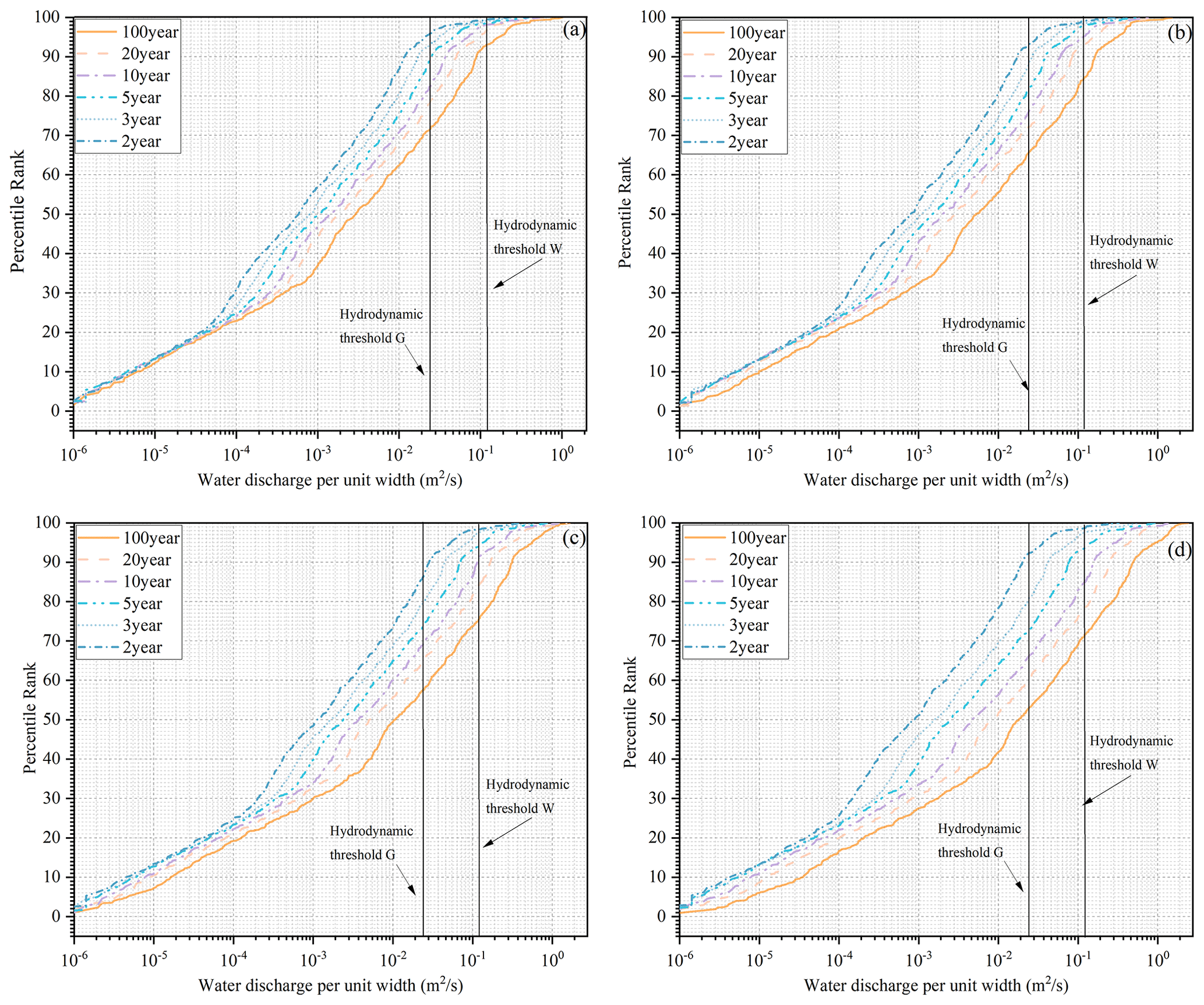
Figure 14 Distributions of unit-width discharge when the peak flow discharge occurs, along with corresponding Hydrodynamic thresholds: (a) 1 h rainfall events, (b) 3 h rainfall events, (c) 6 h rainfall events, and (d) 24 h rainfall events.

To define the zone threshold, the calculated grid-based unit-width discharges are compared with the hydrodynamic thresholds G and W. If any of the thresholds are exceeded, the associated grid cell is registered as a trigger cell. If the proportion of trigger cells in the triggering area exceeds a critical value, i.e., zone threshold, a debris flow is considered to be triggered; otherwise, it will be considered a non-occurrence event (Fig. 1). In this study, 5 % of the grid cells are used to define the non-triggering rainfall condition whilst 46 % are used to define the triggering rainfall condition. Six different zone thresholds (i.e., 5 %, 10 %, 15 %, 20 %, 25 %, and 30 %) are tested to investigate their influence on the results. A trigger rainfall event is identified if a zone threshold is exceeded (as presented in Fig. 14). In this way, the rainfall thresholds associated with different zone thresholds can be decided, which are shown in Fig. 15. The rainfall conditions of the Typhoon Fitow event, which has a return period of about 100 years, are also included in Fig. 15.

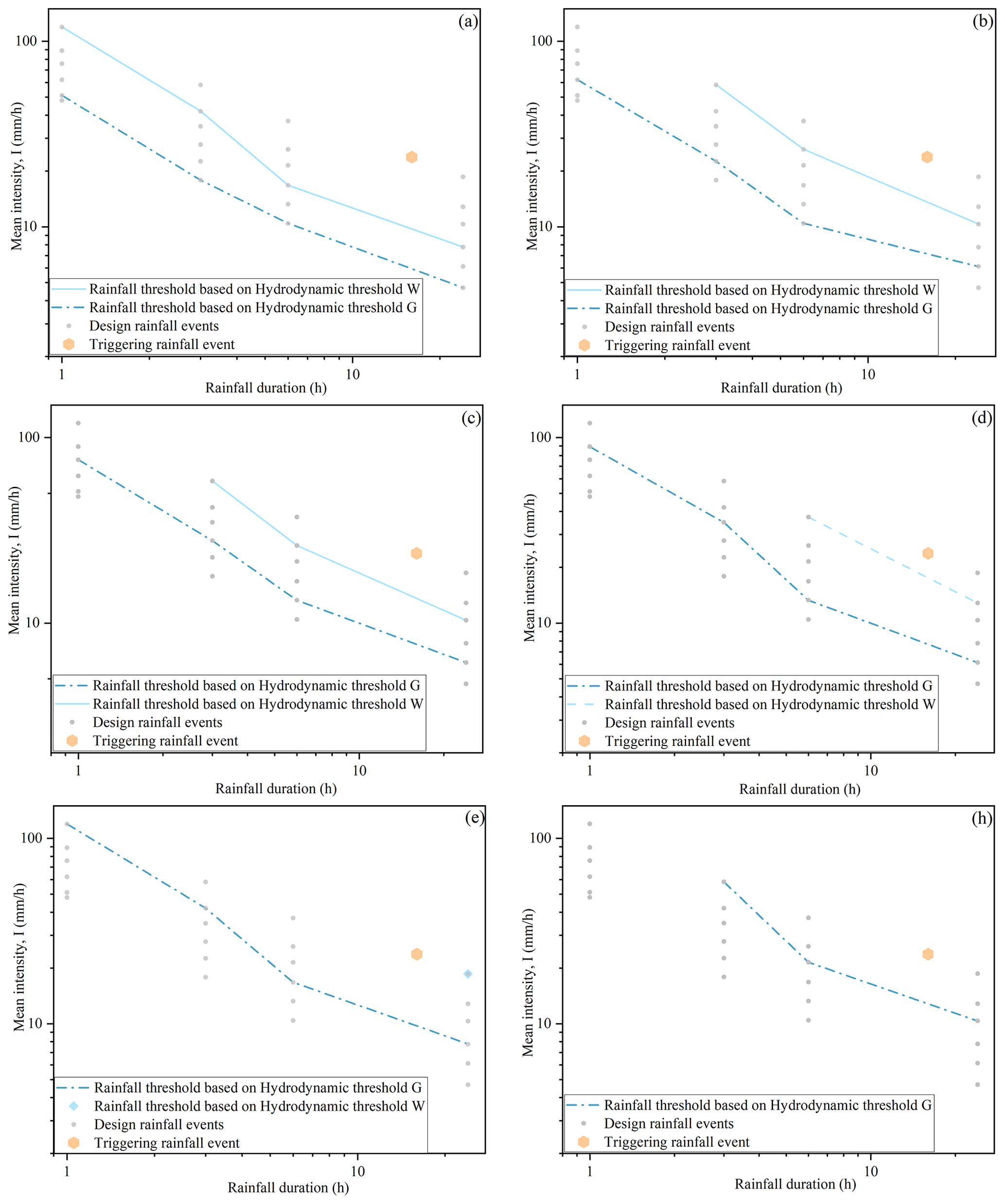
Figure 15 Rainfall thresholds associated with different zone thresholds: (a) 5 %, (b) 10 %, (c) 15 %, (d) 20 %, (e) 25 %, and (h) 30 %.

From Fig. 15, the calculated rainfall thresholds show an increasing trend as the zone threshold increases. This is as expected because a larger amount of rainfall is needed to generate more triggering cells. In addition, the rainfall conditions of Typhoon Fitow are beyond both the rainfall threshold based on threshold G and that based on threshold W considering different zone thresholds. This means the proposed rainfall threshold is reasonable. The chosen values of the zone threshold can also represent different levels of conservatism or adventurousness in the generated rainfall thresholds.

Comparing the two adopted hydrodynamic thresholds, the rainfall thresholds calculated based on W are normally larger, whilst those calculated based on G are smaller. The initiating mechanism to derive the hydrodynamic threshold G assumes that progressive scouring occurs in sediment layers, which requires a lower critical discharge and subsequently a smaller amount of rainfall. The hydrodynamic threshold W is built on the assumption of full bed failure, which needs a larger hydrodynamic force and more rainfall to trigger the failure. The intervals between the two corresponding rainfall thresholds are also related to the dynamics of a debris flow. At the beginning of a rainfall event, the resulting flow discharge is small, which increases as the rainfall amount and duration increase. When the discharge reaches the hydrodynamic threshold G, the first surge of debris flow may form although the volume is usually small. If the rainfall continues to intensify, the hydrodynamic conditions evolve. When the maximum discharge exceeds the hydrodynamic threshold W, bed failure may occur, which will lead to a sudden increase in the debris-flow volume. Mobilization of large blocks may worsen the situation and lead to the generation of the peak of the debris flow in terms of both flow and sediment volumes. Capra et al. (2018) investigated the temporal sequence of debris flows by comparing monitoring data (including video images, seismic records, and rainfall data) with the numerically predicted hydrological response of the watershed under consideration. It was shown that the pulses of a debris-flow event are not randomly distributed in time and that the largest pulse is most commonly connected with the peak discharge.

Specifically, in Fig. 15d, it can be seen that only three sets of design rainfall (24 h–100 years, 24 h–20 years, and 6 h–100 years) may trigger a debris flow associated with the hydrodynamic threshold W. When the zone threshold is taken to be 25%, only one design rainfall event (24 h–100 years) can potentially trigger a debris flow. In Fig. 15h, no design rainfall under consideration can trigger a debris flow again if the calculation is based on the hydrodynamic threshold W.

Herein, we also compare the proposed intensity–duration (ID) rainfall thresholds with the regional rainfall ID statistical thresholds. Figure 16 presents a comparison between the proposed rainfall thresholds obtained with a zone threshold of 10 % and the empirical ID thresholds. The regional empirical rainfall thresholds were obtained after analyzing the main characteristics (duration and intensity) of rainfall events that had triggered 1569 landslides (including many runoff-generated debris flows events) in Zhejiang Province during the period between 1990 and 2013 (Ma et al., 2015). Ma et al. (2015) also estimated the ID thresholds of 62 mountainous counties or cities in Zhejiang Province, including the city Fenghua in which the study area is located. It should be noted that the ID threshold from Ma et al. (2015) is the only rainfall threshold developed in the study area. From Fig. 16, it is evident that both the proposed ID rainfall threshold and the empirical rainfall threshold can effectively distinguish between one triggering rainfall event and six non-triggering rainfall events, highlighting the feasibility of the proposed framework. In addition, the present rainfall thresholds are located above the empirical thresholds when the rainfall duration is short (e.g., 1 and 3 h). But as rainfall duration increases, the empirical rainfall thresholds cross all three curves of the proposed rainfall thresholds, and then they are located below the empirical thresholds. Using the proposed thresholds as references, the results indicate that the empirical thresholds may underestimate the occurrence of debris flows for short-duration rainfall events and overestimate the occurrence for longer-duration rainfall.

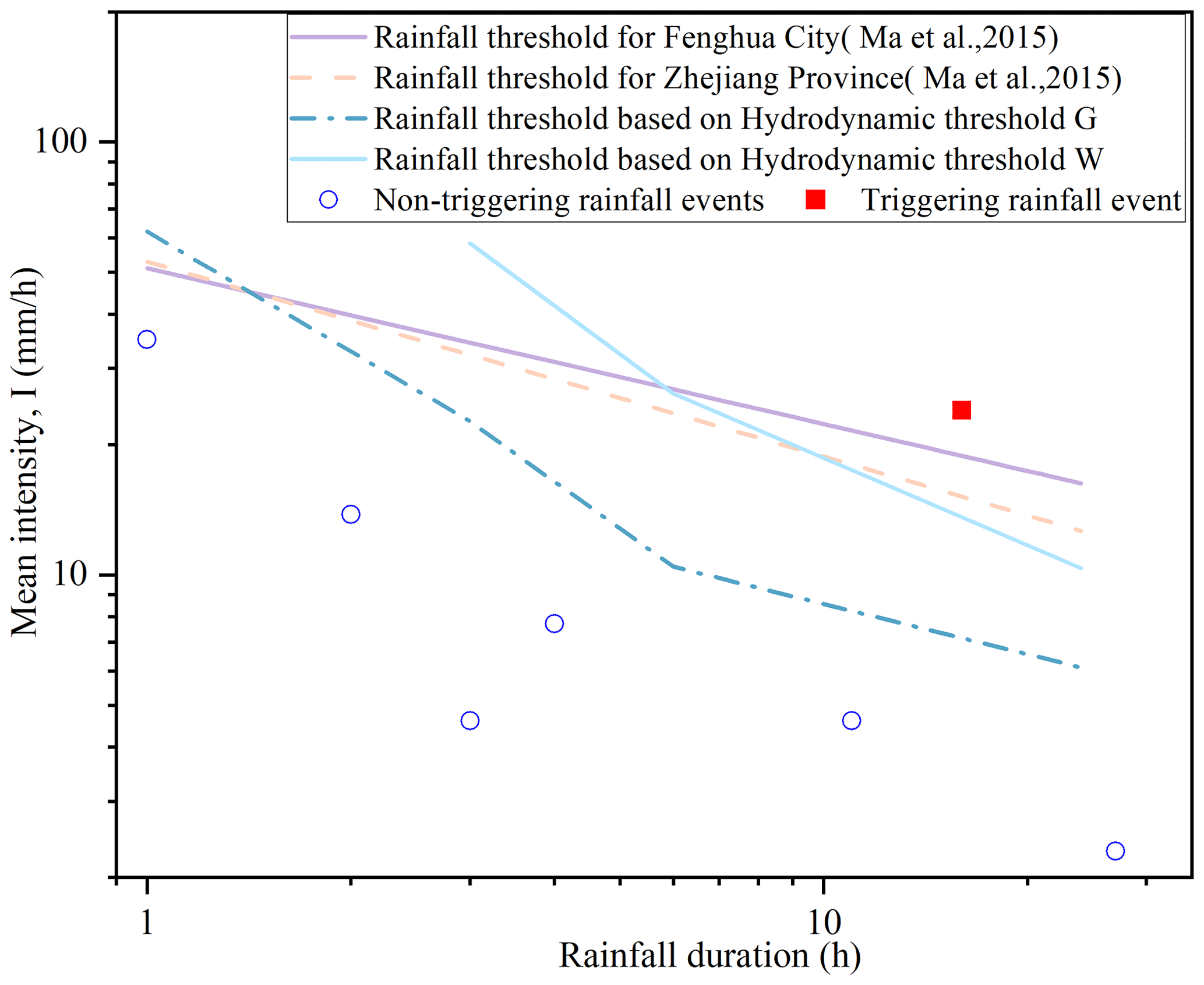
Figure 16 Comparison between present rainfall thresholds and the regional empirical ID thresholds.

5 Discussion

Model assumptions and physical processes in the targeted catchment will have a direct effect on the final estimation of rainfall thresholds. For example, the grain size of sediment may increase as surface flow washes away the fine particles. Such progressive coarsening of the debris-flow material is called “grain coarsening”. Field observations have suggested that such a process can be quick and that fine soil may be washed away over just a few years (Domènech et al., 2019). To evaluate potential uncertainties, the values of physical thresholds are changed from 50 % to 200 % with an increment of 10 %, creating a total of 16 physical thresholds. The estimated rainfall thresholds corresponding to the different zone thresholds are shown in Figs. 17 and 18. For the hydrodynamic threshold G, the values of the critical threshold (CR) change from 0.012 to 0.048 m² s⁻¹, whilst for the hydrodynamic threshold W, the CR varies from 0.06 to 0.24 m² s⁻¹.

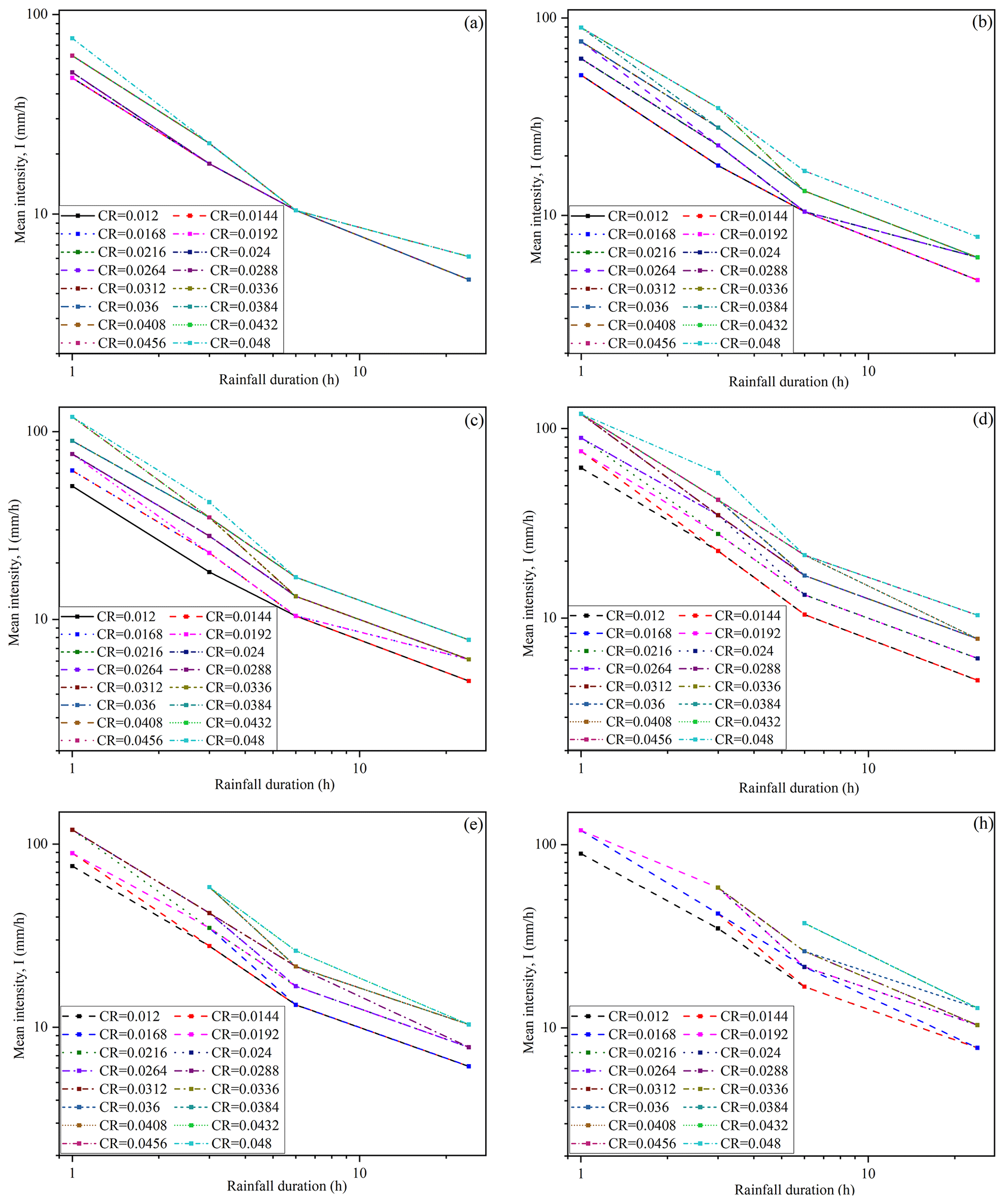
Figure 17 Sensitivity analysis of rainfall thresholds based on the hydrodynamic threshold G associated with different zone thresholds: (a) 5 %, (b) 10 %, (c) 15 %, (d) 20 %, (e) 25 %, and (h) 30 %.

From Fig. 17, it is clear that the variation range of rainfall intensity is narrow when the zone threshold is small. When the zone threshold is 5 %, the rainfall intensity only increases from 48 to 79 mm h⁻¹ for a 1 h event; when the rainfall duration is 6 h, there is not much change in the rainfall intensity even when the physical threshold changes significantly. Therefore, the rainfall intensity is not sensitive to the variation in the physical threshold when the zone threshold is small, indicating that it is not suitable to set the zone threshold to be overly small (like 5 %). The variation range of rainfall intensity widens when the zone threshold increases. When the zone threshold is set to 20 %, the rainfall intensity increases from 62 to 112 mm h⁻¹ for a 1 h event and the change becomes even greater for events with longer rainfall durations, e.g., 3, 6, and 24 h. This indicates that rainfall intensity is sensitive to the change in physical thresholds when the zone threshold is sufficiently large.

Figure 18 shows the variation in the rainfall intensity following the change in the hydrodynamic threshold W. Compared with the results related to the hydrodynamic threshold G as shown in Fig. 17, the rainfall intensity is found to vary in a wider range even when the zone threshold is small (Fig. 18a). When further increasing the zone threshold, fewer rainfall events can trigger debris flows. When the zone threshold reaches 30 % (Fig. 18h), no rainfall event can induce debris flows when the critical threshold is assumed to be larger than 0.096 m² s⁻¹.

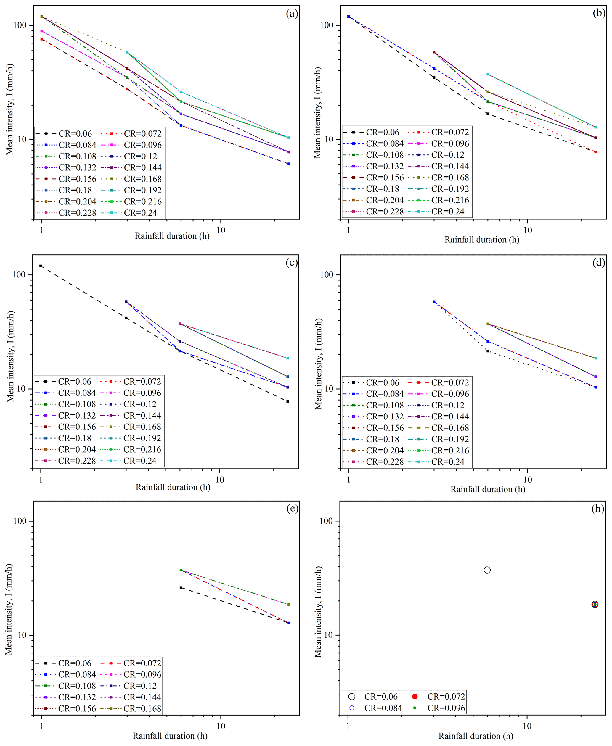
Figure 18 Sensitivity analysis of rainfall thresholds based on hydrodynamic threshold W associated with different zone thresholds: (a) 5 %, (b) 10 %, (c) 15 %, (d) 20 %, (e) 25 %, and (h) 30 %.

The importance of hydrological and hydrodynamic processes in triggering runoff-generated debris flows has been recognized and discussed. Due to the scarcity of observed flow data but better availability of rainfall data, the statistical ID rainfall thresholds are still mostly used, although their development does not consider the hydrological process and flow hydrodynamics. However, the reliability of statistical ID rainfall thresholds depends on the data being used, and therefore high-quality long-term observations are essential to derive reliable thresholds. This indicates that a statistical approach may be difficult to reliably apply in ungauged catchments where high-quality historical data are missing.

In this work, a new approach is explored to predict the potential occurrence of runoff-generated debris flows by integrating hydrological and hydrodynamic models to predict rainfall-induced hydrological response and the resulting surface flow hydrodynamics. Compared with the traditional statistical ID analysis approaches that only consider meteorological factors, the proposed modeling framework can effectively take into account the meteorological conditions, topographic properties of the targeted catchment, and grain-size distribution of debris materials. The use of a fully physically based hydrodynamic model enables the proposed framework to generate rainfall thresholds in areas with limited historical data on debris-flow occurrence. As the hydrodynamic thresholds (e.g., critical discharge) should not vary with the hydrological properties of the catchments, the framework can be readily applied to other similar catchments (e.g., alpine regions) when essential data are available for model calibration and setup.

To date, several studies have been reported to establish intensity–duration (ID) rainfall thresholds through a numerical approach (Domènech et al., 2019). In the previous studies, runoff-induced erosion is considered to occur when the bed shear stress exceeds a critical value and the volumetric concentration of solids in the debris flow is smaller than an equilibrium value. Furthermore, most of the previous studies adopt simplified hydrological simulations, e.g., calculating runoff using a basic lumped infiltration model that neglects the initial moisture content of the soil. In contrast to these existing attempts, the proposed approach focuses on predicting a spatially varying hydrodynamic index (unit-width discharge) in each cell to indicate the occurrence of runoff-generated debris flows.

In the authors' previous works (Wei et al., 2018, 2017), the rainfall thresholds at the same study site were also calculated using a runoff prediction model. Wei et al. (2018) developed an approach solely based on a hydrological model, whilst Wei et al. (2017) presented a machine learning model for runoff prediction. These approaches are different from the current integrated hydrological and hydrodynamic modeling framework, which provides a more robust method to directly incorporate overland flow dynamics into debris-flow occurrence estimation. Furthermore, our previous studies used peak discharge as the critical parameter to indicate debris-flow occurrence; if the peak discharge predicted by the adopted hydrological model exceeds the critical discharge, debris-flow occurrence is confirmed. Whilst such peak-discharge-based approaches can estimate debris-flow occurrence, they cannot provide any insights related to the magnitude and scale of a debris flow. Our new framework includes the use of a hydrodynamic model to predict detailed overland flow dynamics and derive grid-based hydrodynamic indices in the areas susceptible to debris flows. This not only enables the prediction of debris-flow occurrences but also provides insights into the magnitude and scale of a debris flow.

Furthermore, to evaluate debris-flow occurrence at a catchment scale, we introduce a new concept called the “zone threshold” to represent varying degrees of conservatism or adventurousness in rainfall thresholds. By associating different zone thresholds with the corresponding level of warning, the framework facilitates decision-making and response actions based on identified rainfall thresholds, allowing the implementation of risk management strategies tailored to the different level of caution or preparedness. However, the specific values of zone thresholds are not predetermined for individual catchments. Therefore, to calculate the rainfall thresholds based on the proposed framework, governmental decision-makers or other users must assign the values for zone thresholds according to applications. Consequently, the zone threshold should be established by users to reflect catchment settings and applications.

Although the proposed approach can entail the hydrological processes related to the initiation of runoff-generated debris flows and better represent the underlying physics, there are still some limitations. The main limitation is that the proposed framework has only been applied and tested in one case study catchment due to the challenge of collecting high-quality observed hydrological data and debris-flow data in small and unstable channels. The adoption of a conceptual hydrological model – NAM – represents another limitation of the proposed modeling framework. The model adopts a bucket-style description of hydrological computation units (HCUs), where the catchments or sub-catchments are treated as HCUs, overlooking essentially physical characteristics inside these units. Ideally, a more physically based hydrological model should be used. However, a physically based model possesses many parameters that represent the physical characteristics of the catchment and need to be determined through field measurements. The lack of abundant field measurements poses challenges for properly calibrating a physically based model in this work. Consequently, all of the model parameters can only be determined solely through simple calibration, and the adopted NAM represents a suitable choice for the current application. The aim of this work is to propose a new framework for estimating rainfall thresholds for debris-flow occurrence. NAM can be replaced by a physically based model to simulate the hydrological response in the future if essential observation data become available. Attempts have been made to directly apply hydrodynamic models to simulate the whole flooding process from rainfall–runoff and overland flow to inundation in data-rich catchments (Ming et al., 2020). It is expected that data scarcity will become less of an issue in the future with the increasing availability of high-resolution remote sensing data, e.g., lidar data. Furthermore, it should be noted that the proposed approach is more suited for the cases where the initiation area and headwater catchment area are easy to identify. Such debris flows are different from those initiated by “rilling”. Rills are common on steep slopes and usually form complex and highly connected distributary networks. Although debris flows in such catchments may still be triggered by overland flows, they involve a gradual transition from clear water flow to debris flow, and it is therefore difficult to identify their sources and triggering areas (Berti et al., 2020). In such cases, hydrological analysis is far more complicated and extensive field surveys are necessary to identify the initiating areas.

6 Conclusions

The occurrence of runoff-generated debris flows is recognized to be closely related to the surface flow hydrodynamics following a rainfall event. This work presents a framework to estimate the rainfall thresholds that trigger runoff-generated debris flows by comparing hydrodynamic indices with threshold values. An integrated hydrological and hydrodynamic modeling approach is used to calculate the grid-based hydrodynamic indices, i.e., unit-width discharges, in the triggering area, which are compared with the specific hydrodynamic thresholds to predict the occurrence of debris flows. The integrated modeling framework can reliably predict the spatio-temporally varying hydrological process and hydrodynamics driven by meteorological inputs and influenced by topographic properties of the catchment. Moreover, in comparison with the previous studies that solely used peak discharge as a critical parameter for predicting debris-flow occurrence (Li et al., 2021; Bernard and Gregoretti, 2021; Wei et al., 2018), the current integrated hydrological and hydrodynamic modeling approach potentially offers a more detailed and reliable estimation by directly considering overland flow dynamics in susceptible debris-flow areas. With grid-based hydrodynamic indices and through identifying the spatial distribution of triggering cells, the proposed framework facilitates the prediction of occurrence and, meanwhile, the magnitude and scale of debris flows. The proposed approach has been validated and applied to derive rainfall thresholds for runoff-generated debris flows in a small catchment in Zhejiang Province, China. Due to the use of a physically based hydrodynamic model to predict the rainfall-induced flow hydrodynamics, the approach may be used to estimate rainfall thresholds in areas where there is a lack of observational records of debris-flow occurrence.

However, there are still some limitations to this work. The main limitation is that the proposed framework was tested on only one debris-flow event and a few non-debris-flow events. Further measurements are needed to validate the proposed approach comprehensively. Although the approach is designed for data-scarce cases, having more data available for validation will make the assessments of the model's performance more robust. Therefore, in the future, additional studies should be conducted in similar catchments to better evaluate the validity and reliability of the proposed model.