the Creative Commons Attribution 4.0 License.
the Creative Commons Attribution 4.0 License.
 | 16 Sep 2024
Volcano tsunamis and their effects on moored vessel safety: the 2022 Tonga event
Íñigo Aniel-Quiroga
Rachid Omira
Mauricio González
Jihwan Kim
Maria A. Baptista
The explosion of the Hunga Tonga–Hunga Ha'apai volcano on 15 January 2022 (Tonga 2022) was the origin of a volcano-meteorological tsunami (VMT) recorded worldwide. At a distance exceeding 10 000 km from the volcano and 15 h after its eruption, the moorings of a ship in the port of La Pampilla, Callao (Peru), failed, releasing over 11 000 barrels of crude oil.
This study delves into the profound implications of the Tonga 2022 event, investigating whether it could have led to the breaking of the mooring system. We conducted a comprehensive analysis of this significant event, examining the frequency content of the time series recorded at tide gauges, DART (Deep-ocean Assessment and Reporting of Tsunamis) buoys, and barometers in the southern Pacific Ocean. Our findings revealed that the maximum energy of the spectra corresponds to the 120 min wave period off the coast of Peru, with the arrival time of these waves coinciding with the time of the accident in the port.
We used a Boussinesq model to simulate the propagation of the volcano-meteorological tsunami from the source to the port in Peru to study the impact of those waves on the mooring system. We used the synthetic tsunami recorded in the port as input for the model that simulates mooring line loads based on the ship's degrees of freedom. The results suggest that the 120 min wave triggered by the VMT could significantly increase mooring stresses due to the resulting hydrodynamic effects, exceeding the minimum breaking load (MBL).
We conclude that the propagation of the long wave period generated by the VMT caused overstresses in moored lines that triggered accidents in port environments. This event showed the need to prepare tsunami early warning systems and port authorities for detecting and managing VMTs induced by atmospheric acoustic waves. The work provides new insights into the far-reaching impacts of the Tonga 2022 tsunami.
- Article
(7742 KB) - Full-text XML
- BibTeX
- EndNote


Volcanic activity can trigger tsunamis through underwater explosion, caldera collapse, pyroclastic flow, flank collapse, or atmospheric gravity waves produced by large explosions (Paris, 2015). Throughout history, tsunamis of volcanic origin have been poorly studied due to their scarcity, leading to a limited understanding of their generation mechanisms and impacts at local, regional, and global scales (Hayward et al., 2022). To better understand this type of tsunami genesis and, therefore, reduce the epistemic uncertainties associated with it, several studies have been carried out (Antonopoulos, 1992; Pararas-Carayannis, 1992, 2004), which also include aquatic environments other than oceans, such as great lakes in Russia and the Philippines (Belousov et al., 2000; Falvard et al., 2018). In these studies, the 1883 eruption of the Krakatau volcano in the Sunda Strait (Indonesia) is commonly accepted as a main reference and a unique example (Kienle et al., 1987), as it was the first event of its kind recorded by different instruments worldwide (Paris et al., 2014; Yokoyama, 1981). The Hunga Tonga–Hunga Ha'apai volcano (HTHH) is a submarine volcano near an island with the same name and located 65 km north-northwest of the island of Tongatapu with the capital of Tonga, Nuku'alofa (20.55° S, 175.39° W; see location in Fig. 1). It is one of several active volcanoes in the Kingdom of Tonga, an archipelago nation in the southern Pacific. The latest eruptive phase of the HTHH volcano began in mid-December 2021 with vigorous shallow-water explosive activity (Vergoz et al., 2022). On 15 January 2022, the volcano erupted at 04:00 UTC (Tonga Volcanic Eruption and Tsunami, 2022). The HTHH triggered a volcano-meteorological tsunami (VMT) due to a violent volcanic explosion that generated atmospheric gravity waves that propagated several times across the globe (Omira et al., 2022; Wright et al., 2022). These waves resulted from particle agitation in the atmosphere, travelling both vertically and horizontally at sonic and supersonic speeds (Kubota et al., 2022; Matoza et al., 2022; Wright et al., 2022; Dogan et al., 2023). Following the volcano explosion, there were reports of flooding of more than 1 m, causing damage to ports and infrastructure in both the near and far field (Ramírez-Herrera et al., 2022; Imamura et al., 2022). The affected locations include Australia, New Zealand, the United States, Mexico, and Peru, resulting in economic losses of approximately USD 102 million due to damage to floating docks, vessels, and infrastructure (Terry et al., 2022; World Bank, 2024).
The Tonga VMT was exceptional as it travelled at faster speeds than common tsunamis; had a global reach; affected the far-field coasts; and caused noticeable damage, human fatalities, and coastal hydrodynamic effects (Terry et al., 2022; Omira et al., 2022; Lynett et al., 2022). For instance in Kochi Prefecture five boats were capsized and sunk in the port of Sakihama in the city of Muroto (https://oceancrew.org/news/more-than-30-boats-sank-due-to-the-tsunami-in-japan_17-01-2022/, last access: 22 April 2024), two people died in Peru (INDECI, 2024), and strong currents in ports of Mexico were reported as a direct result of the tsunami (Ramírez-Herrera et al., 2022). In their study, Omira et al. (2022) demonstrated that the primary source of the globally observed Tonga tsunami was the acoustic–gravity waves radiated from the volcanic explosion. Here, the sizeable tsunami at some distant coasts (i.e. South America and Japan) was associated with the amplified ocean waves under Proudman resonance (Proudman, 1929) when the atmospheric wave propagated over very deep water (i.e. oceanic trenches). Other triggering mechanisms, including the submarine volcanic explosion, likely contributed to the generation of the locally observed tsunami in the far field (Lynett et al., 2022; Omira et al., 2022).
The consequences of harbour-intruding long waves on moored vessels have been investigated by numerous studies (Ayca and Lynett, 2016, 2018, 2021; Kirby et al., 2022; Wilson et al., 2017). Seismic tsunamis often cause damage to port environments, such as broken moorings, collisions, or subsidence due to the large amount of momentum flux travelling within the harbour (Lynett et al., 2022; Ohgaki et al., 2008; Inoue et al., 2001). This also applies to tsunamis induced by atmospheric disturbances, which, similarly, may have caused damage to ships, moored vessels, and small bays (Imamura et al., 2022; Thomson et al., 2009). It has been observed in these studies that strong currents, often accompanying long-period waves, increase the probability of generating large catastrophes in harbours (Shigeki and Masayoshi, 2009; Sakakibara et al., 2010; Zheng et al., 2022; Lynett et al., 2012). For instance Shigeki and Masayoshi (2009), studied numerically the mooring loads due to large-scale tsunamis in LNG-carrier vessels and found out that the drag forces due to the currents induce large sway and surge motions are extremely important. Likewise, based on DOFs (degrees of freedom), some authors such as López and Iglesias (2014) agree with the hypothesis that the motions in the vessel's horizontal plane (named sway, surge, and yaw) are strongly correlated with the total tsunami wave energy, with the currents being quite significant in ship sway response (Inoue et al., 2001). Furthermore, Ohgaki et al. (2008) and Zheng et al. (2022) mention that tsunamis are usually closer to the natural period of a mooring system (>80 s), which makes these waves more prone to cause damage. Given the non-linearity of the hydromechanical and physical processes that involve stress studies in mooring systems, in which each ship has its own characteristics (geometric, inertial, among others), it is pertinent to perform specific studies focused on each situation, configuration, and need (Zheng et al., 2022).
In the port of La Pampilla in Peru, 10 000 km away from the Tonga volcano, the Italian-flagged oil tanker Mare Doricum reported the breakage of their mooring lines 15 h after the explosion of the HTHH volcano. The ship captain associated the breaking of the vessel's moorings with the abnormal waves in the sea, for which no warning was issued (SPDA Actualidad Ambiental, 2024). The Peruvian National Tsunami Warning System (CNAT) stated that the Tonga tsunami did not generate a tsunami on the Peruvian coast (CNAT, 2022). However, the tide gauge located in Callao Bay recorded a sudden change in sea level coincident with the time of the accident (UNESCO/IOC, 2021). This article addresses the impact of the Tonga 2022 tsunami on vessels moored on the Peruvian coast. It uses both sea-level data analysis and numerical modelling to improve the understanding of the damage caused by the far-field Tonga VMT, studying its influence on the safety of moored vessels.
Considering the complexity of the Tonga tsunami event, which likely involved multiple triggering volcanic mechanisms, analysing waves measured by both oceanic and atmospheric instruments is highly important (Wright et al., 2022). Firstly, we used the wavelet analysis to examine the composition of the signals recorded by both tidal gauges and DART (Deep-ocean Assessment and Reporting of Tsunamis) buoys within the Pacific Ocean. Secondly, we studied the hydrodynamic effects of the Tonga tsunami in the far field using tsunami numerical simulations (Boussinesq-type model) over high-resolution bathymetric models. Thirdly, we developed a model to assess the loads on a vessel's mooring lines based on the rigid body analytical equations with 6 degrees of freedom (DOFs), this model uses as input the ocean dynamics (ocean elevation and velocities) caused by the VMT.
2.1 Air-pressure and sea-level data
The data used in this study include records from DART buoys, tide gauges, and weather stations in the Pacific Ocean. Figure 1 shows the location of the instruments considered in this study, with red circles representing the atmospheric pressure sensors, light blue triangles the tide gauges, and yellow dots the DART buoys.
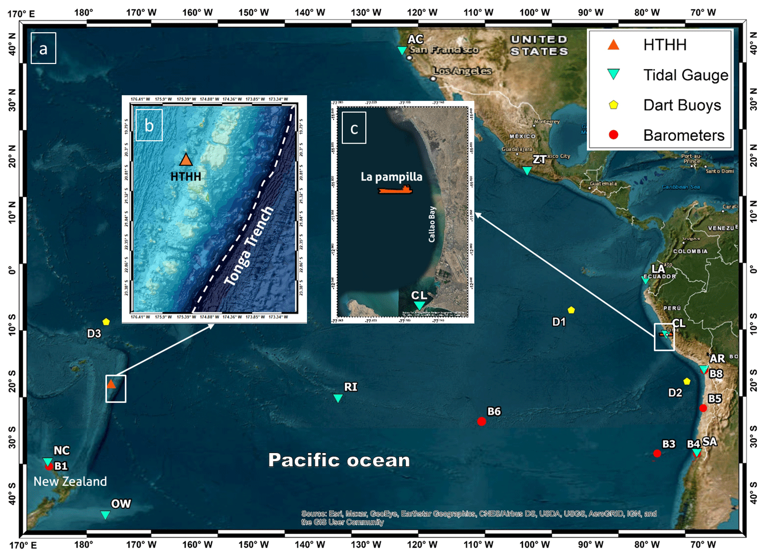
Figure 1(a) Locations of the measuring instruments. Red circles show the atmospheric pressure sensors, the light blue triangles show the tide gauges, and the yellow circles refer to the DART buoys. Panel (b) shows the HTHH volcano (orange triangle) and Tonga Trench location. Panel (c) is the Callao Bay zoom; the orange vessel represents the location of terminal 2 of the port of La Pampilla, Peru.
The deep-water sea-level time series (D1, D2, and D3) were obtained from the DART buoys, which are managed by the Center for Operational Oceanographic Products and Services of the National Oceanic and Atmospheric Administration (NOAA; https://www.ndbc.noaa.gov/, last access: 8 February 2022). Coastal sea-level data used in this study come from tidal stations connected in real time to the Sea Level Station Monitoring Facility of UNESCO's Intergovernmental Oceanographic Commission (IOC; http://www.ioc-sealevelmonitoring.org/, last access: 8 February 2022). The B1 air-pressure data have been obtained from local agents in New Zealand (NIWA; https://niwa.co.nz/, last access: 20 November 2022), and those from stations B3, B4, B5, and B8 came from the Dirección General De Aeronáutica Civil de Chile (DGAC; https://climatologia.meteochile.gob.cl/, last access: 20 March 2023) through the Chilean Meteorological Office.
The sea-level time series were de-tided using bandpass filters of 1.5 min–2.5 h and 2 min–3 h for DART and tide gauge data, respectively, following Lynett et al. (2022). For atmospheric pressure data, a bandpass filter of 1.5 min–2.5 h was used (Table 1). Figure 2 shows the filtered time series. The arrival time was less than 3 h for the B1 sensor in the near field (shape differences are caused by the sample time) and between 8 and 12 h in the far field, about 10 000 km away. The air-pressure time series shows a notable peak of approximately 2 hPa with the “N-wave” pulse shape associated with the leading Lamb wave (Lynett et al., 2022; Omira et al., 2022). The seawater elevation, from deep-water DART sensors, shows tsunami arrival times at two different moments related to the inverse barometer effect due to the leading Lamb wave and the acoustic–gravity waves coupled in ocean (VMT) with values of no more than 10 cm. On the other hand, the tidal gauge shows tsunami wave values higher than 1 m especially in the far-field locations like the Chilean and Peruvian coasts.
Table 1Description of measuring instruments. NDBC signifies the National Data Buoy Center.
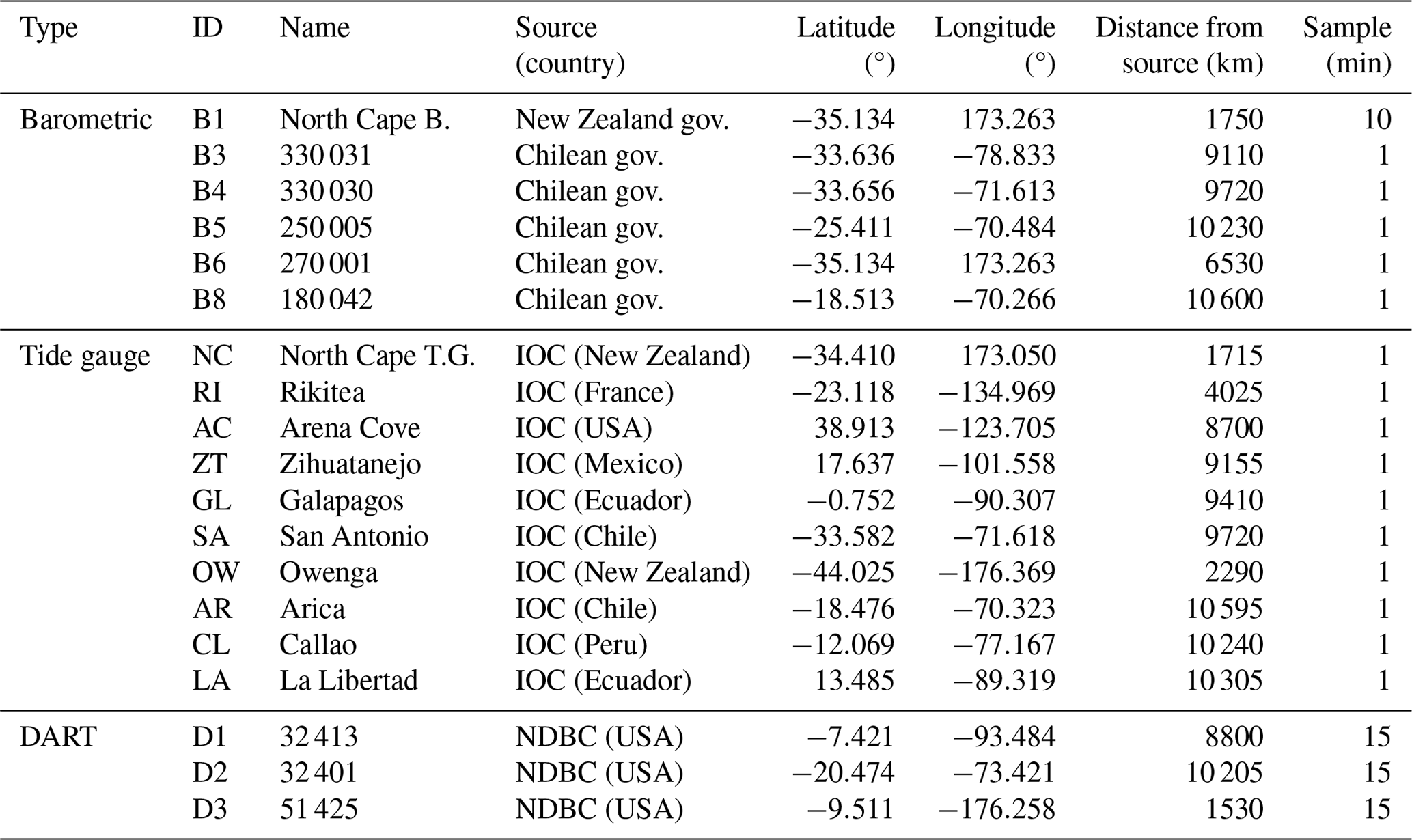
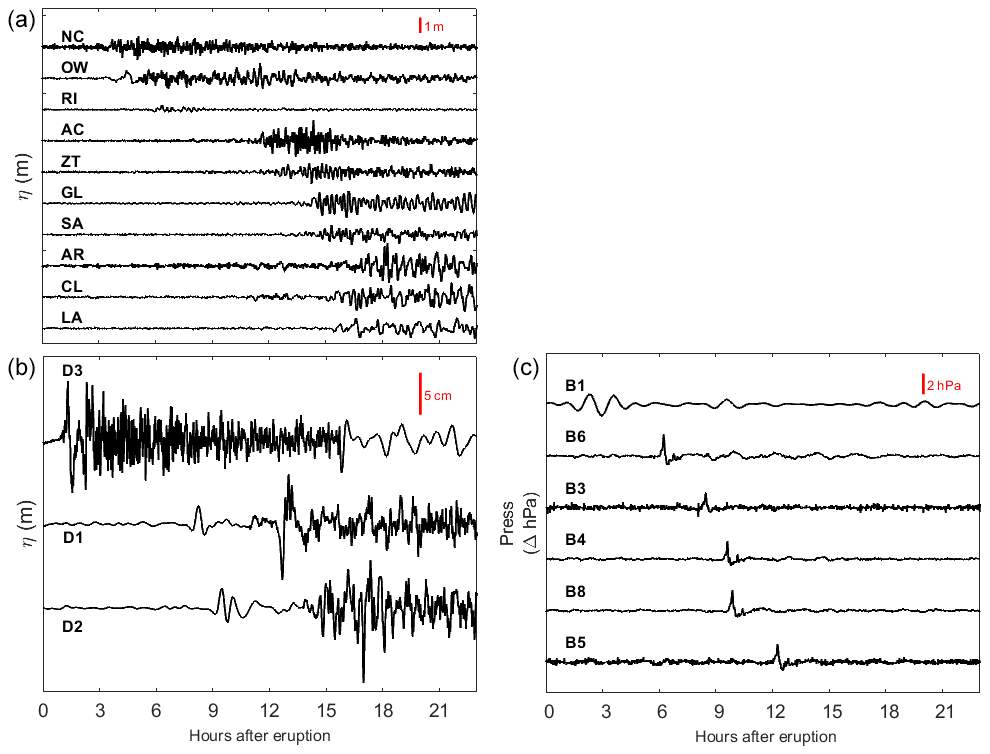
Figure 2De-tided time series. Tide gauge data (a), DART data (b), and air-pressure data (c). Vertical red lines are used to scale the magnitude of the variations in each instrument.
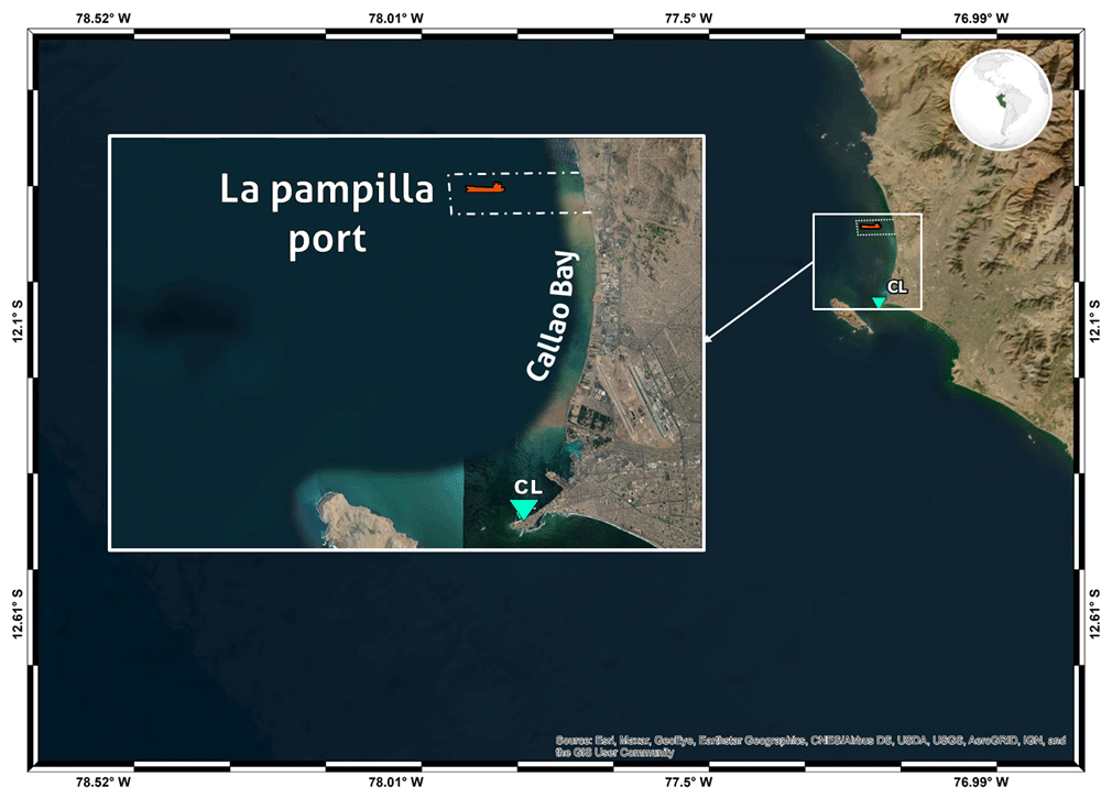
Figure 3Callao Bay and location of the vessel (orange vessel) in the offshore port of La Pampilla, Peru, at coordinates 11°56′ S, 77°11′ W.
2.2 Spectral analysis
Spectral analysis is a practical tool for identifying the characteristic frequencies and energy levels in a time series, particularly when it is composed of the superposition of signals with different frequencies. This method has found extensive application in the study of tsunamis (Abe, 2011; Rabinovich, 1997; Shevchenko et al., 2011; Satake et al., 2013; Baptista et al., 2016; Xu et al., 2022). In the time domain, we use wavelets to perform spectral analysis, allowing the estimation of the evolution of the spectral energy and, consequently, the first instants of energy increase for a given specific period. Wavelet methodology applies a function composed of a complex exponential equation modulated by a Gaussian function for its fitting procedure, which is generally known as a mother function. One of the famous wavelet mother functions is the Morlet function [ψ(t)], which is given by Eq. (1) (Goupillaud et al., 1984):
where f0 is the centre frequency of the wavelet function and t is the time. For the present study, it has been discretized in n sub-octaves per octave with n=50 for better scale resolution and a wavenumber (k0) of 8. Where the spectral energy of the wavelet is defined as . A logarithmic scaling has been performed to obtain an adequate highlighting of spectral energy information as follows:
It means that eps returns the distance from 1.0 to the next largest double-precision number, which is 2−52. In turn, the spectral energy frequency is presented by performing the temporal integration of the wavelet as follows:
2.3 Tsunami propagation model
Although the air–ocean interaction has been recognized as a primary mechanism for the global fast-travelling Tonga 2022 tsunami (Omira et al., 2022), the volcano–ocean interaction provided valid explanations for the near-field observation (Lynett et al., 2022; Pakoksung et al., 2022). As our primary target is Callao Bay, located approximately 10 000 km away from the HTHH volcano (Fig. 3), we only focused on the tsunami induced by the atmospheric disturbances that followed the volcano explosion. The hypothesis of a point-source tsunami reaching the South American coast was ruled out considering the modelling results of a tsunami generated by the underwater explosion of the HTHH volcano (Omira et al., 2022).
To simulate the VMT triggered by the explosion of the HTHH volcano, we used the finite-volume GeoClaw code equipped with atmospheric pressure forcing terms that are handled using the flux-splitting method in momentum balance (Mandli and Dawson, 2014). This numerical code was validated in various meteotsunami studies (Kim and Omira, 2021; Kim et al., 2022; Omira et al., 2022). The determination of atmospheric source terms is based on barometric records from three distinct observations selected from B1, B6, and B8 (see Table 1 for details). To generate the atmospheric input for the tsunami propagation modelling, we adopted an approach where we assumed radial symmetry of atmospheric pressure emanating from HTHH with a constant speed. Specifically, we set the propagation speed at 310 m s−1 and interpolated the atmospheric pressure at each computational grid point using the values from the two closest observed records. The selection of observed records at Kaitaia (New Zealand), 270 001 (Chile), 200 006 (Chile), and Charlotte (US Virgin Islands) was made strategically to capture a diverse range of atmospheric conditions and geographical locations relevant to our study area. These locations were chosen based on their proximity to the region of interest and the availability of reliable barometric records. We acknowledge the importance of validating our atmospheric input against barometric records. We have documented the details of this validation process in our previous work (Omira et al., 2022), where we discuss the consistency between the modelled atmospheric input and observed barometric data.
Our simulations covered an area from 170 to 295° E longitude and from 40° S to 40° N latitude, as obtained from GEBCO (https://www.gebco.net/, last access: 17 November 2022). To effectively simulate sea-level fluctuations induced by atmospheric pressure, we used adaptive mesh refinements (AMRs) based on both atmospheric pressure and sea-level variations. Six levels of AMRs were utilized, beginning with a base resolution of 1° and employing refinement ratios of 5, 6, 4, 4, and 5 at successive levels. We used resolutions as fine as 0.025 arcmin (∼45 m) in areas such as Pampilla, Callao, and La Liberdade while employing a coarser resolution of up to 0.5 arcmin (∼900 m) in other regions to balance computational efficiency with accuracy. To account for the bottom friction, GeoClaw software uses Manning's formulation, and the Manning coefficient of 0.02 was considered in this work. Our simulations were conducted using Madsen's Boussinesq-type equations, with a constant value of (Kim et al., 2017; Madsen and Sørensen, 1992).
The computation was performed on an Intel Core i7-8700 CPU at 3.2 GHz using 10 cores corresponding to 1161 h of propagation time and 119 h of wall time.
2.4 Stresses in moored ship model
Here, we use an analytical model to estimate the loads on a vessel's mooring system under the hydrodynamic effects of a tsunami (Tahar and Kim, 2003; OCIMF, 2010). The vessel is modelled as a rigid body with 6 degrees of freedom (DOFs). The first 3 DOFs are the surge, sway, and heave (x, y and z) of the vessel's centre of gravity (COG), given in the global frame (Fig. 4). The other three are the Euler angles, roll, pitch, and yaw (α, β and γ), which describe the local frame rotation status with respect to the global frame.
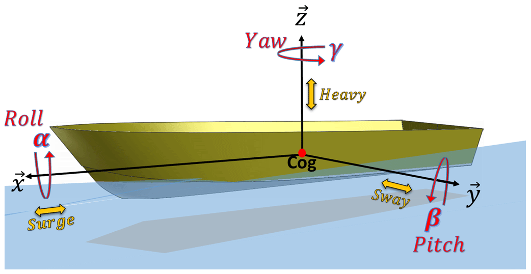
Figure 4Definition of ship motions in 6 degrees of freedom, the yellow ones describing translation and the red ones rotation.
We considered two reference frames, the first of which is a global orthogonal inertial frame (fixed) with its origin located somewhere at the mean water level, where the x axis points eastward and the z axis points upward for the global frame. The second is an orthogonal non-inertial frame, moving with the vessel, with its origin located at the COG. The x axis points toward the bow, while the z axis points upward for the local frame. The roll and pitch initial equilibrium positions are considered to be at 0°.
The model contemplates the vessel's hydromechanics and physics characteristics such as hydrostatic stiffness (which considers both buoyancy and gravity forces), vessel mass (m), metacentric heights (GMt,l), and inertial forces defined by the vessel's moments of inertia around the principal axes (), as well as describing the vessel's stability (Journée and Massie, 2001). The vessel's dynamics are described with the equations of a forced and damped mass–spring system which allows the following initial value problem (Eq. 5):
where Y0 is the initial vessel state vector containing the initial position and the speed of the vessel, B is the damping matrix, G is the stiffness matrix, ξ is defined as the stacking of all the DOFs, ξ0 is the initial equilibrium position, and Fm and Fd are the mooring system forces and the current drag forces (Fig. 5).
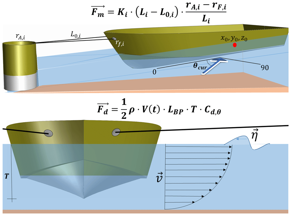
Figure 5Schematic layout of ship mooring system forces Fm and drag forces Fd. The dynamics of the moored vessel are defined with a second-order ordinary differential equation (ODE).
The mooring system Fm is exclusively considered when the movement of the vessel results in a greater increase in the length of the line Li compared to the previous position, as shown in the following Eq. (6):
where Ki includes elastic properties for the ith line, Li is the line length, and rA and rF are the pile and fairlead positions (where the line is tied to the hull). The Morison drag force model (Oh et al., 2020) is utilized to calculate the drag force Fd. The tsunami current at time t is defined by its speed. The current drag force changes depending on the angle of incidence, the , calculated as Eq. (7):
where Cx and Cy are the drag forces on the x and y axes, ρ is the water density, V(t) is the tsunami current velocity, LBP is the length between the perpendicular, T is the vessel's draft, and γ is the yaw DOF. We considers the tsunami current angle θ to be parallel to the vessel's centerline at 0°. Finally, this first-order ODE is integrated with a Runge–Kutta (4, 5) method implemented in the SciPy Python library (Dormand and Prince, 1980; Shampine, 1986).
The model inputs consist of the vessel's dimensions, hydromechanical and mass properties, the ship's berthing scheme (including piles and fairleads coordinates), the line properties (such as young modulus and length), and the temporal tsunami dynamics (including wave and current time series) at the vessel's location. It should be noted that the tsunami dynamics time series were obtained from the dispersive Boussinesq-type numerical model, explained in the previous Sect. 2.3, which solves the equations known as Serre–Green–Naghdi (SGN) instead of the usual shallow seawater elevation (SWE) equations. The SGN equations are still depth-averaged equations, with the same conserved quantities (Berger and LeVeque, 2023). Their numerical results can be used to determine the estimation of current velocities due to tsunamis in harbour environments (Admire et al., 2014; Lynett et al., 2014; Borrero et al., 2015; Ayca et al., 2014). The model outputs the movements in each DOF and the resulting stress, measured in tonnes, for each line throughout the time series.
3.1 Atmospheric and oceanic data analysis
The analysis using wavelets is based on the hypothesis that the atmospheric waves' integral characteristics, such as the periods and propagation velocities, remain reciprocal when resonance is generated between atmospheric and oceanic waves. This allows for the current knowledge extrapolation about atmospheric waves, which have been extensively studied in the literature, and their effect on oceanic tsunami waves.
The results in Figs. 6–8 show the analysis of the recorded atmospheric and sea-level signals, which are composed of three panels for each sensor. The top panel shows the filtered time series of both sea level and atmospheric pressure (blue and orange, respectively). The orange arrow indicates the leading Lamb wave arrival time. The lower panel shows the spectral results (wavelets) of the de-tided series of the ocean surface – the red–blue colour scale marks the highest and lowest energy concentrations, respectively; to the right is the Fourier spectrum obtained from integrating the wavelet over time.
Results in Fig. 6 correspond to the tide gauges NC, OW, and RI; DART buoy D3; and pressure sensor B1 (see Fig. 1 for location). Wavelets consistently show four energy groups for sensor tide gauges NC, OW, and RI and DART buoy D3. These results allows for the identification of the initial characteristics of tsunami waves forced by atmospheric waves, i.e. the arrival times and wave periods.
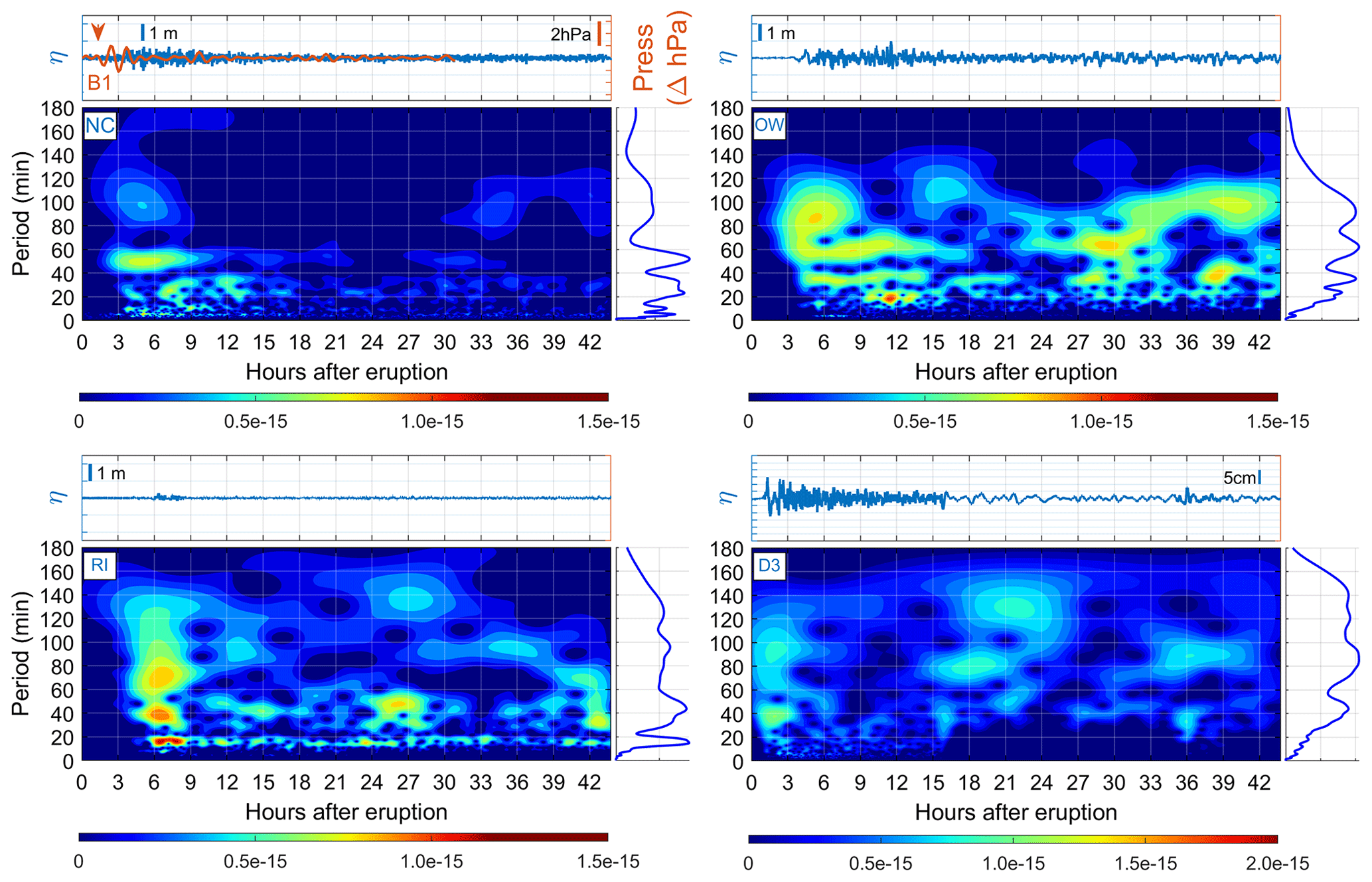
Figure 6Analysis of air-pressure and sea-level records at tide gauges NC (North Cape, New Zealand), OW (Owenga, New Zealand), and RI (Rikitea, France); DART buoy D3 (51 425, NDBC); and air-pressure sensor B1 (North Cape, New Zealand). For each sensor, the time series of the air-pressure sensor (orange line) and tide gauge (blue line) are shown in the upper panel. The orange arrow refers to the arrival time of the leading pressure pulse. The panel to the right of the wavelet is the resulting frequency spectrum (fast Fourier transform – FFT) of the time integration of the wavelet.
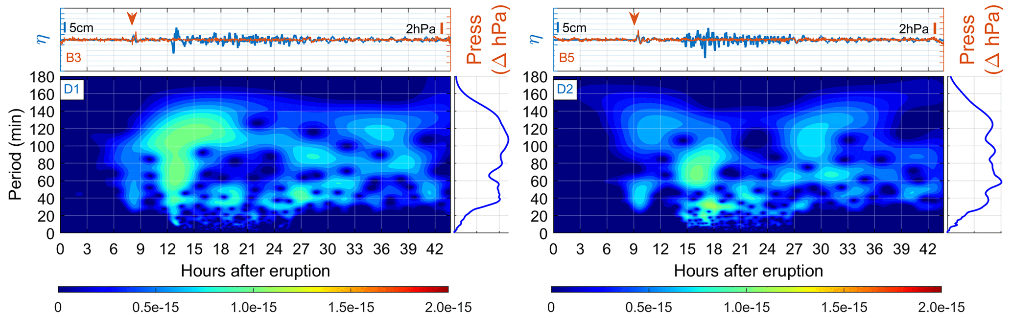
Figure 7Analysis of air-pressure and sea-level records at DART buoys D1 (32 413, NDBC) and D2 (32 401, NDBC) and atmospheric pressure sensors B3 (330 031, Chile) and B5 (250 005, Chile). For each sensor, the filtered time series of the atmospheric pressure sensor (orange line) and tide gauge (blue line) are shown in the upper panel. The orange arrow refers to the arrival of the leading pressure pulse. The right panel of the wavelet is the frequency spectrum resulting from the time integration of the wavelet.
The energy clusters fall within the 5–10, 20–40, 40–60, and 80–120 min periods, so the energy clusters suggest that there were multiple mechanisms that generated the Tonga tsunami waves. These results are consistent with the findings of previous studies (Hu et al., 2023; Kubota et al., 2022; Omira et al., 2022), where tsunami waves with a 1–2 h period were also observed at different tidal gauges when analysing the similar phenomenon that took place in 1883 during the eruption of the Krakatau volcano (Choi et al., 2003; Pelinovsky et al., 2005).
Figure 7 shows far-field results (deep waters near the Peruvian coast) for sensors D1–B3 and D2–B5. Air-pressure time series show the 2 hPa pulse associated with the leading Lamb wave arriving first, followed by second disturbances travelling at more than 200 m s−1 (Hu et al., 2022; Omira et al., 2022). DART buoy wavelets provide more spectral information related to the physical properties of these atmospheric waves coupled in the ocean. For example, DART buoy D2 shows that the first pulse coincides with the leading Lamb wave between 30 and 60 min periods arriving 9 h after the main eruption. Then, there is a group of energy contained in four ranges of periods: (i) about 10 min, (ii) between 20 and 40 min, (iii) between 60 and 90 min, and (iv) between 100 and 140 min. The latter is possibly associated with the air–ocean Proudman resonance that occurred on the Tonga Trench and propagated as common tsunami gravity waves towards the southern American coast (Omira et al., 2022).
Figure 8 shows the spectral results for other locations along the American Pacific coasts. The southern American Pacific instruments are SA–B4 (Chile), AR–B8 (Chile), CL–B5 (Peru), and AL (Ecuador). The sensors in Central and North America are ZT (Mexico) and AC (USA). The wavelets' results in Chile, Mexico, and the USA show several energy groups: one in 40–60 min periods, another group between 20–40 min, and finally energy in periods less than 10 min. Those wavelets exhibit a pattern similar to that observed in deep-water sensors, with a notable difference regarding the absence of periods close to 120 min.
Subsequently, Fig. 8 shows the analysis for sensors LA (Ecuador) and CL–B5 (Peru), 15 km from the vessel accident. The dotted vertical black line on the CL wavelet refers to the moment when the ship's moorings break and the oil spill occurs, according to the captain of the ship Mare Doricum. It can be observed in the CL wavelet that (i) the Lamb wave coupled in the ocean (spectral energy between 30–60 min periods) and (ii) the mooring break moment coincides with the high-period spectral energy (max between 110–130 min period). Additionally, the energy within the 100 to 140 min period is present in deep water (e.g. at DART buoy D1 in Fig. 7) and amplified exclusively in front of the Ecuador and Peru coasts (LA and CL tide gauges).
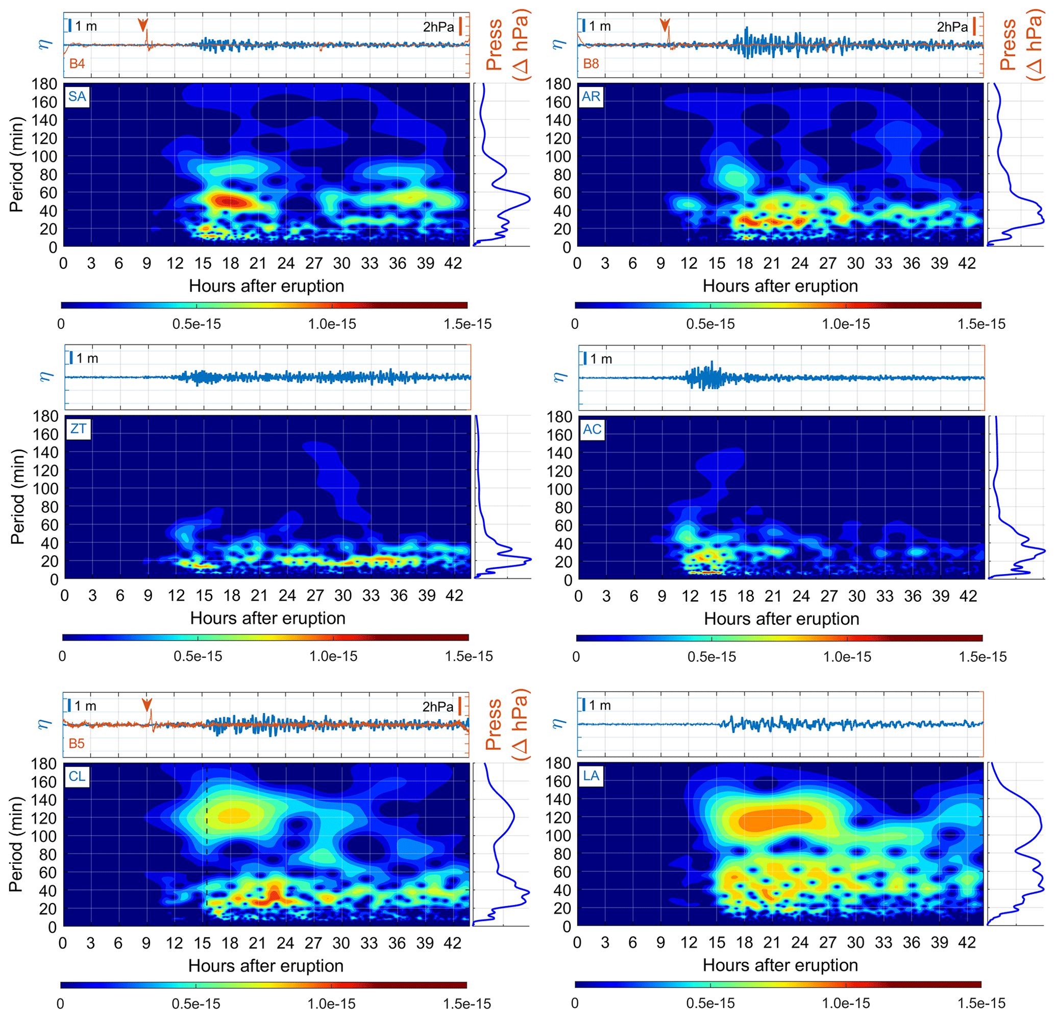
Figure 8Analysis of air-pressure and sea-level records at the tide gauges of SA (San Antonio, Chile), AR (Arica, Chile), ZT (Zihuatanejo, Mexico), AC (California, USA), CL (Callao, Peru), and LA (La Libertad, Ecuador). The upper panel shows the time series of the atmospheric pressure sensor (orange line) and tide gauge (blue line). The orange arrow refers to the arrival of the leading Lamb wave. For the lower panel, we have the wavelet. The dashed vertical black line in the CL wavelet refers to the instant when the vessel's moorings broke at the port of La Pampilla, Peru. The panel to the right of the wavelet is the frequency spectrum.
3.2 Numerical modelling of atmospheric-pressure-induced tsunami waves
The numerical simulations have been calibrated and validated using both far- and near-field instrumental data. After validation, the significance of tsunami-like waves induced by atmospheric acoustic–gravity waves and tsunami-induced waves resulting from the submarine explosion was analysed. We present the results in Fig. 9, which shows the observed and simulated tsunami waveforms near the coast of Peru.
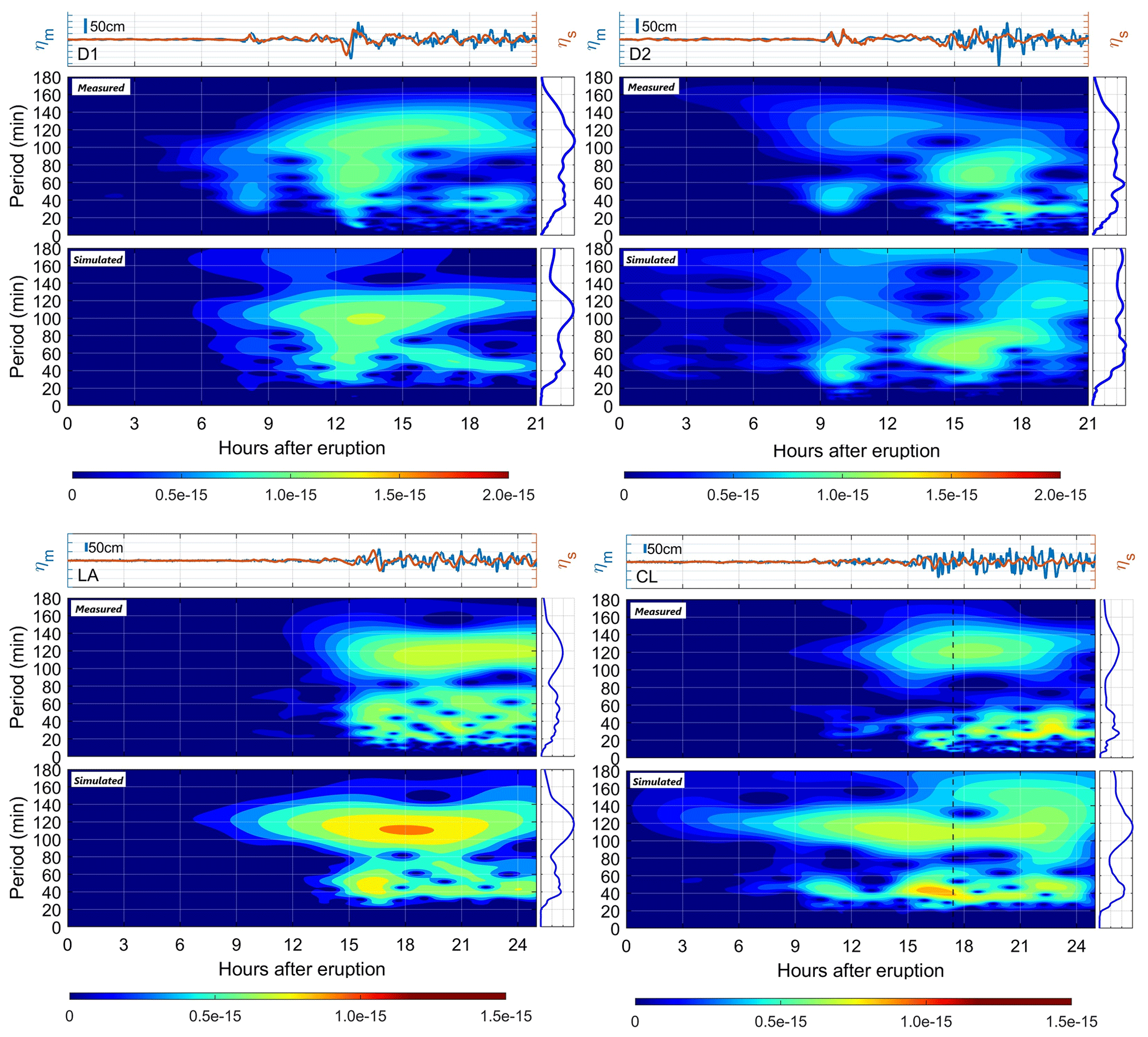
Figure 9Validation of numerical results at DART D1 and D2 buoys and tide gauges CL (Callao, Peru) and LA (La Libertad, Ecuador). For each buoy, the measured (blue line) and simulated (orange line) time series are shown in the upper panel. The lower panel shows the measured free sea surface wavelets (upper wavelet) and numerical simulation (lower wavelet). The dashed vertical black line in CL refers to the instant the vessel mooring breaks in the harbour of La Pampilla, Peru. The panel to the right of each wavelet is the frequency spectrum.
A comparison of observed and simulated tsunami waveforms at DART buoys (D1 and D2) shows that the Boussinesq numerical model correctly reproduces the first tsunami wave. It also fairly reproduces the second train of tsunami waves, likely associated with air–ocean resonance in the deep ocean (near Tonga Trench) and travelling at common tsunami speeds (Omira et al., 2022; Hu et al., 2023; Kubota et al., 2022). In shallow waters, the model correctly reproduces the tide gauges LA and CL (closest to the port of La Pampilla in Peru) like in deep waters.
The correlation results obtained from the numerical validation near the port of La Pampilla are mainly the consequence of detailed information such as bathymetry and atmospheric forcers. The low quantity and quality of the actual measured data near the port lead to the following results:
-
perturbations not accurately captured due to non-linear interactions due to processes such as refraction, diffraction, and reflection;
-
underestimation of the results in the ocean surface wave;
-
underestimation of current velocity.
The wavelets and fast Fourier transform (FFT) show a correct trend of the wave characteristics measured in each sensor, as shown in Fig. 9. Wavelets corresponding to both deep and shallow waters present several groups of waves forced by acoustic waves between 20–40 min periods, 40–60 min periods, and long-period waves of about 120 min (Hu et al., 2023; Kubota et al., 2022; Omira et al., 2022). Likewise, the Fourier spectra also show two distinguished groups of 40–60 and 100–120 min in shallow water.
Compared to the DART buoys, the simulations exhibit similar behaviours because they are located at great depths, where the influence of the bathymetry and the land boundaries is negligible. The simulations demonstrate that tide gauges reveal variations such as earlier arrival times or more energy, possibly associated with local effects and limitations in resolution. Despite these limitations, the model is sufficiently useful for the purpose of the study.
Figure 10 displays simulation results for shallow-water tide gauges GL and SA (located north and south of Peru, respectively), demonstrating that the 120 min period wave is exclusive of the coast of Peru and is likely intensified by local effects. The wavelet analysis indicates that neither the simulated nor the measured waves show a significant amplification of high-period energy, as seen in the sensors situated off the coast of Peru.
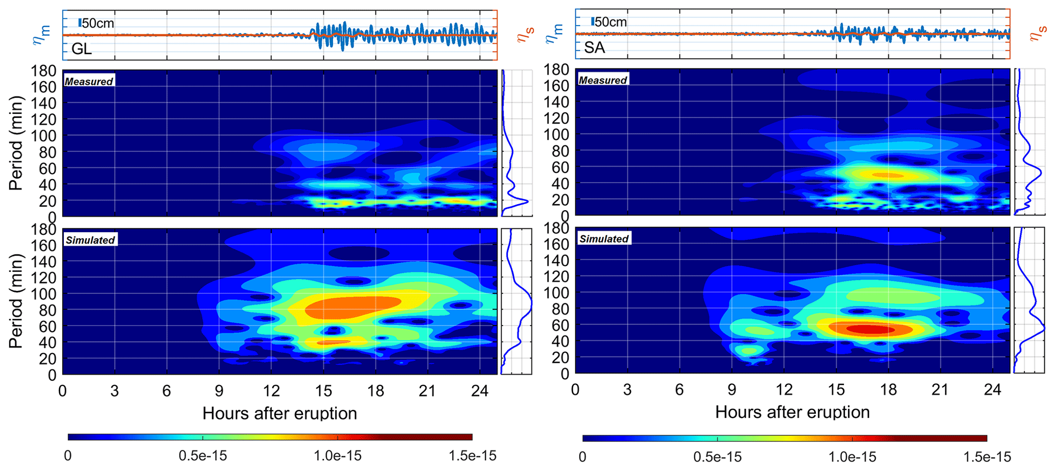
Figure 10Comparisons of the numerical results at the GL (Galapagos, Ecuador) and SA (San Antonio, Chile) tide gauges are shown. For each tide gauge, the measured (blue line) and simulated (orange line) time series are shown in the upper panel. The lower panel has measured (upper wavelet) and simulated (lower wavelet) ocean results. The panel to the right of each wavelet is the frequency spectrum.
3.3 Vessel response due to acoustic and tsunami waves
The model described in Sect. 2.4 was implemented to estimate the mooring stresses due to tsunami hydrodynamic effects produced during the Tonga event. The purpose is to demonstrate the variability in stress levels when exposed to tsunami waves of varying periods and, therefore, different hydrodynamic conditions.
The current velocity and water elevation time series were extracted from the Boussinesq tsunami model, presented in Sect. 2.3 and validated in Sect. 3.2 at coordinates lat −11.932, long −77.181 (Fig. 11a). The velocity of the current and seawater elevation (SWE) input to the mooring line load model are presented in Fig. 11c. The numerical results suggest that the ocean dynamics over time begin to be noticeable 10 h after the eruption, which coincides with the arrival of the leading Lamb wave and with maximums at times close to the time of the rupture accident according to the port authority. The maxima of the current and SWE have values close to 40 cm s−1 and 0.7 m, respectively. On the other hand, the direction of the current suggests a north–south tilting motion, a similar pattern observed during the entire simulation.
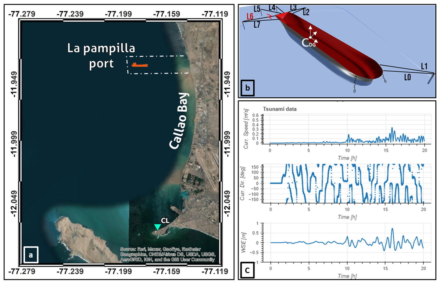
Figure 11Panel (a) shows the location of the tide gauge CL and the port of La Pampilla at Callao Bay, Peru. Panel (b) is the berthing scheme implemented in the mooring line load model, where L6 is the line that broke and caused the instability in the mooring system safety. COG is the centre of gravity of the tanker and origin of the model coordinate system. Panel (c) is the time series extracted from the numerical model at tanker location and inputted in the mooring line load model: upper panel is the current velocity, the middle panel is the current direction, and the lower panel is the variation in the seawater elevation (SWE).
The mooring scheme (Fig. 11b) is similar to the one found in terminal 2 of the port of La Pampilla in Peru during the broken mooring accident. The vessel is moored to five buoys with eight moorings, one forward and four at the stern (in addition to two stern anchors anchored at a depth of 18 m). The line number six (L6 in Fig. 11b) was the one that broke in the actual accident that occurred at the port of La Pampilla 15 h after the eruption of the HTHH volcano.
Tables 2 and 3 present the vessel's description and its hydromechanical characteristics. The entire mooring system schematic and the data used in the model are provided. The vessel used in this study is not the oil tanker Mare Doricum but rather one with comparable physical characteristics. The ship is considered fully loaded throughout the simulation (Fig. 12).
Table 2Description of the vessel used in the mooring stress simulation.
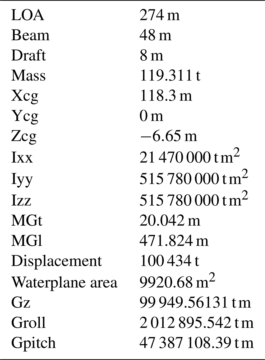
Table 3Description of the mooring system used in the stress simulation.
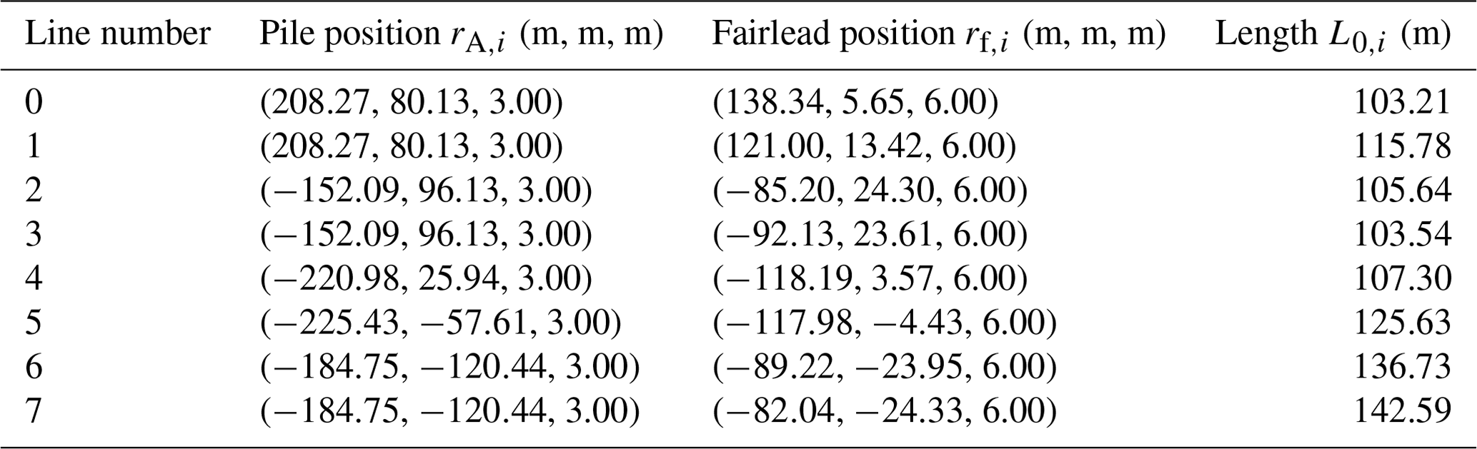
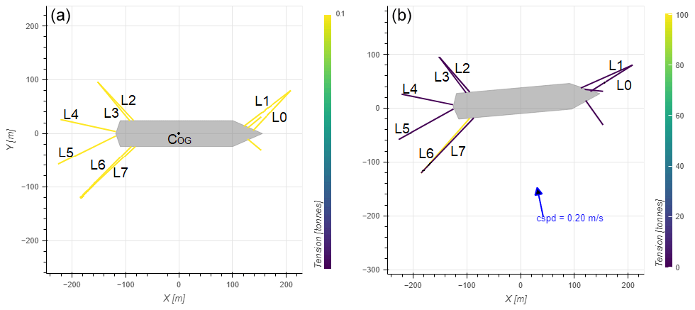
Figure 12On the left (a) is the initial layout with the origin at the ship's COG, and on the right (b) is the layout at the time of mooring breakage, where the yellow and purple colours mark the maximum and minimum stress values, respectively. The cspd (blue arrow) value is the current speed at the time of the breaking of the mooring line.
The results of the DOFs throughout the simulation are presented in Fig. 13. The first instances of ship movement occur about 9 to 10 h after the volcano erupts, coinciding with the arrival of atmospheric waves (VMT), with variations on the order of 2 m, 8 m, and 2° for the surge, sway, and yaw DOFs, respectively, in the movements directly associated with tsunami hydrodynamic loads (López and Iglesias, 2014). Then, 15 h after the eruption, when the 120 min period wave is present and the mooring breaks, further ship motion is generated, drastically increasing the DOF values of the above-mentioned vessel. The model results indicate that the movement was caused by the VMT. The anchored ship aligns with the surge, sway, and yaw, with a maximum deviation of 9 m, 14 m, and 5°, respectively, which is more than enough to produce the breakage of the mooring system according to the port authority of La Pampilla (CPAAAAE, 2023).
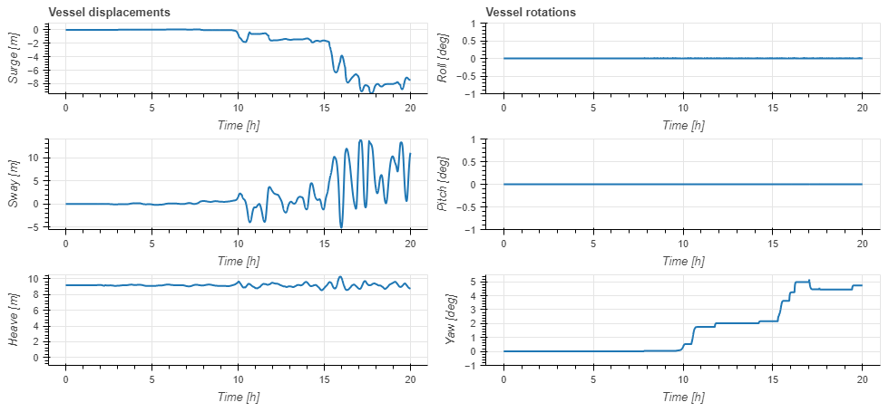
Figure 13Time series of ship 6 degrees of freedom obtained from numerical simulation. Measured in hours after the eruption.
To support the hypothesis that the 120 min long-period wave along the Peruvian coast caused the mooring to break, a comparison was made between the stresses obtained by forcing with the VMT time series and the tsunami caused only by the submarine explosion. The stress results for each line in both cases are shown in Fig. 14. This illustration shows two things. Firstly, with the VMT, the lines that are primarily under stress are the starboard mooring lines number 0, 4, and 6, the latter having the maximum load (96 t), which exceeds the minimum breaking load (MBL) by more than 10 t. The configuration of the mooring layout, tsunami wave direction, and hydrodynamic effects can be potential reasons for the increase in stresses, which could cause the mooring line to break. Secondly, the findings suggest that the VMT results in a significant increase in mooring stresses, exceeding 10 times the levels observed during the tsunami-only event (where the VMT is not included in the simulation). These results suggest that the atmospheric waves generated during the volcanic eruption have triggered a VMT, generating tsunami-like waves that may have affected the mooring safety of vessels berthed in offshore ports in the far field.
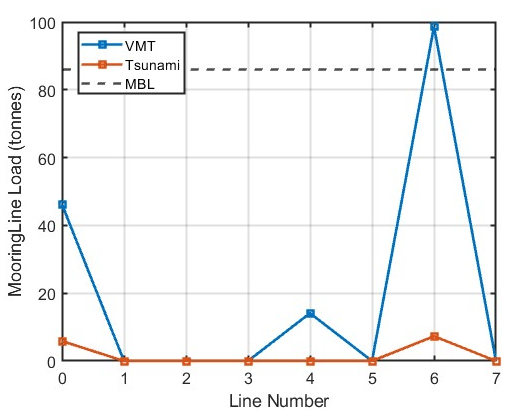
Figure 14Maximum stresses obtained from the simulation at each mooring. Blue and orange lines represent the results of the simulations with and without atmospheric waves, respectively.
The propagation of atmospheric waves and their coupling with the ocean were extensively studied following the Tonga event. Although epistemic uncertainties associated with the event are important, it was possible to understand the main drivers and effects of the volcano-meteorological tsunami (VMT) in the mooring safety of vessels moored in offshore ports in the far field. The air–ocean Proudman resonance in deep water was the driving mechanism that caused long-period gravitational waves (which had very similar characteristics to those of a tectonic-source tsunami) to travel along the Pacific Ocean and affect the offshore port La Pampilla in the far field.
There is evidence that the potential of the explosion-induced atmospheric waves magnify tsunamis once they pass over deep-ocean regions. The second train of tsunami-like waves that arrived at the Peruvian coast and affected the mooring safety was generated due to Proudman resonance between acoustic–gravity waves with ocean–gravity waves, which produced an air–ocean energy transfer that led to an increase in tsunami energy in the far field instead of losing it. This happened near the Tonga Trench in the propagation direction of South America (Fig. 3c in Omira et al., 2022).
The presence of the high-period waves exclusively at the tide gauges of Peru and Ecuador (CL and LA, respectively) could be explained by several processes associated with shoaling. These processes could include the width and slope of the continental shelf (which is wider on the Peruvian coast than on the Chilean coast, for example) and the effects associated with topographic boundaries and their geometry, such as the natural bay oscillation modes.
The spectral analysis results establish the influence of the atmospheric waves generated by the HTHH volcano. Considering that the 120 min long-period waves were associated with the air–ocean resonance of the Tonga event and that numerical simulations additionally show the mooring line stress using the VMT time series, it is possible to conclude that the Tonga tsunami caused the overstressing and subsequent accident in the port of La Pampilla, Peru.
Hydrodynamic loads on the vessel's hull due to tsunamigenic phenomena can threaten the stability of moored vessels. These loads are mainly due to drag forces (driven by the tsunami kinetic energy) that affect ship stability. Based on the ship DOFs, the results suggest that VMTs affect mainly the horizontal plane motions: two associated with displacements (sway and surge) and the other with the angle of rotation around its vertical axis (yaw). This is likely explained by the large amount of kinetic energy that tsunamis have in their propagation, which travel at high speed but with little wave elevation. The VMT produced during the Tonga 2022 event was accompanied by long-period waves and currents, which could affect the stability of the mooring system in the port of La Pampilla, Peru.
The hydrodynamic effects of very long-period tsunami waves can generate damage similar to that of tsunamis of tectonic origin, affecting elements such as infrastructure, vessels, merchandise, and people in port environments.
Final considerations
Coastal and port infrastructure is not prepared to respond preventively to these Tonga-type tsunamis, leaving them “unprotected”, as tsunami warnings are not issued once a volcano eruption is known. Furthermore, in the analysed event, the initial ocean disturbance arrived earlier than anticipated because the atmospheric waves produced a VMT that travelled at sonic velocity. This statement holds relevance as state and international authorities are responsible for maritime safety and the creation of cautions, warnings, and suggestions to aid distinct users in coastal and offshore locations.
This event showed the need for tsunami early warning systems (TWSs) to be prepared to include atmospheric waves and detect them from existing monitoring sensors. In addition, standard operational procedures need to include protocols for these events to avoid damage to port facilities and ships, such as the breaking of moorings and ship collisions. These events can also generate local flooding increasingly far away from the origin and affect the population and coastal infrastructure (cities, nuclear reactors, petrochemical industry, etc.). Therefore, efforts towards the incorporation of tsunamis caused by volcanic acoustic waves in tsunami warning systems are needed.
The coupled GeoClaw–atmospheric air–pressure code is available on request from the corresponding co-author, Rachid Omira (Omira et al., 2022). The tsunami numerical code GeoClaw is available on the Clawpack website (https://www.clawpack.org/geoclaw.html, Clawpack, 2023). The mooring stress calculation code can be obtained from the corresponding main author (the mooring effort model is not completely open access because it has been created under the authorship of the company IHCantabria).
Tidal gauge sea-level datasets are available from the UNESCO Intergovernmental Oceanographic Commission (IOC) Sea Level Station Monitoring Facility (http://www.ioc-sealevelmonitoring.org, IOC, 2022). DART buoys are available from the Center for Operational Oceanographic Products and Services of the National Oceanic and Atmospheric Administration (NOAA) (https://www.ncei.noaa.gov/maps/hazards/, NOAA, 2022). The New Zealand air-pressure data are available from NIWA (https://niwa.co.nz/climate-and-weather/obtaining-climate-data-niwa, NIWA, 2023). All other atmospheric data were obtained by the Dirección Meteorológica de Chile (DGAC) (https://climatologia.meteochile.gob.cl/application/informacion/buscadorEstaciones, DGAC, 2023). The Pacific bathymetric data are available from the General Bathymetric Chart of the Oceans (GEBCO) (https://download.gebco.net/, GEBCO, 2022).
MG and IAQ: supervision and methodology; JK and RO: wave simulations; MAB and RO: revision. All authors have read and agreed to the published version of the manuscript.
At least one of the (co-)authors is a member of the editorial board of Natural Hazards and Earth System Sciences. The peer-review process was guided by an independent editor, and the authors also have no other competing interests to declare.
Publisher's note: Copernicus Publications remains neutral with regard to jurisdictional claims made in the text, published maps, institutional affiliations, or any other geographical representation in this paper. While Copernicus Publications makes every effort to include appropriate place names, the final responsibility lies with the authors.
This research was supported by an FPU (Formación de Profesorado Universitario) grant from the Spanish Ministry of Science and Innovation (MCINN) to the first author. We are grateful to the Ocean Energy and Offshore Engineering Group of IHCantabria for the model of mooring stresses. In addition, the authors of this work would like to thank the various state institutions that have provided measured atmospheric data mentioned in Sect. 2: IDEAM (Colombia), SENAMHI (Peru), DGAC (Chile), NIWA (New Zealand), NOAA (USA), and IOC.
This research has been supported by the Spanish Ministry of Science and Innovation (MCINN) (grant no. FPU2021-05272).
This paper was edited by Ira Didenkulova and reviewed by Efim Pelinovsky and one anonymous referee.
Abe, K.: Synthesis of a Tsunami Spectrum in a Semi-Enclosed Basin Using Its Background Spectrum, Pure Appl. Geophys., 168, 1101–1112, https://doi.org/10.1007/s00024-010-0222-x, 2011.
Admire, A. R., Dengler, L. A., Crawford, G. B., Uslu, B. U., Borrero, J. C., Greer, S. D., and Wilson, R. I.: Observed and Modeled Currents from the Tohoku-oki, Japan and other Recent Tsunamis in Northern California, Pure Appl. Geophys., 171, 3385–3403, https://doi.org/10.1007/s00024-014-0797-8, 2014.
Antonopoulos, J.: The great Minoan eruption of Thera volcano and the ensuing tsunami in the Greek Archipelago, Nat. Hazards, 5, 153–168, https://doi.org/10.1007/BF00127003, 1992.
Ayca, A. and Lynett, P. J.: Effect of tides and source location on nearshore tsunami-induced currents, J. Geophys. Res.-Oceans, 121, 8807–8820, https://doi.org/10.1002/2016JC012435, 2016.
Ayca, A. and Lynett, P. J.: Debris and Vessel Transport due to Tsunami Currents in Ports and Harbors, Coast. Eng. Proc., 68, 68–68, https://doi.org/10.9753/icce.v36.currents.68, 2018.
Ayca, A. and Lynett, P. J.: Modeling the motion of large vessels due to tsunami-induced currents, Ocean Eng., 236, 109487, https://doi.org/10.1016/j.oceaneng.2021.109487, 2021.
Ayca, A., Lynett, P., Borrero, J., Miller, K., and Wilson, R.: Numerical and Physical Modeling of Localized Tsunami-Induced Currents in Harbors, Coast. Eng. Proc., 1, 6, https://doi.org/10.9753/icce.v34.currents.6, 2014.
Baptista, M. A., Miranda, J. M., Batlló, J., Lisboa, F., Luis, J., and Maciá, R.: New study on the 1941 Gloria Fault earthquake and tsunami, Nat. Hazards Earth Syst. Sci., 16, 1967–1977, https://doi.org/10.5194/nhess-16-1967-2016, 2016.
Belousov, A., Voight, B., Belousova, M., and Muravyev, Y.: Tsunamis generated by subaquatic volcanic explosions: Unique data from 1996 Eruption in Karymskoye Lake, Kamchatka, Russia, Pure Appl. Geophys., 157, 1135–1143, https://doi.org/10.1007/s000240050021, 2000.
Berger, M. J. and LeVeque, R. J.: Implicit Adaptive Mesh Refinement for Dispersive Tsunami Propagation, SIAM J. Sci. Comput., 46, B554–B578, https://doi.org/10.1137/23M1585210, 2023.
Borrero, J. C., Lynett, P. J., and Kalligeris, N.: Tsunami currents in ports, Philos. T. R. Soc. A, 373, 20140372, https://doi.org/10.1098/rsta.2014.0372, 2015.
Center for Operational Oceanographic Products and Services by the National Oceanic and Atmospheric Administration (NOAA): Deep-ocean Assessment and Reporting of Tsunamis (DART), https://www.ncei.noaa.gov/maps/hazards/, 8 February 2022.
Choi, B. H., Pelinovsky, E., Kim, K. O., and Lee, J. S.: Simulation of the trans-oceanic tsunami propagation due to the 1883 Krakatau volcanic eruption, Nat. Hazards Earth Syst. Sci., 3, 321–332, https://doi.org/10.5194/nhess-3-321-2003, 2003.
Clawpack: GeoClaw tsunami numerical code, http://www.clawpack.org, last access: 24 December 2023.
CNAT: https://www.tvperu.gob.pe/noticias/nacionales/cnat-no-existe-alerta-de-tsunami-en-el-litoral-peruano, last access: 6 February 2022.
CPAAAAE: Informe Final sobre las acciones de los funcionarios públicos y privados que ocasionaron el derrame de petróleo de la Empresa Multinacional REPSOL YPF S. A., Lima, 421 pp., 2023.
Dirección General De Aeronáutica Civil/Dirección Meteorológica de Chile (DGAC): Catastro de Estaciones del Sistema SACLIM, https://climatologia.meteochile.gob.cl/application/informacion/buscadorEstaciones, last access: 20 March 2023.
Dogan, G. G., Yalciner, A. C., Annunziato, A., Yalciner, B., and Necmioglu, O.: Global propagation of air pressure waves and consequent ocean waves due to the January 2022 Hunga Tonga-Hunga Ha'apai eruption, Ocean Eng., 267, 113174, https://doi.org/10.1016/j.oceaneng.2022.113174, 2023.
Dormand, J. R. and Prince, P. J.: A family of embedded Runge-Kutta formulae, J. Comput. Appl. Math., 6, 19–26, https://doi.org/10.1016/0771-050X(80)90013-3, 1980.
Falvard, S., Paris, R., Belousova, M., Belousov, A., Giachetti, T., and Cuven, S.: Scenario of the 1996 volcanic tsunamis in Karymskoye Lake, Kamchatka, inferred from X-ray tomography of heavy minerals in tsunami deposits, Mar. Geol., 396, 160–170, https://doi.org/10.1016/j.margeo.2017.04.011, 2018.
General Bathymetric Chart of the Oceans (GEBCO): Global Bathymetric Data, https://download.gebco.net/, last access: 17 November 2022.
Goupillaud, P., Grossmann, A., and Morlet, J.: Cycle-octave and related transforms in seismic signal analysis, Geoexploration, 23, 85–102, https://doi.org/10.1016/0016-7142(84)90025-5, 1984.
Hayward, M. W., Whittaker, C. N., Lane, E. M., Power, W. L., Popinet, S., and White, J. D. L.: Multilayer modelling of waves generated by explosive subaqueous volcanism, Nat. Hazards Earth Syst. Sci., 22, 617–637, https://doi.org/10.5194/nhess-22-617-2022, 2022.
Hu, G., Li, L., Ren, Z., and Zhang, K.: The characteristics of the 2022 Tonga volcanic tsunami in the Pacific Ocean, Nat. Hazards Earth Syst. Sci., 23, 675–691, https://doi.org/10.5194/nhess-23-675-2023, 2023.
Hu, Y., Li, Z., Wang, L., Chen, B., Zhu, W., Zhang, S., Du, J., Zhang, X., Yang, J., Zhou, M., Liu, Z., Wang, S., Miao, C., Zhang, L., and Peng, J.: Rapid Interpretation and Analysis of the 2022 Eruption of Hunga Tonga-Hunga Ha'apai Volcano with Integrated Remote Sensing Techniques, Wuhan Daxue Xuebao (Xinxi Kexue Ban)/Geomatics Inf. Sci. Wuhan Univ. [J], 47, 242–251, https://doi.org/10.13203/J.WHUGIS20220050, 2022.
Imamura, F., Suppasri, A., Arikawa, T., Koshimura, S., Satake, K., and Tanioka, Y.: Preliminary Observations and Impact in Japan of the Tsunami Caused by the Tonga Volcanic Eruption on January 15, 2022, Pure Appl. Geophys., 179, 1549–1560, https://doi.org/10.1007/s00024-022-03058-0, 2022.
INDECI: https://www.gob.pe/institucion/indeci/noticias/576687- inician-acciones-de-respuesta-luego-de-oleajes-en-el-litoral, last access: 22 April 2024.
Inoue, Y., Rafiqul Islam, M., and Murai, M.: Effect of wind, current and non-linear second order drift forces on a moored multi-body system in an irregular sea, in: Oceans Conference Record (IEEE), Honolulu, HI, USA, 5–8 November 2001, 1915–1922, https://doi.org/10.1109/oceans.2001.968139, 2001.
Journée, J. M. J. and Massie, W. W.: Offshore Hydromechanics, 1st edn., https://ocw.tudelft.nl/courses/offshore-hydromechanics/ (last access: 28 November 2023), 2001.
Kienle, J., Kowalik, Z., and Murty, T. S.: Tsunamis generated by eruptions from Mount St. Augustine Volcano, Alaska, Science , 236, 1442–1447, https://doi.org/10.1126/science.236.4807.1442, 1987.
Kim, J. and Omira, R.: The 6–7 July 2010 meteotsunami along the coast of Portugal: insights from data analysis and numerical modelling, Nat. Hazards, 106, 1397–1419, https://doi.org/10.1007/s11069-020-04335-8, 2021.
Kim, J., Pedersen, G. K., Løvholt, F., and LeVeque, R. J.: A Boussinesq type extension of the GeoClaw model – a study of wave breaking phenomena applying dispersive long wave models, Coast. Eng., 122, 75–86, https://doi.org/10.1016/j.coastaleng.2017.01.005, 2017.
Kim, J., Choi, B. J., and Omira, R.: On the Greenspan resurgence of meteotsunamis in the Yellow Sea—insights from the newly discovered 11–12 June 2009 event, Nat. Hazards, 114, 1323–1340, https://doi.org/10.1007/s11069-022-05427-3, 2022.
Kirby, J. T., Grilli, S. T., Horrillo, J., Liu, P. L.-F., Nicolsky, D., Abadie, S., Ataie-Ashtiani, B., Castro, M. J., Clous, L., Escalante, C., Fine, I., González-Vida, J. M., Løvholt, F., Lynett, P., Ma, G., Macías, J., Ortega, S., Shi, F., Yavari-Ramshe, S., and Zhang, C.: Validation and inter-comparison of models for landslide tsunami generation, Ocean Model., 170, 101943, https://doi.org/10.1016/j.ocemod.2021.101943, 2022.
Kubota, T., Saito, T., and Nishida, K.: Global fast-traveling tsunamis driven by atmospheric Lamb waves on the 2022 Tonga eruption, Science, 377, 91–94, https://doi.org/10.1126/science.abo4364, 2022.
López, M. and Iglesias, G.: Long wave effects on a vessel at berth, Appl. Ocean Res., 47, 63–72, https://doi.org/10.1016/j.apor.2014.03.008, 2014.
Lynett, P., McCann, M., Zhou, Z., Renteria, W., Borrero, J., Greer, D., Fa'anunu, O., Bosserelle, C., Jaffe, B., La Selle, S., Ritchie, A., Snyder, A., Nasr, B., Bott, J., Graehl, N., Synolakis, C., Ebrahimi, B., and Cinar, G. E.: Diverse tsunamigenesis triggered by the Hunga Tonga-Hunga Ha'apai eruption, Nature, 609, 728–733, https://doi.org/10.1038/s41586-022-05170-6, 2022.
Lynett, P. J., Borrero, J. C., Weiss, R., Son, S., Greer, D., and Renteria, W.: Observations and modeling of tsunami-induced currents in ports and harbors, Earth Planet. Sc. Lett., 327–328, 68–74, https://doi.org/10.1016/j.epsl.2012.02.002, 2012.
Lynett, P. J., Borrero, J., Son, S., Wilson, R., and Miller, K.: Assessment of the tsunami-induced current hazard, Geophys. Res. Lett., 41, 2048–2055, https://doi.org/10.1002/2013GL058680, 2014.
Madsen, P. A. and Sørensen, O. R.: A new form of the Boussinesq equations with improved linear dispersion characteristics. Part 2. A slowly-varying bathymetry, Coast. Eng., 18, 183–204, https://doi.org/10.1016/0378-3839(92)90019-Q, 1992.
Mandli, K. T. and Dawson, C. N.: Adaptive Mesh Refinement for Storm Surge, Ocean Model., 75, 36–50, https://doi.org/10.1016/j.ocemod.2014.01.002, 2014.
Matoza, R. S., Fee, D., Assink, J. D., Iezzi, A. M., Green, D. N., Kim, K., Toney, L., Lecocq, T., Krishnamoorthy, S., Lalande, J. M., Nishida, K., Gee, K. L., Haney, M. M., Ortiz, H. D., Brissaud, Q., Martire, L., Rolland, L., Vergados, P., Nippress, A., Park, J., Shani-Kadmiel, S., Witsil, A., Arrowsmith, S., Caudron, C., Watada, S., Perttu, A. B., Taisne, B., Mialle, P., Le Pichon, A., Vergoz, J., Hupe, P., Blom, P. S., Waxler, R., De Angelis, S., Snively, J. B., Ringler, A. T., Anthony, R. E., Jolly, A. D., Kilgour, G., Averbuch, G., Ripepe, M., Ichihara, M., Arciniega-Ceballos, A., Astafyeva, E., Ceranna, L., Cevuard, S., Che, I. Y., De Negri, R., Ebeling, C. W., Evers, L. G., Franco-Marin, L. E., Gabrielson, T. B., Hafner, K., Harrison, R. G., Komjathy, A., Lacanna, G., Lyons, J., Macpherson, K. A., Marchetti, E., McKee, K. F., Mellors, R. J., Mendo-Pérez, G., Mikesell, T. D., Munaibari, E., Oyola-Merced, M., Park, I., Pilger, C., Ramos, C., Ruiz, M. C., Sabatini, R., Schwaiger, H. F., Tailpied, D., Talmadge, C., Vidot, J., Webster, J., and Wilson, D. C.: Atmospheric waves and global seismoacoustic observations of the January 2022 Hunga eruption, Tonga, Science, 377, 95–100, https://doi.org/10.1126/science.abo7063, 2022.
NIWA: NIWA's climate, freshwater and marine science/ The National Climate Database (New Zealand), https://niwa.co.nz/climate-and-weather/obtaining-climate-data-niwa, last access: 20 March 2023.
OCIMF: Estimating The Environmental Loads On Anchoring Systems, Oil Companies International Marine Forum, London, 33 pp., ISBN 978-1856094047, 2010.
Oh, M. J., Ham, S. H., and Ku, N.: The coefficients of equipment number formula of ships, J. Mar. Sci. Eng., 8, 1–11, https://doi.org/10.3390/jmse8110898, 2020.
Ohgaki, K., Yoneyama, H., and Suzuki, T.: Evaluation on Safety of Moored Ships and Mooring Systems for a Tsunami Attack, Oceans 2008 – MTS/IEEE Kobe Techno-Ocean, Kobe, Japan, 8–11 April 2008, 1–6, https://doi.org/10.1109/OCEANSKOBE.2008.4530986, 2008.
Omira, R., Ramalho, R. S., Kim, J., González, P. J., Kadri, U., Miranda, J. M., Carrilho, F., and Baptista, M. A.: Global Tonga tsunami explained by a fast-moving atmospheric source, Nature, 609, 734–740, https://doi.org/10.1038/s41586-022-04926-4, 2022.
Pakoksung, K., Suppasri, A., and Imamura, F.: The near-field tsunami generated by the 15 January 2022 eruption of the Hunga Tonga-Hunga Ha'apai volcano and its impact on Tongatapu, Tonga, Sci. Rep.-UK, 12, 15187, https://doi.org/10.1038/s41598-022-19486-w, 2022.
Pararas-Carayannis, G.: The tsunami generated from the eruption of the volcano of Santorin in the Bronze Age, Nat. Hazards, 5, 115–123, https://doi.org/10.1007/BF00127000, 1992.
Pararas-Carayannis, G.: Volcanic tsunami generating source mechanisms in the eastern Caribbean region, Sci. Tsunami Hazards, 22, 74–114, 2004.
Paris, R.: Source mechanisms of volcanic tsunamis, Philos. T. Roy. Soc. A, 373, 20140380, https://doi.org/10.1098/rsta.2014.0380, 2015.
Paris, R., Switzer, A. D., Belousova, M., Belousov, A., Ontowirjo, B., Whelley, P. L., and Ulvrova, M.: Volcanic tsunami: A review of source mechanisms, past events and hazards in Southeast Asia (Indonesia, Philippines, Papua New Guinea), Nat. Hazards, 70, 447–470, https://doi.org/10.1007/s11069-013-0822-8, 2014.
Pelinovsky, E., Choi, B. H., Stromkov, A., Didenkulova, I., and Kim, H. S.: Analysis of Tide-Gauge Records of the 1883 Krakatau Tsunami, Adv. Nat. Technol. Haz., 23, 57–77, https://doi.org/10.1007/1-4020-3331-1_4, 2005.
Proudman, J.: The Effects on the Sea of Changes in Atmospheric Pressure, Geophys. J. Int., 2, 197–209, https://doi.org/10.1111/J.1365-246X.1929.TB05408.X, 1929.
Rabinovich, A. B.: Spectral analysis of tsunami waves: Separation of source and topography effects, J. Geophys. Res.-Oceans, 102, 12663–12676, https://doi.org/10.1029/97JC00479, 1997.
Ramírez-Herrera, M. T., Coca, O., and Vargas-Espinosa, V.: Tsunami Effects on the Coast of Mexico by the Hunga Tonga-Hunga Ha'apai Volcano Eruption, Tonga, Pure Appl. Geophys., 179, 1117–1137, https://doi.org/10.1007/S00024-022-03017-9, 2022.
Sakakibara, S., Takeda, S., Iwamoto, Y., and Kubo, M.: A hybrid potential theory for predicting the motions of a moored ship induced by large-scaled tsunami, Ocean Eng., 37, 1564–1575, https://doi.org/10.1016/J.OCEANENG.2010.09.005, 2010.
Satake, K., Rabinovich, A. B., Dominey-Howes, D., and Borrero, J. C.: Introduction to “Historical and Recent Catastrophic Tsunamis in the World: Volume I. The 2011 Tohoku Tsunami”, Pure Appl. Geophys., 170, 955–961, https://doi.org/10.1007/s00024-012-0615-0, 2013.
Shampine, L. F.: Some Practical Runge-Kutta Formulas, Math. Comput., 46, 135, https://doi.org/10.2307/2008219, 1986.
Shevchenko, G., Shishkin, A., Bogdanov, G., and Loskutov, A.: Tsunami Measurements in Bays of Shikotan Island, Pure Appl. Geophys., 168, 2011–2021, https://doi.org/10.1007/s00024-011-0284-4, 2011.
Shigeki, S. and Masayoshi, K.: Initial attack of large-scaled tsunami on ship motions and mooring loads, Ocean Eng., 36, 145–157, https://doi.org/10.1016/j.oceaneng.2008.09.010, 2009.
SPDA Actualidad Ambiental: https://www.actualidadambiental.pe/ derrame-petroleo-cronologia-de-lo-sucedido-segun-el-capitan- del-buque-mare-doricum-video/, last access: 1 March 2024.
Tahar, A. and Kim, M. H.: Hull/mooring/riser coupled dynamic analysis and sensitivity study of a tanker-based FPSO, Appl. Ocean Res., 25, 367–382, https://doi.org/10.1016/j.apor.2003.02.001, 2003.
Terry, J. P., Goff, J., Winspear, N., Bongolan, V. P., and Fisher, S.: Tonga volcanic eruption and tsunami, January 2022: globally the most significant opportunity to observe an explosive and tsunamigenic submarine eruption since AD 1883 Krakatau, Geosci. Lett., 9, 24, https://doi.org/10.1186/s40562-022-00232-z, 2022.
The UNESCO Intergovernmental Oceanographic Commission (IOC): Sea level station monitoring facility, https://www.ioc-sealevelmonitoring.org/map.php, 8 February 2022.
Thomson, R. E., Rabinovich, A. B., Fine, I. V., Sinnott, D. C., McCarthy, A., Sutherland, N. A. S., and Neil, L. K.: Meteorological tsunamis on the coasts of British Columbia and Washington, Phys. Chem. Earth, 34, 971–988, https://doi.org/10.1016/j.pce.2009.10.003, 2009.
Tonga Volcanic Eruption and Tsunami: https://appliedsciences.nasa.gov/what-we-do/disasters/disasters-activations/tonga-volcanic-eruption-tsunami-2022, last access: 15 December 2022.
UNESCO/IOC: Sea level station monitoring facility, Flanders Marine Institute (VLIZ), Intergovernmental Oceanographic Commission (IOC), Sea level station monitoring facility, https://doi.org/10.14284/482, 2021.
Vergoz, J., Hupe, P., Listowski, C., Le Pichon, A., Garcés, M. A., Marchetti, E., Labazuy, P., Ceranna, L., Pilger, C., Gaebler, P., Näsholm, S. P., Brissaud, Q., Poli, P., Shapiro, N., De Negri, R., and Mialle, P.: IMS observations of infrasound and acoustic-gravity waves produced by the January 2022 volcanic eruption of Hunga, Tonga: A global analysis, Earth Planet. Sc. Lett., 591, 117639, https://doi.org/10.1016/J.EPSL.2022.117639, 2022.
Wilson, R., Lynett, P., Eskijian, M., Miller, K., LaDuke, Y., Curtis, E., Hornick, M., Keen, A., and Ayca, A.: Tsunami Hazard Analysis and Products for Harbors in California, in: Tsunami Hazards: Innovations in Mapping, Modeling, and Outreach, in: Geological Society of America Annual Meeting in Seattle, Washington, 23 October 2017, 49-6, https://doi.org/10.1130/abs/2017am-306344, 2017.
World Bank: Report Estimates Damages at US90M, https://www.worldbank.org/en/news/press-release/ 2022/02/14/tonga-volcanic-eruption-and-tsunami-world-bank- disaster-assessment-report-estimates-damages-at-us-90m, last access: 28 February 2024.
Wright, C. J., Hindley, N. P., Alexander, M. J., Barlow, M., Hoffmann, L., Mitchell, C. N., Prata, F., Bouillon, M., Carstens, J., Clerbaux, C., Osprey, S. M., Powell, N., Randall, C. E., and Yue, J.: Surface-to-space atmospheric waves from Hunga Tonga–Hunga Ha'apai eruption, Nature, 609, 741–746, https://doi.org/10.1038/s41586-022-05012-5, 2022.
Xu, Z., Sun, L., Rahman, M. N. A., Liang, S., Shi, J., and Li, H.: Insights on the small tsunami from January 28, 2020, Caribbean Sea MW7.7 earthquake by numerical simulation and spectral analysis, Nat. Hazards, 111, 2703–2719, https://doi.org/10.1007/s11069-021-05154-1, 2022.
Yokoyama, I.: A geophysical interpretation of the 1883 Krakatau eruption, J. Volcanol. Geoth. Res., 9, 359–378, https://doi.org/10.1016/0377-0273(81)90044-5, 1981.
Zheng, Z., Ma, X., Yan, M., Ma, Y., and Dong, G.: Hydrodynamic response of moored ships to seismic-induced harbor oscillations, Coast. Eng., 176, 104147, https://doi.org/10.1016/j.coastaleng.2022.104147, 2022.