Modelling tsunami initial conditions due to rapid coseismic seafloor displacement: efficient numerical integration and a tool to build unit source databases

The initial conditions for the simulation of a seismically induced tsunami for a rapid, assumed-to-be-instantaneous vertical seafloor displacement is given by the Kajiura low-pass filter integral. This work proposes a new, efficient, and accurate approach for its numerical evaluation, valid when the seafloor displacement is discretized as a set of rectangular contributions over variable bathymetry. We compare several truncated quadrature formulae, selecting the optimal one. The reconstruction of the initial sea level perturbation as a linear combination of pre-computed elementary sea surface displacements is tested on the tsunamigenic Kuril earthquake doublet – a megathrust and an outer rise – that occurred in the central Kuril Islands in late 2006 and early 2007. We also confirm the importance of the horizontal contribution to tsunami generation, and we consider a simple model of the inelastic deformation of the wedge on realistic bathymetry. The proposed approach results are accurate and fast enough to be considered relevant for practical applications. A tool to build a tsunami source database for a specific region of interest is provided.

1 Introduction

The generation of a seismotectonic tsunami occurs when the equilibrium of the water column is perturbed by the seafloor deformation induced by an earthquake. Models that solve for the full bidirectional coupling between the seafloor and the ocean have been developed (e.g. Maeda and Furumura, 2013; Lotto and Dunham, 2015). An approximate two-stage procedure has also been proposed, which solves the tsunami excitation as the result of a time-dependent seafloor displacement in a compressible ocean and then propagates the wave train through an incompressible one (Saito et al., 2019). By neglecting acoustic waves, the excitation of a tsunami can be described using the linear potential theory for an incompressible and irrotational fluid, perturbed by a bottom dislocation significantly smaller than the sea depth (Saito, 2013, 2019). Analytic solutions for the sea surface height distribution have been derived in both the time and Fourier domains, sometimes benchmarked against laboratory experiments (Hammack, 1973; Comer, 1984; Dutykh et al., 2006; Dutykh and Dias, 2007; Saito, 2013; Levin and Nosov, 2009). A numerical solution to the full Laplacian problem has also been proposed (Nosov and Kolesov, 2009; Rabinovich et al., 2008). It has been discussed that these solutions may be necessary for earthquakes characterized by a steep dip angle or prolonged source duration (Kajiura, 1970; Kervella et al., 2007; Saito and Furumura, 2009; Madden et al., 2020). A rapid-enough vertical seafloor deformation can be treated as instantaneous (Abrahams et al., 2023; Nosov and Kolesov, 2011). For relatively long wave displacements, the initial conditions for modelling tsunami propagation are then typically obtained by copying the static permanent vertical coseismic deformation of the seafloor at the free surface. Kajiura (1963) demonstrated analytically that in the hypothesis of instantaneously displaced flat bathymetry, the sea surface perturbation can be formally expressed in terms of Green's function. In this expression, the waves characterized by kH≫1 are progressively more damped by a factor of $\frac{\mathrm{1}}{\cosh \left(kH\right)}$, where k is the wavenumber and H is the sea depth. Filtering of the short wavelengths becomes crucial when modelling real events whose lateral rupture extent is comparable to the ocean depth or in cases of residual deformation characterized by small-scale heterogeneities along the horizontal direction (Nosov and Kolesov, 2011); otherwise, non-physical short waves would be mapped onto the ensuing tsunami. A widely used method involves a Fourier decomposition approach to solve the Kajiura-type filter. Additionally, the Kajiura filter can be applied to a displacement of virtually any shape. Davies and Griffin (2018) explained that the initial static condition resulting from the instantaneous and simultaneous displacement of different sub-faults can be obtained through a linear combination of elementary contributions. Similarly, Nosov and Kolesov (2011) introduced the Laplace smoothing algorithm solution to the 3D Laplace problem for an instantaneously displaced flat seafloor within a rectangular region. Due to the fast decay of such a solution (within a ∼4H distance), the initial conditions for the tsunami propagation can be approximated by a linear combination of elementary contributions. The approximation still holds reasonably well for varying bathymetry (Nosov and Sementsov, 2014). These are relatively cheap solutions compared to the full implementation of the 3D Laplace problem, whose degree of approximation has been tested by Sementsov and Nosov (2023).

However, even with these simplifying assumptions, the numerical integration of the model and the application of the complete algorithm for a realistic case may require long execution times because they may involve the evaluation and superposition of thousands to tens of millions of elementary initial conditions. A fast and accurate algorithm for tsunami generation is potentially important for applications that require the estimation of the tsunami hazard for operational purposes like coastal long-term or evacuation planning (Gibbons et al., 2020; Tonini et al., 2021) but also for source inversion studies (Romano et al., 2014). In both cases, there is a need to numerically simulate a significant number of tsunami scenarios, which makes the containment of the computational cost associated with each of them a practical necessity.

Here, we aim to reduce the computational time needed by the application of an optimal quadrature method. We build from scratch an alternative implementation of the Nosov and Kolesov (2011) algorithm for the treatment of an instantaneous vertical seafloor deformation over variable bathymetry. Considering also that the contribution of the horizontal component to the coseismic deformation can be important in the presence of steep slopes in the bathymetry (Iwasaki, 1982; Tanioka and Satake, 1996; Dutykh et al., 2012) or in shallow earthquakes resulting in an additional uplift in the accretionary prism (Seno, 2000; Tanioka and Seno, 2001), we include and demonstrate the treatment of both horizontal and vertical contributions for different subduction zone earthquakes, particularly in the presence of the oceanic trench slope and the accretionary wedge.

The paper is structured as follows: first, for simplicity, we tackle the problem in one dimension (Sect. 3). We investigate the convergence of the integral, defining the analytical error when truncating its domain. We then identify the optimal quadrature formula in terms of efficiency and accuracy. Moving to the 2D case, we describe a tool based on the idea of a pre-computed database of filtered unitary initial conditions. Such conditions, functions of the local sea depth, can be linearly combined to reconstruct any seafloor displacement (Sect. 4). Finally, to validate our approach, we test our algorithm on the central Kuril earthquake doublet, a megathrust and an outer-rise event that occurred in late 2006 and early 2007 (Sect. 5), comparing our results to other studies addressing a similar problem (Nosov and Kolesov, 2011, 2009; Rabinovich et al., 2008).

2 Tsunami generation problem for static and instantaneous seafloor deformation

The deformation of the seafloor induced by an earthquake is transmitted through the water column, causing the sea surface perturbation that is the initiation of a tsunami. Here, we assume that the amplitude of the seafloor deformation is much smaller than the water depth. If the flow is irrotational (i.e. lacks vorticity), the velocity $\mathbf{v}(x,y,z,t)$ of each fluid particle can be expressed as the gradient of a scalar velocity potential $\mathit{\varphi }(x,y,z,t)$. Given the additional constraint that the fluid is incompressible and therefore has zero divergence, the scalar velocity potential must fulfil the Laplace equation, ${\mathrm{\nabla }}^{\mathrm{2}}\mathit{\varphi }(x,y,z,t)=\mathrm{0}$.

Tsunami generation is then described by specifying suitable boundary conditions for ϕ at the top and bottom of the sea layer. In this context, we assume that the sea depth H₀ remains constant, which implies that the unit vector normal to the sea bottom aligns with the $\widehat{z}$ axis. If the sea bottom deformation is rapid enough, it can be modelled instantaneously and the resulting sea surface deformation can be considered static.

Under these conditions, tsunami generation is formalized in terms of the static Laplacian problem (Nosov and Kolesov, 2009, 2011),

$$\begin{array}{}\text{(1)}& {\displaystyle }& {\displaystyle }{\mathrm{\nabla }}^{\mathrm{2}}\mathrm{\Phi }(x,y,z)=\mathrm{0},\text{(2)}& {\displaystyle }& {\displaystyle }\mathrm{\Phi }(x,y,z){|}_{z=\mathrm{0}}=\mathrm{0},\text{(3)}& {\displaystyle }& {\displaystyle \frac{\partial \mathrm{\Phi }(x,y,z)}{\partial z}}{|}_{z=H_{\mathrm{0}}}={\mathit{\eta }}_{\mathrm{0}}(x,y),\end{array}$$

where Φ is obtained by integrating ϕ over the sea bottom deformation time. We refer to Φ as the scalar displacement potential. Equation (2) indicates that the sea surface is at rest. Finally, Eq. (3) defines the static deformation of the seafloor η₀ as the tsunami source.

The 2D sea surface deformation is expressed in terms of the vertical variations in Φ,

$$\begin{array}{}\text{(4)}& {\mathit{\xi }}_{\mathrm{0}}(x,y)={\displaystyle \frac{\partial \mathrm{\Phi }(x,y,z)}{\partial z}}{|}_{z=\mathrm{0}}.\end{array}$$

In an equivalent manner, the 1D sea surface height distribution is given by

$$\begin{array}{}\text{(5)}& {\mathit{\xi }}_{\mathrm{0}}\left(x\right)={\displaystyle \frac{\partial \mathrm{\Phi }(x,z)}{\partial z}}{|}_{z=\mathrm{0}}.\end{array}$$

3 Discretization of a tsunamigenic source into elementary contributions: the numerical solution in one dimension

Any seafloor displacement can be discretized into elementary displacements in each cell of the calculation domain. For simplicity in graphical representation, Fig. 1 shows only the elementary displacement in a single cell over flat bathymetry, representing a short track D on the seafloor. In the next sections, the problem will be generalized to 2D, considering generic displacement on variable bathymetry as a linear combination of these elementary displacements.

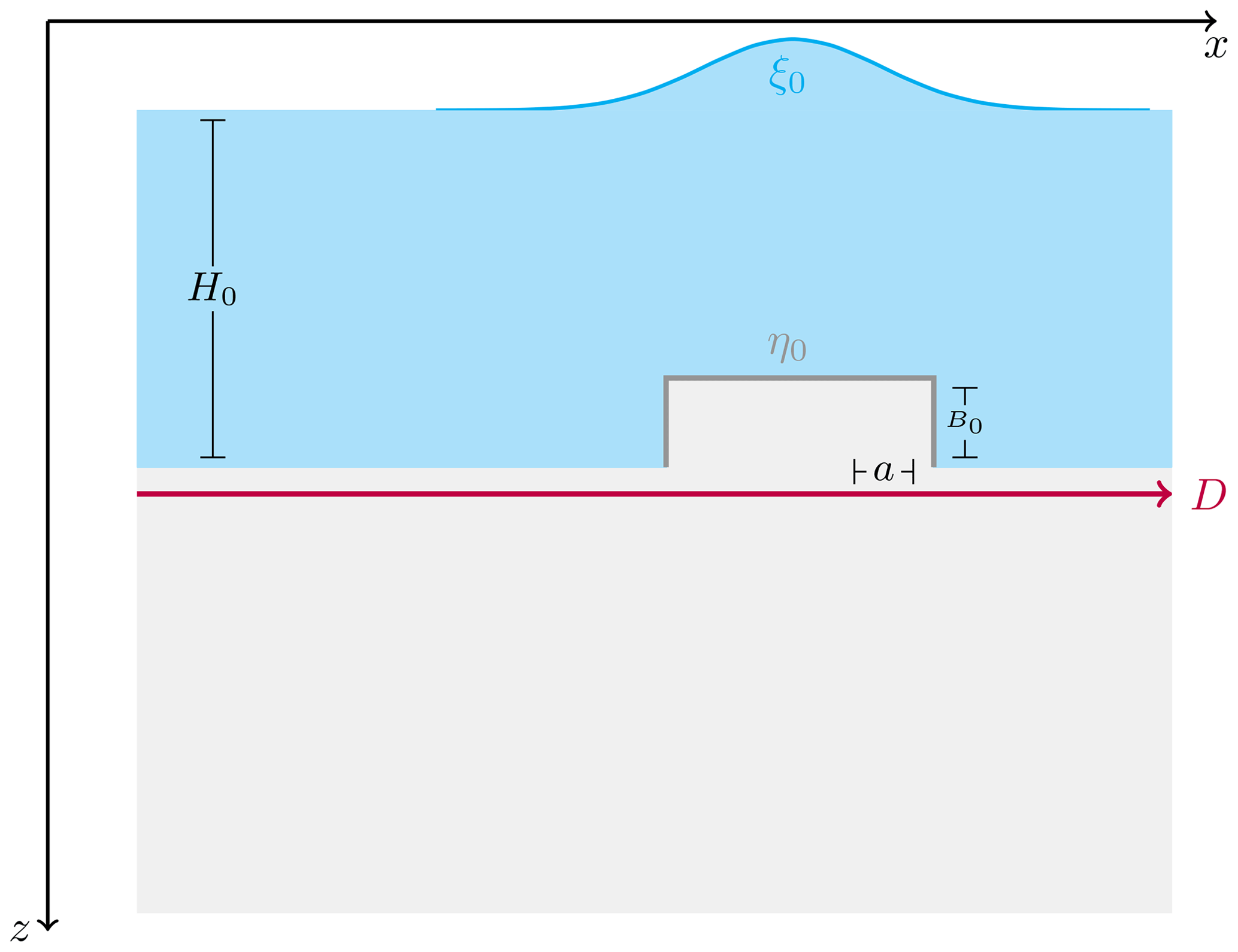
Figure 1 Schematic diagram of the problem in one dimension. The (flat) domain D is partitioned into cells of equal length a. In each cell, B₀ is the amplitude of the coseismic deformation η₀, modelled as the difference in two Heaviside functions. In the figure, only upward displacement in several adjacent cells with a constant water depth H₀ is sketched together with its effect ξ₀ at the sea surface. In reality, faulting would displace several cells either upward or downward in a more complex manner, and the water depth H₀ varies from place to place.

Formally, let R denote the set of real numbers. We consider a domain D⊂R, D being a track on the seafloor. D is partitioned into N_c sub-intervals $\mathit{\{}{c}_i{\mathit{\}}}_{i=\mathrm{1}}^{N_{\mathrm{c}}}$ of constant length a∈R, and x∈D is a point in this domain.

Within each cell c_i, the instantaneous uniform sea bottom displacement ${\mathit{\eta }}_{\mathrm{0}}^i$ is represented by a boxcar function obtained as the difference between the two Heaviside functions,

$$\begin{array}{}\text{(6)}& {\mathit{\eta }}_{\mathrm{0}}^i=B_{\mathrm{0}}^i\left[\mathit{\theta }(x+a)-\mathit{\theta }(x-a)\right],\end{array}$$

where $B_{\mathrm{0}}^i$ is the amplitude of ${\mathit{\eta }}_{\mathrm{0}}^i$. Equation (6) is used to exploit an analytical solution to Eq. (3). The corresponding sea surface height distribution (which we also call perturbation in the following) is given by Nosov and Sementsov (2014),

$$\begin{array}{}\text{(7)}& {\mathit{\xi }}_{\mathrm{0}}^i\left(x\right)={\displaystyle \frac{\mathrm{2}{B}_{\mathrm{0}}^i}{\mathit{\pi }}}\underset{\mathrm{0}}{\overset{\mathrm{\infty }}{\int }}{\displaystyle \frac{\cos \left(mx\right)\sin \left(ma\right)}{m\cosh \left(m{H}_{\mathrm{0}}^i\right)}}dm,\end{array}$$

where $H_{\mathrm{0}}^i$ the sea depth in c_i. Equation (7) is valid for flat bathymetry $H_{\mathrm{0}}^i$. However, Nosov and Sementsov (2014) also demonstrated its validity for arbitrary sloping bathymetry. The variable of integration m represents the spatial wavenumber and quantifies the number of oscillations of the integrand function in the domain of integration.

The term $F(k,H_{\mathrm{0}})=\frac{\mathrm{1}}{\cosh \left(m{H}_{\mathrm{0}}^i\right)}$ appearing in Eq. (7) is a Kajiura-type filter, which tends toward zero as $m{H}_{\mathrm{0}}^i\gg \mathrm{1}$, indicating that small wavelengths ($\mathit{\lambda }\ll H_{\mathrm{0}}^i$) are effectively attenuated. The free-surface perturbation ${\mathit{\xi }}_{\mathrm{0}}^i$ is also smooth, as it is derived analytically from the Laplacian problem (Eqs. 1–3). Each cell c_i is associated with what we will call, from now on, the local extended domain (LED),

$$\begin{array}{}\text{(8)}& l_{\mathrm{e}}^i=\left(-\mathrm{4}{H}_{\mathrm{0}}^i-{\displaystyle \frac{a}{\mathrm{2}}},\mathrm{4}{H}_{\mathrm{0}}^i+{\displaystyle \frac{a}{\mathrm{2}}}\right),\end{array}$$

whose extension depends on the sea depth. The initial condition given by Eq. (7) is solved numerically at every point $x_{\mathrm{p}}\in l_{\mathrm{e}}^i$. For all the points outside the LED (Eq. 8), the free-surface perturbation vanishes asymptotically (Nosov and Kolesov, 2011).

The unit initial conditions ${\mathit{\xi }}_{\mathrm{0}}^i$ generated by the bottom deformation within each segment c_i must later be combined to obtain the final sea surface perturbation (the tsunami initial condition) over the total domain D. In this section, we examine a unit cell c_i within the domain D, where the deformed seafloor (Eq. 6) perturbs the free surface as in Eq. (7). For simplicity, we temporarily exclude the superscript i when considering only one cell.

To solve the integral numerically, we follow these steps:

1. restrict the wavenumbers involved in the integration to a limited subset [0, U], where U is determined through tolerance tests for various parameterizations of the model (Eq. 7) and

2. identify the optimal quadrature method by comparing different solutions in terms of accuracy and computational efficiency.

More detailed information is provided in Sect. S1 of the Supplement.

3.1 Corner wavenumber for truncation

We seek to set the upper limit of the integration interval to a finite value of U, enabling us to solve the integration for a reduced subset of wave numbers only. Equation (7) can be restated as

$$\begin{array}{}\text{(9)}& \begin{array}{rl}{\mathit{\xi }}_{\mathrm{0}}\left(x\right)& ={\displaystyle \frac{\mathrm{2}{B}_{\mathrm{0}}}{\mathit{\pi }}}\left(a\mathit{ϵ}+O\left({\mathit{ϵ}}^{\mathrm{3}}\right)+\underset{\mathit{ϵ}}{\overset{U}{\int }}{\displaystyle \frac{\cos \left(mx\right)\sin \left(ma\right)}{m\cosh \left(m{H}_{\mathrm{0}}\right)}}dm\right.\\ & \left.+o\left(e^{-\frac{U{H}_{\mathrm{0}}}{\mathrm{2}}}\right)\right).\end{array}\end{array}$$

This is relevant to save computational time and to determine which wavelengths should be filtered out when transferring the sea bottom deformation to the sea surface level. We consider the cell size $s\in \mathit{\{}\mathrm{15},\mathrm{30},\mathrm{60}\mathit{\}}$, where the units are given in arc seconds (hereafter referred to as arcsec). This set of values is commonly adopted when modelling tsunamis. We then take a set of incremental discrete values for the local depth $d\in \mathit{\{}\mathrm{1},\mathrm{2},\mathrm{\dots },\mathrm{8}\mathrm{km}\mathit{\}}$. Each pair (s,d) is associated with an LED (Eq. 8) and with a free-surface height distribution $\widehat{{\mathit{\xi }}_{\mathrm{0}}^{s,d}}$ (Eq. 7).

Due to the product of a cosine and a sine oscillating at two distinct characteristic frequencies, the integrand function in Eq. (9) exhibits significant oscillations, calling for the use of an adaptive composite formula for its computation. The goal of a composite adaptive formula is to optimally partition the support into sub-intervals, whose number and length are dynamically selected by the algorithm. The sub-interval length decreases in those portions of the support domain where it is hard to get good accuracy and increases otherwise. Numerical integration is then executed in each sub-interval of the support, and the final result is obtained by summing the contributions of the solution within each sub-interval.

We employ a global adaptive quadrature (Shampine, 2008), hereafter identified by the acronym GAQ, as the reference solution for each of the 3×24 combinations of parameters s and d. The GAQ algorithm is a vectorized routine that automatically determines the number of sub-intervals for integral support based on user-defined absolute and relative tolerances, both set to 10⁻⁸ for our experiments. Given that the integral support in Eq. (7) is infinite, the GAQ algorithm performs an algebraic transformation to convert Eq. (7) into an equivalent integral on a finite interval, although this process is not visible to the user. To apply this transformation, the integrand must have weak singularities at the finite endpoint and decay rapidly at infinity. These conditions are verified in Sect. S1.1.

The truncation error $o\left(e^{-\frac{U{H}_{\mathrm{0}}}{\mathrm{2}}}\right)$ in Eq. (9) suggests that the upper limit U should be given in terms of the sea depth H₀ and in particular should be inversely proportional to it. Therefore, for each depth value d, we consider a range of possible upper limits, where each element is defined as $U_{j,d}=\frac{j}{d}$, with $j\in \mathit{\{}\mathrm{0.5},\mathrm{1},\mathrm{1.5},\mathrm{\dots },\mathrm{5}\mathit{\}}$. Each of the $\mathrm{3}\times \mathrm{24}\times \mathrm{10}$ combinations of cell size s, water depth d, and integral upper limit (UL) U_j,d is associated with a sea height distribution ${\mathit{\xi }}_{\mathrm{0}}^{s,j,d}$ according to Eq. (9), which is solved numerically, making use of GAQ as before within a truncated support [$\mathit{ϵ},U_{j,d}$]. For each j, the results of the truncated integration are compared to the reference solutions in terms of maximum absolute error (MAE),

$${\mathrm{MAE}}^{s,d,j}={\max }_x\mathrm{|}{\mathit{\xi }}_{\mathrm{0}}^{s,d,j}\left(x\right)-\widehat{{\mathit{\xi }}_{\mathrm{0}}^{s,d}\left(x\right)}\mathrm{|},$$

which sets the absolute tolerance when reconstructing the initial sea surface profile using limited subsets of wavenumbers.

The upper limit for the support of the integral in Eq. (9) can be defined depending on the desired tolerance level for a specific cell size. It can be seen from Fig. 2 that given U_j,d, tolerance generally increases when considering longer cells and shallower water, with some exceptions (see for instance the case corresponding to a cell size of 60 arcsec). However, for all the cell sizes and given a depth value, the tolerance decreases if U_j,d increases, as can be expected from the theoretical error. For all the combinations of parameters, the maximum tolerances are less than 50 cm and approach zero for $U_{j,d}\ge \frac{\mathrm{3}}{d}$. However, if the support of the integral contains few wavenumbers, the tails of its numerical solution may not be stable (see Sect. S1.1.1). To avoid this problem, we finally set the upper bound of the integral used in Eq. (9) as $U=\frac{\mathrm{5}}{H_{\mathrm{0}}}$ for all the possible values of H₀, which is aligned with the convergence condition requiring $U>\frac{\mathrm{2}}{H_{\mathrm{0}}}$. In particular, choosing $U=\frac{\mathrm{5}}{H_{\mathrm{0}}}$ gives a truncation error of $o\left(e^{-\frac{U{H}_{\mathrm{0}}}{\mathrm{2}}}\right)$ in Eq. (9) on the order of 0.5 %, which is considered sufficient for practical applications. The direct consequence is that all the wavelengths $\mathit{\lambda }<\frac{H_{\mathrm{0}}}{\mathrm{5}}$ will be filtered out in transferring seafloor deformation to the sea surface.

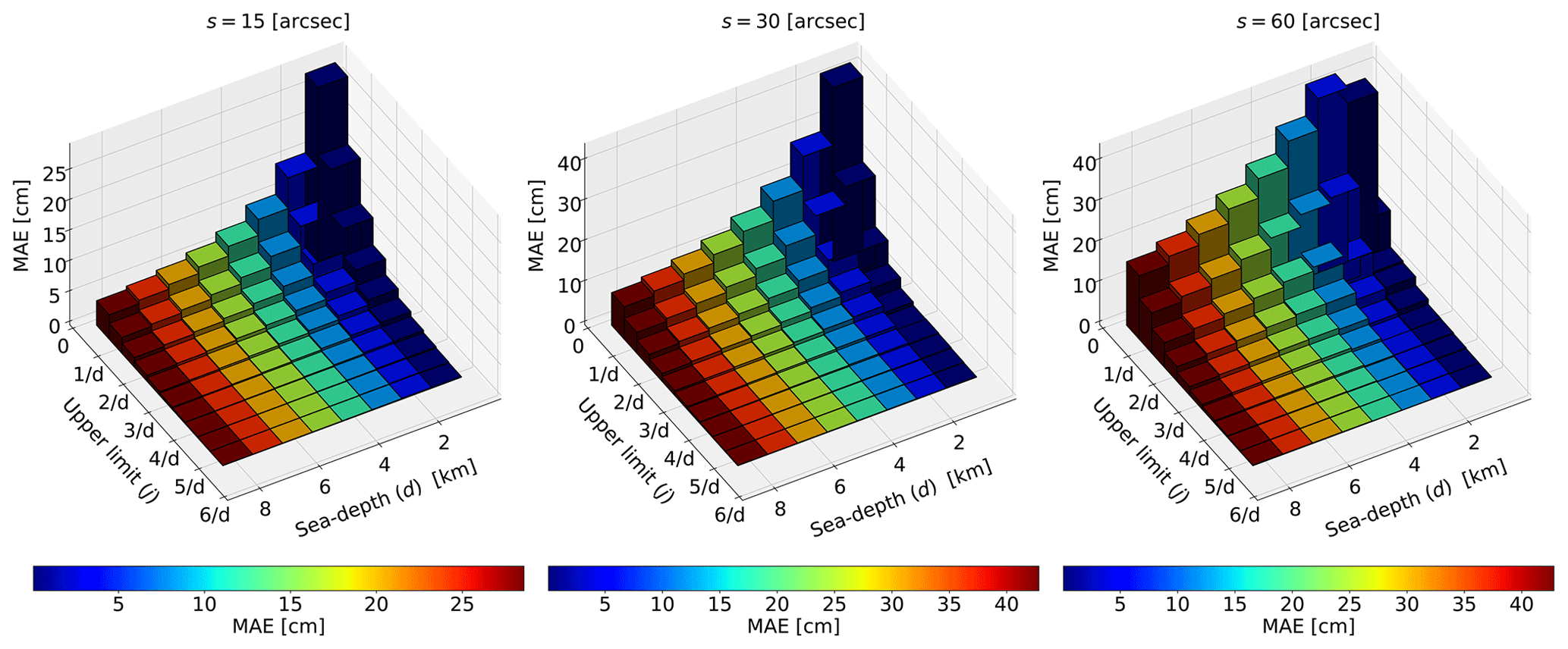
Figure 2 To identify the wavenumbers that play a substantial role in transferring seafloor deformation to the sea surface, we assess the tolerance by solving Eq. (9) with varying upper limits in the support of the integral. Additionally, we consider different model parameterizations, such as cell size and sea depth.

3.2 Optimal quadrature method for numerically solving the integral

In this section, we develop an adaptive scheme from scratch, optimized for handling the integrand function in Eq. (9). This involves automatically determining the number of sub-intervals for the integral support for the user and testing two different quadrature formulas to identify the most accurate and efficient one. While we introduce in this section two different quadrature formulae, we exploit the results discussed in the previous section: $U=\frac{\mathrm{5}}{H_{\mathrm{0}}}$, using the GAQ, and $\mathit{ϵ}={\mathrm{10}}^{-\mathrm{9}}$.

Since both the sine and cosine cannot be greater than one, Eq. (9) can be restated in a more convenient scaled version,

$$\begin{array}{}\text{(10)}& {\mathit{\xi }}_{\mathrm{0}}\left(x_{\mathrm{p}}\right)\simeq U{\displaystyle \frac{\mathrm{2}{B}_{\mathrm{0}}}{\mathit{\pi }}}\left({\displaystyle \frac{a\mathit{ϵ}}{U}}+\underset{m=\frac{\mathit{ϵ}}{U}}{\overset{\mathrm{1}}{\int }}{\displaystyle \frac{\cos \left(mU{x}_{\mathrm{p}}\right)\sin \left(mUa\right)}{mU\cosh \left(mU{H}_{\mathrm{0}}\right)}}dm\right),\end{array}$$

for each point x_p in the LED (Eq. 8) of the cell. It is important to emphasize that the integration domain $\left[\frac{\mathit{ϵ}}{U},\mathrm{1}\right]$ does not align with the spatial domain (Eq. 8). The former is associated with the wavenumber and expresses the physical wavelengths considered when modelling the sea surface after an instantaneous earthquake $\left[\frac{H_{\mathrm{0}}}{\mathrm{5}},{\mathrm{10}}^{\mathrm{9}}\right]$. The latter represents the discretization of the seafloor displacement into cells of equal length a. Equation (10) is an approximation of the seabed deformation transferred to the sea surface within a single cell, whose influence extends to all neighbouring cells within a distance of |4H₀| from the centre. In Eq. (10), the number of sub-partitions for the integral support should be determined based on the number of oscillations of the term $g(mU,x_{\mathrm{p}},a)=\cos \left(mUx\right)\sin \left(mUa\right)$ at the numerator of the integrand function. The function g is highly oscillatory because it is the product of a cosine and a sine, each oscillating at two distinct characteristic frequencies. Specifically, the individual frequencies are $w_{\mathrm{1}}=\frac{U{x}_p}{\mathrm{2}\mathit{\pi }}$ for the cosine and $w_{\mathrm{2}}=\frac{Ua}{\mathrm{2}\mathit{\pi }}$ for the sine, where x_p is the spatial point in the LED (Eq. 8) where the integral (Eq. 10) is evaluated, and a is the cell length. Therefore, the number (or frequency) of oscillations of g is controlled by the maximum between w₁ and w₂ and is defined by

$$\begin{array}{}\text{(11)}& w_{\max }=U\max \left({\displaystyle \frac{x_{\mathrm{p}}}{\mathrm{2}\mathit{\pi }}},{\displaystyle \frac{a}{\mathrm{2}\mathit{\pi }}}\right).\end{array}$$

According to the Nyquist theorem, the function g can be accurately reconstructed without any loss of information if it is sampled at a frequency that is at least twice the highest frequency of the function. Therefore, 2w_max, with w_max defined as in Eq. (11), gives the minimum number of sub-intervals for the support of the integral in Eq. (10). However, if w_max is too small, the resolution might not be enough to accurately describe some portions of the integration domain. To best represent the integrand in Eq. (10), the number of sub-intervals for the integral support is given by

$$\begin{array}{}\text{(12)}& N_m=\max \left[\mathrm{2}{w}_{\max },N_{\mathrm{s}}\right],\end{array}$$

where N_s is an integer that is sufficiently high to properly capture all the oscillations of g. This number was assessed by trial and error over a large number of different model parameterizations as N_s=10. At each point x_p in the LED (Eq. 8), Eq. (10) is solved within each of the N_m sub-intervals of the support $\left[\frac{\mathit{ϵ}}{U},\mathrm{1}\right]$. The value of the free-surface perturbation at x_p is found by aggregating the individual results from a quadrature formula within each sub-interval. Two different quadrature methods are compared here.

1. The Gauss–Legendre quadrature with three points (justified by the harmonic nature of the analytical solution to the problem, Eq. 10), hereafter called GLQ (Sect. S2.1).

2. The Filon-type quadrature, which is well known to be efficient in cases of highly oscillating integrands (Filon, 1930; Iserles, 2004). We will refer to it as FQ (Sect. S2.2).

The deformed free-surface ξ₀ is found for three different cell sizes (15, 30, and 60 arcsec) and for eight depth values, ranging from 1 to 8 km every 1 km. Results are checked against the reference solution (GAQ) as in Sect. 3.1. We compare the algorithms in terms of their efficiency (execution time) and accuracy. The efficiency is measured considering the average execution time of three runs. The accuracy is provided as the root-mean-square error (RMSE) averaged over all the sea depths considered.

We find that the RMSEs between the various numerical solutions are comparable: $\mathrm{3.45}\times {\mathrm{10}}^{-\mathrm{4}}$ for 15 arcsec, $\mathrm{4.81}\times {\mathrm{10}}^{-\mathrm{4}}$ for 30 arcsec and $\mathrm{4.64}\times {\mathrm{10}}^{-\mathrm{4}}$ for 60 arcsec. The practical difference between the two algorithms lies in the execution time, which is roughly 1 order of magnitude faster for GLQ than for the adapted FQ (Fig. 3). For comparison, the execution time for GAQ is 0.319 s for 15 arcsec, 0.331 s for 30 arcsec, and 0.357 s for 60 arcsec, which is slightly less than FQ and about 1 order of magnitude more than GLQ. Note, however, that the GAQ and Filon routines used here are the MATLAB ones; hence, they are probably already more optimized than the GLQ routine we developed. Our preferred solver is thus the GLQ.

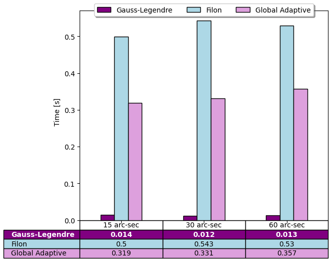
Figure 3 The efficiency of the different adaptive quadrature formulae, Gauss–Legendre (GLQ), Filon (FQ), and global adaptive (GAQ), is illustrated in the histograms. For each cell size, the computation time, averaged across the eight depth values, is shown.

4 The 2D case

The integration limit U and the optimal quadrature method (GLQ) for the 2D case are chosen based on the tests for one dimension. In Sect. 3.2, we establish that this algorithm is the most efficient for accurately approximating the deformation of the free surface. These results can be extended to the 2D case due to symmetry.

In 2D, the domain D⊂R² is discretized into a finite number $N_{\mathrm{c}}^x\times N_{\mathrm{c}}^y$ of cells {c_ij} having the constant area a×b, with a as the extension along $\widehat{x}$, and b as the one along $\widehat{y}$. The subscripts i and j refer to the nodes in the grid along $\widehat{x}$ and $\widehat{y}$, respectively. The pair of coordinates $(x,y)\in D$ is a point in the domain. Within each cell c_ij, the instantaneous uniform bottom displacement is again modelled as the difference between two Heaviside functions (Nosov and Kolesov, 2011) as

$$\begin{array}{}\text{(13)}& {\mathit{\eta }}_{\mathrm{0}}^{ij}(x,y)=B_{\mathrm{0}}^{ij}\left[\mathit{\theta }\right(x+a)-\mathit{\theta }(x-a\left)\right]\left[\mathit{\theta }\right(y+b)-\mathit{\theta }(y-b\left)\right].\end{array}$$

The sea surface perturbation given by Eq. (16) in Nosov and Kolesov (2011) can be restated directly as

$$\begin{array}{}\text{(14)}& \begin{array}{rl}{\mathit{\xi }}_{\mathrm{0}}^{ij}& (x,y)\simeq U^{\mathrm{2}}{\displaystyle \frac{\mathrm{4}{B}_{\mathrm{0}}^{ij}}{{\mathit{\pi }}^{\mathrm{2}}}}\left({\displaystyle \frac{ab\mathit{ϵ}}{U^{\mathrm{2}}}}+O\left({\mathit{ϵ}}^{\mathrm{4}}\right)\right.\\ & \left.+\underset{\frac{\mathit{ϵ}}{U}}{\overset{\mathrm{1}}{\int }}\underset{\frac{\mathit{ϵ}}{U}}{\overset{\mathrm{1}}{\int }}{\displaystyle \frac{\cos \left(Umx\right)\sin \left(Uma\right)\cos \left(Uny\right)\sin \left(Unb\right)}{mn{U}^{\mathrm{2}}\cosh \left(kU{H}_{\mathrm{0}}^{ij}\right)}}dmdn\right),\end{array}\end{array}$$

where $B_{\mathrm{0}}^{ij}$ is the residual bottom deformation and $H_{\mathrm{0}}^{ij}$ is the water depth, taken as positive downward, in the cell c_ij. The variables of integration m and n represent the spatial wave numbers along $\widehat{x}$ and $\widehat{y}$, respectively. The variable $k=\sqrt{m^{\mathrm{2}}+n^{\mathrm{2}}}$ is the modulus of the wave vector. The values of $\mathit{ϵ}={\mathrm{10}}^{-\mathrm{9}}$ and $U=\frac{\mathrm{5}}{H_{\mathrm{0}}^{ij}}$ are set according to the analysis presented in Sect. 3.1. In two dimensions, the LED is defined by a rectangular area surrounding the cell (Fig. 4) in the Cartesian plane,

$$\begin{array}{}\text{(15)}& {\displaystyle }& {\displaystyle }{p}_{\min }=-\mathrm{4}{H}_{\mathrm{0}}^{ij}-\max \left({\displaystyle \frac{a}{\mathrm{2}}},{\displaystyle \frac{b}{\mathrm{2}}}\right),\text{(16)}& {\displaystyle }& {\displaystyle }{p}_{\max }=\mathrm{4}{H}_{\mathrm{0}}^{ij}+\max \left({\displaystyle \frac{a}{\mathrm{2}}},{\displaystyle \frac{b}{\mathrm{2}}}\right),\text{(17)}& {\displaystyle }& {\displaystyle }{l}_{\mathrm{e}}^x=p_{\min },p_{\min }+\mathrm{\Delta }x,p_{\min }+\mathrm{2}\mathrm{\Delta }x,\mathrm{\dots },p_{\max }-\mathrm{\Delta }x,p_{\max },\text{(18)}& {\displaystyle }& {\displaystyle }{l}_{\mathrm{e}}^y=p_{\min },p_{\min }+\mathrm{\Delta }y,p_{\min }+\mathrm{2}\mathrm{\Delta }y,\mathrm{\dots },p_{\max }-\mathrm{\Delta }y,p_{\max }.\end{array}$$

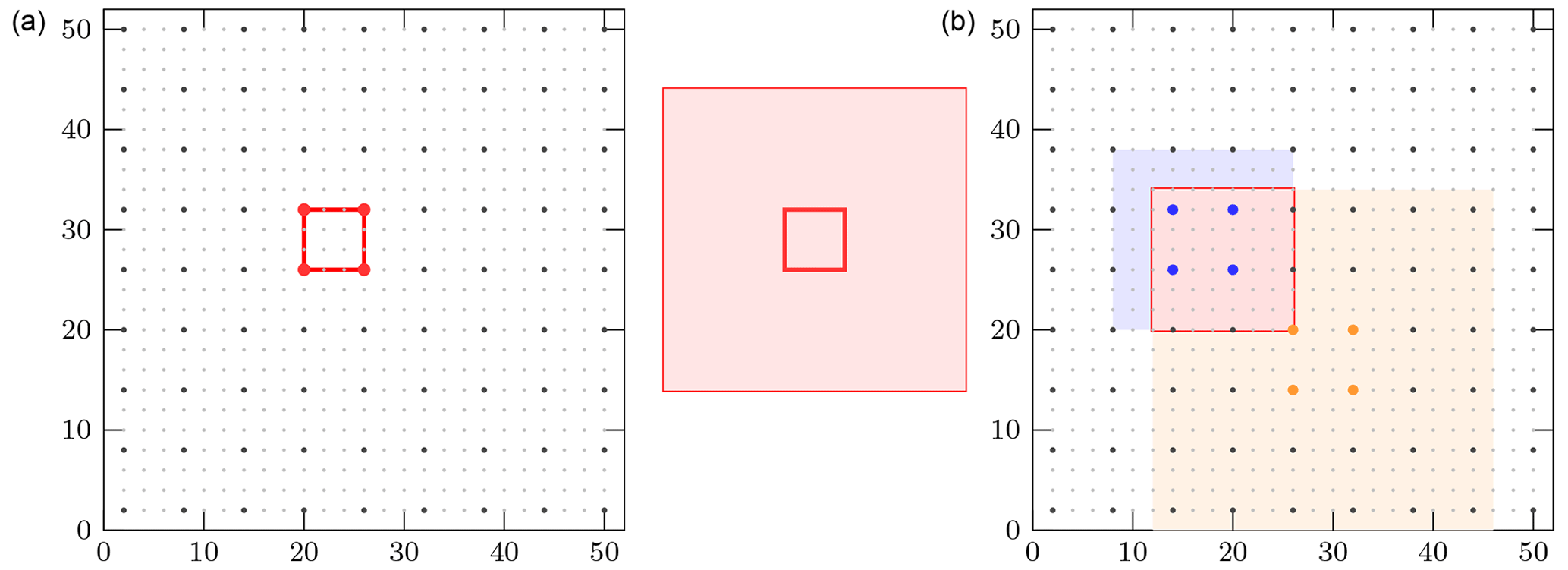
Figure 4 (a) A single cell is shown, together with the associated LED. The depth of the water is 3 km, to scale. (b) Two cells and their associated LEDs are shown. The sea depths are, to scale, 1.5 km for the blue cell and 3 km for the orange cell. The unit contributions to the total perturbation of the free surface will be superimposed at the intersection of the two LEDs.

Numerical solutions for Eq. (14) are computed at each point (x_p,y_p) within Eq. (15), using GLQ with four points. The numerical scheme for its extension to the 2D case can be found in the Supplement.

4.1 Physical interpretation

Two experiments detailed in Fig. 5 are conducted in both 1D and 2D. The amplitude of the sea floor deformation is kept constant at B₀=1 m in both cases. In the 1D scenario, H₀ is initially set to 4 km, with varying cell sizes of 450, 900, and 1800 m (approximately 15, 30, and 60 arcsec, respectively). We then explore the case where the Heaviside function (Eq. 6) encompasses typical wavelengths of coseismic deformation. To establish reasonable orders of magnitude, these wavelengths are set as equivalent to a=wcos (δ), representing the projection of a fault width w onto the horizontal plane through the dip angle δ. Specifically, we consider a dip of δ=15° for a fault plane having a width of w=11 km and $\mathit{\delta }\in \mathit{\{}\mathrm{20},\mathrm{45}\mathit{°}\mathit{\}}$ for the one with w=27 km, roughly corresponding to moment magnitudes of M_w=6 and M_w=7, according to the scaling relations presented in Strasser et al. (2010). The initial sea surface height is evaluated through Eq. (10) for each cell length. Figure 5a shows that the smoothing effect increases as the source size decreases, leading to a progressively lower amplitude and narrower width. Sources whose extents are much shorter than the sea depth (15 arcsec, 30 arcsec, and 60 arcmin) are unable to efficiently lift the water column up. Doubling the source size relative to the sea depth, as in the case of a≃11 km, results in an elevation essentially reproducing the unfiltered bottom deformation at the surface, with a maximum of +0.98 m. If the source length is more than 4 times the local water depth, which is the case of a≃19 and a≃27 km, the maximum crest of the water height matches that at the sea bottom, and filtering affects only the corner of the boxcar. The experiment is replicated for the 2D case, where the values for a are equivalent to those employed in the 1D scenario, and b is set at half of the corresponding a values. In Fig. 5b, a segment of the free-surface disturbance along the $\widehat{x}$ axis is depicted, corresponding to the blue line in the top panel of Fig. 5. Simultaneously, Fig. 5c illustrates the profiles acquired along the $\widehat{y}$ axis, mirroring the scenario of the magenta plane. The behaviour of the model (Eq. 14) aligns with the 1D scenarios for the tested source sizes: a broader extension of the Heaviside function describing coseismic deformation (Eq. 13) results in a less-pronounced smoothing effect on the free-surface deformation. Nevertheless, in the 2D case, the maximum free-surface elevation values obtained are slightly lower than those in the 1D case: +0.01 m for a=450 m and b=225 m, +0.03 m for a=900 m and b=450 m, +0.1 m for a=1800 m and b=900 m, +0.83 m for a≃11 and b≃5 km, +0.97 m for a≃19 and b≃10 km and +0.99 m for a≃26 and b≃13 km. Figure 5d illustrates the scenario where the 1D unit source length is held constant at $a=\simeq \mathrm{11}$ km as before, with varying depths of 1, 4, and 8 km, respectively, corresponding to the average depths of the Mediterranean Sea, the Pacific Ocean, and trench axes in subduction zones. As the sea depth increases, the sea surface uplift diminishes, accompanied by an expansion in the width of the water height distribution. For H₀=1 km, the bottom deformation is almost perfectly replicated on the surface in both shape and elevation. With H₀=4 km, the uplift reaches a maximum of +0.98 m, and the deformation shape is smoothed. When the sea depth is 8 km, the peak is +0.84 m, and the elevation is redistributed over the tails. A similar trend is observed in Fig. 5e and f, representing two sections of a 2D free-surface perturbation along the $\widehat{x}$ and $\widehat{y}$ axes, respectively. For H₀=1 km, results align with the 1D case. The maximum crest is reduced to +0.83 m for H₀=4 km and to +0.5 m for H₀=8 km, indicating that the lateral extension of the coseismic deformation plays a crucial role with varying sea depths. The findings indicate that the damping level of the 2D filter is closely related to the ratio of wavelengths in the $\widehat{x}$ and $\widehat{y}$ directions. Specifically, the shorter the deformation in one direction, the more pronounced the smoothing in the other direction. In the Supplement, we provide a comparison between the scenarios presented in this section and the outcomes derived from the application of a Kajiura-type filter with different parameterizations of the coseismic deformation and sea depth values. Additionally, we present the 2D shapes of the free-surface perturbations corresponding to the 1D sections depicted in Fig. 5b, c, e, and f.

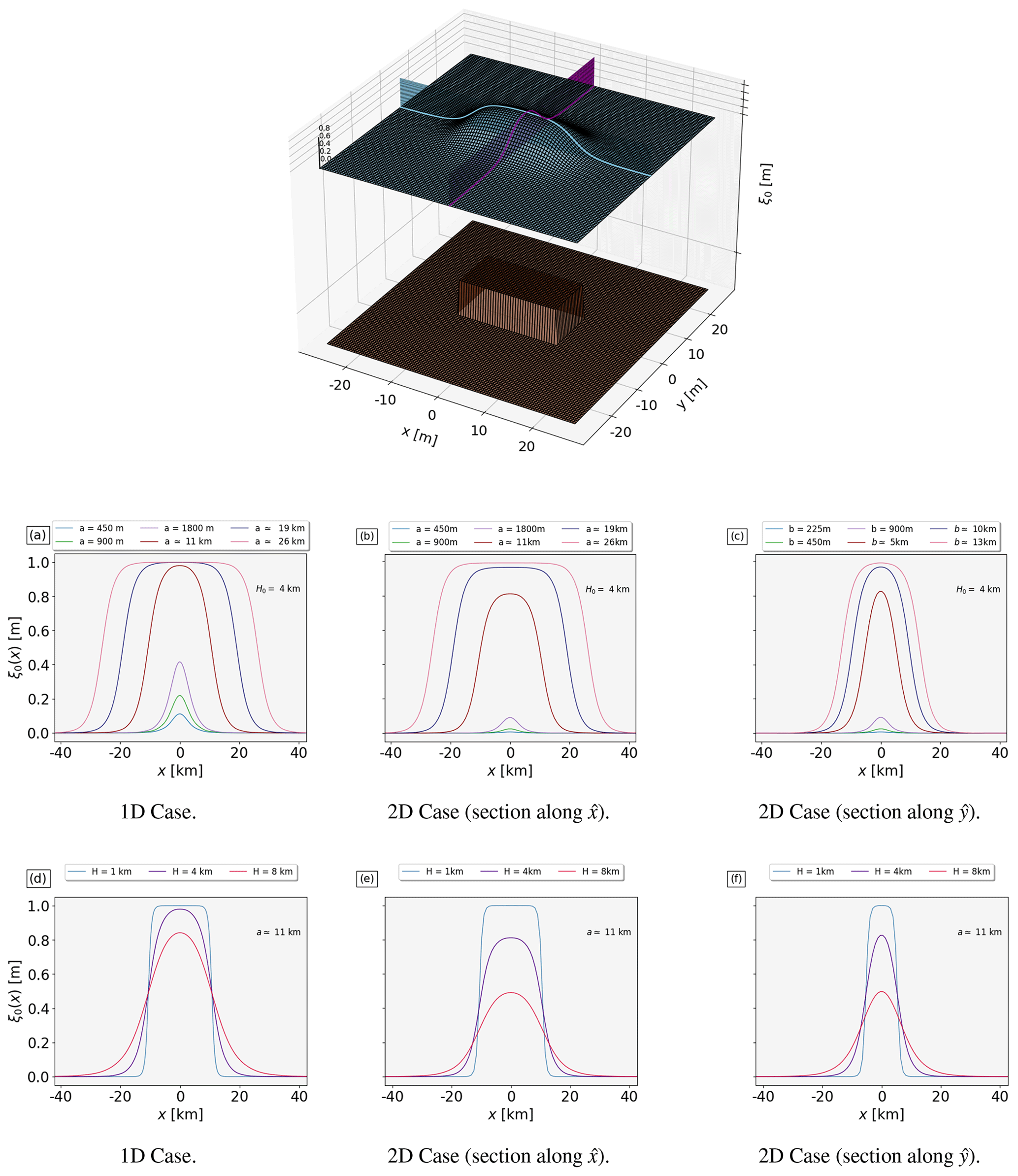
Figure 5 The problem in two dimensions is illustrated in the upper panel. The coseismic deformation η₀ is modelled as described in Eq. (13), given a length a, a width b, and an amplitude B₀=1 m. This deformation leads to the uplift of the sea surface, causing the perturbation ξ₀. Panels (a) and (d) show the 1D perturbations of the free surface obtained by solving Eq. (10), considering a constant sea depth and a constant cell length, respectively. Panels (b), (c), (e), and (f) show profiles extracted from equivalent 2D cases, evaluated through Eq. (14) along the two perpendicular planes shown in the top panel.

4.2 How to construct a local database of unit-smoothed initial conditions for tsunami propagation

The mathematical model proposed by Nosov and Kolesov (2011) along with its equivalent scaled version presented in Eq. (14), is fully characterized by three parameters: sizes a and b of the rectangular cells by which the domain under study has been discretized and the water depth $H_{\mathrm{0}}^{ij}$ within each cell c_ij. We note that the amplitude $B_{\mathrm{0}}^{ij}$ of the bottom deformation (Eq. 13) serves in Eq. (14) as a multiplicative constant outside the integral. This observation suggests that Eq. (14) can be independently solved for each c_ij∈D. Individual solutions can be derived depending solely on the water depth $H_{\mathrm{0}}^{ij}$ inside the cell and the linear dimensions a, b of the cell itself. Without a loss of generality, we can set $B_{\mathrm{0}}^{ij}=\mathrm{1}$ within each cell.

The results, each representing a scaled and filtered free-surface deformation, can be stored in a repository to be used as a database of unit sources that can be linearly combined to approximate the tsunami initial condition due to any sea bottom deformation (Fig. 4). Assuming sea depth is constant within a cell, Eq. (14) is an analytical solution to the Laplace problem in Eqs. (1)–(4) for the scalar potential of fluid displacement. Since the Laplace operator is linear, the superposition principle allows us to linearly combine elementary contributions. We design an algorithm, from now on identified by the acronym LST (Laplacian smoothing tool).

Pseudo-code of the LST algorithm along with its 1D version are provided in the Supplement. The LST Bash and Python scripts are also provided (see “Code and data availability” section).

5 Test on real events

5.1 The tsunamigenic earthquakes in the central Kuril Islands

In late 2006 and early 2007, two large earthquakes occurred near the Kuril Trench (Fig. 6). Both the events triggered tsunami waves that spread across the Pacific Ocean and were detected by numerous Deep-ocean Assessment and Reporting of Tsunamis (DART) buoys, tide gauges, and bottom-pressure sensors in the far field. There were no coastal stations in the near field, with the nearest located at least 500 km away from the source (Fujii and Satake, 2008; Rabinovich et al., 2008; Tanioka et al., 2008; Nosov and Kolesov, 2009, 2011). The 15 November 2006 earthquake had a moment magnitude of 8.3 (CMT; https://www.globalcmt.org/cgi-bin/globalcmt-cgi-bin/CMT5/form?itype=ymd&yr=2006&mo=11&day=15&oyr=2006&omo=11&oday=15&jyr=1976&jday=1&ojyr=1976&ojday=1&otype=nd&nday=1&lmw=8.3&umw=8.3&lms=0&ums=10&lmb=0&umb=10&llat=-90&ulat=90&llon=-180&ulon=180&lhd=0&uhd=1000&lts=-9999&uts=9999&lpe1=0&upe1=90&lpe2=0&upe2=90&list=0, last access: 17 August 2024), and its hypocentre was located at the interface between the subducting Pacific and the Okhotsk plates, at 46.592° N, 153.266° E (USGS; https://earthquake.usgs.gov/earthquakes/map/?currentFeatureId=usp000f2ab&extent=-89.51899,-382.5&extent=89.51305,742.5&range=search&timeZone=utc&search={"name":"SearchResults","params":{"starttime":"2006-11-1500:00:00","endtime":"2006-11-1523:59:59","minmagnitude":8.3,"maxmagnitude":8.3,"orderby":"time"}}, last access: 17 August 2024). A second earthquake followed approximately 2 months later, on 13 January 2007. The earthquake was an outer rise with a normal fault mechanism. The CMT algorithm (https://www.globalcmt.org/cgi-bin/globalcmt-cgi-bin/CMT5/form?itype=ymd&yr=2007&mo=01&day=13&oyr=2007&omo=01&oday=13&jyr=1976&jday=1&ojyr=1976&ojday=1&otype=nd&nday=1&lmw=8.1&umw=8.1&lms=0&ums=10&lmb=0&umb=10&llat=-90&ulat=90&llon=-180&ulon=180&lhd=0&uhd=1000&lts=-9999&uts=9999&lpe1=0&upe1=90&lpe2=0&upe2=90&list=0 last access: 17 August 2024) estimated a moment magnitude of M_w=8.1. The hypocentre was situated along a high-angle fault beneath the trench slope, at 46.243° N, 154.524° E (USGS; https://earthquake.usgs.gov/earthquakes/map/?currentFeatureId=usp000f2ab&extent=-89.61433,-382.5&extent=89.60957,742.5&range=search&timeZone=utc&search={"name":"Search Results","params":{"starttime":"2007-01-13 00:00:00","endtime":"2007-01-13 23:59:59","minmagnitude":8.1,"maxmagnitude":8.1,"orderby":"time"}}, last access: 21 August 2024).

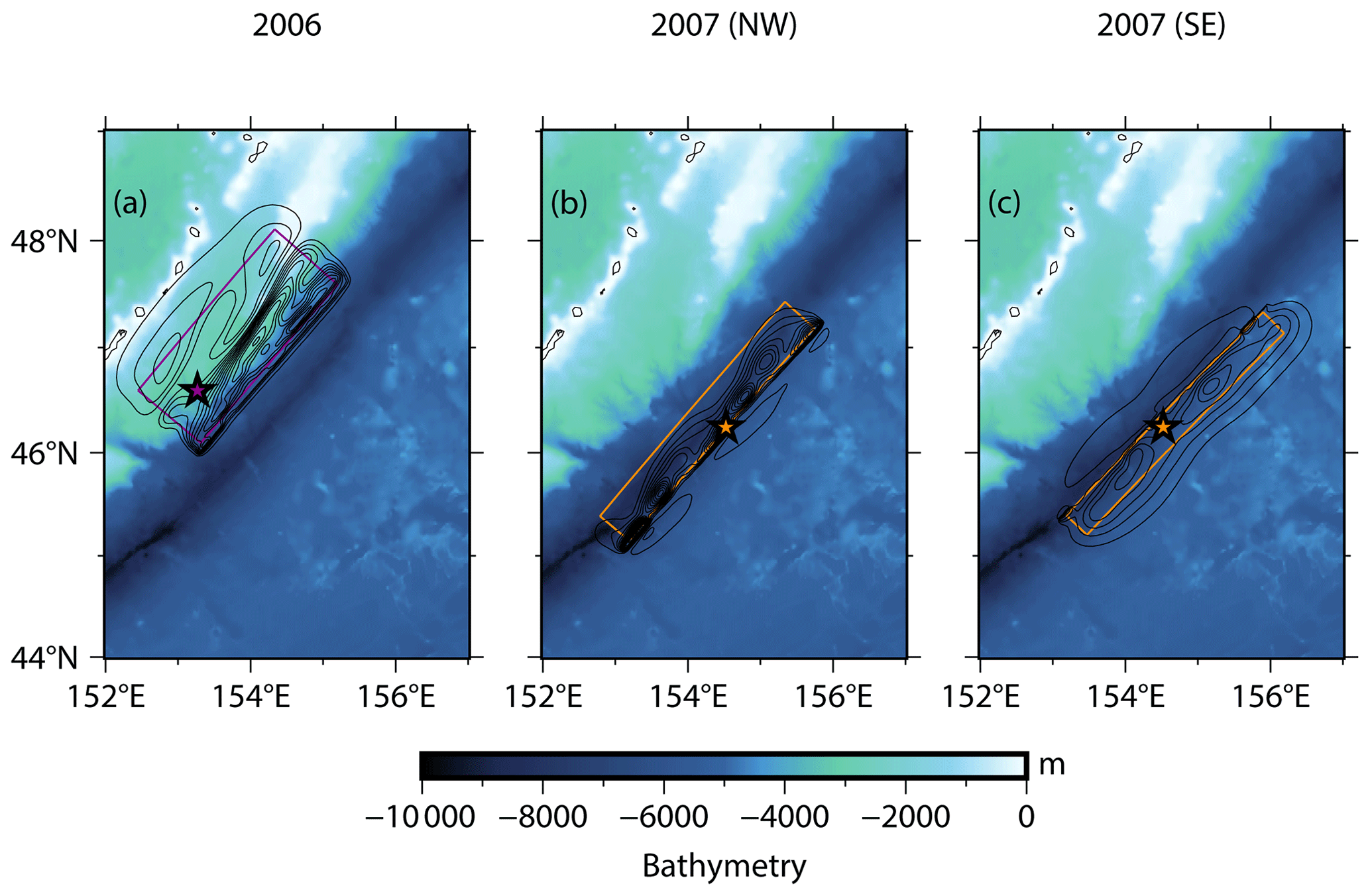
Figure 6 The fault planes (Lay et al., 2009) and contour lines depicting vertical coseismic deformations (with a 0.25 m interval) for seismic events in the central Kuril Islands during late 2006 and early 2007. These deformations are calculated using the Okada (1985) algorithm. Panel (a) refers to the megathrust event (late 2006). In the case of the outer-rise event (early 2007), two distinct slip models are taken into account, as shown in panels (b) and (c). Additionally, the epicentres of the earthquakes, sourced from the USGS catalogue, are marked for reference.

We consider here the slip distributions on planar faults published in Lay et al. (2009) for both events (Fig. 6). The slip model for the 2006 event is based on the inversion of teleseismic P waves. The slip model for the 2007 event relies on the inversion of teleseismic P and SH waves. Two different potential fault plane orientations have been identified, one northwest dipping and the other southeast dipping. The data did not allow us to conclusively determine a preferred plane, leading to the consideration of both orientations. According to Lay et al. (2009), the 2006 event ruptured at a very shallow depth. As for the 2007 event, the exact position of the slip in relation to the bathymetry is uncertain. However, for both events, there is no evidence that the rupture reached the seafloor.

For the three slip models, we compute the 3D coseismic deformation resulting from each sub-fault in which the fault plane is partitioned as a vector ${\mathit{\eta }}_{\mathrm{0}}=({\mathit{\eta }}_{\mathrm{0}x},{\mathit{\eta }}_{\mathrm{0}y},{\mathit{\eta }}_{\mathrm{0}z})$, where η_0x and η_0y denote deformations in the horizontal directions, modelled as in Eq. (13), while η_0z represents the vertical component. Subsequently, these individual contributions are aggregated to form the total seafloor deformation.

For all the three fault plane geometries, we consider two different models to test the LST algorithm.

The first one is η_0z, obtained by combining the vertical components of the coseismic deformation produced by each sub-fault (Fig. 6). The second one, ${\mathit{\eta }}_{\mathrm{0}z}+{\mathit{\eta }}_{\mathrm{0}x}\frac{\partial H_{\mathrm{0}}}{\mathrm{d}x}+{\mathit{\eta }}_{\mathrm{0}y}\frac{\partial H_{\mathrm{0}}}{\mathrm{d}y}$, accounts for the impact of the horizontal movement of a sloping bottom combined with the vertical component. The horizontal movement, particularly on steep slopes such as that of the Kuril Trench, has been identified as a significant factor in generating seismotectonic tsunamis (Iwasaki, 1982; Tanioka and Satake, 1996; Tanioka and Seno, 2001). Following the notation in Tanioka and Seno (2001), the latter is identified hereafter as Model A and is equivalent to Eq. (2) in Tanioka and Satake (1996).

We also consider Model B proposed in Tanioka and Seno (2001) but only for the 2006 megathrust event, which is a proxy for the inelastic dislocation of the sediments within the accretionary wedge due to the movement of the corresponding backstop. This model is given by ${\mathit{\eta }}_{\mathrm{0}z}+\left({\mathit{\eta }}_{\mathrm{0}x}\frac{\partial H_{\mathrm{0}}}{\mathrm{d}x}+{\mathit{\eta }}_{\mathrm{0}y}\frac{\partial H_{\mathrm{0}}}{\mathrm{d}y}\right)\frac{h}{w}$, with h and w representing the height of the backstop and the width of the sediments in the wedge, respectively. For Model B, specific values are chosen, such as h=8 km and w=20 km, which are to be taken as orders of magnitude derived from the structural and tectonic sections presented in Qiu and Barbot (2022).

A single database of smoothed unit sources, spanning from 44 to 49° N in latitude and from 152 to 157° E in longitude, is constructed and encompasses 300×299 smoothed source elevation values, as detailed in Sect. 4. For this application, we use the bathymetry model SRTM30+ (Becker et al., 2009) downsampled at 1 arcmin.

The results for the 2006 event are illustrated in Fig. 7. The sea bottom deformation induced by the vertical component (Fig. 6a) spans from a maximum subsidence of −0.81 m to a maximum uplift of +2.80 m (Fig. 7a).

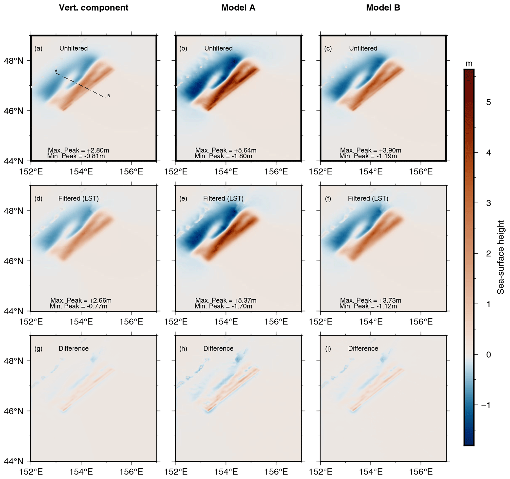
Figure 7 Results for the tsunamigenic earthquake that occurred on 15 November 2006. Panels (a), (d) and (g) depict the sea surface distribution arising from vertical bottom movement. The last two columns present the results obtained with the contribution of the horizontal displacement according to Tanioka and Seno (2001). In particular, panels (b), (e), and (h) refer to Model A, while panels (c), (f), and (i) refer to Model B. Panel (a) depicts the transect AB where 1D profiles for all six models have been considered. Panels (g)–(i) show how the simple differences between the unfiltered and filtered initial conditions are spatially distributed.

The output from LST yields an elevation of +2.66 m and a subsidence of −0.77 m (Fig. 7d). The magnitudes are, in modulus, slightly higher than those reported by Nosov and Kolesov (2011) (+2.55 m upwelling and −0.58 m downwelling) but significantly higher than the results obtained by Rabinovich et al. (2008) using a 3D implementation of the Laplace problem for the same case (+1.9 m uplift). These discrepancies in the final water height may be attributed to the different slip and bathymetric models used. The horizontal component substantially displaces the seafloor. In the unfiltered version of Model A, a peak elevation of +5.64 m and a downwelling of −1.80 m are observed in the deformation field (Fig. 7b). The application of LST results in a maximum upward movement of +5.37 m and a minimum downfall of −1.70 m (Fig. 7e). The deformation computed through Model B shows a systematically lower maximum crest than in Model A. In projecting the horizontal deformation onto the vertical plane, the deformation extent in Model B is regulated by the ratio between the backstop height (h) and the width of the accretionary wedge (w), expressed as $\frac{h}{w}$. Depending on the relative values of the two parameters, particularly when w is significantly higher than h as in this case, this ratio may lead to a damping effect on the contribution from the horizontal component of deformation. The maximum unfiltered uplift for Model B amounts to +3.90 m, lowered to +3.73 m by LST, while the maximum unfiltered depression measures −1.19 m, reduced to −1.12 m when our algorithm is applied (Fig. 7c and f). The last row of Fig. 7 depicts the spatial distributions of differences between the unfiltered and the filtered sea surface height for all three models considered. Major differences in uplift and subsidence are observed in deep waters towards the trench, consistent with the synthetic cases shown in Fig. 5. The sea depth in the area of interest related to the high wavenumber damping ranges from 3 to 7 km, as can be seen in Fig. 6. Another insight is provided by Fig. 8, which shows the 1D profiles along the transect AB depicted in Fig. 7a for all nine models. However, it is interesting to note that all three unfiltered profiles (resulting from the vertical-only coseismic deformation, Model A, and Model B) exhibit three distinct peaks that are smoothed by the filtering process, resulting in a single pronounced peak.

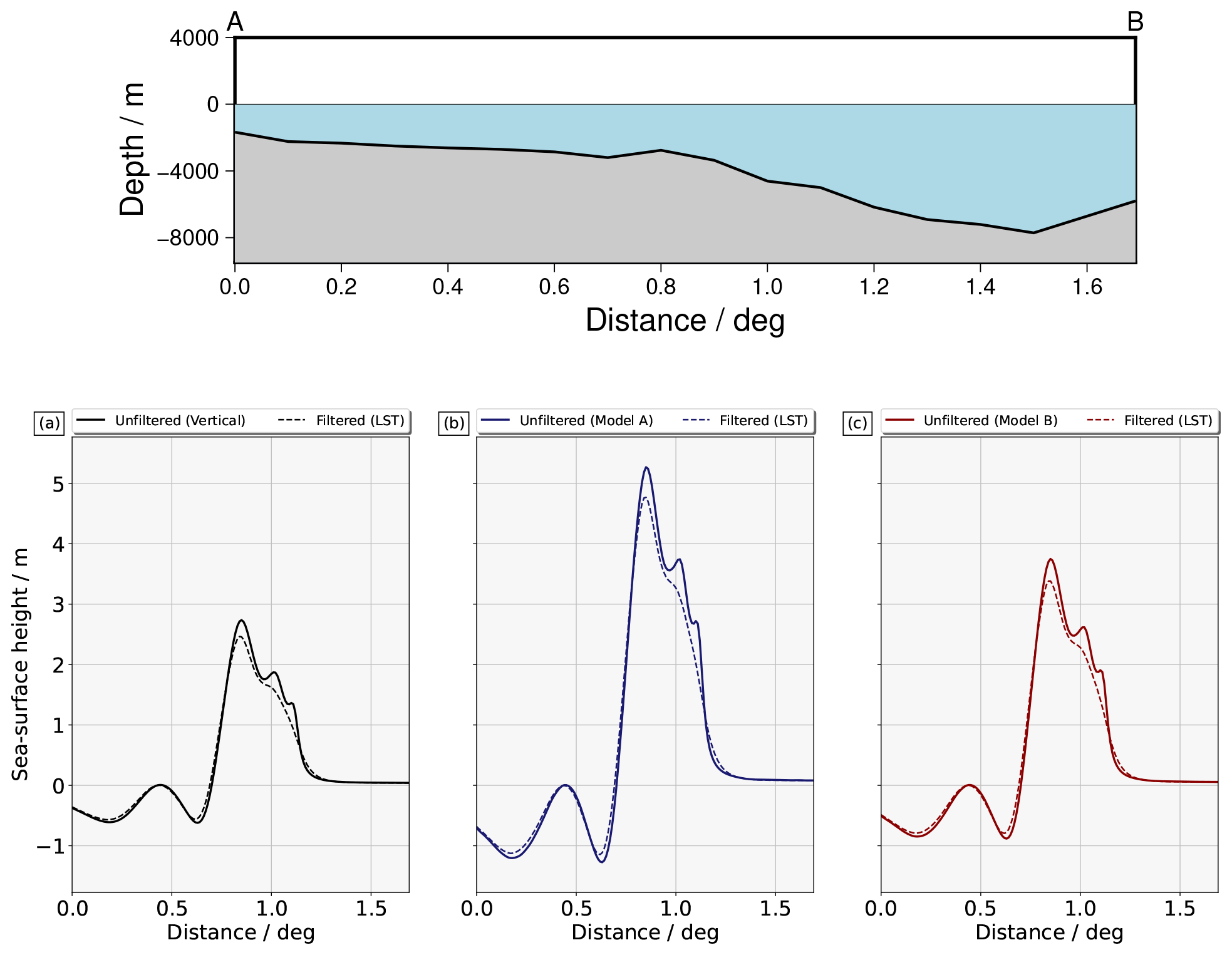
Figure 8 The transect AB under consideration is depicted in Fig. 7a. The upper panel illustrates the bathymetric profile. In (a), the profiles are derived from the initial conditions shown in Fig. 7a, d, and g, taking into account only the vertical component. In (b), the profiles are obtained from the initial conditions in Fig. 7d, e, and h, incorporating the influence of the horizontal component through Model A. Lastly, in (c), the profiles are extracted from the initial conditions in Fig. 7c, f, and i, considering the effect of the horizontal component through Model B.

For the 2007 event, we use only the vertical component (Fig. 6b and c) and Model A (vertical and projection of the horizontal), as the earthquake occurred in the oceanic crust relatively far from the sedimentary wedge. The outcomes for the northwest dipping fault plane are depicted in Figs. 9 and 10. The sea surface perturbation resulting from the vertical component of the seafloor deformation exhibits a maximum of +0.57 m and a minimum of −5.06 m (Fig. 9a). The application of our LST algorithm yields a positive elevation of +0.29 m and a negative peak of −2.42 m (Fig. 9c), which is less than half the value obtained by translating the seabed deformation to the surface. The filtering effects become more pronounced when considering all 3D components of displacement with Model A, reducing the maximum uplift from +1.13 to +0.56 m and increasing the maximum depression from −10.15 to −4.86 m (Fig. 9b and d). The northwest-oriented fault plane, as adopted by Nosov and Kolesov (2011) with a different slip distribution, results in different numerical values, but their application of the Laplace smoothing algorithm produces almost identical results to those of the LST one, consistently halving the maximum trough. We show the spatial differences between the unfiltered and the filtered sea surface perturbation in the last row of Fig. 9. As for the 2006 case, the smoothing is focused along the trench and is more pronounced in the proximity of the deepest zones (see Fig. 10 and Fig. 6 for comparison).

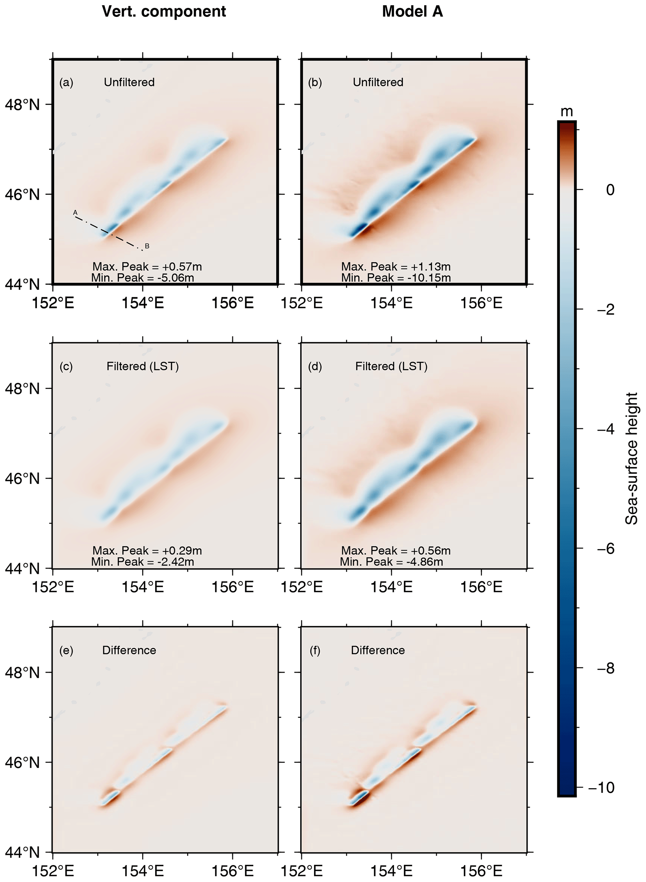
Figure 9 Results for the tsunamigenic earthquake that occurred on 13 January 2007. The fault plane is northwest dipping. Panel (a) depicts the transect AB where 1D profiles for all models have been considered. Panels (a), (c), and (e) present a sea surface perturbed by a vertical bottom deformation. Panels (b), (d), and (f) consider the contribution of the horizontal bottom displacement according to Model A. Panels (e) and (f) show the spatial distributions of the simple differences between the unfiltered and filtered initial conditions.

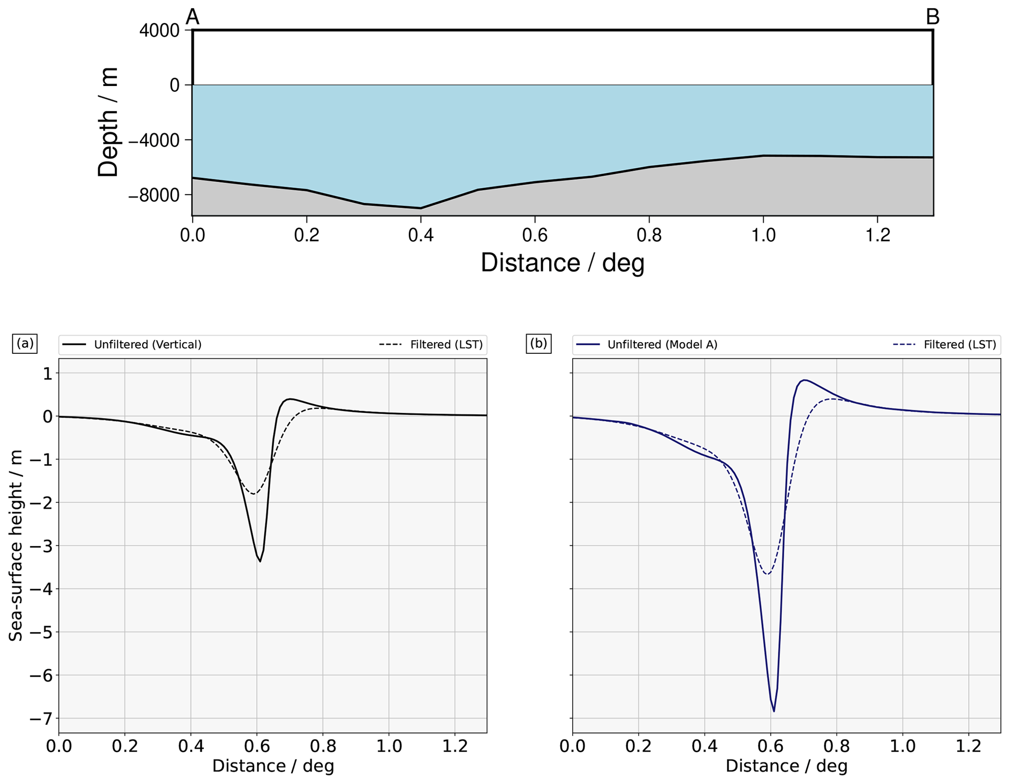
Figure 10 The picture refers to the 2007 event in the case of a source oriented to the northwest. The transect AB considered here is the one depicted in Fig. 9a. The upper panel illustrates the bathymetric profile along it. (a) The profiles are taken from the initial conditions in Fig. 9a, c, and e, considering only the vertical component. (b) The profiles are taken from the initial conditions in Fig. 9b, d, and f, considering the effect of the horizontal component through Model A.

Findings for the southeast dipping fault plane are presented in Figs. 11 and 12.

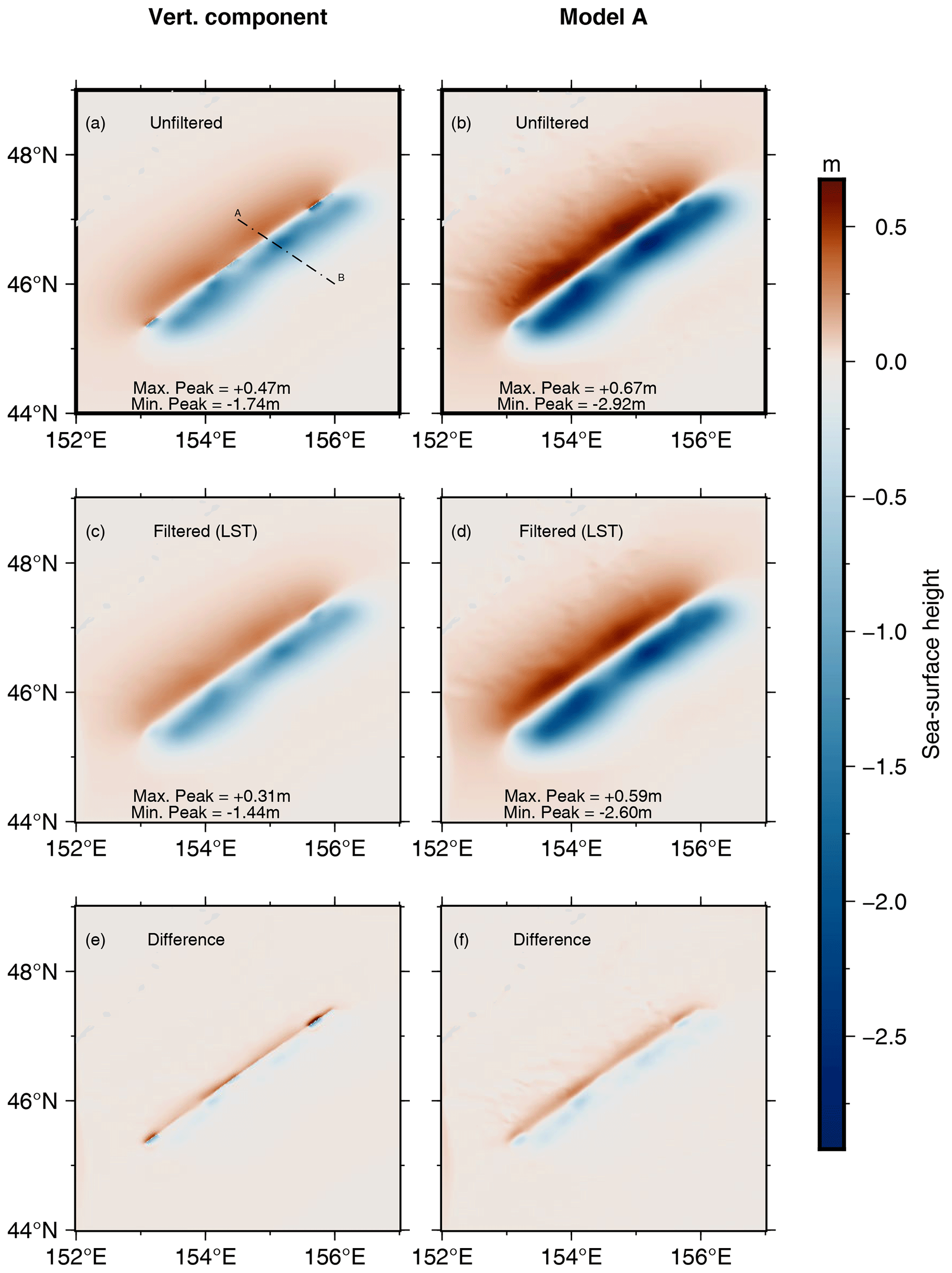
Figure 11 Results for the tsunamigenic earthquake that occurred on 13 January 2007. The fault plane is southeast dipping. Panel (a) depicts the transect AB where 1D profiles for all models have been considered. Panels (a), (c), and (e) present a sea surface perturbed by a vertical bottom deformation. Panels (b), (d), and (f) consider the contribution of the horizontal bottom displacement according to Model A. Panels (e) and (f) show the spatial distributions of the simple differences between the unfiltered and filtered initial conditions.

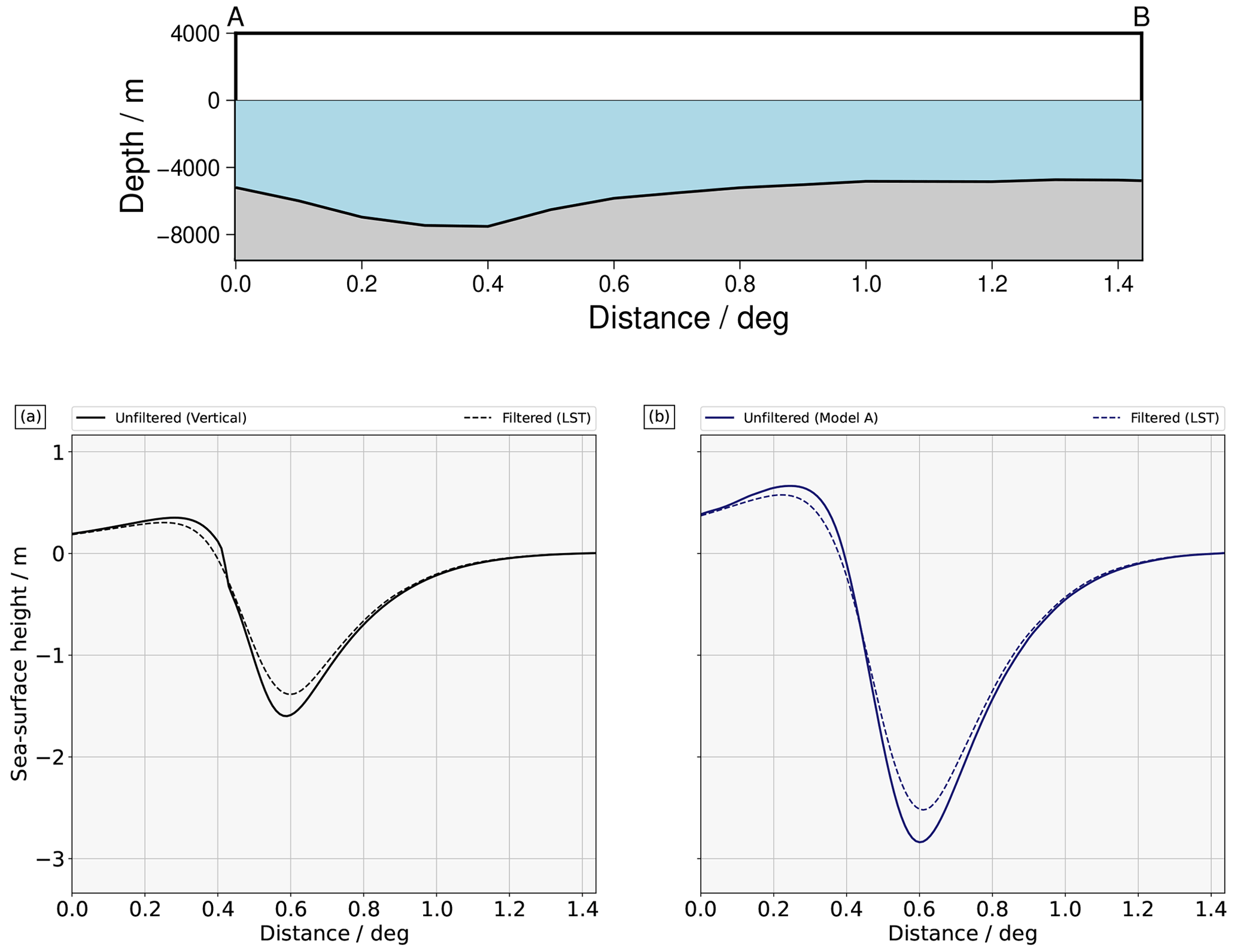
Figure 12 The picture refers the 2007 event in the case of a source oriented to the southeast. The transect considered here is the one depicted in Fig. 11a. Similarly to Fig. 10, the upper panel illustrates the bathymetric profile along it. (a) The profiles are taken from the initial conditions in Fig. 9a, c, and e, considering only the vertical component. (b) The profiles are taken from the initial conditions in Fig. 9b, d, and f, considering the effect of the horizontal component through Model A.

When replicating the ocean bottom deformation caused by the vertical component at sea level (Fig. 6), the negative peak reaches −1.74 m. Through our approach (LST), this value is heightened to −1.44 m. The positive crest is reduced from +0.47 to +0.31 m (Fig. 11a and c). When the horizontal component is taken into account using Model A, the top height is lessened by 0.08 m and the maximum depression by 0.32 m (Fig. 11d). Thus, for the southeast dipping scenarios, the effect of the filter is quite pronounced only on the stronger and shorter-wavelength trough. The smoothing effect is more significant for the vertical component, particularly affecting the two lobes of deformation positioned in the deep areas of the trench, as can be seen in Figs. 11f and 6c.

5.2 Discussion

In Sect. 5.1, we investigated events belonging to two major categories of earthquakes, both occurring in the central Kuril Islands: a megathrust, the 2006 event, and an outer-rise event, represented by the 2007 event. The low-pass filtering effect of the water column appears to be less pronounced for the megathrust as a result of the flatter dip of the subduction zone with respect to that of the crustal faults considered, which results in longer wavelengths. However, such a filtering effect is not negligible, as can be observed when looking at the mean relative percentage difference (MRPD) between the LST outputs and the unfiltered free-surface deformation for all seven models. To evaluate the MRPD, the unfiltered free-surface deformation ${\mathit{\xi }}_{\mathrm{0}}^{\mathrm{unf}}$ is obtained by copying the coseismic deformation at the free surface while subtracting the offset due to positive topographic elevation. In this way, only the perturbation of the water column is considered. The MRPD is then simply computed as

$$\begin{array}{}\text{(19)}& \widehat{e_{\mathrm{MRPD}}}=\mathrm{100}\times \mathrm{mean}\left(\mathrm{|}{\displaystyle \frac{{\mathit{\xi }}_{\mathrm{0}}^{\mathrm{LST}}-{\mathit{\xi }}_{\mathrm{0}}^{\mathrm{unf}}}{{\mathit{\xi }}_{\mathrm{0}}^{\mathrm{unf}}}}\mathrm{|}\right),\end{array}$$

where ${\mathit{\xi }}_{\mathrm{0}}^{\mathrm{LST}}$ is the initial free surface obtained through LST. For the 2006 megathrust in the central Kuril Islands, MRPD is 16.71 % for the vertical component, 21.80 % for Model A, and 17.01 % for Model B. The maximum differences between the unfiltered and filtered sea surface height distributions are roughly 3 times greater in uplift than in subsidence for this earthquake (third row in Fig. 7).

In contrast, the tsunami initial heights are substantially smoothed in the case of the 2007 outer-rise event. For the north dipping scenarios, the MRPD measured 33.03 % when a vertical-only coseismic deformation is considered and 46.05 % when Model A is taken into account. For the southeast dipping cases, such values are reduced to 16.24 % and 30.92 %, respectively. When considering the maximum spatial differences between the unfiltered and filtered initial conditions, they tend to be roughly 3 times greater in subsidence than in uplift for all the northwest dipping models. For the southeast cases, such differences are generally greater in subsidence than in uplift but doubled only in Model A. The areas of coseismic deformations following the megathrust event are in shallower waters if compared to those of interest for the outer rise. The average water depth is ∼2–3 km for the 2006 event, while it amounts to ∼7 km when looking at the 2007 event. Deeper sea depth implies more significant smoothing of the free-surface perturbation. Furthermore, the seafloor deformations associated with the megathrust have much greater length scales than those of the outer rise (as can be seen qualitatively in Fig. 6). The same reasoning can be applied to the 2007 event. Despite the similar source area, the two fault planes considered here are different in terms of both the direction and value of the dip angle. According to Lay et al. (2009), the southeast dipping plane exhibits a dip of 59°, while the northwest dipping plane has a dip of 47°, resulting in different extents of the coseismic deformation. When considering the southeast dipping fault plane, longer wavelengths can be qualitatively observed compared to the opposite dipping model (see Fig. 6b and c). Smaller wavenumbers should be smoothed in this case due to a broader seafloor deformation, contrasting with the opposite dipping fault plane where more than half of the deformation is attenuated. We note that for large wavelengths and relatively shallow depths (less than 1 km), there might be no need to account for a smoothing effect on the initial conditions (see Fig. 5).

For all the examined events, the horizontal movement of the sloping bottom significantly contributes to the perturbation of the free surface from the equilibrium position. However, we also demonstrate, for example in the case of the 2006 shock, that the initial condition is sensitive to how this horizontal contribution is modelled. In particular, Model A leads to an initial condition where both the maximum uplift and subsidence are more than twice the original unfiltered sea surface deformation. Considering the inelastic component of the coseismic deformation (Model B) would lead to a different outcome that depends on the size of the accretionary wedge. In general, the LST shows a systematic tendency to smooth the free-surface perturbation originated by Model A more, in all the scenarios considered. Furthermore, the filtering is more pronounced on the uplift or subsidence, depending on the mechanism of the triggering seismic event.

The LST algorithm is designed for practical applications. Its primary advantage is that it allows construction of a local database where, depending on the true sea depth, the scaled and smoothed tsunami unit initial conditions are stored to be used later. These unit solutions can be linearly combined, by weighting based on the corresponding coseismic deformation following an event. An example is the database for the central Kuril Islands, consisting of 89 700 cells. Such a database has been created in 59 min using 6 CPU nodes (dual-20-core Intel^® Xeon^® Gold 6248 clocked at 2.50 GHz). The execution time required to solve each cell varies with the local sea depth, but it ranges from ∼1 s to ∼1 min, provided that no inner parallelization is allowed. The linear recombination has been solved in ∼9 min using a single core Intel^® Core™ i7-10510U CPU clocked at 1.80 GHz. The spatial resolution used is 1 arcmin, and we noted that an increase/decrease in the execution time by a factor of ∼4 is obtained by doubling/halving the grid resolution. The term local database means that the solution depends on the coordinates and local bathymetry of the region. There are plans to distribute it as a service in the future, offering a set of unit solutions based on the corner coordinates of the region of interest. To further enhance efficiency, some proposed ideas include the following.

1. Since the model's dependence on resolution and water depth is discussed in Sect. 4, a general database could be constructed considering typical cell dimensions and incremental bathymetric values. This database could then be matched to geographic coordinates by applying latitude correction and binning sea depth values.

2. The tool could be redesigned to eliminate the need for database construction, potentially parallelizing it to leverage GPU architecture.

6 Conclusions

To enhance the computational efficiency and the applicability of the Laplacian smoothing algorithm proposed by Nosov and Kolesov (2011), we adopt a strategy informed by numerical analysis. This involves constructing a database of unit initial conditions tailored for tsunami simulations. These sources undergo high-frequency content filtering. Initially addressing the problem in one dimension, we explore the convergence of the integral describing the water height distribution at the sea surface. Our findings reveal that wavenumbers less than $\frac{\mathrm{5}}{H}$, with H denoting the flat bathymetry within the cell, are necessary to avoid artefacts when modelling tsunami generation in classic linear potential theory. We conduct a comprehensive comparison of various numerical quadratures against reference analytic–numeric solutions, evaluating efficiency and accuracy. The model is an analytical solution to the 3D Laplace equation for the fluid velocity potential, which is linear if the sea bottom does not undergo significant variations within a radius of few wavelengths. Leveraging this linearity and the fact that sea bottom deformation is linear with respect to the slip, we construct a database of elementary initial conditions. Each entry is scaled by the corresponding bottom displacement. Thus, the methodology allows for the consideration of an arbitrary bottom topography. This database is then applied to nine different models to obtain the sea surface height distribution following the megathrust and outer-rise events near the central Kuril Islands in late 2006 and early 2007. We consider the contribution of the vertical component and the impact of horizontal movement of the bottom, highlighting the significance of the latter in earthquakes near steep slopes. Additionally, we demonstrate the sensitivity of the chosen model in representing horizontal components, contingent on the affected area. We observe that the smoothing effect of the water column is particularly evident when considering the horizontal component, and it is relatively less pronounced in cases of shallow megathrust events, where wavelengths significantly exceed the water depth compared to crustal earthquakes. Despite this, even for interplate earthquakes, the smoothing effect cannot be considered negligible, as it results in an approximately 20 % decrease in the sea height spatial distribution. We also observe that in general such a smoothing effect is more pronounced on the uplifted or subsided free surface, depending on the mechanism of the seismic event and on its position relative to the coast. In the future, a possible development could involve considering the case of a time-dependent rupture and assessing its impact on the free-surface deformation. The proposed approach, as well as its applicability to any seafloor displacement and variable bottom topography, may be relevant for practical applications. A further enhancement of its computation performance through HPC architecture could allow the methodology to be used for those studies that require a huge number of simulations, such as long-term probabilistic tsunami hazard assessment (PTHA), and for real-time applications where the tsunami forecasting needs to be addressed quickly and with the highest-possible accuracy. A further step will be that of studying the sensitivity of the model with respect to different wavelengths and to assess the consequent impact on the inundation.

Appendix A: Acronyms

LED	Local extended domain
GAQ	Global adaptive quadrature
GLQ	(Adapted) Gauss–Legendre quadrature
FQ	(Adapted) Filon quadrature
RMSE	Root-mean-square error
LST	Laplacian smoothing tool
MRPD	Mean relative percentage error