An improved dynamic bidirectional coupled hydrologic–hydrodynamic model for efficient flood inundation prediction

To improve computational efficiency while maintaining numerical accuracy, coupled hydrologic–hydrodynamic models based on non-uniform grids are used for flood inundation prediction. In these models, a hydrodynamic model using a fine grid can be applied to flood-prone areas, and a hydrologic model using a coarse grid can be used for the remaining areas. However, it is challenging to deal with the separation and interface between the two types of areas because the boundaries of the flood-prone areas are time dependent. We present an improved Multigrid Dynamical Bidirectional Coupled hydrologic–hydrodynamic Model (IM-DBCM) with two major improvements: (1) automated non-uniform mesh generation based on the D-infinity algorithm was implemented to identify the flood-prone areas where high-resolution inundation conditions are needed and (2) ghost cells and bilinear interpolation were implemented to improve numerical accuracy in interpolating variables between the coarse and fine grids. A hydrologic model, the 2D nonlinear reservoir model, was bidirectionally coupled with a 2D hydrodynamic model that solves the shallow-water equations. Three cases were considered to demonstrate the effectiveness of the improvements. In all cases, the mesh generation algorithm was shown to efficiently and successfully generate high-resolution grids in those flood-prone areas. Compared to the original M-DBCM (OM-DBCM), the new model had lower root-mean square errors (RMSEs) and higher Nash–Sutcliffe efficiencies (NSEs), indicating that the proposed mesh generation and interpolation were reliable and stable. It can be adequately adapted to the real-life flood evolution process in watersheds and provide practical and reliable solutions for rapid flood prediction.

1 Introduction

Floods are the most frequent natural disasters that seriously harm human health and economic growth. Numerical models are critical for predicting flooding processes to help prevent or mitigate the damaging effects of floods on people and communities (Bates, 2022). Coupled hydrologic–hydrodynamic models are widely used to translate the amount of rainfall obtained from weather forecasting models or rain gauge observations into surface inundation (Xia et al., 2019).

Coupled hydrologic–hydrodynamic models can be generally divided into external (one-way) and internal (two-way) coupling models (see Fig. 1). The external coupling models utilize hydrographs obtained from hydrologic models as inputs for hydrodynamic models in a fixed position, providing a one-way transition (Schumann et al., 2013; Feistl et al., 2014; Choi and Mantilla, 2015; Bhola et al., 2018; Wing et al., 2019). It is a powerful tool for watershed flood simulation, in particular for large spatial and temporal scales, due to its convenience in model construction. However, this one-way flow information cannot capture the mutual interaction between runoff production and flood inundation, and the fixed interface is inconsistent with the actual flood process, where the inflow discharge positions, flow path and discharge values change with accumulating rainfall.

Figure 1 Classifications of coupled hydrologic and hydrodynamic models.

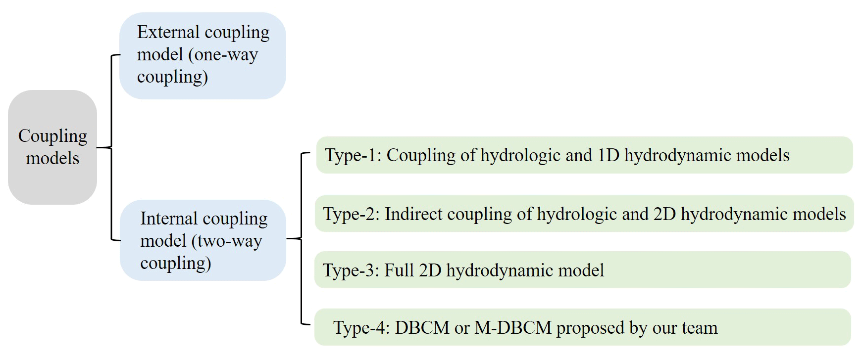
The two-way coupling models are further divided into the coupled hydrologic–1D hydrodynamic model (HH1D), indirect coupled hydrologic-2D–hydrodynamic models (ICM2D), full 2D hydrodynamic models (HM2D) and dynamic bidirectional coupling models (DBCM or M-DBCM) proposed by author's team. In the HH1D, the discharge obtained from the hydrologic model is treated as a mass source of the 1D hydrodynamic model, while the water depth calculated in the 1D hydrodynamic model is fed back into a hydrologic model such as the coupled Mike SHE and Mike 11 model (Thompson et al., 2004). The application of 1D modelling of overland flow is limited when developing precise and reliable flood maps in 2D inundation regions.

In order to overcome the lack of 2D hydrodynamic simulation in HH1D, the ICM2D is proposed, where the runoff first flows into 1D rivers and then discharges into the 2D inundation regions (Seyoum et al., 2012; Chen et al., 2017, 2018). For example, Mike SHE and Mike 11 are coupled to form Mike Urban, and Mike 11 and Mike 21 are dynamically coupled to form Mike Flood. The indirect coupling between the hydrologic and the 2D hydrodynamic models can be developed by coupling Mike Urban and Mike Flood. The 1D hydrodynamic model is a connection channel between the hydrology and the 2D hydrodynamic models. Compared to the HH1D, this coupling type has satisfactory and acceptable accuracy and is widely used. As the 2D hydrodynamic model is only calculated in local inundation regions, its computational efficiency is greatly improved in comparison to the HM2D. However, the ICM2D assumes that the water first discharges into the 1D rivers and then flows from 1D rivers to the 2D regions. The hydrologic model is not directly coupled with the 2D hydrodynamic model, which is inconsistent with the actual flood processes. In reality, water may be discharged into both 1D channels and 2D waterbodies simultaneously, and the hydrologic and 2D hydrodynamic models should be linked directly. Direct coupling of hydrologic and 2D hydrodynamic models can physically reflect the flood processes, a fact which deserves more attention.

In HM2D, the 2D hydrodynamic model is used to simulate the overland flow (runoff routing and flood inundation), and the runoff generation serves as its mass source term (Singh et al., 2011; Garcia-Navarro et al., 2019; Hou et al., 2020; Costabile and Costanzo, 2021). It has satisfactory and acceptable numerical accuracy and has been widely used. But the development and simulation of HM2D require high-resolution topographic data at the catchment scale and extensive computational time, which hinder its application in large-scale flood forecasting (Kim et al., 2012). In HEC-RAS (US Army Corps of Engineers, 2023), for instance, the flooding process in 1D rivers was simulated by a 1D hydrodynamic model, whereas the flooding process in 2D regions was simulated using 2D diffusion wave equations (DWEs) or shallow-water equations (SWEs). If the 2D regions are discretized into finer grids and the 2D SWEs is applied, the 1D hydrodynamic model is coupled with the 2D SWEs. It has high numerical accuracy but is computationally prohibitive for large-scale applications. Conversely, if the 2D regions are discretized into coarse grids and the 2D DWEs is applied, the 1D hydrodynamic model is coupled with the 2D DWEs, which can expand the application scale at the cost of reducing the accuracy.

Jiang et al. (2021) proposed a DBCM based on uniform structured grids, where the hydrologic and 2D hydrodynamic models were coupled in a two-way manner and the coupling interface of these two models was time dependent. The model can automatically evolve the surface flow and fully consider the flow states with both mass and momentum transfer. However, because uniform grids were adopted in DBCM, it inevitably increased the computational cost and time, especially in large watersheds.

An essential consideration to reduce computational time is mesh coarsening (Caviedes-Voullième et al., 2012). Adaptive mesh refinement (AMR) has been used to optimize the grid resolution during flood simulations (Donat et al., 2014; Hu et al., 2018; Ghazizadeh et al., 2020; Ding et al., 2021; Kesserwani and Sharifian, 2023). Aiming to increase computational efficiency by reducing computing nodes, it adjusts grid size for local grid refinement by domain features or flow conditions. Yu (2019) used quad-tree grids to divide the computational domain and applied the DBCM to simulate the flooding process. DBCM needs to segment and merge the grid elements repeatedly during the calculation, which can be time-consuming and can offset the calculation time saved by the optimized grid. AMR is commonly employed in scenarios where flow characteristics exhibit abrupt variations such as aerodynamic shock waves, hydraulic jumps and seismic tsunami waves. Capturing discontinuous solutions necessitates local grid refinement, with the location of the refinement dynamically adapting to the position of the discontinuities. AMR is indispensable for this purpose. Flow characteristic variations arising from abrupt geometric changes in the computational domain can be captured using static local refinement grids, provided that the extent of these changes is limited. This approach offers computational time savings.

Static non-uniform grids simplify the grid generation procedure compared to AMR (Caviedes-Voullième et al., 2012; Hou et al., 2018; Bomers et al., 2019; Ozgen-Xian et al., 2020). Compared to uniform grids and AMR, it can not only reduce computational nodes but also use different time steps in different grid sizes to further reduce computation time. Shen et al. (2021) and Shen and Jiang (2023) divided the computational domain based on static multi-grids, where different grid size ratios of coarse to fine grids were designed. However, there were two limitations to this scheme. One limitation is that the grids need to be generated manually, which can be subjective and uncertain. It also needs a heavy workload, especially for large watersheds. Besides the grid generation, the variable interpolation between the coarse and fine cells was also not reasonable. There are shared and hanging nodes at the interpolation interface. Shen et al. (2021) assumed the variables at the shared nodes were equal to those at the cell centre, and the hanging nodes were calculated according to the shared nodes. The results showed that this scheme has unsatisfactory accuracy and frequently fails to converge. Although the multi-grid-based model can reduce computational time, there are remarkable challenges such as the grid partition technique, determination of coarse and fine regions, and variable interpolation between coarse and fine grids.

The objective of this study is to develop an integrated system that fully couples the hydrologic and 2D hydrodynamic models, to utilize an automated method for efficient multi-grid mesh generation, and to resolve variable interpolation between coarse and fine grids more accurately. An improved dynamic bidirectional coupling model (IM-DBCM) is presented, where the 2D nonlinear reservoir (NLR) model was coupled with the 2D hydrodynamic model through a coupling moving interface (CMI). The D-infinity algorithm was implemented to divide the computational domain into non-uniform grids automatically. Ghost cells (i.e. virtual cells located on the boundaries of the computational domain) and bilinear interpolation were used to interpolate variables between the coarse and fine grids. Three case studies were conducted, and the simulation results were compared with the original M-DBCM (OM-DBCM) to evaluate the effectiveness of the improvements.

2 Methodology

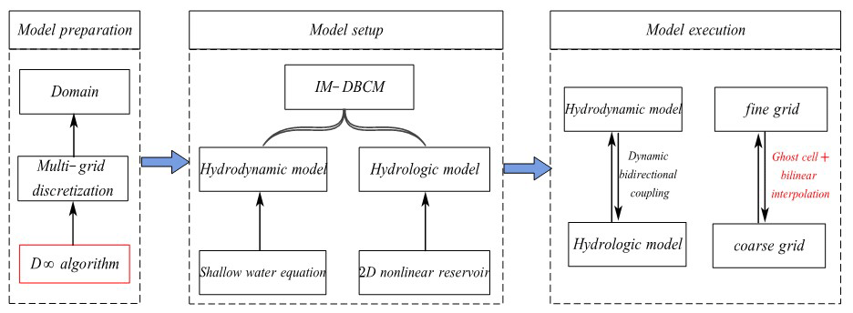
The Fortran programming language was adopted to apply to the coupling model. The framework of IM-DBCM is illustrated in Fig. 2. The model consists of two components: a hydrologic model (i.e. 2D NLR) that simulates the runoff generation and routing and a 2D hydrodynamic model simulating the flood inundation process. Before the model was set up, it was first necessary to design the grids. Static multi-grids were applied to the model. For the model execution, the variable interpolation between coarse and fine grids and the coupling of hydrologic and hydrodynamic models are the two main issues that must be addressed.

Figure 2 Framework of the IM-DBCM.

2.1 Automated multi-grid generation

The design of computational grids that are scalable and suitable for all applications associated with flood models is challenging. Grid generation can be considered a model preprocess, which is the foundation of flood simulation and can influence both computational accuracy and efficiency. In this study, a multi-grid generation method is proposed, based on the D-infinity algorithm, to generate refined grid cells in flood-prone areas where high-resolution representation of topographic features is essential for flood simulation, while discretizing the rest of the domain using coarse grids. The D-infinity algorithm is a method of representing flow directions based on triangular facets in the grid digital elevation model (DEM) proposed by Tarboton (1997). It allocates the flow fractionally to each lower neighbouring grid in proportion to the slope toward that grid. The flow direction is determined as the direction of the steepest downward slope on the eight triangular facets formed across a 3×3 pixel window centred on the pixel of interest, which was detailed by Tarboton (1997). Compared to the D8 algorithm, where the flow is discretized into only one of eight possible directions separated by 45°, the D-infinity algorithm is more reasonable and accurate for delineating the actual river trend.

Figure 3 Grid generation based on the D-infinity algorithm.

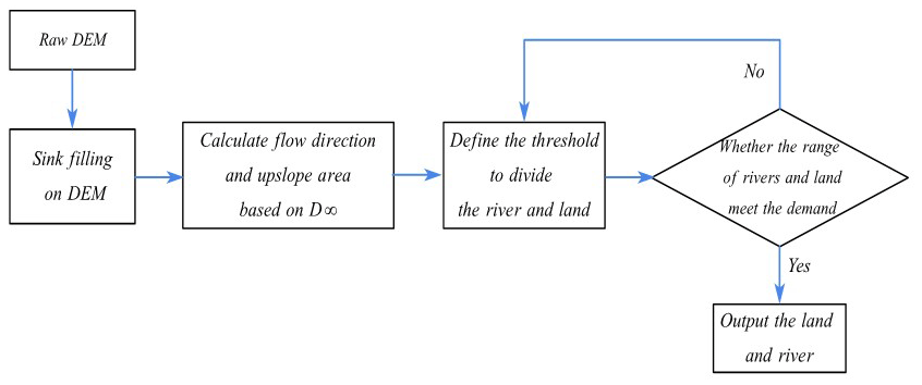
The process of discretizing computational domain based on the D-infinity algorithm is shown in Fig. 3. First, a raw DEM was prepared and sink filling was performed on the DEM. Second, the D-infinity algorithm was applied to determine the flow direction on the grids. Subsequently, the upslope area, defined as the total catchment area that is upstream of a grid centre or short length of contour (Moore et al., 1991), was calculated based on the flow direction. Finally, an area threshold was defined to identify the slope lands and derive the river drainage networks from the accumulated drainage areas. In a grid cell, if the upslope area was larger than the predefined threshold, it was considered a river drainage network; otherwise, it was defined as slope lands. The generated slope lands and river network were verified through field surveys or satellite-image-based estimates. Generally, the river drainage networks present low slopes and hydraulic conveyance, which are subject to flooding. Areas prone to waterlogging, characterized by persistent water saturation, frequently occur adjacent to rivers. The dynamics of inundation in these low-lying zones constitute a central aspect of our investigation. Therefore, these areas should be discretized using fine grids to represent the flooding process in high resolution. However, in the slope lands, fine grids were not required and coarse grids were used to improve computational efficiency. Because the regions of interest were of high resolution, the reliability of the prediction did not deteriorate even though the number of grid cells was considerably reduced, which can increase model efficiency and capability for flood simulations over large domains. Compared to manual work, grid generation based on the D-infinity algorithm can reduce both workload and time.

AMR dynamically adapts the grid resolution during the simulation, refining the grid locally based on domain characteristics or flow conditions. AMR is commonly employed in scenarios where flow characteristics exhibit abrupt variations such as aerodynamic shock waves, hydraulic jumps and tsunami waves. Capturing discontinuous solutions necessitates local grid refinement, with the location of refinement dynamically adapting to the position of the discontinuities. Consequently, AMR is indispensable. However, AMR needs to segment and merge the grid elements repeatedly during the calculation, which can be time-consuming and offset the calculation time saved by the optimized grid. Besides, the mesh generation and flood simulation were compiled in the same code base, which increased the computation cost and time.

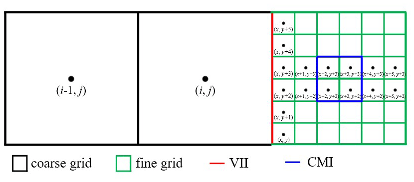
Figure 4 Schematic diagram of grid generation where i and j are the coordinates of the coarse grid, x and y are the coordinates of the fine grid, VII is the variable interpolation interface, and CMI is the coupling moving interface.

Flow characteristic variations arising from abrupt geometric changes in the computational domain can be captured using static local refinement grids, provided that the extent of these changes is limited. This approach offers computational time savings. In flood simulations, inundation regions are typically situated in low-lying 2D regions. The outer boundary of the inundation regions can be determined using DEM or calculated by hydrologic models. The D-infinity algorithm was employed to pre-emptively estimate the extent of these areas, providing enhanced computational efficiency relative to AMR and obviating the uncertainty and complexity associated with manual subdivision of the computational domain.

A schematic of grid generation is shown in Fig. 4. Two types of connecting interfaces are presented, which divide the computing domain into three parts. The first type is the red line (variable interpolation interface; VII) between the coarse and fine grids. The grid cell size changes suddenly on both sides of this line. The second type (coupling moving interface; CMI) is marked in blue on fine grids, which is movement- and time-dependent. The first part represents the coarse-grid areas, where the hydrologic model is used to simulate rainfall–runoff. The other two parts are located in the fine-grid areas. The regions between VII and CMI are defined as intermediate-transition zones, where the hydrologic model is used to simulate the flooding process. These transition zones facilitate the application of different time steps in different grid cell sizes to improve computational efficiency. The hydrologic and hydrodynamic models are dynamically coupled to represent the flooding process on fine grids, and the CMI is a coupling boundary.

2.2 Variable interpolation between coarse and fine grids

During flow computation, if a cell has a neighbour of a different size, interpolation may be required to approximate variables in certain locations so that the governing equation can be solved smoothly. An example is presented in Fig. 5a, where the coarse grid has two eastern neighbours that are half its size. In this case, the variable values of the smaller cells are obtained from those of the larger cells. In the traditional method, these variables are directly calculated using certain interpolation methods. There are shared (P₁, P₂) and hanging (Q) nodes at the interface between the coarse and fine grids. In Shen et al. (2021), the variable values on shared nodes can be transmitted directly, while the values on hanging nodes are obtained by linear interpolation of the shared nodes. This method is simple, feasible and easy to use. However, the variable values are stored at the cell centre, and there are no values at the interface nodes. Shen et al. (2021) assumed that the values at the interface nodes were equal to that at the cell centre. It is inaccurate to make such an assumption, as it can cause errors, and the resulting error will increase as the cell size increases.

Figure 5 Variable interpolation between coarse and fine grids: (a) from coarse to fine grids and (b) from fine to coarse grids.

To overcome these drawbacks, ghost cells and the bilinear interpolation method were used to interpolate variables between coarse and fine grids. Figure 5a shows the variable interpolation between the coarse and fine grids. Two ghost fine cells were created, which were overlaid with partial coarse grids. The variables at the ghost fine cells were interpolated through the coarse and fine grids between the interface, which were then used as the boundary conditions for the calculation of the fine grids at the next time step. The bilinear interpolation method was applied. Variable interpolation may involve variables at locations c₁,c₂, c₃, $f_{v\mathrm{1}}^{\prime }$, $f_{v\mathrm{2}}^{\prime }$, f₁ and f₂. As the variables are stored at the cell centre, the variables at c₁, c₂, c₃, f₁ and f₂ are available directly. The values at $f_{v\mathrm{1}}^{\prime }$ and $f_{v\mathrm{2}}^{\prime }$ are obtained via natural neighbour interpolation as follows:

$$\begin{array}{}\text{(1)}& {\displaystyle }& {\displaystyle }{U}_{f_{v\mathrm{1}}^{\prime }}=U_{c_{\mathrm{1}}}+{\displaystyle \frac{U_{c_{\mathrm{2}}}-U_{c_{\mathrm{1}}}}{y_{c_{\mathrm{2}}}-y_{c_{\mathrm{1}}}}}\left(y_{f_{v\mathrm{1}}^{\prime }}-y_{c_{\mathrm{1}}}\right),\text{(2)}& {\displaystyle }& {\displaystyle }{U}_{f_{v\mathrm{2}}^{\prime }}=U_{c_{\mathrm{3}}}+{\displaystyle \frac{U_{c_{\mathrm{1}}}-U_{c_{\mathrm{3}}}}{y_{c_{\mathrm{1}}}-y_{c_{\mathrm{3}}}}}\left(y_{f_{v\mathrm{2}}^{\prime }}-y_{c_{\mathrm{3}}}\right),\end{array}$$

where $U_{f_{v\mathrm{1}}^{\prime }}$, $U_{f_{v\mathrm{2}}^{\prime }}$, $U_{c_{\mathrm{1}}}$, $U_{c_{\mathrm{2}}}$ and $U_{c_{\mathrm{3}}}$ are the variables at locations $f_{v\mathrm{1}}^{\prime }$, $f_{v\mathrm{2}}^{\prime }$, c₁, c₂ and c₃, respectively, and $y_{f_{v\mathrm{1}}^{\prime }}$, $y_{f_{v\mathrm{2}}^{\prime }}$, $y_{c_{\mathrm{1}}}$, $y_{c_{\mathrm{2}}}$ and $y_{c_{\mathrm{3}}}$ are the coordinates in y directions at $f_{v\mathrm{1}}^{\prime }$, $f_{v\mathrm{2}}^{\prime }$, c₁, c₂ and c₃, respectively.

Then, the variables of ghost fine cells at f_v1 and f_v2 can be calculated based on those at $f_{v\mathrm{1}}^{\prime }$ and $f_{v\mathrm{2}}^{\prime }$ as follows:

$$\begin{array}{}\text{(3)}& {\displaystyle }& {\displaystyle }{U}_{f_{v\mathrm{1}}}=U_{f_{v\mathrm{1}}^{\prime }}+{\displaystyle \frac{U_{f_{\mathrm{1}}}-U_{f_{v\mathrm{1}}^{\prime }}}{x_{f_{\mathrm{1}}}-x_{f_{v\mathrm{1}}^{\prime }}}}\left(x_{f_{v\mathrm{1}}}-x_{f_{v\mathrm{1}}^{\prime }}\right),\text{(4)}& {\displaystyle }& {\displaystyle }{U}_{f_{v\mathrm{2}}}=U_{f_{v\mathrm{2}}^{\prime }}+{\displaystyle \frac{U_{f_{\mathrm{2}}}-U_{f_{v\mathrm{2}}^{\prime }}}{x_{f_{\mathrm{2}}}-x_{f_{v\mathrm{2}}^{\prime }}}}\left(x_{f_{v\mathrm{2}}}-x_{f_{v\mathrm{2}}^{\prime }}\right),\end{array}$$

where $U_{f_{v\mathrm{1}}}$ and $U_{f_{v\mathrm{2}}}$ are the variables of the ghost fine cells; $U_{f_{\mathrm{1}}}$ and $U_{f_{\mathrm{2}}}$ are the variables at f₁ and f₂, respectively, which were calculated in the last time step; and $x_{f_{\mathrm{1}}}$, $x_{f_{\mathrm{2}}}$, $x_{f_{v\mathrm{1}}}$, $x_{f_{v\mathrm{2}}}$, $x_{f_{v\mathrm{1}}^{\prime }}$ and $x_{f_{v\mathrm{2}}^{\prime }}$ are the coordinates in x directions at f₁, f₂, f_v1, f_v2, $f_{v\mathrm{1}}^{\prime }$ and $f_{v\mathrm{2}}^{\prime }$, respectively.

The values at f_v1 and f_v2 were used as the boundary conditions for the calculation of fine grids.

The variable interpolation from fine to coarse grids is presented in Fig. 5b, where one ghost coarse cell was established. The variables of ghost coarse cells were determined according to the fine and coarse grids between the interface. The variable interpolation may involve variables at locations $c_v^{\prime }$, c₁, f₁ or f₂. As the variables are stored at the cell centre, the variables at c₁, f₁ and f₂ are available directly. The values at $c_v^{\prime }$ are obtained via natural-neighbour interpolation as follows:

$$\begin{array}{}\text{(5)}& U_{c_v^{\prime }}=U_{f_{\mathrm{2}}}+{\displaystyle \frac{U_{f_{\mathrm{1}}}-U_{f_{\mathrm{2}}}}{y_{f_{\mathrm{1}}}-y_{f_{\mathrm{2}}}}}\left(y_{c_v^{\prime }}-y_{f_{\mathrm{2}}}\right),\end{array}$$

where $U_{c_v^{\prime }}$, $U_{f_{\mathrm{1}}}$ and $U_{f_{\mathrm{2}}}$ are the variables at $c_v^{\prime }$, f₁ and f₂, respectively, and $y_{c_v^{\prime }}$, $y_{f_{\mathrm{1}}}$ and $y_{f_{\mathrm{2}}}$ are the coordinates in y direction at $c_v^{\prime }$, f₁ and f₂, respectively.

And then, the variables of ghost coarse cells at c_v can be calculated based on those at $c_v^{\prime }$ and c₁ as follows:

$$\begin{array}{}\text{(6)}& U_{c_v}=U_{c_v^{\prime }}+{\displaystyle \frac{U_{c_{\mathrm{1}}}-U_{c_v^{\prime }}}{x_{c_{\mathrm{1}}}-x_{c_v^{\prime }}}}\left(x_{c_v}-x_{c_v}^{\prime }\right),\end{array}$$

where $U_{c_v}$ is the variable of a ghost fine cell; $U_{c_{\mathrm{1}}}$ is the variable at c₁, which was calculated in the last time step; and $x_{c_{\mathrm{1}}}$, $x_{c_v}^{\prime }$ and $x_{c_v}$ are the coordinates in x direction at c₁, $c_v^{\prime }$ and c_v, respectively.

The values at c_v were used as boundary conditions for the calculation of coarse grids at the next time step.

On both sides of the interface between coarse and fine grids, the hydrologic model was used to simulate the flood process. In the hydrologic model applied to the IM-DBCM, the Manning equation is employed to simulate surface runoff processes. As a linear partial differential equation, the Manning equation lacks a nonlinear convection term. Consequently, the flow state undergoes relatively smooth changes without exhibiting discontinuous solutions. Linear interpolation is applied to interpolate variables between coarse and fine grids, with the interpolated values falling within the range defined by the maximum and minimum values of the interval. This interpolation ensures that the result lies between these bounds, precluding the occurrence of increased flow at the interface of coarse- and fine-grid transitions.

2.3 Numerical models

2.3.1 Hydrologic model

In this study, a 2D NLR model referring to the runoff calculation in the Storm Water Management Model (SWMM) including water balance and Manning equations was used to simulate rainfall–runoff. In SWMM, the watershed is divided into many water tanks or reservoirs, where a 1D NLR model including water balance and 1D Manning equations is used to simulate the runoff (Rossman, 2015). It is a simple and efficient method to calculate the runoff routing. In reality, however, the runoff routing is a 2D process, so it is not accurate to calculate the 2D runoff routing using a 1D NLR model. Also, it is difficult to directly couple the 1D NLR model with a 2D hydrodynamic model. Therefore, the 2D NLR model was used to simulate the 2D surface runoff routing in this study, as shown in Eqs. (7)–(11). The effects of subsurface runoff are assumed to be negligible, which is reasonable for the intense rainfall-induced flood events considered in this study (Hou et al., 2018; Li et al., 2021).

$$\begin{array}{}\text{(7)}& {\displaystyle }\begin{array}{rl}{\displaystyle \frac{V_i^{n+\mathrm{1}}-V_i^n}{\mathrm{\Delta }t}}& ={\left(Q_x\right)}_{\mathrm{in}i}-{\left(Q_x\right)}_{\mathrm{out}i}+{\left(Q_y\right)}_{\mathrm{in}i}\\ & -{\left(Q_y\right)}_{\mathrm{out}i}+A_i{q}_{\mathrm{r}i}^n,\end{array}\text{(8)}& {\displaystyle }{\left(Q_x\right)}_{\mathrm{in}i}-{\left(Q_x\right)}_{\mathrm{out}i}=-\sum _{l=\mathrm{1}}^L{\left(q_{x\mathrm{\Gamma }}^n\cdot n_x\right)}_l\mathrm{\Delta }{L}_l,\text{(9)}& {\displaystyle }{\left(Q_y\right)}_{\mathrm{in}i}-{\left(Q_y\right)}_{\mathrm{out}i}=-\sum _{l=\mathrm{1}}^L{\left(q_{y\mathrm{\Gamma }}^n\cdot n_y\right)}_l\mathrm{\Delta }{L}_l,\text{(10)}& {\displaystyle }{q}_x={\displaystyle \frac{h^{\mathrm{5}/\mathrm{3}}{S}_x^{\mathrm{1}/\mathrm{2}}}{n_{\mathrm{r}}}},\text{(11)}& {\displaystyle }{q}_y={\displaystyle \frac{h^{\mathrm{5}/\mathrm{3}}{S}_y^{\mathrm{1}/\mathrm{2}}}{n_{\mathrm{r}}}},\end{array}$$

where the superscripts n and n+1 are the time steps; V is the water volume of the grid (m³); (Q_x)_in i and (Q_x)_out i are the inflow and outflow of grid i in x direction (m³ s⁻¹); (Q_y)_in i and (Q_y)_out i are the inflow and outflow of grid i in y direction (m³ s⁻¹); q_r i indicates the runoff rate of grid i (mm h⁻¹), which is rainfall intensity minus infiltration rate; A_i is the area of grid i (m²); q_x and q_y are the unit discharge stored at the cell centre along x and y directions (m² s⁻¹), with h, u and v being water depth (m) and flow velocity (m s⁻¹) in x and y directions, respectively; q_xΓ and q_yΓ are the unit discharge at grid boundary in x and y directions, respectively (m² s⁻¹), which are calculated based on q_x and q_y; ΔL_l is the side length of the grid (m); l=1, 2, 3, …, L is the number of edges of the cell; n_r is the Manning roughness coefficient; S_x and S_y are water level gradients along x and y directions, respectively; and $S_x=-\partial (z_b+h)/\partial x$ and $S_y=-\partial (z_b+h)/\partial y$, where z_b is the surface elevation.

2.3.2 Hydrodynamic model

The 2D SWEs, consisting of mass and momentum conservation equations (Toro, 2001), were used to represent the hydrodynamic model.

$$\begin{array}{}\text{(12)}& {\displaystyle \frac{\partial U}{\partial t}}+{\displaystyle \frac{\partial F}{\partial x}}+{\displaystyle \frac{\partial G}{\partial y}}=S,\end{array}$$

$$\begin{array}{ll}{\displaystyle }& {\displaystyle }U=\left(\begin{array}{l}h\\ hu\\ hv\end{array}\right),F=\left(\begin{array}{l}hu\\ huu+g{h}^{\mathrm{2}}/\mathrm{2}\\ huv\end{array}\right),\\ {\displaystyle }& {\displaystyle }G=\left(\begin{array}{l}hv\\ huv\\ hvv+g{h}^{\mathrm{2}}/\mathrm{2}\end{array}\right),\\ {\displaystyle }& {\displaystyle }S=\left(\begin{array}{l}{q}_r\\ -gh\frac{\partial z}{\partial x}-\frac{g}{C^{\mathrm{2}}}u\sqrt{u^{\mathrm{2}}+v^{\mathrm{2}}}\\ -gh\frac{\partial z}{\partial y}-\frac{g}{C^{\mathrm{2}}}v\sqrt{u^{\mathrm{2}}+v^{\mathrm{2}}}\end{array}\right),\end{array}$$

where U represents the conserved variables; F and G are the convection terms in x and y directions; S is the source term; and C is Chézy's coefficient, $C=\frac{\mathrm{1}}{n_{\mathrm{r}}}{R}^{\mathrm{1}/\mathrm{6}}$, where n_r is the Manning roughness coefficient and R is the hydraulic radius.

The finite volume method for conservative scheme was used to solve the SWEs, which can ensure local mass and momentum conservation in each control volume cell. Equation (12) can be discretized based on structured grids as follows:

$$\begin{array}{}\text{(13)}& \begin{array}{rl}{U}_{i,j}^{n+\mathrm{1}}& =U_{i,j}^n-{\displaystyle \frac{\mathrm{\Delta }t}{A_{i,j}}}\sum _{l=\mathrm{1}}^L\left[F^l\left(U_{i,j}^n\right)\mathrm{d}y-G^l\left(U_{i,j}^n\right)\mathrm{d}x\right]\\ & +{\displaystyle \frac{\mathrm{\Delta }t}{A_{i,j}}}S\left(U_{i,j}^n\right),\end{array}\end{array}$$

where the superscripts n and n+1 are the time steps, the subscripts i and j refer to the grid i and j, and dx and dy are the grid edge lengths. The meaning of the other symbols is the same as before.

The Harten–Lax–van Leer contact (HLLC) approximate Riemann solver was used to solve the convection term. The second-order accuracy in temporal and spatial discretization was obtained based on the Runge–Kutta method and Monotone Upstream-centred Schemes for Conservation Laws (MUSCL; Van Leer, 1979). The solution of SWEs has been detailed in many references (e.g. Toro, 2001).

2.4 Dynamic bidirectional coupling of hydrologic and hydrodynamic models

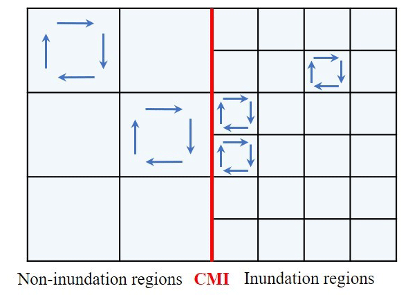
The hydrologic and hydrodynamic models were coupled dynamically and bidirectionally. A water depth threshold was defined in advance and used to determine the state of the cell. In a grid cell, if the water depth was lower than the predefined threshold, it was defined as a non-inundation region where the hydrologic model was applied. Conversely, if the water depth was higher than the threshold, it was considered an inundation region where the 2D hydrodynamic model was applied. When the rainfall intensity increased, the water depth increased because of the gradual accumulation of surface water volume. Once the water depth exceeded the predefined threshold, the non-inundation regions defined in the last time step were able to change to inundation regions. The inflow discharge positions, flow path and discharge values subsequently changed. Therefore, a CMI was formed between the inundation and non-inundation regions, and the hydrologic and 2D hydrodynamic models were coupled bidirectionally through this CMI.

The hydrologic model is rational for the continuous non-inundation regions, and the hydrodynamic model is rational for the continuous inundation regions. However, since discontinuity existed at the CMI, the single hydrologic or hydrodynamic models were not acceptable, which was a challenge for the model calculation, as shown in Fig. 6. The key issue with the coupled model was to establish a reasonable approach for determining the fluxes passing through the coupling interface, which should integrate the effect of the current flow state obtained from these two models on both sides of the coupling interface.

Figure 6 Model calculation at inundation and non-inundation regions and at the CMI.

A pair of characteristic waves was used to determine the flux calculation methods through the CMI. The characteristic waves were calculated as follows:

$$\begin{array}{}\text{(14)}& {\displaystyle }& {\displaystyle }{S}_L=u_{i,j}-\sqrt{g{h}_{i,j}},\text{(15)}& {\displaystyle }& {\displaystyle }{S}_R=u_{i+\mathrm{1},j}-\sqrt{g{h}_{i+\mathrm{1},j}},\end{array}$$

where S_L and S_R are the characteristic waves; u is the flow velocity (m s⁻¹); h is the water depth (m); and subscripts i and j and i+1and j refer to the cells in non-inundation and inundation regions, respectively.

If S_R>0 and S_L>0, the fluxes through the CMI were calculated by the hydrologic model, and the CMI moved toward the non-inundation regions. Therefore, the non-inundation regions shrank, whereas the inundation regions expanded. Only mass conservation through the CMI can be considered in this situation.

If $S_L<\mathrm{0}<S_R$, the fluxes were calculated using both hydrologic and hydrodynamic models, and the CMI remained unchanged.

IfS_L<0 and S_R<0, the fluxes were calculated by the hydrodynamic model, and the CMI moved toward inundation regions. Therefore, the inundation regions shrank, whereas the non-inundation regions expanded. Both the mass and momentum conservation through the coupling boundary were obtained in the latter two situations. The couplings were detailed in Jiang et al. (2021) and Shen et al. (2021).

2.5 Time step

An explicit scheme was used to solve the hydrologic and hydrodynamic models over time. The time step was constrained by the Courant–Friedrichs–Lewy condition (Delis and Nikolos, 2013), where the time step was a dynamic adjustment based on the velocity and water depth in the computational domain. Different time steps were adopted for the coarse and fine grids, and the time step of the fine grids was determined as follows:

$$\begin{array}{}\text{(16)}& \begin{array}{rl}\mathrm{\Delta }{t}_f=& C\cdot \min \left({\displaystyle \frac{\min \left(\mathrm{\Delta }{x}_f\right)}{\max \left(\left|u_f\right|+\sqrt{g{h}_f}\right)}},\right.\\ & \left.{\displaystyle \frac{\min \left(\mathrm{\Delta }{y}_f\right)}{\max \left(\left|v_f\right|+\sqrt{g{h}_f}\right)}}\right),\end{array}\end{array}$$

where Δt_f is the time step of fine grids; C is a constant used to maintain format stability; Δx_f and Δy_f are the side lengths of fine grid in x and y directions; u_f and v_f are the flow velocities on fine grids along x and y directions, respectively; and h_f is the water depth on fine grids.

The time step of the coarse grids (Δt_c) was determined based on that of the fine grids. If the size of the coarse grid was k times that of the fine grid, the time step of the coarse grid was determined to be Δt_c=kΔt_f.

3 Results

The performance of the IM-DBCM was analysed by applying it to two 2D rainfall–runoff experiments and one real-world flooding process. Additionally, the OM-DBCM developed by Shen et al. (2021) was applied to the same cases for comparison to the IM-DBCM.

3.1 Rainfall over a plane with varying slope and roughness

In this case, a sloping plane measuring 500 m × 400 m was designed, with slopes $S_{ox}=\mathrm{0.02}+\mathrm{0.0000149}x$ and $S_{oy}=\mathrm{0.05}+\mathrm{0.0000116}y$ along the x and y directions, respectively (Jaber and Mohtar, 2003). The Manning coefficient is equal to $n=\sqrt{n_x^{\mathrm{2}}+n_y^{\mathrm{2}}}$, where $n_x=\mathrm{0.1}-\mathrm{0.0000168}x$ and $n_y=\mathrm{0.1}-\mathrm{0.0000168}y$. Rainfall intensity is given by a symmetric triangular hyetograph r=r(t), with $r\left(\mathrm{0}\right)=r\left(\mathrm{200}\min \right)=\mathrm{0}$ and $r\left(\mathrm{100}\min \right)=\mathrm{0.8}\times {\mathrm{10}}^{-\mathrm{5}}$ m s⁻¹. The total simulation time was 14 400 s.

Different cases with various grid resolutions were developed to divide the computational domain based on the D-infinity algorithm, as listed in Table 1. In these cases, the size of all the fine grids was 1 m × 1 m. The grid discretization of the different cases is shown in Fig. S1 in the Supplement.

Figure 7 Hydrographs obtained from different models: (a) case12, (b) case15 and (c) case10.

Table 1 Different cases designed for the simulations.

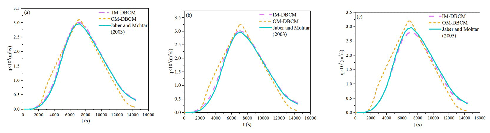
The hydrographs at the outlet node with coordinates of (500 m, 400 m) obtained from different models are shown in Fig. 7. A model proposed by Jaber and Mohtar (2003) was also used to simulate the overland runoff. Because finer grids and small time steps were used to divide the computational domain to obtain more accurate results in the model developed by Jaber and Mohtar (2003), the results calculated by Jaber and Mohtar (2003) can be used as a reference solution.

From Fig. 7, we can see that the IM-DBCM had a shape as well as a peak discharge close to the results simulated by Jaber and Mohtar (2003) in all cases. But the peak discharge of the hydrograph is slightly overestimated by the OM-DBCM, which may be attributed to the difference in the variable interpolation between the coarse and fine grids. In the OM-DBCM, variables at the interpolation interface were equal to those at the cell centre, which was then used to interpolate variables between the coarse and fine grids through shared and hanging nodes. This interpolation method had two drawbacks. Firstly, it is not reasonable to assume that the variables at the interpolation interface are equal to those at the cell centre, and the resulting error could increase as the grid size increases. Besides, compared with bilinear interpolation, the values at the hanging nodes are calculated by linear interpolation through shared nodes, which may result in relatively large errors. The results show that the method of interpolating variables between the coarse and fine grids by developing ghost cells proposed in this study has acceptable accuracy.

To quantitatively assess the performance of IM-DBCM, the root-mean square error (RMSE) of different cases was computed. The RMSEs of case12, case15 and case10 were $\mathrm{4.01}\times {\mathrm{10}}^{-\mathrm{4}}$, $\mathrm{7.85}\times {\mathrm{10}}^{-\mathrm{3}}$ and $\mathrm{3.25}\times {\mathrm{10}}^{-\mathrm{2}}$, respectively. It is shown that the error gradually increased with the increasing ratio of coarse to fine grids. The IM-DBCM may capture the shape of the hydrograph in case12 and case15, both in limbs and in peak discharge, but the peak discharge is slightly underestimated in case10. A possible explanation is that compared to the coarse grids, the fine grids were able to better capture the geometry of the channel cross-sections. High-resolution grids can better represent small-scale topographic features and flow passages (Hou et al., 2018); consequently, the simulation results for case12 and case15 are more satisfactory than those for case10. Similarly, the simulation accuracy of the OM-DBCM also gradually decreased with the increasing ratio of coarse to fine grids. Overall, the benefit of using the IM-DBCM for the flood simulations is evident.

3.2 V-shaped catchment

A 2D surface flow simulation was conducted over a V-shaped catchment to evaluate the performance of the IM-DBCM. The computational domain is symmetrically V-shaped, with two symmetrical hillslopes converging to form a channel in the central region. The riverbed slopes −0.05 on the left side and 0.05 on the right side. The channel bed has zero slope in the x direction and a slope of 0.02 in the y direction. The Manning coefficient is 0.015 on the hillslope and 0.15 on the main channel. Detailed dimensions and associated information pertaining to the V-shaped catchment are presented in Fig. 8. The total simulation time was 10 800 s, with a constant rainfall intensity of 10.8 mm h⁻¹ applied for 5400 s.

Figure 8 Geometry and size of the V-shaped catchment.

The IM-DBCM was used to simulate the 2D surface flow over the V-shaped domain. The computational basin was divided into coarse and fine grids based on the D-infinity algorithm. The size of the fine grids was 10 m × 10 m, whereas that of the coarse grids was 20 m × 20 m. The grid partition is presented in Fig. S2, where a V-shaped zone near the watershed outlet was discretized using fine grids, while the remaining areas were discretized using coarse grids.

Beside the HM2D model, the coupled Mike SHE and Mike 11 were also developed to simulate the surface flow under the same conditions. In the HM2D, the grid size was set to 10 m × 10 m. In the coupled Mike SHE and Mike 11 model runs, Mike SHE was used to simulate the rainfall–runoff on the hillslopes and the grid sizes were also 10 m × 10 m, while Mike 11 was used to simulate the runoff in the channel. Results were all compared to measured data.

The discharge hydrographs obtained from different models are shown in Fig. 9. This figure showed a close match between the measured data and the computed results obtained using the IM-DBCM. This indicated that the results were encouraging and the overall trend was captured well. The hydrographs obtained from the IM-DBCM were closer to the analytical solution when compared to the coupled Mike SHE and Mike 11. The weir flow equation was utilized to couple Mike SHE and Mike 11. Notably, only mass was transferred between the models, excluding momentum. However, mass and momentum were exchanged between the hillslopes and river channels. The IM-DBCM model ensured the conservation of both mass and momentum, resulting in simulated hydrographs that closely matched the analytical solutions.

Comparing the hydrographs generated by the 2D hydrodynamic model and IM-DBCM, the discharge hydrographs exhibited congruence for the discharge receding limb and peak discharge. However, the consistency of the hydrographs simulated by these two models was less pronounced for the rising limb. In the rising limb, the flow calculated using IM-DBCM was lower than that simulated using HM2D. The disparity in hydraulic behaviour between the hydrodynamic and hydrologic models explains the observed phenomenon. The HM2D consistently simulated the surface flow using the 2D hydrodynamic model; conversely, the hydrologic model was employed solely to simulate the flood processes when the upstream water level receded below the threshold established in IM-DBCM. In the hydrologic models that lack time-partial derivative terms, the current velocity was determined solely by the instantaneous water level gradient. This differs from the previous calculation method, which added the flux term to the velocity at the previous time step. Consequently, the velocity calculation in 2D hydrodynamic models deviated from the IM-DBCM.

Figure 9 Measured and simulated results obtained from different models.

3.3 Flood simulation in a natural watershed

The Goodwin Creek watershed located in Panola County, Mississippi, USA, is often selected as a benchmark to assess the capability of flood models because of sufficient available observed data. Drainage is westerly into Long Creek, which flows into the Yocona River, one of the main rivers of the Yazoo River, a tributary of the Mississippi River. The Goodwin Creek watershed covers an area of 21.3 km². The overall terrain gradually slopes from northeast to southwest, which is consistent with the trend of the main channel, and the elevation ranges from 71 to 128 m. The computational basin and bed elevations are shown in Fig. 10.

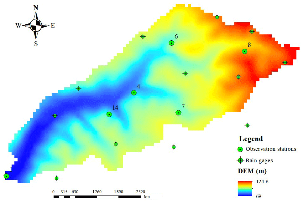
Figure 10 Overview of the Goodwin Creek watershed.

Land use in this watershed was divided into four classes including forest, water, cultivated and pasture, and their Manning coefficients were 0.05, 0.01, 0.03 and 0.04, respectively (Sánchez, 2002). The infiltration coefficients of different soil types were determined according to Blackmarr (1995). The rainfall event in 16 rain gauges (see Fig. 10) on 17 October 1981 was chosen for the simulation (Sánchez, 2002), and the inverse distance interpolation method (Barbulescu, 2016) was used to calculate the precipitation over the entire watershed. The rainfall duration was 4.8 h. Rainfall was spatially distributed at different times, as shown in Fig. S3. Data were measured at six observation stations (i.e. 1, 4, 6, 7, 8 and 14; Blackmarr, 1995), the locations of which are shown in Table S1 in the Supplement, and the simulated results were compared with the measured data from these stations.

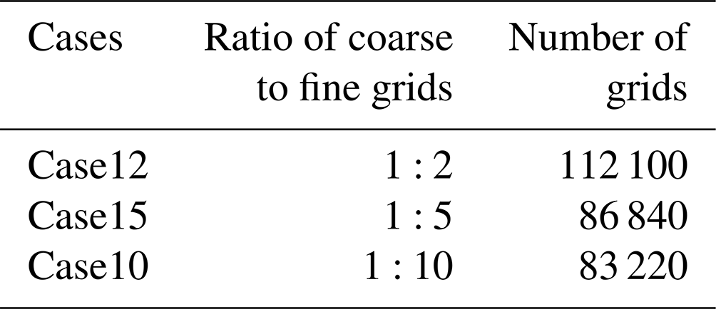
The simulations were performed for 12 h. Different cases with various grid resolutions were developed to verify the computational efficiency and numerical accuracy of IM-DBCM, as listed in Table 2. In M-DBCM, the rivers were covered by fine grid cells with dimensions of 10 m × 10 m, whereas the coarseness in the rest of the domain was increased to higher levels, as presented in Fig. S4.

Table 2 Different cases designed to simulate the Goodwin Creek watershed.

The OM-DBCM was also used to simulate the rainfall–runoff with the same resolutions. The Nash–Sutcliffe efficiency (NSE) was used to quantify errors in each model. The NSEs of IM-DBCM and OM-DBCM are shown in Table 3. From this table, we can see that the NSEs of IM-DBCM were higher than those of OM-DBCM at most stations, which was probably caused by the different interpolation method at the interface between coarse and fine grids. It is verified that the IM-DBCM has relatively high accuracy in simulating rainfall–runoff. In OM-DBCM, it is unreasonable to make the variables at the interface between coarse and fine grids equal to that at the cell centre, as this can bring errors. The induced error will increase as the ratio of coarse and fine grids increases. Therefore, it is also observed that the NSEs of OM-DBCM decreased with the increased ratio of coarse and fine grids. This indicated that the ghost cells and bilinear interpolation used in the IM-DBCM to interpolate variables between coarse and fine grids can make the simulation more reasonable.

Table 3 NSEs of different models (“IM” and “OM” refer to IM-DBCM and OM-DBCM, respectively).

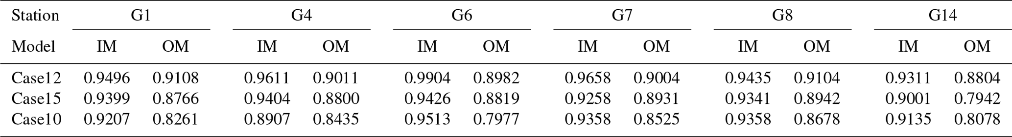
Figure 11 shows a comparison of the hydrographs measured and simulated by IM-DBCM at the monitoring gauges, the locations of which are presented in Fig. 10. At all gauges, the hydrographs obtained from different cases were aligned well with the measured data, which indicates that the IM-DBCM was able to reliably reproduce the flood wave propagation in the complex topography. The results of case12, in general, were better than those of case15 and case10, especially at station G1. A possible explanation is that a finer grid is needed to better capture the watershed geometry and obtain more satisfactory simulation accuracy. The cell sizes in case15 and case10 are larger than that in case12.

Figure 11 Hydrographs obtained from different cases.

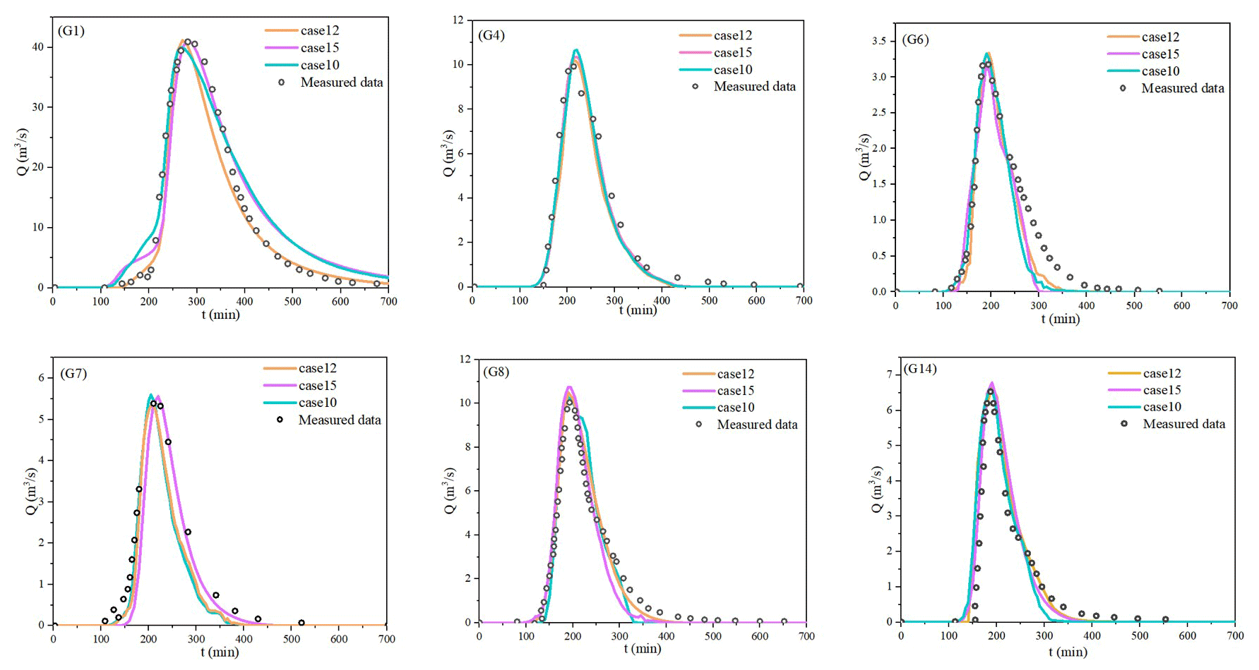
Compared to other stations, at station G1 the simulation results obtained from case15 and case10 deviated substantially from the measured data, especially the receding limb of the hydrographs. We deduced that the reason for this discrepancy is not the mesh partitioning but the location of G1. G1 is located at the watershed outlet, where water flows out of the watershed. The errors generated upstream may have accumulated at this station. Despite the deviation, the overall trend of the hydrographs indicated that the IM-DBCM is satisfactory and can reliably reproduce flood wave propagation in complex topography.

The water depth distribution at different times is shown in Fig. 12. The probability of flooding and inundation increases with increasing water depth. From 0 to 100 min, the water depth in the computational domain increased with the rainfall. The water depth across the computational domain is predominantly shallow, as shown in Fig. 12a. The discharge hydrographs within the watershed reached their peak at 200 min. The water depth in the watershed attained its maximum level concurrently, as shown in Fig. 12b. After 200 min, when rainfall stopped, the water depth in the computational watershed decreased (Fig. 12c).

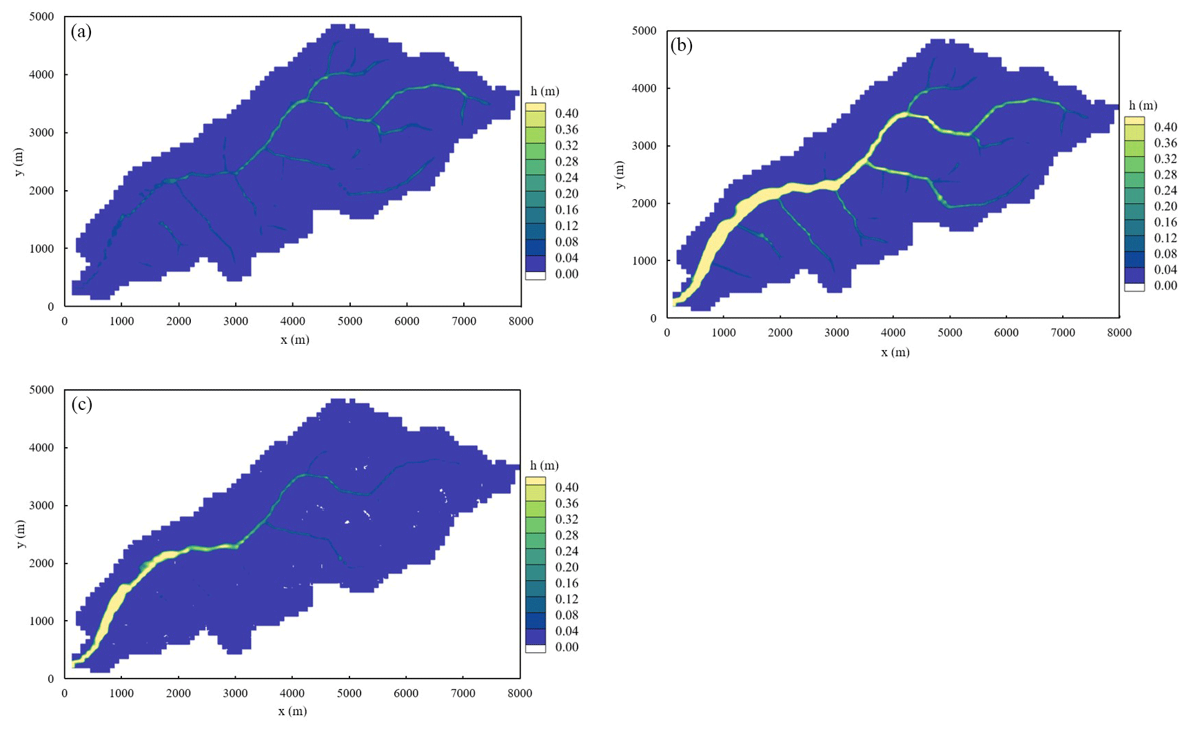
Figure 12 Water depth at different times. (a) t=100 min, (b) t=200 min, (c) t=400 min.

In terms of efficiency, the total execution time of IM-DBCM was compared to the uniform grid-based model (HM2D), as shown in Fig. 13. The total execution time of the different cases ranked from highest to lowest is as follows: HM2D > case12 > case15 > case10. Compared to HM2D, the multi-grid discrete computing domain improves computational efficiency by 60 %. Uniform fine grids were used to divide the computing zones in HM2D, and 207 198 computational grids were generated. Compared to HM2D, most of the areas were discretized with coarse grids, and only a small part of the region was calculated based on fine grids in IM-DBCM; the computational grids of the multi-grid-based model (Table 2) were considerably lower than those of HM2D. Furthermore, case12 required more computational time than case15 and case10. Fewer computational grid nodes were present in case15 and case10, which required less time for calculation, and the computational efficiency could be further improved. The advantages of using IM-DBCM based on multi-grids for flood simulations are evident. The difference in total runtime between the IM-DBCM and OM-DBCM is the time spent on mesh generation. In the OM-DBCM, the computational domain is divided manually, which is highly subjective, and the computational time varies from person to person.

However, there was not a significant difference in the computation time between case12, case15 and case10. The calculation time for coarse grids is shown in Fig. 13b. It was observed that the runtime for coarse grids decreases rapidly in different cases. In case12, case15 and case10, the number of coarse grids was 42 517, 7425 and 2153, respectively. As the number of coarse grids decreased significantly, the runtime for these grids also decreased rapidly. The number of fine grids is consistent in case12, case15 and case10, with a calculation time of 4800 s. The fine-grid number is much greater than that of the coarse grids, especially in case15 and case10. The 2D hydrodynamic model was solved in the fine-grid regions, which cost more computation time compared to the coarse grids where the hydrologic model was applied. The calculation time for fine grids is significantly longer than that for coarse grids, comprising a substantial portion of the overall execution time.

Figure 13 Computation time of different cases: (a) the relative differences between HM2D and IM-DBCM and (b) the runtime for coarse grids.

In many watersheds, the 2D inundation regions account for a minor proportion of the total watershed area. The fine grids were employed to partition the small inundation regions, while the coarse grids were utilized to discretize the majority of the non-inundation regions. The computational efficiency can be significantly enhanced due to the smaller proportion of fine grids and larger proportion of coarse grids. The IM-DBCM did not distinguish between the 1D rivers and 2D inundation regions, resulting in their division using fine grids. Consequently, the 2D hydrodynamic model was applied to both regions, leading to increased computational time. In future studies, the 1D hydrodynamic model will be used to compute the flood evolution specifically in the 1D rivers, leading to a reduction in computational time. Hence, the computational efficiency advantages of the proposed IM-DBCM are more pronounced.

4 Conclusions

An improved dynamic bidirectional coupled hydrologic–hydrodynamic model based on multi-grids (IM-DBCM) was presented in this study. A multi-grid system was generated based on the D-infinity algorithm, dividing regions that required high-resolution representation using fine grids from the rest requiring coarse grids to reduce computational load. A 2D nonlinear reservoir was adopted in the hydrologic model, while 2D shallow-water equations were applied in the hydrodynamic model. The hydrologic model was applied to the coarse-grid regions, whereas the hydrologic and hydrodynamic models were coupled in a bidirectional manner for the fine-grid areas. Different time steps were adopted in coarse and fine grids. Ghost cells and bilinear interpolation were used to interpolate variables between coarse and fine grids. The hydrologic and hydrodynamic models were dynamically and bidirectionally coupled with a time-dependent and moving coupling interface.

The performance of IM-DBCM was verified using three cases. The IM-DBCM was demonstrated to effectively simulate flow processes and ensure reliable simulation. Compared to the OM-DBCM, the results obtained from the IM-DBCM aligned well with the measured data, and it could reliably reproduce the flood wave propagation in complex topography. In addition to producing numerical results with similar accuracy, the IM-DBCM saved computational time compared to the model on fine grids. Furthermore, a moving coupling interface between the hydrologic and hydrodynamic models was observed in the IM-DBCM. The IM-DBCM has both high computational efficiency and high numerical accuracy and was adapted adequately to the real-life flooding process, providing practical and reliable solutions for rapid flood prediction and management, especially in large watersheds.

The IM-DBCM accurately and efficiently reproduces the flooding process and has the potential for a wide range of practical applications. The hydrologic model considers only surface runoff, which is appropriate for the intense rainfall-induced flood events examined in this study. However, a complete hydrologic model should include surface flow, interflow and underground runoff. In future works, the interflow and underground runoff could be calculated in the hydrologic model.