the Creative Commons Attribution 4.0 License.
the Creative Commons Attribution 4.0 License.
 | 23 May 2024
Simulating sea level extremes from synthetic low-pressure systems
Jani Räihä
Mika Rantanen
Matti Kämäräinen
In this article we present a method for numerical simulations of extreme sea levels using synthetic low-pressure systems as atmospheric forcing. Our simulations can be considered to be estimates of the high sea levels that may be reached when a low-pressure system of high intensity and optimal track passes the studied region. We test the method using sites located along the Baltic Sea coast and simulate synthetic cyclones with various tracks. To model the effects of the cyclone properties on sea level, we simulate internal Baltic Sea water level variations with a numerical two-dimensional hydrodynamic model, forced by an ensemble of time-dependent wind and air-pressure fields from synthetic cyclones. The storm surges caused by the synthetic cyclones come on top of the mean water level of the Baltic Sea, for which we used a fixed upper estimate of 100 cm. We find high extremes in the northern Bothnian Bay and in the eastern Gulf of Finland, where the sea level extreme due to the synthetic cyclone reaches up to 3.5 m. In the event that the mean water level of the Baltic Sea has a maximal value (1 m) during the cyclone, the highest sea levels of 4.5 m could thus be reached. We find our method to be suitable for use in further studies of sea level extremes.
- Article
(2781 KB) - Full-text XML
- BibTeX
- EndNote


A large part of the population and infrastructure in the Baltic Sea region is concentrated in the vicinity of the coastline. Therefore, it is crucial to consider the potential for extreme sea level conditions when ensuring the safety of citizens and implementing coastal flood protection measures. To quantify the coastal flooding risks, a comprehensive investigation of the present-day sea level variability and the possible scenarios for mean sea level in the future is essential (Pellikka et al., 2018, 2023; Leijala et al., 2018). As extremely high sea levels in the Baltic Sea are primarily caused by mid-latitude cyclones, the impact of atmospheric conditions on sea level extremes is an important research topic.
Sea level is measured by tide gauges situated on the coastline. For many locations on the Baltic Sea coast, tide gauge records are only available for the last 100–200 years, although historical floods can be reconstructed from other sources, e.g., historical records or studies of coastal sediments (Rutgersson et al., 2022). Nevertheless, it is possible that many sea level extremes of the last 1000 years have not left any traces in the historical record, especially in historically sparsely populated coastal areas such as around the coast of the Bothnian Bay. In addition, in the northern Baltic Sea, the coastline has retreated due to land uplift, and the coastal strip affected by flooding in the past is now further from the shore. Therefore, the effects of high sea levels have been reduced by the relative decrease in mean sea level with respect to the coastline.
The Baltic Sea is a shallow, semi-enclosed sea connected to the Atlantic Ocean through the narrow and shallow Danish straits. Local short-term variations in sea level are caused by winds, air pressure, currents, tides, and internal oscillations (seiches). Long-term changes are caused by global mean sea level variations, post-glacial land uplift, and the water flow between the North Sea and the Baltic Sea through the Danish straits (Leppäranta and Myrberg, 2009; Johansson et al., 2014). Sea level extremes in the Baltic Sea are the highest during the winter months, most commonly in November, December, and January (Wolski and Wiśniewski, 2023). These short-term sea level extremes (on hourly or daily timescales) are usually caused by moving extratropical cyclones, which in favorable atmospheric conditions can strengthen to powerful windstorms (Rantanen et al., 2024). Like sea level extremes, extratropical cyclones are most intense during the winter months, with about five windstorms per month in northern Europe (Laurila et al., 2021).
The effects of short-term sea level fluctuations are the largest in the narrow bays of the Baltic Sea. In particular, the narrow Gulf of Finland is vulnerable to coastal flooding due to windstorms, such as Storm Gudrun, which caused damage in 2005 (Tõnisson et al., 2008; Averkiev and Klevannyy, 2010). Major coastal flooding occurred in St. Petersburg in 1777, 1824, and 1924 (Kulikov and Medvedev, 2017), of which the 1824 flood was the most extreme, with a maximum sea level of 4.21 m. Even in cases where in situ sea level measurements are not available, traces of extreme sea level events can be found in sediment studies (Piotrowski et al., 2017; Leszczyńska et al., 2022). More information on sea level extremes in the Baltic Sea can be found in recent reviews considering the region (Weisse et al., 2021; Rutgersson et al., 2022).
The probabilities of extreme sea levels are usually estimated by applying extreme value analysis methods to observed sea level data (Arns et al., 2013). Extreme weather systems, such as tropical cyclones, rarely occur multiple times in a single location, so the extreme sea levels they cause are either unobserved or represented by single outliers. This makes it difficult to analyze extreme values of sea level data, especially in areas affected by tropical cyclones (O'Grady et al., 2022). However, even in the Baltic Sea, extratropical cyclones can cause extreme outliers in the statistics due to the shallow depth and shape of the coastline. For example, the highest sea level in the Gulf of Riga caused by Storm Gudrun in 2005 was an extreme outlier in the distribution (Mäll et al., 2017). Therefore, estimates of extremes based on statistical methods using observational data may be too conservative if cyclones caused by the highest sea level have not occurred at the location studied during the measurement period.
To overcome this limitation, studies have developed idealized low-pressure systems that can be used to investigate how high water levels could be caused by cyclones with optimal tracks and intensities in the Gulf of Finland (Averkiev and Klevannyy, 2010; Kalyuzhnaya et al., 2015; Apukhtin et al., 2017) and the Bothnian Bay (Gordeeva and Klevannyy, 2020). In a recent study (Andrée et al., 2022), synthetic uniform wind fields were used in extreme sea level simulations, and an empirical–statistical method was used to model the site-specific relationships between wind and extreme sea level. In addition, synthetic cyclones were used to assess the hazards of high sea level and waves in tropical regions (Leijnse et al., 2022; O'Grady et al., 2022).
In this study, we aim to estimate the highest plausible limits of extreme sea levels in the Baltic Sea caused by strong extratropical cyclones. To investigate how high sea levels could rise along the Baltic coast due to a storm with an optimal track, we reconstruct idealized cyclones that are physically realistic but have not occurred during the period of tide gauge observations. We describe the cyclones by a pressure field with a spatially varying time-dependent function that reproduces typical cyclone characteristics. The pressure and wind data are used as input into a numerical sea level model to simulate extreme sea levels.
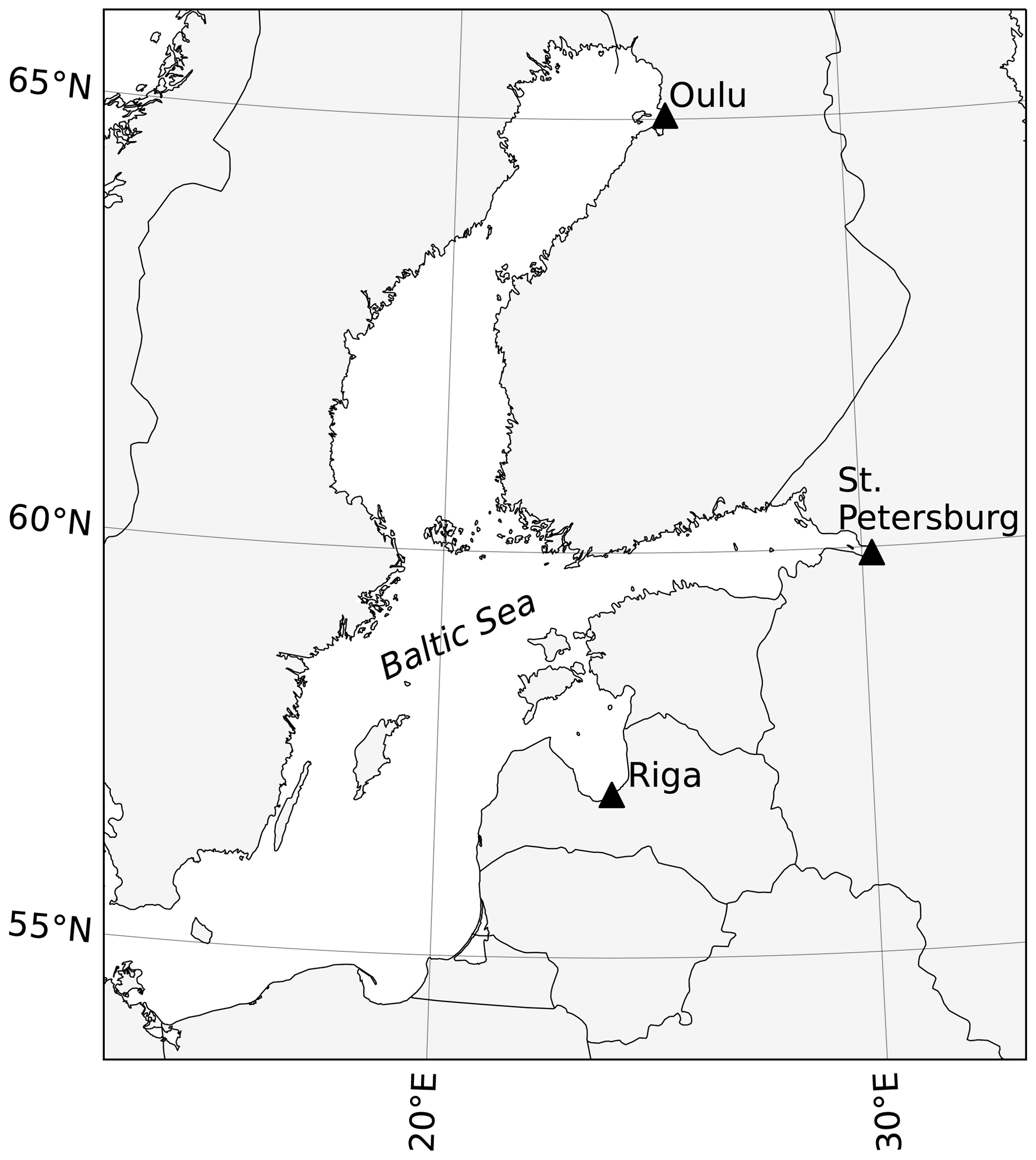
Figure 1The Baltic Sea and locations (Oulu, St. Petersburg, and Riga) where high sea levels were studied.
2.1 Synthetic atmospheric forcing
To model the sea levels associated with our synthetic cyclones, we need information on the atmospheric conditions for the forcing of the sea level model. To this end, we use a method where the mean sea level pressure and surface winds of the cyclone are calculated from the pressure field of a cyclone propagating with a constant velocity. The pressure field has the form of a Gaussian function
where P0 is the air pressure sufficiently far from the cyclone center; ΔP is the pressure anomaly in the cyclone center; x0 and y0 are the time-dependent coordinates of the cyclone center; and σ, the width of the pressure anomaly, is related to the radius R of the cyclone via σ=0.25 R. The 10 m geostrophic wind components (ug, vg) are calculated from the pressure field using the geostrophic balance as
where ug (m s−1) is the zonal geostrophic wind component, vg (m s−1) is the meridional geostrophic wind component, f=2Ωsin (ϕ) is the Coriolis parameter (Ω is the rotation rate of the Earth, and ϕ is the latitude), and ρ is the density of air (1.3 kg m−3). An example of the pressure and wind field of a synthetic cyclone is shown in Fig. 2.
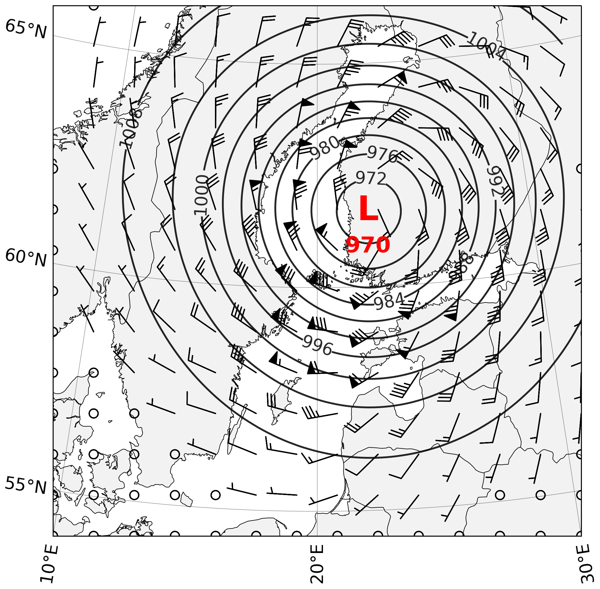
Figure 2Example of synthetic cyclone and induced winds. The contours represent sea level pressure (hPa), and the wind barbs represent 10 m winds (knots).
Actual wind components (u, v) differ from the geostrophic winds (ug, vg), especially near the surface where friction acts to slow winds down, leading to winds turning counterclockwise in the Northern Hemisphere, and where curvature effects (the centrifugal force) are important. We study this difference between the theoretical geostrophic and the actual near-surface wind by using the analysis previously applied by Särkkä et al. (2017), with linear regression applied separately for wind speed and direction in the ERA-Interim reanalysis dataset (Dee et al., 2011) over the 1979–2012 period. We obtain spatially varying coefficients for wind speed and direction change by comparing the actual 10 m winds of the reanalysis dataset with geostrophic winds that we calculate from the mean sea level pressure field. We then modify the geostrophic winds in the cyclone generator with coefficients from Särkkä et al. (2017) to achieve more realistic wind fields. Finally, we save these wind fields and pressure fields in a numerical grid and use them as the input of the sea level model.
2.2 Limitations of the synthetic cyclone
It should be noted that the use of synthetic cyclones is inevitably subject to certain limitations. One of these is the Gaussian shape of the cyclone. As can be seen from Fig 2, the spatial field of the simulated cyclone is not entirely realistic, as the cyclone is symmetrical and lacks the frontal structures typical of extratropical cyclones. However, the Gaussian shape was originally chosen for two main reasons: (1) it requires only two parameters to describe it, and (2) it describes the general shape of cyclones with sufficient accuracy. It is clear, of course, that not all possible variations in cyclone shape can be described by the Gaussian simplification. However, we would like to emphasize the importance of other factors in determining sea level variations. For example, far more relevant to simulated sea levels than the deviations of the shapes from Gaussian are (1) the depth and extent of the cyclone and (2) the track and propagation speed of the cyclone.
Furthermore, the pressure anomaly of the simulated cyclone is not time dependent, neglecting the deepening and filling of the cyclone. The value of the pressure anomaly affects the simulated sea level mainly when the cyclone moves over the sea. In the Baltic Sea, the cyclone passes the sea area in less than 24 h, limiting the effect of the time-varying pressure anomaly on the simulated coastal sea level.
2.3 Cyclone parameters
The horizontal extent and depth of the synthetic cyclone, related to the radius R and ΔP, must be limited by physical considerations. According to Rudeva and Gulev (2007), the effective radius of cyclones over the ocean can be greater than 900 km, with an average of about 700 km. Therefore, we set the radius R to 1000 km, although we acknowledge that this value may be at the upper limit of what is plausible in the Baltic Sea region (Rudeva and Gulev, 2007).
The pressure anomaly ΔP was constrained by the resulting geostrophic wind speeds. Based on observations and previous work, we decided that surface mean wind speeds should not exceed 40 m s−1. This limit roughly corresponds to the maximum wind speeds observed during Storm Gudrun (mean wind speed 33 m s−1, wind gust 42 m s−1, Valinger and Fridman, 2011, and 40 m s−1 was also the highest stationary wind speed examined in a recent study of wind-driven extreme sea levels, Andrée et al., 2022). With this constraint, the pressure anomaly ΔP was set to −40 hPa.
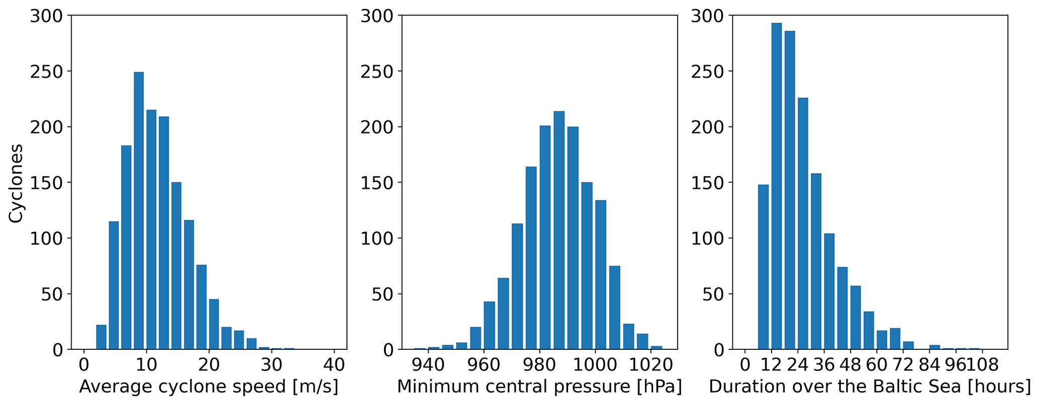
Figure 3Distribution of mean speeds, minimum pressures and durations of cyclones that pass the Baltic Sea region in October–March 1979–2020 in ERA5 reanalysis.
The numerical sea level model describes how surface winds cause water flow through the wind friction component in the Navier–Stokes equations. The dependence of the wind friction on velocity is quadratic in our model, but in reality this dependence is likely different for extreme wind speeds (over 50 m s−1). This is an additional argument for limiting the surface wind speeds to 40 m s−1 for the synthetic cyclones. We fix the radius of the cyclone and the pressure anomaly using the values mentioned above (which also limits wind speeds) and vary four parameters in the simulations: the latitude and longitude of cyclone origin plus the speed and direction of cyclone propagation (cyclone velocity and direction given by zonal speed u and meridional speed v). We estimate the distribution of mean cyclone velocities for storms that pass the Baltic Sea region during October–March 1979–2020 based on ERA5 reanalysis data (Hersbach et al., 2020) using the same cyclone track dataset as was used in Laurila et al. (2021). The smallest velocities from this analysis are around 5 m s−1 (Fig. 3a). Even smaller velocities of the cyclone lead to situations where the cyclone is almost stationary, with cyclone winds piling water towards the coast. As this scenario is likely unrealistic, we limit the minimum velocity of the cyclone to 5 m s−1.
2.4 Numerical sea level simulation
In our numerical simulations we use a barotropic sea level model which describes the internal (intra-basin) fluctuations of the Baltic Sea with a set of two-dimensional hydrodynamic equations (Häkkinen, 1980). These equations are based on shallow-water equations, derived from the Navier–Stokes equations by integrating the vertical coordinate out. Surface winds and surface pressure are used as atmospheric forcing for the sea level model. The computational domain extends from 53 to 66° N and from 9 to 31° E. The spacing of the numerical grid is 0.1° in the meridional direction and 0.2° in the zonal direction. We treat the Baltic Sea as a closed basin, with no connection through the Danish straits to the North Sea. The model has previously been validated with Finnish tide gauge data and with ERA-Interim forcing for 1979–2012 (Särkkä et al., 2017). The correlation between hourly data of simulated and observed sea levels was from 0.91 to 0.94 for all 13 Finnish tide gauge sites, even if the spacing of the numerical grid was sparser (0.25×0.5°) than in this study. The details of the sea level model were explained in Särkkä et al. (2017).
The variations in the water volume of the Baltic Sea are mainly caused by the flow of the water in and out of the Baltic Sea through the Danish straits. The contribution of the water volume to the local sea level (also called preconditioning) is termed the water balance component. This component can be estimated with a statistical model, based on wind speeds at a single coordinate point at 55° N and 15° E (Johansson et al., 2014; Särkkä et al., 2017). The progression of a cyclone over the Baltic Sea region in the high-sea-level cases takes only 1 or 2 d, and the change in the water balance within this time is small (less than 10 cm). Thus we do not include changes in the water balance in our simulations. Instead, we estimate the extreme value of the water balance component to be 100 cm (Särkkä et al., 2017) and add it to the simulated local sea level maximum. This describes the situation when preceding weather conditions have raised the water volume in the Baltic Sea, and then the arriving cyclone causes fluctuations on top of the high mean sea level.
The tides are small in the Baltic Sea, with the largest tidal ranges (over 20 cm) at the eastern end of the Gulf of Finland and near the Danish straits in the southwestern Baltic Sea. For a large part of the Baltic coast, the tidal range is only a few centimeters (Medvedev et al., 2016), and thus we do not include tides in the model.
2.5 Simulation parameters
As we are interested in the highest sea levels on the Baltic Sea coast, we select three sites to represent different bay areas of the Baltic Sea, including coastal cities where the sea level variability is large and where the effects of flooding are significant – the latter due to dense inhabitation with substantial infrastructure on low-lying coastlines. As the predominant direction of the cyclone tracks is from the west, we choose to study sites at the ends of bays, on the eastern coast of the Baltic Sea. At these locations, the effect of wind-driven water transport is large, as the water piles towards the coastline. We select the locations so that the Gulf of Bothnia is represented by Oulu, situated at its northern end (Fig. 1). The Gulf of Finland is represented by St. Petersburg, situated at its eastern end. The smaller sub-basin, the Bay of Riga, is represented by Riga. In the Gulf of Bothnia, we also simulated sea levels at Kemi but found that the highest simulated sea levels at Oulu exceeded the ones found at Kemi.
We use the surface wind and pressure fields of synthetic cyclones as atmospheric forcing for the sea level model. We compare simulation results with the observed extremes in tide gauge data from Fig. 1 of Averkiev and Klevannyy (2010). As the initial condition for the Baltic Sea level in the simulation is a uniform constant sea level, our results represent the sea level fluctuation with respect to the prevailing mean sea level in the Baltic Sea preceding the arrival of the cyclone.
To compare the simulated extremes for different locations with the observed ones, we add 100 cm to the simulated extreme, which takes into account the high water volume in the Baltic Sea that often prevails before the extreme sea level situation. As our aim is only to estimate the local extremes to an accuracy of tens of centimeters, we use a fixed value of 100 cm for the initial sea level for all simulated sites with respect to the reference level, even if this level differs between the national vertical reference systems used for different sites.
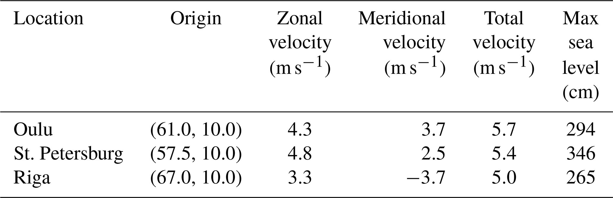
In Table 1 we give the parameters that yield the highest sea levels at each of the three sites. The origins of the cyclones are all on the longitude 10° E. The effect of the winds on the sea level fluctuation with the distance close to the radius from the cyclone center is small; thus it was found that it is not necessary to set the cyclone origin further in the west. A common factor for the cyclone tracks of these maxima was that the propagation speeds were close to the minimum speed limit 5.0 m s−1:5.7 m s−1 for Oulu, 5.4 m s−1 for St. Petersburg, and 5.0 m s−1 for Riga. Due to the low propagation speed, high wind speeds prevail for a longer time over the Baltic Sea, enhancing the water flow towards the ends of bays.
Table 1Cyclone parameters for the highest simulated sea levels at Oulu, St. Petersburg, and Riga.
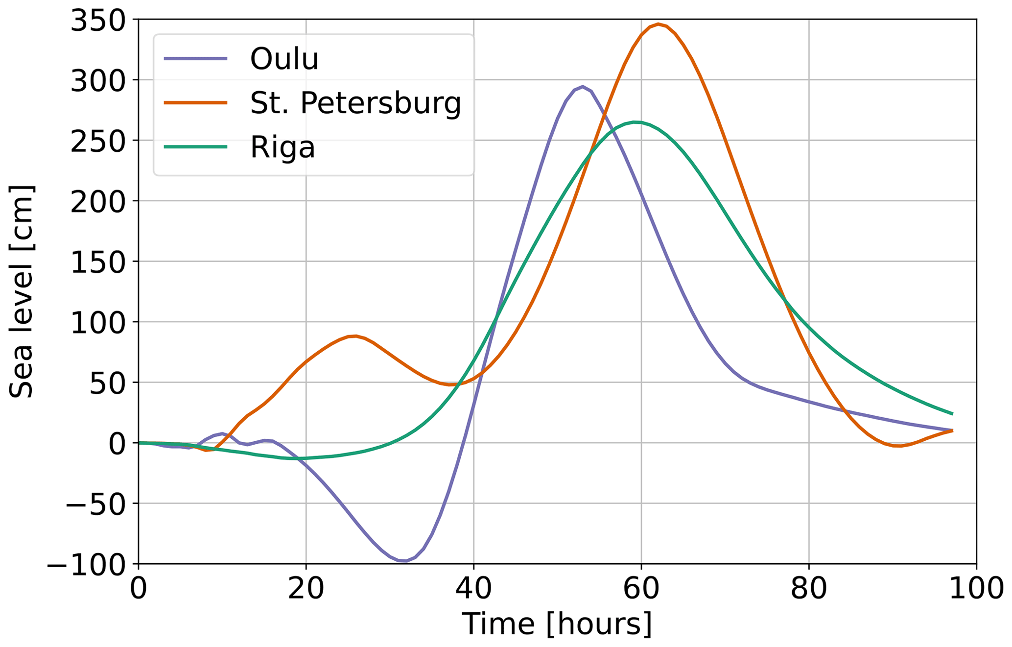
The simulated sea level extreme at Oulu is caused by a cyclone progressing northeastwards from southern Norway towards Finnish Lapland (Fig. 4). The strong winds on the right-hand side of the propagation direction generate water flow from the central Baltic Sea towards the northern end of the Bothnian Bay. At first, the wind direction in front of the cyclone center is towards the northwest in the Bothnian Bay, moving water away from Oulu and causing a decrease in sea level down to −100 cm. Then, as the cyclone center moves northwest of the Bothnian Bay, the wind direction is towards the northeast, piling water towards the northeastern end of the bay, which causes a rapid increase in sea level at Oulu. Finally, when the cyclone is north of the Bothnian Bay, the wind direction is from west to east over the northern Bothnian Bay. This pushes yet more water towards the Oulu coastal region, leading to a very high sea level maximum of 294 cm (Fig. 5). The highest observed sea level at Oulu is 183 cm from 14 January 1984. This event was caused by a deep low pressure (950 hPa) having its center in Sweden, inducing southern winds that both increased the water amount in the Baltic Sea and pushed water towards the end of the Bothnian Bay. Taking into account the maximum water balance component (100 cm), a sea level at Oulu of 394 cm could be reached, which is significantly higher than the observed maximum value. In the study of Andrée et al. (2022) with uniform wind fields (wind speed 22 m s−1), the highest simulated sea levels in the Bothnian Bay were at Kalix and Kemi (both situated west of Oulu), where extreme sea levels between 275 and 300 cm were obtained. These levels are of the same magnitude as our result for the extreme sea level at Oulu without the water balance component.
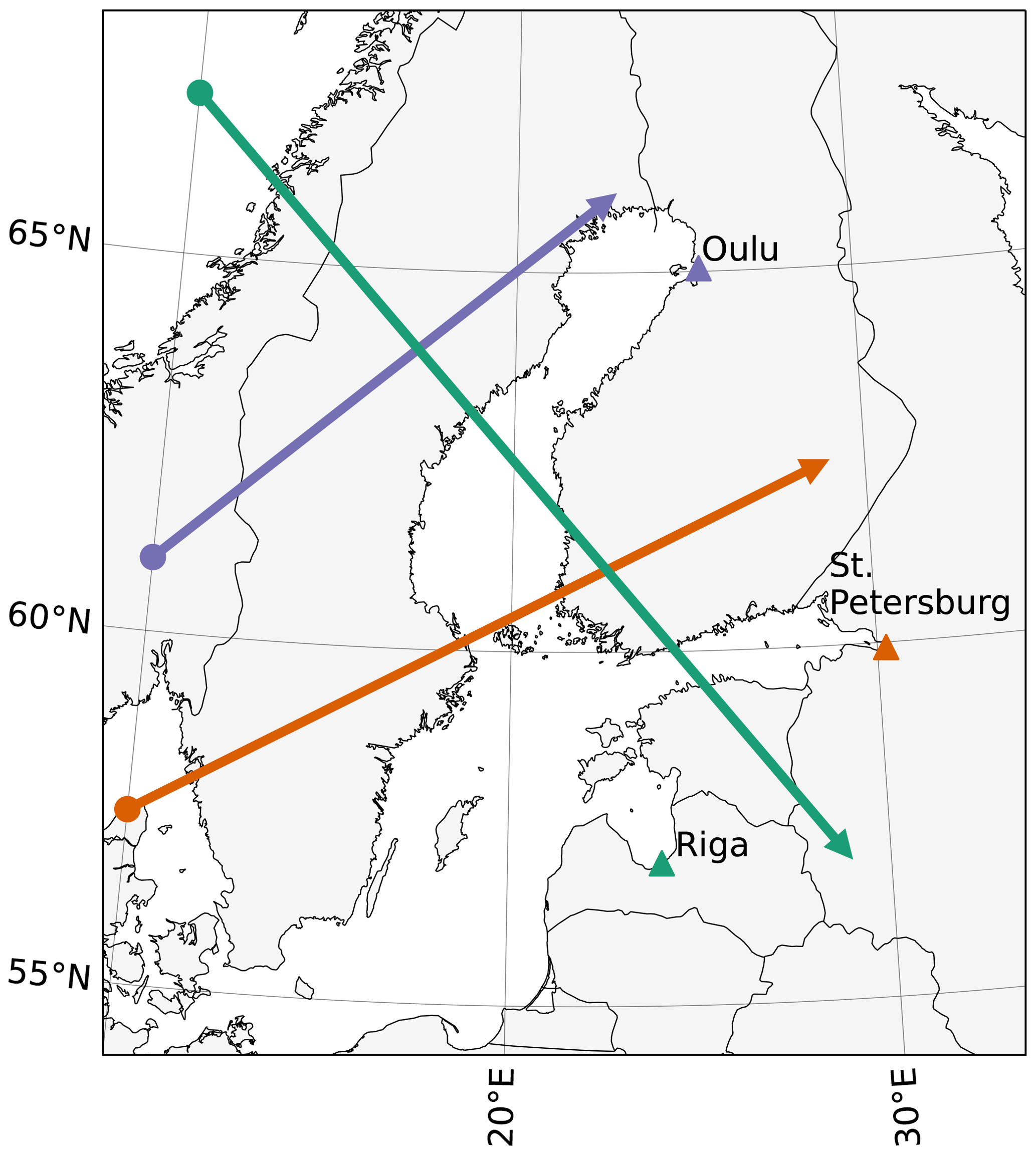
Figure 4Cyclone tracks of the highest simulated sea levels at Oulu, St. Petersburg, and Riga.
Räty et al. (2023) used Bayesian hierarchical modeling to analyze return level estimates and theoretical upper limits for the sea level on the Finnish coast from tide gauge data. At Oulu, the 1000-year return level is approximately 200 cm, and the theoretical upper limit for the sea level using Bayesian modeling is approximately 250 cm. These estimates include the water balance component and are considerably lower than the nearly 4 m estimate in our analysis. This indicates that the high values that we obtain from our synthetic cyclone method can not always be derived from the statistical extreme value analysis.
The cyclone track that causes the highest simulated sea level extreme at St. Petersburg (346 cm, Fig. 4) is interesting. The cyclone enters the Baltic Sea region from northern Denmark and moves over southern Finland. Winds cause water to flow from the central Baltic Sea to the Gulf of Finland, which accumulates water at its eastern end. The highest observed sea level occurred in 1824, reaching 421 cm at St. Petersburg. In the study of Averkiev and Klevannyy (2010), the pressure anomaly was a time-dependent exponential function, having a maximum pressure anomaly −50 hPa and a minimum pressure 960 hPa at 61.7° N and 29.0° E. The maximum wind speed in the Gulf of Finland was 41 m s−1, and the velocity of the cyclone was 14.24 m s−1. The initial position of the cyclone center was at 60° N and 10° E, and the cyclone track crossed 30° E at the Finnish–Russian border. In our simulation (Fig. 4), the initial position is more southern (57.5° N, 10° E), but the crossing of 30° E is north of the track of the cyclone in Averkiev and Klevannyy (2010), and the velocity is slower (5.4 m s−1). The simulated sea level at St. Petersburg by Averkiev and Klevannyy (2010) was 590 cm, where the initial mean sea level was set to 0 cm. The rapid deepening of the pressure anomaly over the Gulf of Finland leads to this extreme value in Averkiev and Klevannyy (2010), whereas in our simulation the piling up of water in the end of the Gulf of Finland is the main factor in the extreme sea level of 346 cm. Taking into account the maximum water volume of the Baltic Sea by adding 100 cm, the highest estimated sea level in our simulations at St. Petersburg is 446 cm. The narrow shape of the Gulf of Finland and its west–east orientation leave the eastern end of the Gulf of Finland especially vulnerable to sea flooding when weather conditions induce water transport towards St. Petersburg.
The highest simulated sea level maximum at Riga is due to a cyclone approaching from central Norway, then moving to the southeast over the Bothnian Sea and southwestern Finland (Fig. 4). Northerly winds push water from the Bothnian Sea and central Baltic Sea towards the Bay of Riga. As the cyclone moves over the Gulf of Finland and Estonia to Russia, the northwesterly winds cause water accumulation in the vicinity of Riga. The simulated maximum at Riga is 265 cm. The highest observed sea level is 229 cm from November 1969. By adding the water balance component of 100 cm, the highest estimated sea level is 365 cm, considerably higher than the observed maximum.
In summary, the simulated extremes clearly exceed the observed ones at Oulu and Riga, even accounting for a tens of centimeters ambiguity in the value of the water balance component from the reference level of the tide gauge location. At St. Petersburg, however, the simulated extreme is of similar height to the observed extreme in 1824.
The results of our study show that a numerical sea level model combined with synthetic cyclones can be used to study the characteristics of cyclones that induce extreme sea levels on the Baltic coast. Comparing the three studied sites, we find the highest simulated sea levels at St. Petersburg – around 3.5 m – so that, adding the water balance component, sea levels over 4 m are possible. These values are comparable with the values observed during the extreme flood of 1824 (421 cm in St. Petersburg). As the flood in 1824 was the highest in the 300-year history of St. Petersburg, the simulated case could correspond to the extreme weather conditions that contributed to the sea levels observed in 1824.
The high sea level at Oulu, approximately 4.0 m, is due to a cyclone causing water flow from the entire Gulf of Bothnia towards the northern Bothnian Bay and finally the change in wind direction from westwards to eastwards in the Bothnian Bay. One could expect that an even higher sea level would be found in Kemi, situated at the northern end of the Bothnian Bay, as the highest sea level in Finland (201 cm in 1982) was observed there. In our simulations at Kemi (results not discussed in this publication), the highest maxima are all under 4.0 m. The shape of the coastline and bathymetry in the Bothnian Bay apparently favor high sea levels at Oulu more than at Kemi. Our simulation results indicate that there is potential for a flood exceeding 4 m at Oulu, far surpassing the observed maximum in 1984 (183 cm).
At Riga, the highest simulated sea level is obtained with a cyclone passing the Baltic Sea with a track from central Sweden towards northwestern Russia. The simulated extreme of 265 cm (with 1 m added to include the water balance component) is considerably higher than the observed maximum (229 cm) in 1969. The cyclone related to the maximum in 1969 had a similar track compared to the one used in our simulation. This indicates that a similar storm track can occur and that a cyclone with such a track and slow velocity could cause high sea levels in the Riga region.
The effect of waves on the extreme sea levels on the coast was not considered in this study, as this effect strongly depends on the bathymetry and on the location. Our aim was not to rigorously evaluate the highest sea level taking into account all factors but to evaluate what the contribution of the synthetic cyclone is to the sea level maximum, which already exceeds observed sea level extremes in many locations on the Baltic Sea coast. For detailed studies of extreme sea levels for a single site, simultaneous sea level and wave simulations are needed, and such studies have already been conducted in the Baltic Sea (Apukhtin et al., 2017; Gordeeva and Klevannyy, 2020).
Our results indicate that synthetic cyclones are a useful tool for studying the sea level response to cyclones with different characteristics. In particular, our method offers the opportunity to study the extreme sea levels which can be expected on the Baltic Sea coast if all the components that raise the water level are present, namely a high water balance paired with a slow and deep cyclone moving along an optimal track. Our simulations of extreme sea levels reveal the areas of the Baltic Sea which, due to shoreline geometry and coastal bathymetry, are especially prone to extreme coastal flooding.
Code for reproducing the synthetic cyclones of this study has been made publicly available in Zenodo https://doi.org/10.5281/zenodo.11242301 (Räihä and Kämäräinen, 2024).
The package contains the Python code for creating the cyclones with the necessary input files. The output of the code is the wind and pressure data of the synthetic cyclone.
All authors contributed to the design of the study. JR and MK implemented the method for the generation of synthetic cyclones. JS implemented the numerical sea level model. MR studied the properties of cyclones from reanalysis data. JS performed the sea level simulations with synthetic cyclones, conducted the analysis presented in the paper, and wrote the paper with critical comments from the other authors.
The contact author has declared that none of the authors has any competing interests.
Publisher's note: Copernicus Publications remains neutral with regard to jurisdictional claims made in the text, published maps, institutional affiliations, or any other geographical representation in this paper. While Copernicus Publications makes every effort to include appropriate place names, the final responsibility lies with the authors.
The authors thank the two anonymous reviewers for their constructive comments, which helped to improve the paper.
This research has been supported by the Finnish State Nuclear Waste Management Fund (VYR) through the Finnish Research Programme on Nuclear Power Plant Safety 2019–2022 (SAFIR2022).
This paper was edited by Rachid Omira and reviewed by two anonymous referees.
Andrée, E., Drews, M., Su, J., Larsen, M. A. D., Drønen, N., and Madsen, K. S.: Simulating wind-driven extreme sea levels: Sensitivity to wind speed and direction, Weather Clim. Extrem., 36, 100422, https://doi.org/10.1016/j.wace.2022.100422, 2022. a, b, c
Apukhtin, A., Bessan, G., Gordeeva, S., Klevannaya, M., and Klevannyy, K.: Simulation of the probable maximum flood in the area of the Leningrad Nuclear Power Plant with account of wind waves, Russ. Meteorol. Hydrol., 42, 113–120, 2017. a, b
Arns, A., Wahl, T., Haigh, I., Jensen, J., and Pattiaratchi, C.: Estimating extreme water level probabilities: A comparison of the direct methods and recommendations for best practise, Coast. Eng., 81, 51–66, https://doi.org/10.1016/j.coastaleng.2013.07.003, 2013. a
Averkiev, A. S. and Klevannyy, K. A.: A case study of the impact of cyclonic trajectories on sea-level extremes in the Gulf of Finland, Cont. Shelf Res., 30, 707–714, https://doi.org/10.1016/j.csr.2009.10.010, 2010. a, b, c, d, e, f, g
Dee, D. P., Uppala, S. M., Simmons, A. J., Berrisford, P., Poli, P., Kobayashi, S., Andrae, U., Balmaseda, M. A., Balsamo, G., Bauer, P., Bechtold, P., Beljaars, A. C. M., van de Berg, L., Bidlot, J., Bormann, N., Delsol, C., Dragani, R., Fuentes, M., Geer, A. J., Haimberger, L., Healy, S. B., Hersbach, H., Hólm, E. V., Isaksen, L., Kållberg, P., Köhler, M., Matricardi, M., McNally, A. P., Monge-Sanz, B. M., Morcrette, J.-J., Park, B.-K., Peubey, C., de Rosnay, P., Tavolato, C., Thépaut, J.-N., and Vitart, F.: The ERA-Interim reanalysis: configuration and performance of the data assimilation system, Q. J. Roy. Meteorol. Soc., 137, 553–597, https://doi.org/10.1002/qj.828, 2011. a
Gordeeva, S. M. and Klevannyy, K. A.: Estimation of the maximum and minimum surge levels at the Hanhikivi peninsula, Gulf of Bothnia, Boreal Environ. Res., 25, 51–63, 2020. a, b
Häkkinen, S.: Computation of sea level variations during December 1975 and 1 to 17 September 1977 using numerical models of the Baltic Sea, Deutsche Hydrographische Zeitschrift, 33, 158–175, 1980. a
Hersbach, H., Bell, B., Berrisford, P., Hirahara, S., Horányi, A., Muñoz-Sabater, J., Nicolas, J., Peubey, C., Radu, R., Schepers, D., Simmons, A., Soci, C., Abdalla, S., Abellan, X., Balsamo, G., Bechtold, P., Biavati, G., Bidlot, J., Bonavita, M., De Chiara, G., Dahlgren, P., Dee, D., Diamantakis, M., Dragani, R., Flemming, J., Forbes, R., Fuentes, M., Geer, A., Haimberger, L., Healy, S., Hogan, R. J., Hólm, E., Janisková, M., Keeley, S., Laloyaux, P., Lopez, P., Lupu, C., Radnoti, G., de Rosnay, P., Rozum, I., Vamborg, F., Villaume, S., and Thépaut, J.-N.: The ERA5 global reanalysis, Q. J. Roy. Meteorol. Soc., 146, 1999–2049, https://doi.org/10.1002/qj.3803, 2020. a
Johansson, M. M., Pellikka, H., Kahma, K. K., and Ruosteenoja, K.: Global sea level rise scenarios adapted to the Finnish coast, J. Mar. Syst., 129, 35–46, https://doi.org/10.1016/j.jmarsys.2012.08.007, 2014. a, b
Kalyuzhnaya, A. V., Visheratin, A. A., Dudko, A., Nasonov, D., and Boukhanovsky, A. V.: Synthetic storms reconstruction for coastal floods risks assessment, J. Comput. Sci., 9, 112–117, https://doi.org/10.1016/j.jocs.2015.04.029, 2015. a
Kulikov, E. A. and Medvedev, I. P.: Extreme Statistics of Storm Surges in the Baltic Sea, Oceanology, 57, 772–783, https://doi.org/10.1134/S0001437017060078, 2017. a
Laurila, T. K., Gregow, H., Cornér, J., and Sinclair, V. A.: Characteristics of extratropical cyclones and precursors to windstorms in northern Europe, Weather Clim. Dynam., 2, 1111—1130, https://doi.org/10.5194/wcd-2-1111-2021, 2021. a, b
Leijala, U., Björkqvist, J.-V., Johansson, M. M., Pellikka, H., Laakso, L., and Kahma, K. K.: Combining probability distributions of sea level variations and wave run-up to evaluate coastal flooding risks, Nat. Hazards Earth Syst. Sci., 18, 2785–2799, https://doi.org/10.5194/nhess-18-2785-2018, 2018. a
Leijnse, T. W. B., Giardino, A., Nederhoff, K., and Caires, S.: Generating reliable estimates of tropical-cyclone-induced coastal hazards along the Bay of Bengal for current and future climates using synthetic tracks, Nat. Hazards Earth Syst. Sci., 22, 1863–1891, https://doi.org/10.5194/nhess-22-1863-2022, 2022. a
Leppäranta, M. and Myrberg, K.: Physical Oceanography of the Baltic Sea, Springer, https://doi.org/10.1007/978-3-540-79703-6, 2009. a
Leszczyńska, K., Stattegger, K., Moskalewicz, D., Jagodziński, R., Kokociński, M., Niedzielski, P., and Szczuciński, W.: Controls on coastal flooding in the southern Baltic Sea revealed from the late Holocene sedimentary records, Sci. Rep., 12, 9710, https://doi.org/10.1038/s41598-022-13860-4, 2022. a
Mäll, M., Suursaar, Ü., Nakamura, R., and Shibayama, T.: Modelling a storm surge under future climate scenarios: case study of extratropical cyclone Gudrun (2005), Nat. Hazards, 89, 1119–1144, 2017. a
Medvedev, I. P., Rabinovich, A. B., and Kulikov, E. A.: Tides in Three Enclosed Basins: The Baltic, Black, and Caspian Seas, Front. Mar. Sci., 3, 46, https://doi.org/10.3389/fmars.2016.00046, 2016. a
O'Grady, J. G., Stephenson, A. G., and McInnes, K. L.: Gauging mixed climate extreme value distributions in tropical cyclone regions, Sci. Rep., 12, 4626, https://doi.org/10.1038/s41598-022-08382-y, 2022. a, b
Pellikka, H., Leijala, U., Johansson, M. M., Leinonen, K., and Kahma, K. K.: Future probabilities of coastal floods in Finland, Cont. Shelf Res., 157, 32–42, https://doi.org/10.1016/j.csr.2018.02.006, 2018. a
Pellikka, H., Johansson, M. M., Nordman, M., and Ruosteenoja, K.: Probabilistic projections and past trends of sea level rise in Finland, Nat. Hazards Earth Syst. Sci., 23, 1613–1630, https://doi.org/10.5194/nhess-23-1613-2023, 2023. a
Piotrowski, A., Szczuciński, W., Sydor, P., Kotrys, B., Rzodkiewicz, M., and Krzymińska, J.: Sedimentary evidence of extreme storm surge or tsunami events in the southern Baltic Sea (Rogowo area, NW Poland), Geol. Quart., 61, 973–986, https://doi.org/10.7306/gq.1385, 2017. a
Räihä, J. and Kämäräinen, M.: Supplementary Python code and related files, Zenodo [code], https://doi.org/10.5281/zenodo.11242301, 2024. a
Rantanen, M., van den Broek, D., Cornér, J., Sinclair, V. A., Johansson, M. M., Särkkä, J., Laurila, T. K., and Jylhä, K.: The Impact of Serial Cyclone Clustering on Extremely High Sea Levels in the Baltic Sea, Geophys. Res. Lett., 51, e2023GL107203, https://doi.org/10.1029/2023GL107203, 2024. a
Räty, O., Laine, M., Leijala, U., Särkkä, J., and Johansson, M. M.: Bayesian hierarchical modeling of sea level extremes in the Finnish coastal region, Nat. Hazards Earth Syst. Sci., 23, 2403–2418, https://doi.org/10.5194/nhess-23-2403-2023, 2023. a
Rudeva, I. and Gulev, S. K.: Climatology of cyclone size characteristics and their changes during the cyclone life cycle, Mon. Weather Rev., 135, 2568–2587, https://doi.org/10.1175/MWR3420.1, 2007. a, b
Rutgersson, A., Kjellström, E., Haapala, J., Stendel, M., Danilovich, I., Drews, M., Jylhä, K., Kujala, P., Larsén, X. G., Halsnæs, K., Lehtonen, I., Luomaranta, A., Nilsson, E., Olsson, T., Särkkä, J., Tuomi, L., and Wasmund, N.: Natural hazards and extreme events in the Baltic Sea region, Earth Syst. Dynam., 13, 251–301, https://doi.org/10.5194/esd-13-251-2022, 2022. a, b
Särkkä, J., Kahma, K. K., Kämäräinen, M., Johansson, M. M., and Saku, S.: Simulated extreme sea levels at Helsinki, Boreal Environ. Res., 22, 299–315, 2017. a, b, c, d, e, f
Tõnisson, H., Orviku, K., Jaagus, J., Suursaar, Ü., Kont, A., and Rivis, R.: Coastal Damages on Saaremaa Island, Estonia, Caused by the Extreme Storm and Flooding on January 9, 2005, J. Coast. Res., 24, 602–614, https://doi.org/10.2112/06-0631.1, 2008. a
Valinger, E. and Fridman, J.: Factors affecting the probability of windthrow at stand level as a result of Gudrun winter storm in southern Sweden, Forest Ecol. Manage., 262, 398–403, 2011. a
Weisse, R., Dailidienė, I., Hünicke, B., Kahma, K., Madsen, K., Omstedt, A., Parnell, K., Schöne, T., Soomere, T., Zhang, W., and Zorita, E.: Sea level dynamics and coastal erosion in the Baltic Sea region, Earth Syst. Dynam., 12, 871–898, https://doi.org/10.5194/esd-12-871-2021, 2021. a
Wolski, T. and Wiśniewski, B.: Characteristics of seasonal changes of the Baltic Sea extreme sea levels, Oceanologia, 65, 151–170, https://doi.org/10.1016/j.oceano.2022.02.006, 2023. a