the Creative Commons Attribution 4.0 License.
the Creative Commons Attribution 4.0 License.
 | 23 Jan 2024
Update on the seismogenic potential of the Upper Rhine Graben southern region
Sylvain Michel
Clara Duverger
Laurent Bollinger
Jorge Jara
Romain Jolivet
The Upper Rhine Graben (URG), located in France and Germany, is bordered by north–south-trending faults, some of which are considered active, posing a potential threat to the dense population and infrastructures on the Alsace plain. The largest historical earthquake in the region was the M6.5±0.5 Basel earthquake in 1356. Current seismicity (M>2.5 since 1960) is mostly diffuse and located within the graben. We build upon previous seismic hazard studies of the URG by exploring uncertainties in greater detail and revisiting a number of assumptions. We first take into account the limited evidence of neotectonic activity and then explore tectonic scenarios that have not been taken into account previously, exploring uncertainties for Mmax, its recurrence time, the b value, and the moment released aseismically or through aftershocks. Uncertainties in faults' moment deficit rates, on the observed seismic events' magnitude–frequency distribution and on the moment–area scaling law of earthquakes, are also explored. Assuming a purely dip-slip normal faulting mechanism associated with a simplified model with three main faults, Mmax maximum probability is estimated at Mw 6.1. Considering this scenario, there would be a 99 % probability that Mmax is less than 7.3. In contrast, with a strike-slip assumption associated with a four-main-fault model, consistent with recent paleoseismological studies and the present-day stress field, Mmax is estimated at Mw 6.8. Based on this scenario, there would be a 99 % probability that Mmax is less than 7.6.
- Article
(2013 KB) - Full-text XML
-
Supplement
(2600 KB) - BibTeX
- EndNote


The Upper Rhine Graben (URG), located in France and Germany, is bounded by north–south-trending faults, some of which are considered active, posing a potential threat to the dense population and the industrial and communication infrastructures of the Alsace plain (Fig. 1). The largest historical earthquake in the region was the 1356 Basel earthquake with a maximum intensity equal to or greater than IX (Mayer-Rosa and Cadiot, 1979; Fäh et al., 2009), an earthquake presently associated with a magnitude between M6.5±0.5 (Manchuel et al., 2018) and M6.9±0.2 (Fäh et al., 2009). Current seismicity (M>2.5 since 1960) is mostly diffuse and located within the graben (Doubre et al., 2022), hence the difficulty of attributing individual events to a given fault segment. The bordering faults themselves are relatively quiet except for the southeastern section of the graben, near Mulhouse–Basel, where natural seismic sequences (Rouland et al., 1983; Bonjer, 1997) and induced seismicity (Kraft and Deichmann, 2014) have been observed. Seismic activity actually varies along the URG with an increasing rate of events towards the south (Barth et al., 2015). The relative rate between small and large events (b value from the Gutenberg–Richter law) also increases towards the south, indicating a surplus of small earthquakes or a deficit of large events roughly south of Strasbourg (Barth et al., 2015). Focal mechanisms of earthquakes suggest that the region is subject to a strike-slip regime with some normal component (Mazzotti et al., 2021), consistent with the large wavelength strain inferred from geodetic data (Henrion et al., 2020). Characterizing the slip rates of the graben's faults based on geodetic data remains challenging. Indeed regional glacial isostatic adjustments, local subsidence and low tectonic strain rates result in a heterogeneous velocity field with values below 0.2 mm yr−1 and often within measurement uncertainties (Fuhrmann et al., 2015; Henrion et al., 2020).
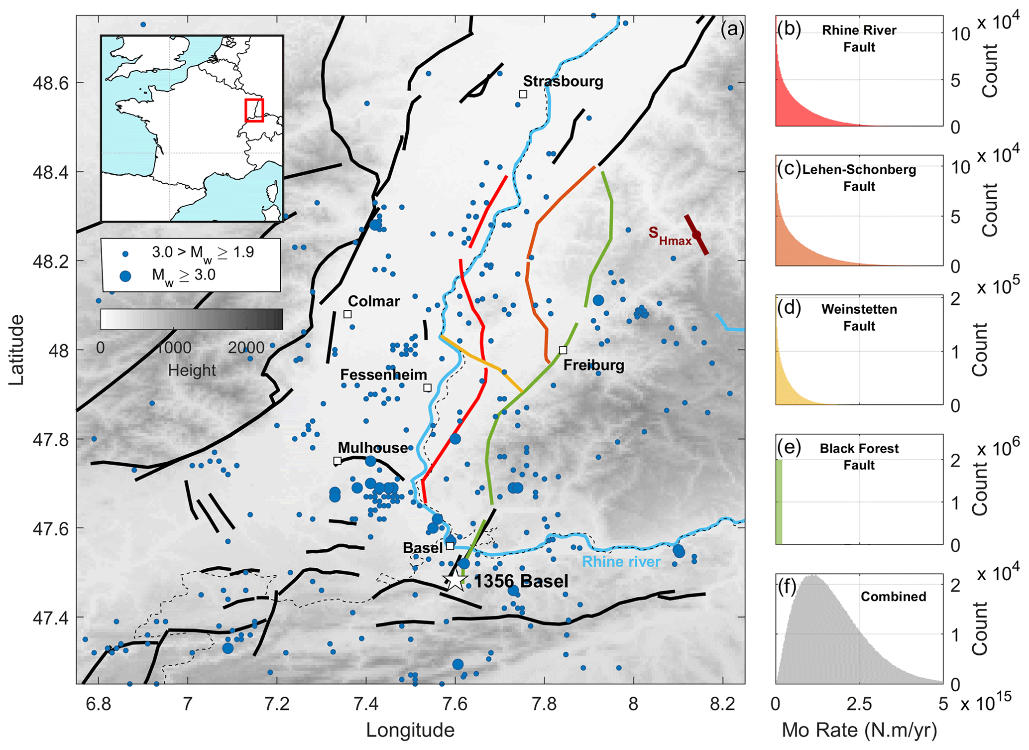
Figure 1(a) Regional setting and seismicity of the Upper Rhine Graben (Drouet et al., 2020). Black lines are faults, while colored ones are the faults taken into account in this study. The fault network geometry is based on the BDFA database (Jomard et al., 2017) and Nivière et al. (2008). Blue dots are epicenters of Mw>2.2 earthquakes since 1994. The white star indicates the 1356 Basel earthquake (magnitude ranging from M6.5±0.5, Manchuel et al., 2018, to M6.9±0.2, Fäh et al., 2009). The brown bar indicates the approximate orientation of the maximum horizontal compressional stress () (Heidbach et al., 2016, 2018). The thin dashed black line is the border between France and Germany. The nuclear power plant of Fessenheim and the main cities are indicated by white squares. (b–f) Moment deficit rate probability density functions (PDFs); expressed in counts for each of the four faults considered (colors are indicative of the faults in the left panel) and their combination (in gray).
The seismic hazard of the URG has been evaluated by multiple studies at the national/European scale (Grünthal et al., 2018; Drouet et al., 2020; Danciu et al., 2021). Furthermore, the seismic hazard of the southern region of the URG in particular has recently been assessed by Chartier et al. (2017) with a focus on the Fessenheim nuclear power plant (Fig. 1). This study evaluates the seismic hazard using a fault-based approach, taking into account the network of potentially active faults characterized by Jomard et al. (2017). This fault-based work involves a moment budget approach, which involves comparing the rate of moment release by seismicity and the rate of moment deficit (MDR) accumulating along locked portions of faults between large earthquakes (i.e., the tectonic loading rate of each fault). Since the period of seismological observation (a few centuries) is too short to be representative of the long-term behavior of seismicity, Chartier et al. (2017) instead built a seismicity model assumed to be representative of the long-term magnitude–frequency distribution (MFD) of earthquakes, a method similarly used in former studies (e.g., Molnar, 1979; Anderson and Luco, 1983; Avouac, 2015). Earthquakes below Mw 5 are disregarded (Bommer and Crowley, 2017; Chartier et al., 2017). Earthquakes between Mw 5 and 6 are assumed to follow the MFD of the catalog of earthquakes they consider. This catalog integrates several sources of instrumental and historical earthquakes including sources from the Laboratoire de Détection et de Géophysique of the Commissariat à l'Énergie Atomique et aux énergies alternatives (CEA-LDG; http://www-dase.cea.fr/, last access: 19 January 2024) and from the FPEC (French Parametric Earthquake Catalogue; Baumont and Scotti, 2011), the Institut de Radioprotection et de Sûreté Nucléaire (IRSN) contribution to SHEEC (SHARE European Earthquake Catalogue; Stucchi et al., 2013). MFDs are estimated based on a French seismotectonic zoning scheme defined by Baize et al. (2013). Earthquakes with magnitudes above Mw 6 are assumed to occur on the fault planes (Jomard et al., 2017). Chartier et al. (2017) consider two types of model: (1) each fault ruptures only as its maximum-magnitude event, which is controlled by the surface area of the seismogenic fault segment (characteristic earthquake model); (2) events follow the Gutenberg–Richter (GR) law with a b value equal to 1, and the maximum magnitude, Mmax, is fixed as in the previous model. The recurrence times of the Mw>6 events are then calibrated so that the rate of moment released by the seismicity models matches the MDR estimated from neotectonic data (Chartier et al., 2017; Jomard et al., 2017). The authors explore different fault geometries (e.g., dip and seismogenic depth) using a logic-tree methodology and then proceed to the probabilistic seismic hazard assessment (PSHA) of the region, providing a map of the probability of exceedance of peak ground acceleration (PGA) within a time period.
A number of strong assumptions are made within this framework. As mentioned previously, a simplified fault network is used (Jomard et al., 2017), which constrains the seismogenic area available for ruptures. Expert choices have also been made to distribute slip rates (i.e., loading rates) originally attributed to faults that have been removed from the initial fault network (Nivière et al., 2008) on other fault segments. On a number of faults, no estimates of neotectonic slip rate are available (e.g., West Rhenish Fault) and the authors have chosen to apply slip rates equivalent to those from other nearby faults (0.01 to 0.05 mm yr−1). The neotectonic data are actually only along-dip slip rate estimates. No along-strike slip rates have yet been published due to the lack of markers to quantify horizontal offsets along faults, and this component has thus been ignored. In addition, Chartier et al. (2017) do not consider continuous probabilities as they apply a logic-tree method. Chartier et al. (2017) fix the b value to 1, choose the seismogenic depth to be either 15 or 20 km, and do not take into account multi-segment ruptures when estimating Mmax for each fault segment.
In this study, we build upon Chartier et al. (2017) seismic hazard evaluation of the southern URG by exploring uncertainties in greater detail, revisiting a number of assumptions. We use the methodology from Rollins and Avouac (2019) and Michel et al. (2021), which allows us to evaluate the seismogenic potential of faults in a probabilistic fashion and explore uncertainties for parameters such as the b value or Mmax. We use the fault network and slip rates taken into account by Nivière et al. (2008), disregarding the West Rhenish Fault, for which, to our knowledge, no slip rate data are available. We assume faults can rupture simultaneously (i.e., multi-segment rupture). In the following sections, we start by describing the concepts and methods we use to constrain the seismogenic potential of the URG, and then we describe the data available before discussing the robustness of our results.
We use the methodology from Michel et al. (2021) in order to estimate the seismogenic potential of the upper Rhine Graben, including Mmax and its recurrence time. As in Chartier et al. (2017), we produce seismicity models representative of the long-term behavior of earthquakes. We assume that the MFDs of background earthquakes follow a Gutenberg–Richter power law up to Mmax. We define background earthquakes as mainshocks, as opposed to their subsequent aftershocks. We assume that their timing of occurrence is random, following a Poisson process. Each model is controlled by three parameters: (1) Mmax; (2) the recurrence time of events of a certain magnitude, τc; and (3) the b value. We use two types of model, namely the tapered and truncated models (Rollins and Avouac, 2019; Michel et al., 2021; Fig. S1 in the Supplement). The tapered model type assumes a non-cumulative power-law MFD truncated at Mmax, which gives rise to a tapered MFD in the cumulative form (i.e., the traditional display when representing the Gutenberg–Richter law). The truncated model type assumes instead a MFD with a distribution truncated at Mmax in the cumulative form.
The seismicity models are then tested against three constraints: (1) the moment budget, as in Chartier et al. (2017), which implies that the moment released by slip on the fault should match the moment deficit accumulating between earthquakes over a long period of time; (2) the moment–area scaling law, an empirical scaling law relating rupture area to slip for each earthquake; and (3) the MFD of observed seismicity. Each of these constraints is described in more detail in the following sub-sections. The data and associated uncertainties used for the constraints are discussed in the following section (i.e., Sect. 3).
2.1 Moment budget
A moment budget consists in comparing the rate of moment released from slip events (seismic or aseismic), , with the moment deficit rate, , accumulating between slip events. The moment deficit rate is defined by the equation , where μ is the shear modulus, A is the area that remains locked during the interseismic period (i.e., the potential seismogenic zone) and is the rate at which slip deficit builds up. Since the distribution of locked segments of faults and their associated loading rates cannot yet be determined for the URG from geodetic measurements, A is assumed to be homogeneous along-strike for each fault, while we consider it possible for the seismogenic width to change from one fault to another. The rate at which slip deficit builds up, , is evaluated based on neotectonic information (see Sect. 3.1). The total moment released, , is calculated based on the rate of moment release of the long-term seismicity model. Since the long-term seismicity model only considers mainshocks, we included a fourth parameter, αs, that represents the proportion of moment released by background seismicity (Avouac, 2015), , relative to the total moment released (including aftershocks and aseismic afterslip). If , then the moment budget is said to be balanced.
The cumulative MFDs for tapered and truncated seismicity models achieving a balanced moment budget have an analytical form and are a function of Mmax, b, and αs (see Rollins and Avouac, 2019, and references therein). We can therefore estimate the probability of a seismicity model balancing the moment budget, PBudget, by sampling the a priori distributions of those parameters.
2.2 Moment–area scaling law
According to global earthquake statistics, the moment released by an earthquake, , is proportional to the area of its rupture, Aeq, such that (Wells and Coppersmith, 1994; Leonard, 2010; Stirling et al., 2013). We use this scaling to evaluate whether a seismic event of a given magnitude has a rupture area that fits within the seismogenic zone. By considering the spread of the empirical distribution of magnitude vs. area, we assume the probability distribution function of an event of magnitude Mw to be probable considering this scaling, PScaling. We use here the self-consistent scaling law, and related uncertainties, as defined by Leonard (2010) in the dip-slip equation (the strike-slip equation is in any case almost the same).
2.3 Earthquake catalog
We test whether the observed MFD from earthquake catalogs may be a sample of the distribution of the long-term seismicity models we are building. Effectively, we evaluate the likelihood of our observed MFD given the distribution of the models. Since we only consider mainshocks, we define the likelihood of the observed seismicity catalog, PCat, as , where is the probability of observing events within the magnitude bin Mi that occur during the time period , assuming the long-term mean recurrence of events is :
Effectively, for a given seismicity model, we randomly generate 2500 declustered earthquake catalogs. We evaluate the likelihood of each catalog and define PCat as the average of these likelihood values.
Note that we follow the recommendation by Felzer (2008) while exploring magnitude uncertainties and correct the magnitudes of each event by , where b is the declustered catalog b value, σ is the standard deviation for the event's magnitude and e is the exponential constant.
2.4 Seismicity model probability and marginal probabilities
Finally, the probability of a seismicity model is defined as PSM=PBudgetPCatPScaling, which depends, among others, on Mmax and b (Michel et al., 2021). The evaluation of the parameters to estimate PSM is discussed in Sect. 3. Marginal probabilities such as , the probability of Mmax, and Pb, the probability of the b value, can be estimated based on PSM. We also define P(τmax|Mmax) as the probability of the rate of Mmax, and P(τ|Mw) as the probability of the rate of events with magnitude Mw, which accounts for all earthquakes from all of the models (i.e., not only Mmax). Probabilities needed for estimating seismic hazard (e.g., PSHA) such as the probability of having an event above magnitude Mw for a time period T, P(M>Mw|T), can likewise be evaluated.
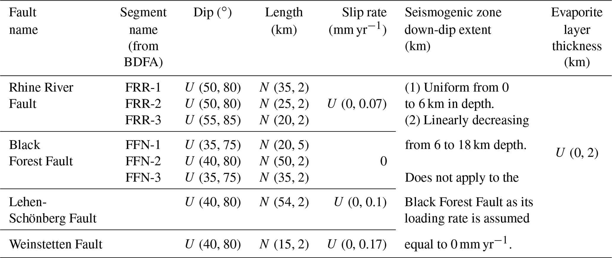
We present in this section the data and their associated uncertainties used to evaluate each constraint. Hereafter, the U and N symbols will stand for uniform and normal distribution, respectively. Table 1 summarizes the uncertainties taken for each parameter.
Table 1Fault parameters. U and N stand for uniform and normal distribution. The PDFs of each of these parameters and the resulting moment deficit rate for each fault are shown in Figs. S3–S6.
3.1 Neotectonic data, seismogenic along-dip width and moment deficit rate
In order to evaluate the MDR for the moment budget constraint (Sect. 2.1), we must infer estimates of the loading rate (i.e., ) for each fault taken into account. The slip rate on each fault is taken from Nivière et al. (2008) for the Rhine River, Black Forest, Weinstetten and Lehen-Schönberg faults (the Landeck and West Renish faults are not considered). Their slip rates rely on estimates of the cumulative vertical displacement of the faults based on Pliocene–Quaternary sediments thickness variations measured from 451 boreholes, assuming that the accommodation space opened by tectonic motion is completely balanced (or over-balanced) by sedimentation. However, potential erosional periods due to the piracy of the Rhine River might bias the measurements; thus the values are to be interpreted as maximum displacement estimates. Nivière et al. (2008) inferred vertical slip rates of 0.07 and 0.17 mm yr−1 from the age of the sediments for the Rhine River and Weinstetten faults, respectively. The Lehen-Schönberg Fault slip rate reaches between 0.04 and 0.1 mm yr−1. While borehole observations do not allow us to conclude on the Pliocene–Quaternary slip rate of the Black Forest Fault, this structure is suggested to be inactive during this time period, and the deformation is now accommodated by the other aforementioned faults (Nivière et al., 2008). Note that these are vertical slip rate estimates and the along-strike component is for the moment neglected. For the moment rate calculation, we project vertical slip rates on the along-dip direction considering the dip angles of each fault.
The seismogenic down-dip extent of a fault depends on the temperature gradient (e.g., Oleskevich et al., 1999), among other parameters. Indeed, between the isotherms 350 and 450 ∘C, quartzo-feldspathic rocks undergo a transition in frictional properties (Blanpied et al., 1995) from a rate-weakening (<350 ∘C), potentially seismogenic behavior to a rate-strengthening (>450 ∘C), stable sliding behavior (Dieterich, 1979; Ruina, 1983). The geothermal gradient below the URG is higher than in the surrounding regions due to its tectonic history (Freymark et al., 2017). Based on borehole temperature measurements from Guillou-Frottier et al. (2013), we estimate the envelopes of the geothermal gradient in the southern URG (Fig. S2), assuming a linear temperature gradient with depth, and show that the frictional property transition would occur between depths of 6 km (shallowest position of the 350 ∘C isotherm; Fig. S2) and 18 km (deepest position of the 450 ∘C isotherm; Fig. S2). In this study, we define the PDF of the seismogenic down-dip extent as a uniform distribution between 0 and 6 km depth associated with a linear taper down to 18 km. The linearity of the taper implies that the position of the fault's transition to a fully rate-strengthening behavior (>350–450 ∘C) has a uniform probability of falling between 6 km (shallowest position of the 350 ∘C isotherm according to Fig. S2) and 18 km depth (deepest position of the 450 ∘C isotherm; Fig. S2), i.e., rate − strengthening transition ∈ U(6, 18) km.
Additionally, the southern part of the URG is the site of a potash-salt evaporitic basin (Lutz and Cleintuar, 1999; Hinsken et al., 2007; Freymark et al., 2017), which reaches a maximum depth of ∼2 km. Such formations may not accumulate any moment deficit as the yield stress of evaporites is very low (Carter and Hansen, 1983). We assume that each fault is potentially impacted by this formation, hence modulating the seismogenic thickness and in turn the seismogenic area available for a rupture. The resulting PDF for the seismogenic thickness is the convolution of the PDF of the down-dip extent of the seismogenic zone with the PDF of the evaporitic basin thickness taken as U(0, 2) km. Combining both temperature and salt basin assumptions leads to a PDF of the along-dip seismogenic width, which is uniform down to ∼5 km and decreases linearly until ∼17 km (Figs. S3–S6).
The moment deficit is then the product of the length of each fault, their seismogenic width, the neotectonic long-term slip rate and the shear modulus that we fix to 30 GPa (same as in Chartier et al., 2017). Each fault is assumed to have its own seismogenic width. The moment deficit rate of each fault is shown in Fig. 1. The PDFs for each of the fault's constitutive parameters are shown in Figs. S3–S6. By considering the range of the fault's geometrical parameters, which also considers the Black Forest Fault even though it is assumed to be non-active, we obtain the moment–area constraint shown in Fig. 2. Events of up to Mw 6.5 are equiprobable, while those above Mw 7.7 are extremely improbable.
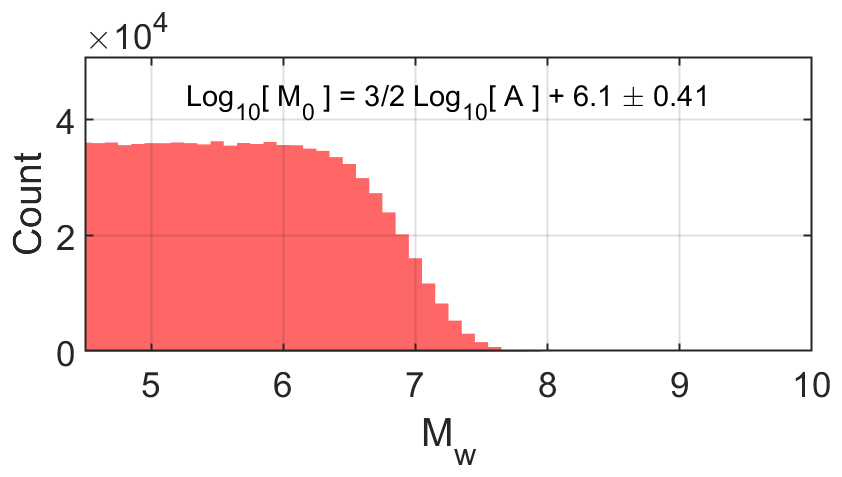
Figure 2PDF of Mw considering the along-dip moment–area scaling law of earthquakes from Leonard (2010). Note that the area from the Black Forest Fault is not included, as its loading rate is assumed equal to 0 mm yr−1.
3.2 Instrumental and historical seismicity catalogs
To constrain the MFD of the long-term seismicity models with an observational seismicity catalog, as described in Sect. 2.3, we need to evaluate from the observational catalog the number of events per magnitude bin over a period of time (Sect. 2.3). We use the earthquake catalog from Drouet et al. (2020). This catalog was built from multiple former catalogs. It relies mostly on the FCAT-17 catalog (Manchuel et al., 2018), which is itself a combination of the instrumental catalog SiHex (SIsmicité de l'HEXagone; Cara et al., 2015) for the 1965–2009 period and a historical catalog based on the macroseismic database of SisFrance (BRGM, IRSN, EDF), intensity prediction equations from Baumont et al. (2018) and the macroseismic moment magnitude determination from Traversa et al. (2018) for the 463–1965 period. Events located more than 20 km from the French border, not provided by FCAT-17, are based on the SHEEC catalog (Stucchi et al., 2013; Woessner et al., 2015). Finally, events between 2010 and 2016 come from the CEA-LDG bulletins (https://www-dase.cea.fr, last access: 19 January 2024). All event magnitudes are given in Mw, and uncertainties are provided. Anthropic events are expected to have already been removed from the catalog (Cara et al., 2015; Manchuel et al., 2018).
We select events within the coordinates [47, 49.5∘] latitude and [6, 8.5∘] longitude, i.e., a broad region covering the whole URG, and divide the catalog into two time periods, an instrumental period and a historical one taking events from 1980 onwards and 1850 onwards, respectively. We decluster both catalogs to compare them with the long-term seismicity models (Sect. 2.3). Declustering is based on the methodology of Marsan et al. (2017), which evaluates the probability that an earthquake is a mainshock. Declustering is applied based on a completeness magnitude, Mc, of 2.2 and 3.2 for the instrumental and historical catalogs, respectively (Sect. S1 in the Supplement; Figs. S7 and S8). From the resulting catalogs, we keep events from 1994 onwards and 1860 onwards for the instrumental and historical catalogs, respectively (Figs. S7 and S8), in order to avoid border effects from declustering. For the instrumental catalog, 1994 is also the date from which the seismicity rate appears relatively constant (Fig. S7). We then select events in the region of interest (i.e., the southern part of the URG), taking into account only earthquakes located within a 10 km buffer around the faults considered, including the Black Forest Fault (Fig. 3). Note that since no events below Mc are considered, there is a lack of events which fall in the magnitude bins directly above Mc while exploring magnitude uncertainties. Thus, when applying the earthquake catalog constraint (Sect. 2.3), we take events with Mw≥2.8 and Mw≥4.3 for the instrumental and historical catalogs, respectively (Felzer, 2008) (Fig. 3).
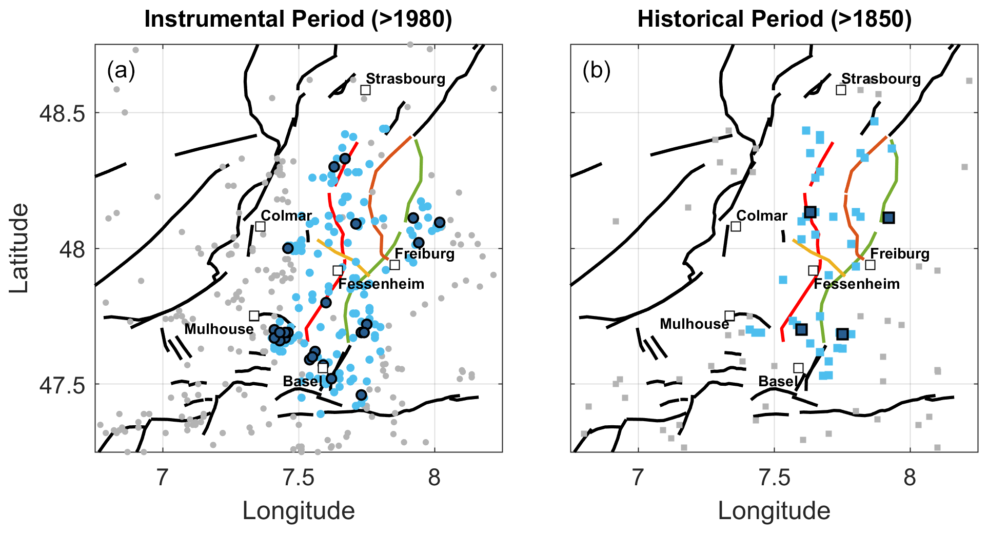
Figure 3Earthquake selection for the (a) instrumental (>1994) and (b) historical (>1850) periods. Gray dots and squares indicate all earthquakes with Mc=2.2 and 3.2 for the instrumental and historical catalogs, respectively. Light-blue dots and squares indicate earthquakes taken into account for the seismogenic potential analysis. Dark-blue dots and squares indicate Mw≥2.8 and 4.3 earthquakes taken into account for the seismogenic potential analysis.
3.3 Constitutive parameters of seismicity models
As mentioned in Sect. 2.1, the cumulative MFD for tapered and truncated seismicity models balancing the moment budget can be defined as a function of Mmax, b, and αs. We explore these parameters using a grid search with Mmax and b sampled uniformly over and , respectively. Based on global statistics of the post-seismic response following earthquakes (Alwahedi and Hawthorne, 2019; Churchill et al., 2022), we assume that the PDF of αs is a Gaussian distribution with N(0.9, 0.25) (Fig. S9). Finally, the PDF of the MDR for each fault is assumed to be uniform between 0 and the estimate based on the maximum slip rate from Nivière et al. (2008) (Sect. 3.1). We thus include scenarios for which almost no moment deficit accumulates on the fault (i.e., the fault slips aseismically or accumulates no strain over long periods of time). This assumption contrasts with the choice made by Chartier et al. (2017), who assume that each fault is fully locked over a seismogenic width terminating at either 15 or 20 km. In doing so, we explore a broad range of possible models.
The combination of constraints (Sect. 2) leads to the results shown in Fig. 4. For the truncated model, the marginal probability of PSM in the Mmax and τmax space is represented by the gray-shaded distribution in Fig. 4 (not shown for the tapered model since the models taper at Mmax). The marginal probability of Mmax for the tapered model (in green) peaks at 6.1, while the one for the truncated model (in blue) is bi-modal with peaks at 5.2 and 5.8. For the truncated model (not the tapered model for the same reason as previously indicated), the marginal probability P(τmax|Mmax=5.8) (solid blue line on the y axis) peaks at ∼1000 years. Taking Mmax=6.6 or 7.0, a number close to the estimated magnitude of the 1356 Basel earthquake, the marginal probability would instead peak at ∼16 000 and ∼80 000 years, respectively.
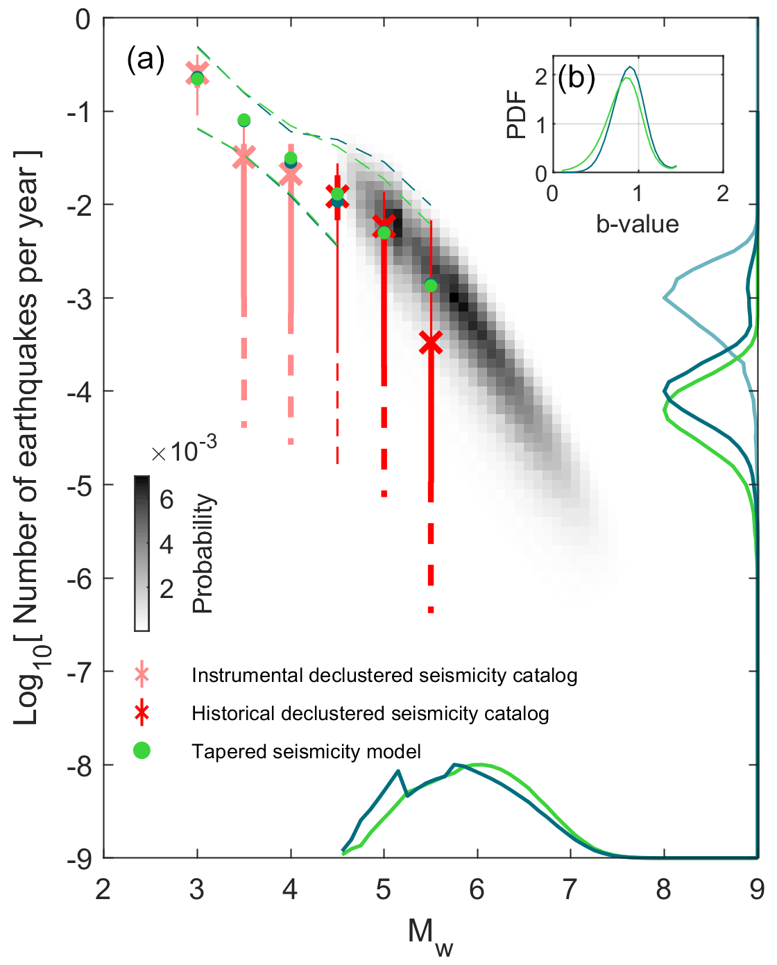
Figure 4(a) Seismogenic potential of the URG using all constraints: moment budget, observed magnitude–frequency distribution and moment–area scaling law. The rates of occurrence of historical and instrumental earthquakes, within their observation periods, are indicated by red and pink crosses and error bars, respectively. Thick and thin error bars indicate the 15.9 %–84.1 % (1σ) and 2.3 %–97.7 % (2σ) quantiles of the MFDs. Dashed lines show the spread of possible MFDs for the 2500 catalogs randomly generated to explore uncertainties. The green and blue colors are associated with the tapered and truncated long-term seismicity models. Green and blue dots show the means of the marginal PDF for the long-term seismicity. Dashed green and blue lines indicate the spread of the best 1 % of seismicity models. The marginal probabilities of Mmax, , are indicated by the solid lines on the Mw axis. They have been normalized so that their amplitude is equal to one instead of 0.60 and 0.59 for the tapered and truncated models, respectively. Green and dark-blue lines on the earthquake frequency axis indicate the probability of the rate of events, τ, with magnitude Mw=MMode, thus P(τ|Mw=MMode), with MMode=6.1 and 5.8 for the tapered and truncated models, respectively, considering all magnitudes in the seismicity models and not only the recurrence rate of Mmax. They have also been normalized, and their peaks were initially at 1.13 and 1.17 for the tapered and truncated models, respectively. The light-blue line on the earthquake frequency axis indicates P(τmax|Mmax=5.8) (for the truncated seismicity model only) and is normalized so that its amplitude equals 1 instead of 1.19. Note that the seismicity MFDs shown in the figure are not in the cumulative form. (b) Marginal probability of the b value.
The marginal probabilities P(τ|Mw=6.1) and P(τ|Mw=5.8) for the tapered and truncated models (dotted green and blue lines, respectively, on the y axis), which take all events from the seismicity models into account (not only Mmax), have instead peaks at ∼16 000 and ∼10 000 years, respectively. The marginal probability Pb peaks at ∼0.85 and 0.9 for the tapered and truncated models, respectively.
The effect with and without the moment–area scaling law is shown in Fig. 5. Adding the scaling law constraint does not change the mode of but completely rejects scenarios with Mmax>7.8.
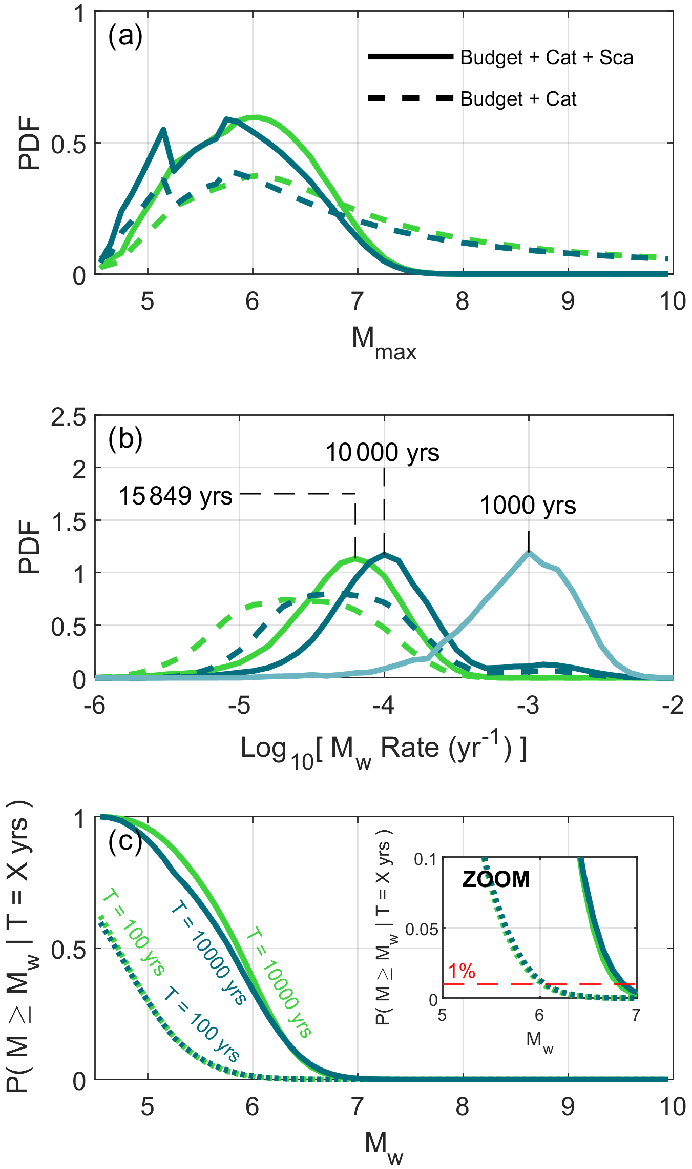
Figure 5(a) Evolution of the marginal PDF of Mmax when adding the moment–area scaling law constraint. The green and blue colors in the figure are associated with the tapered and truncated long-term seismicity models. (b) The same as (a) but for the marginal PDF of the recurrence time of events: P(τ|Mw=6.1) and P(τ|Mw=5.8) for the tapered and truncated models (dark-blue and green lines), respectively, and P(τmax|Mmax=5.8) shown only for the truncated model (solid light-blue line). (c) Probability of occurrence of earthquakes with a magnitude larger than Mw over a period of X years. We show the probability of occurrence of such events for the 100- and 10 000-year time periods. In (a)–(c), dotted lines represent the marginal PDFs considering both the moment budget and the seismicity catalog constraint and dashed lines indicate the PDFs when the earthquake scaling constraint is added. The inset in (c) is a zoomed-in part of the panel. The 1 % probability of exceedance over a time period of 100 years is a typical order of magnitude for nuclear applications in France.
Finally, the probabilities P(M>Mw|T) for T=100 and 10 000 years are also shown in Fig. 5. As an example, the probability of occurrence for an event above Mw 6.5 (similar to the 1356 Basel earthquake) for an observational period of 100 years is ∼0.1 % for both the tapered and the truncated models. For an event above Mw 6.0 and for the same period, this probability is instead ∼1 % for both models (see zoomed-in inset in Fig. 5c).
The correlations between Mmax, the moment deficit rate, the b value and αs, for both the tapered and the truncated models but without the scaling law constraint, are shown in Figs. S10 and S11. For both models, probable Mmax increases with an increasing b value (Figs. S10a and S11a), highlighting strong interdependency between the two parameters. Raising the moment deficit rate will control the minimum probable Mmax (Figs. S10b and S11b) but will also tend to exclude scenarios with a high b value (>1.25; Figs. S10f and S11f). While other trends are expected between parameters, they seem less visible likely due to the uncertainties in the parameters explored, and we thus do not pursue further analysis between those parameters.
The results if we combine the PDFs from the tapered and truncated models using a mixture distribution are shown in Fig. S12. has a main peak at 5.9 and a smaller peak at 5.2, which originates from the truncated model. P(τ|Mw=5.9) peaks instead at ∼13 000 years.
5.1 Sensibility to earthquake catalog declustering
The catalog declustering (i.e., removal of aftershocks) may have a significant impact on the results (Sect. 2.3), influencing the shape of the observed MFD of earthquakes. In this study, we applied the methodology of Marsan et al. (2017), which is based on the epidemic-type aftershock sequence (ETAS) framework and intrinsically assumes that background events have Poisson behavior. Other declustering methodologies are available, and here we test the one from Zaliapin and Ben-Zion (2013) based on the nearest-neighbor distances of events in the space–time–energy domain. The results from this methodology produce background seismicity catalogs with more events than the one from Marsan et al. (2017) (Sect. S2 and Figs. S13–S15) but imply larger b values when combining the instrumental catalog with the historical one (as inferred by Fig. 6b). The analysis of the seismogenic potential of the URG using the Zaliapin and Ben-Zion (2013) methodology results in peaking at M6.3 for the tapered model and is still bi-modal for the truncated model, with peaks at M5.2 and M5.9 (Fig. 6). Unlike with Marsan et al. (2017), the peak at lower magnitude for the truncated model is more probable than the one at larger magnitude. The most probable Mmax for both models are slightly shifted to lower magnitudes than the values estimated using the Marsan et al. (2017) methodology, but the width of the PDFs appears unchanged to first order. The resulting marginal probabilities P(τ|Mw=5.9) and P(τ|Mw=5.8) for the tapered and truncated models both peak at ∼8000 years.
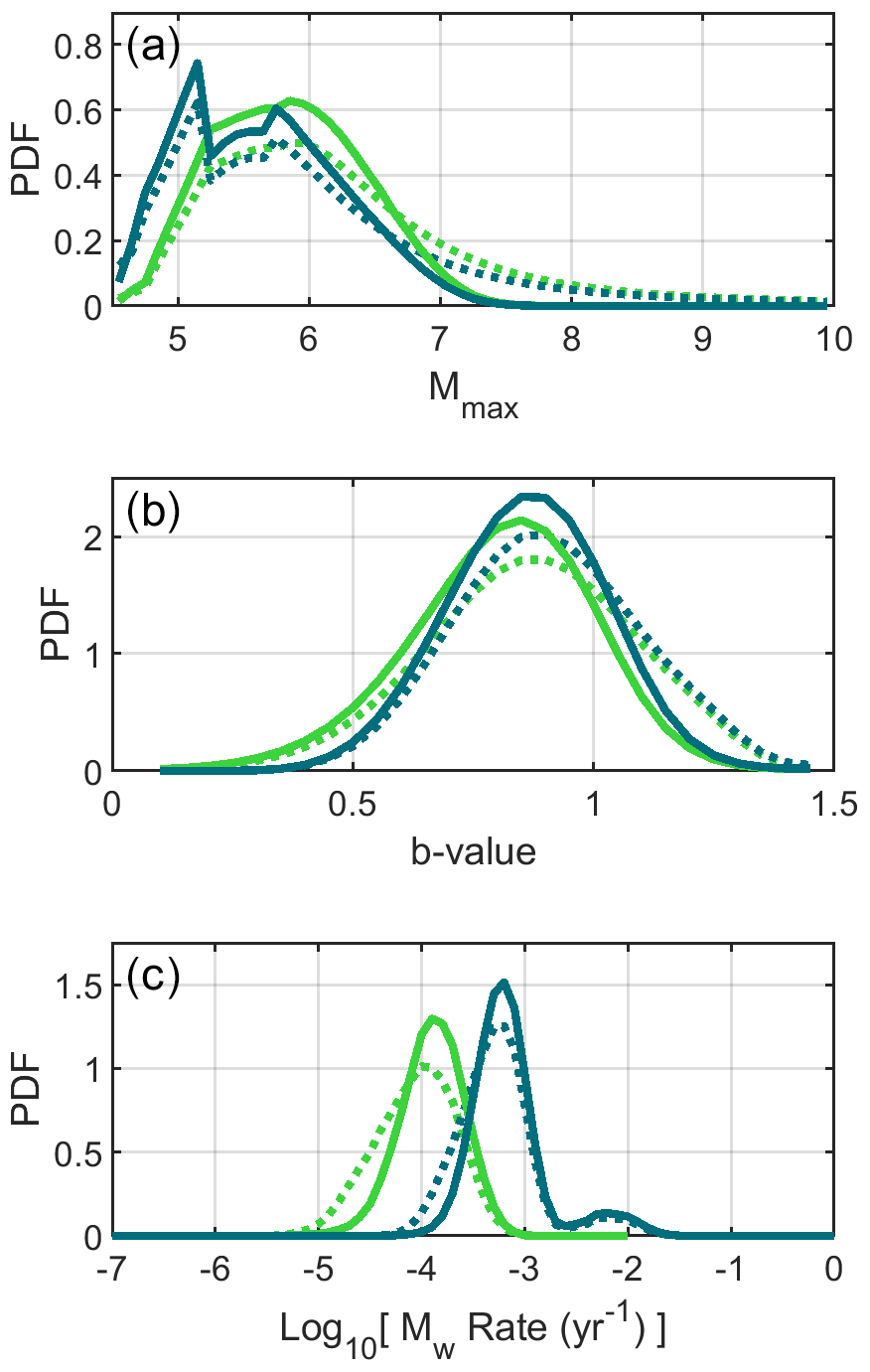
Figure 6Results using the declustering method from Zaliapin and Ben-Zion (2013) instead of Marsan et al. (2017) (Sect. S2). In this scenario, no probabilities of events being mainshocks are defined. (a) The Mmax PDF. (b) The b-value PDF. (c) The P(τ|Mw=MMode) PDF. Solid lines correspond to the results using all constraints, while the dotted lines only use the moment budget and earthquake catalog constraints. Green and blue lines correspond to the tapered and truncated models, respectively. The results shown here are the ones taking a b value equal to 1 for the Zaliapin and Ben-Zion (2013) declustering method. The results for b values of 0.5 and 1.5 are also shown in Fig. S15 and are relatively similar to the ones obtained using a b value of 1.0.
5.2 Source of seismicity
We initially selected earthquakes within a 10 km buffer zone around the faults to reflect the spatial strain pattern of a vertical fault blocked down to a depth of 10 km. Nevertheless, the locking depth could potentially be deeper, down to ∼18 km as suggested in Sect. 3.1. In this respect, we also provide results if events are selected within 20 km of the faults (Figs. S16 and S17). Under these conditions, the seismicity rates of the observational earthquake catalogs are higher and constrain the long-term seismicity models to cases that produce a higher moment release rate. thus favors events with a lower magnitude than the one using events within 10 km (Fig. 5; Sect. 4). The tapered model peaks at Mw 5.9, instead of 6.1, while the truncated model peaks twice at Mw 5.2 and 5.8, in a similar manner to the reference scenario in Sect. 4, except that the peak at Mw 5.2 is now the most probable.
However, current seismicity in the URG is seemingly diffuse and it is difficult to associate it with a fault in particular (Doubre et al., 2022). On the other hand, geodetic data are not yet able to resolve any tectonic deformation and thus to evaluate the loading rate of faults (Henrion et al., 2020). Even though the Drouet et al. (2020) catalog, based on the FCAT-17 catalog, is supposedly devoid of anthropic seismicity (Cara et al., 2015; Manchuel et al., 2018), one can then ask whether the current seismicity is totally representative of the undergoing long-term tectonic processes or presently modulated by surface loads such as the post-glacial rebound (e.g., Craig et al., 2016), aquifer loads, erosion or incision (e.g., Bettinelli et al., 2008; Steer et al., 2014; Craig et al., 2017). If so, the assumption that the main driver of seismicity is tectonic loading breaks down and our method used to assess seismic hazard must be completed by physics-based constraints of such transient stress release (Calais et al., 2016). Distinguishing seismic sources triggered by tectonic loading from other driven forces is an extremely difficult task. The earthquake catalog contribution (Sect. 2.3) might then not be appropriate.
Additionally, the magnitudes of historical events from the FCAT-17 catalog (before the 1960s), and thus the ones from Drouet et al. (2020), seem to be overestimated (or the instrumental events have underestimated magnitudes even though this seems less probable), and a bias in the MFD is thus expected (Beauval and Bard, 2022; Doubre et al., 2022). For the URG case, three bins out of seven of the observed MFD are estimated from the instrumental period. The bins estimated from the historical period have thus slightly more weight in the catalog constraint (Sect. 2.3).
We test an alternative constraint inferring that the possible magnitude and frequency of Mmax must be consistent with the largest observed event over the observation period (∼146 years), meaning that it has to be larger than or equal to the largest known event while the return period of the largest event cannot be significantly shorter than the observation period (Approach 2 from Michel et al., 2018). This constraint is equivalent to considering that no earthquakes with a magnitude greater than the largest event in the observation period occurred during the time period covered by the observed catalog. Theoretically, this constraint imposes a lower bound on Mmax and its recurrence time. The results obtained using this constraint together with the moment budget and scaling law ones are shown in Fig. 7. Since Mmax frequency differs for the tapered and truncated models, the new constraint imposes different lower bounds for the two models. The truncated model rejects scenarios with Mmax below Mw 5.5 more strongly. Pb is not constrained by the observed seismicity catalog, but higher values of the b value seem slightly more probable (inset in Fig. 7). The marginal probabilities P(τ|Mw=5.9) and P(τ|Mw=6.3) for the tapered and truncated models have peaks at ∼12 500 and ∼63 000 years, respectively.
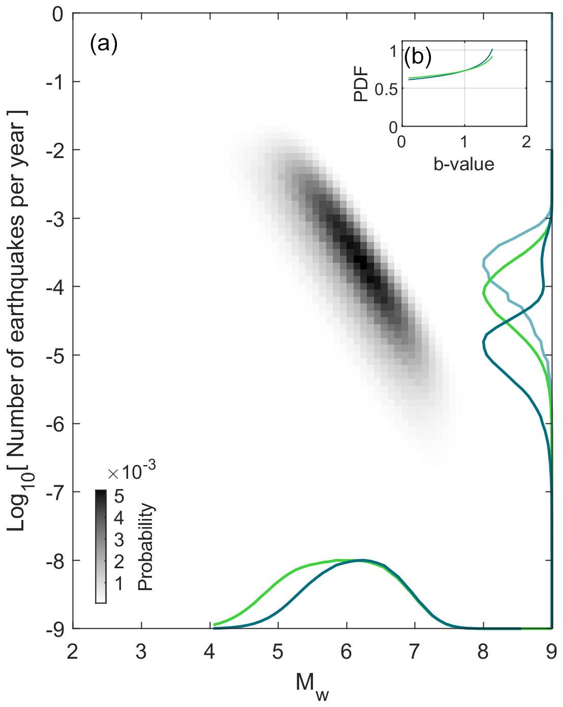
Figure 7Same as Fig. 4 but only considering the constraints for the moment budget, for the moment–area scaling law and on Mmax frequency considering the time period of the catalog (which serves as a lower-bound constraint for Mmax; Sect. 5.2; Approach 2 from Michel et al., 2018). The marginal probabilities have been normalized so that their amplitude is equal to 1 instead of 0.46 and 0.58 for the tapered and truncated models, respectively. The same is true for P(τ|Mw=MMode), which was initially with 0.85 and 0.81 amplitude, and P(τmax|Mmax=6.3) (for the truncated seismicity model only), which peaked at an amplitude of 0.85.
5.3 Strike-slip component
In this study, as well as in Chartier et al. (2017), we assume solely along-dip displacement since it is the only published neotectonic information available. Nevertheless, recent paleoseismological data on the Black Forest Fault near Karlsruhe (north of our study area) suggest 5.9 m of cumulative strike-slip faulting, in contrast to 1.2 m of cumulative vertical slip, over the last 5.9 kyr (Pena-Castellnou et al., 2023). Those displacements seem to be associated with at least three paleo-earthquakes. This suggests (1) that the Black Forest Fault has been active during the Quaternary period and (2) that strike-slip faulting might be predominant. The ratio between strike- and dip-slip faulting from the Black Forest event would be then equal to 4.8. We thus test a scenario where the Black Forest Fault is associated with a maximum vertical slip deficit rate of 0.18 mm yr−1, as proposed by Jomard et al. (2017), where we multiply the maximum slip deficit rate of all faults considered by 4.8. The results and the revised MDR for each fault are shown in Figs. 8 and S18. peaks at Mw 6.8 and Mw 6.6 for the tapered and truncated models, respectively. They are associated with the marginal probabilities P(τ|Mw=6.8) and P(τ|Mw=6.6) that both peak at ∼16 000 years for the tapered and truncated models. Note that Pena-Castellnou et al. (2023) suggest that earthquakes of potentially Mw 6.5 occurred north of our study area. Pb peaks at 0.7 for both the tapered and the truncated models, thus at lower values than taking into account the vertical slip component alone.
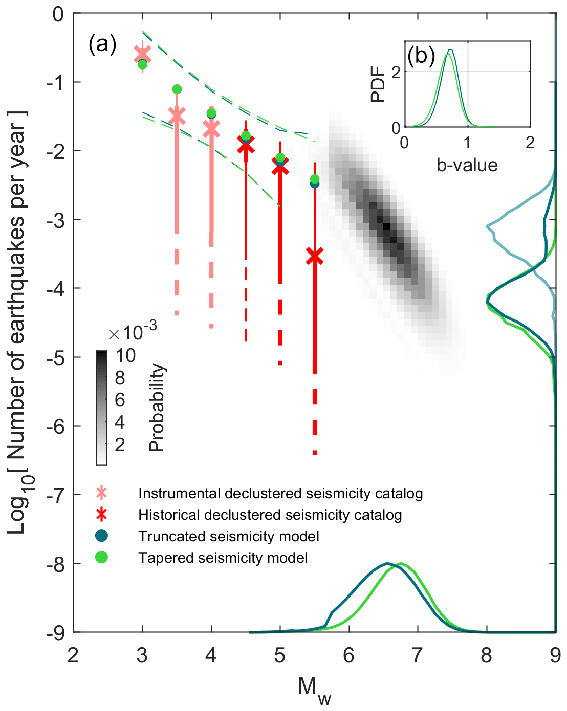
Figure 8Same as Fig. 2 but considering a strike-slip slip rate component equivalent to 4.8 times the dip-slip estimate and assuming the Black Forest Fault maximum long-term vertical slip rate is 0.18 mm yr−1 (as proposed by Jomard et al., 2017). The Leonard et al. (2010) strike-slip moment–area scaling law is used here for the scaling law constraint, even though it is very similar to the dip-slip version. The marginal probabilities have been normalized so that their amplitude is equal to 1 instead of 1.02 and 0.88 for the tapered and truncated models, respectively. The same is true for P(τ|Mw=MMode), which was initially 1.15 and 1.13 in amplitude, and P(τmax|Mmax=6.6) (for the truncated seismicity model only), which peaked at an amplitude of 1.17.
The previous scenario tested (Fig. 8) takes two more faults (i.e., Weinstetten and Lehen-Schönberg faults) into account than in Chartier et al. (2017), as these two faults are not present within the BDFA (the French database of potentially active faults; Jomard et al., 2017). The results obtained by selecting faults as defined by Chartier et al. (2017) and applying the strike-slip assumption are provided in Fig. S19. peaks at Mw 6.7 and Mw 6.6 for the tapered and truncated models, respectively, which is very similar to the scenario taking all four faults, as the moment deficit rate is dominated by the Rhine River and Black Forest faults. Note that the marginal probabilities P(τ|Mw) and P(τmax|Mmax) seem to get more noisy, likely due to the shape of the MDR PDF, which skews heavily towards zero (black line in Fig. S18e).
5.4 Multi-segment rupture
In this study we assume that all faults can rupture simultaneously. Nevertheless, the Black Forest Fault is initially taken as inactive, and the traces of the Weinstetten and Lehen-Schönberg faults are separated by at least 7.9 km. According to Wesnousky (2006), multi-segment ruptures are associated with low probability when the inter-segment distance exceeds 5 km. Consequently, the seismogenic potential scenario from Sect. 4 would be an overestimation. On the other hand, according to Pena-Castellnou et al. (2023), the Black Forest Fault is in fact active and seismogenic and could be assumed to rupture with other faults. Additional structures might actually link all the faults together (e.g., Lutz and Cleintuar, 1999; Bertrand et al., 2006; Rotstein and Schaming, 2011). In this case, the seismogenic potential scenario from Sect. 4 would be interpreted as an underestimation.
Finally, we only consider the faults within a finite zone, which controls the total seismogenic area of the faults (i.e., the moment–area scaling law effect), whereas the faults continue northwards and southwards to a lesser extent. According to Weng and Yang (2017), the aspect ratio (width-to-length ratio of a rupture) of dip-slip events barely reaches beyond 8. Taking a seismogenic width of 18 km (our maximum estimate), the maximum length of earthquakes would then be 144 km, while the full length of the URG faults considered, including the Black Forest Fault, is ∼250 km (∼160 km if the Black Forest Fault is not included). The rupture of all the faults would then be unlikely. On the other hand, strike-slip events do not seem to be capped by any aspect ratio (Weng and Yang, 2017), so Mw>7.5 events cannot be excluded in this context.
In this study, we investigate the seismogenic potential of the southeastern URG, building on the work by Chartier et al. (2017). Based on a complex fault network (Nivière et al., 2008), we evaluate scenarios that have not been accounted for previously, exploring uncertainties in Mmax, its recurrence time, the b value, and the moment released aseismically or through aftershocks (see Table 2 for a summary of the results considering the different scenarios). Uncertainties for the MDR, the observed MFD and the moment–area scaling law are also explored. Given the four faults considered, and the scenario in which the Black Forest Fault is no longer active but where the other faults can still rupture simultaneously, the Mmax maximum probability is estimated at Mw 6.1 and Mw 5.8 using the tapered and the truncated seismicity models, respectively. Nevertheless, for the truncated model has a second peak at Mw 5.2 and the recurrence time of events of such magnitude (not only Mmax), years, is much shorter than the one estimated using the main peak, years. Again considering the scenario excluding the Black Forest Fault, there is a 99 % probability that Mmax is less than 7.3 using either the tapered or the truncated models. In contrast, when strike-slip kinematics are considered as described in Sect. 5.3 and the Black Forest Fault is taken into account, there is a 99 % probability that Mmax is less than 7.6 and 7.5 for the tapered and truncated models, respectively. This is our preferred scenario as it is based on recent findings for strike-slip mechanisms, although the assumptions made in this analysis are debatable (i.e., strike-slip dip-slip ratio evaluated on a fault just north of our zone of study and applied to all faults; Sect. 5.3). It should be noted that seismic hazard studies often place an upper bound on the values of Mmax considered. In the case of the URG, studies that use varying approaches to ours have yielded values comparable to, or marginally lower than, the 99th percentile of of our strike-slip scenario (e.g., M7.4, M7.1 and M7.5 for Grúnthal et al., 2018; Drouet et al., 2020; and Danciu et al., 2021, respectively).
Table 2Summary of the results considering the different scenarios tested from Sects. 4 to 5.3.
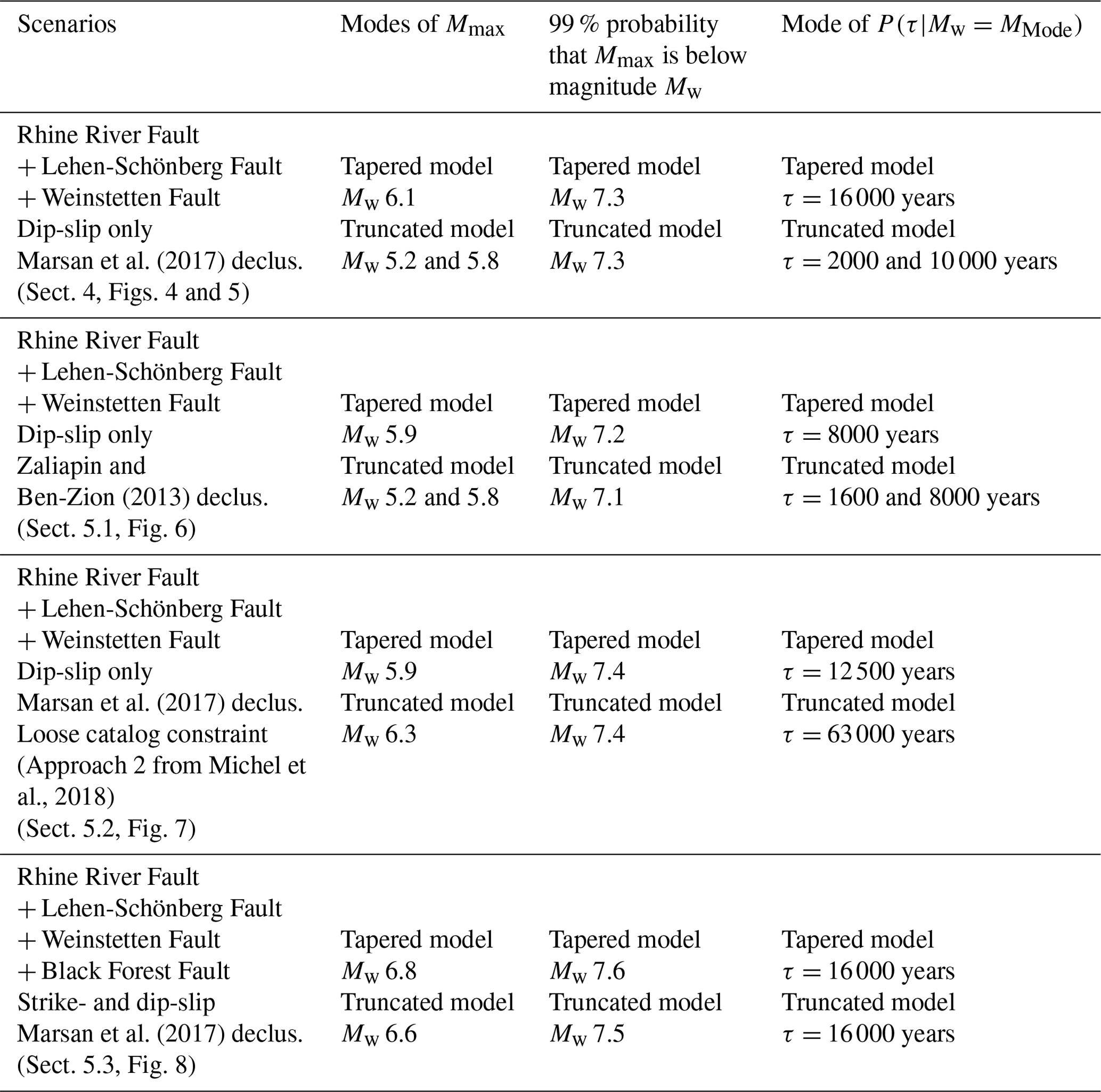
In any case, within this study, strong assumptions still had to be made that certainly affected the results. These include the methodology used to decluster the earthquake catalogs, determining whether it is wise to compare the loading rate of each fault with seismicity, opting to only consider the dip-slip component despite the fact that strike-slip is highly probable, covering the possibility of multi-segment ruptures and even the choice of the faults to be considered. Further work, from paleoseismology, seismic reflection, geodesy or earthquake relocation, is needed to obtain more information on the structures tectonically involved and their associated loading rates and to better constrain the URG seismic hazard.
The earthquake catalog has been made available by Drouet et al. (2020). The borehole temperature measurements are from Guillou-Frottier et al. (2013).
The analyses reported in this paper were done using MATLAB (The MathWorks Inc., 2023).
The supplement related to this article is available online at: https://doi.org/10.5194/nhess-24-163-2024-supplement.
SM, CD, LB and RJ conceptualized the study. SM performed the formal analysis with the help of JJ concerning the declustering of the seismicity catalogs. SM prepared and wrote the manuscript with contributions from all co-authors.
The contact author has declared that none of the authors has any competing interests.
Publisher's note: Copernicus Publications remains neutral with regard to jurisdictional claims made in the text, published maps, institutional affiliations, or any other geographical representation in this paper. While Copernicus Publications makes every effort to include appropriate place names, the final responsibility lies with the authors.
We thank the anonymous reviewers, who helped us improve our study.
This study was supported by the LRC Yves Rocard (Laboratoire de Recherche Conventionné CEA–ENS–CNRS) and received funding from the European Research Council (ERC) under the European Union's Horizon 2020 research and innovation program (Geo-4D project, grant no. 758210). Romain Jolivet received funding from the Institut Universitaire de France.
This paper was edited by Veronica Pazzi and reviewed by two anonymous referees.
Alwahedi, M. A. and Hawthorne, J. C.: Intermediate-Magnitude Postseismic Slip Follows Intermediate-Magnitude (M4 to 5) Earthquakes in California, Geophys. Res. Lett., 46, 3676–3687, https://doi.org/10.1029/2018GL081001, 2019.
Anderson, J. G. and Luco, J. E.: Consequences of slip rate constraints on earthquake occurrence relations, Bul. Seismol. Soc. Am., 73, 471–496, 1983.
Avouac, J.-P.: From Geodetic Imaging of Seismic and Aseismic Fault Slip to Dynamic Modeling of the Seismic Cycle, Annu. Rev. Earth Planet. Sci., 43, 233–271, https://doi.org/10.1146/annurev-earth-060614-105302, 2015.
Baize, S., Cushing, E. M., Lemeille, F., and Jomard, H.: Updated seismotectonic zoning scheme of Metropolitan France, with reference to geologic and seismotectonic data, Bull. Société Géologique Fr., 184, 225–259, https://doi.org/10.2113/gssgfbull.184.3.225, 2013.
Barth, A., Ritter, J. R. R., and Wenzel, F.: Spatial variations of earthquake occurrence and coseismic deformation in the Upper Rhine Graben, Central Europe, Tectonophysics, 651–652, 172–185, https://doi.org/10.1016/j.tecto.2015.04.004, 2015.
Baumont, D., Manchuel, K., Traversa, P., Durouchoux, C., Nayman, E., and Ameri, G.: Intensity predictive attenuation models calibrated in Mw for metropolitan France, Bull. Earthq. Eng., 16, 2285–2310, https://doi.org/10.1007/s10518-018-0344-6, 2018.
Beauval, C. and Bard, P.: History of probabilistic seismic hazard assessment studies and seismic zonations in mainland France, Comptes Rendus Géosci., 353, 413–440, https://doi.org/10.5802/crgeos.95, 2022.
Bertrand, G., Elsass, P., Wirsing, G., and Luz, A.: Quaternary faulting in the Upper Rhine Graben revealed by high-resolution multi-channel reflection seismic, Comptes Rendus Geosci., 338, 574–580, https://doi.org/10.1016/j.crte.2006.03.012, 2006.
Bettinelli, P., Avouac, J.-P., Flouzat, M., Bollinger, L., Ramillien, G., Rajaure, S., and Sapkota, S.: Seasonal variations of seismicity and geodetic strain in the Himalaya induced by surface hydrology, Earth Planet. Sc. Lett., 266, 332–344, https://doi.org/10.1016/j.epsl.2007.11.021, 2008.
Blanpied, M. L., Lockner, D. A., and Byerlee, J. D.: Frictional slip of granite at hydrothermal conditions, J. Geophys. Res.-Solid, 100, 13045–13064, https://doi.org/10.1029/95JB00862, 1995.
Bommer, J. J. and Crowley, H.: The Purpose and Definition of the Minimum Magnitude Limit in PSHA Calculations, Seismol. Res. Lett., 88, 1097–1106, https://doi.org/10.1785/0220170015, 2017.
Bonjer, K.-P.: Seismicity pattern and style of seismic faulting at the eastern borderfault of the southern Rhine Graben, Tectonophysics, 275, 41–69, https://doi.org/10.1016/S0040-1951(97)00015-2, 1997.
Calais, E., Camelbeeck, T., Stein, S., Liu, M., and Craig, T. J.: A new paradigm for large earthquakes in stable continental plate interiors, Geophys. Res. Lett., 43, 10621–10637, https://doi.org/10.1002/2016GL070815, 2016.
Cara, M., Cansi, Y., Schlupp, A., Arroucau, P., Béthoux, N., Beucler, E., Bruno, S., Calvet, M., Chevrot, S., Deboissy, A., Delouis, B., Denieul, M., Deschamps, A., Doubre, C., Fréchet, J., Godey, S., Golle, O., Grunberg, M., Guilbert, J., Haugmard, M., Jenatton, L., Lambotte, S., Leobal, D., Maron, C., Mendel, V., Merrer, S., Macquet, M., Mignan, A., Mocquet, A., Nicolas, M., Perrot, J., Potin, B., Sanchez, O., Santoire, J.-P., Sèbe, O., Sylvander, M., Thouvenot, F., Van Der Woerd, J., and Van Der Woerd, K.: SI-Hex: a new catalogue of instrumental seismicity for metropolitan France, Bull. Société Géologique Fr., 186, 3–19, https://doi.org/10.2113/gssgfbull.186.1.3, 2015.
Carter, N. L. and Hansen, F. D.: Creep of rocksalt, Tectonophysics, 92, 275–333, https://doi.org/10.1016/0040-1951(83)90200-7, 1983.
Chartier, T., Scotti, O., Clément, C., Jomard, H., and Baize, S.: Transposing an active fault database into a fault-based seismic hazard assessment for nuclear facilities – Part 2: Impact of fault parameter uncertainties on a site-specific PSHA exercise in the Upper Rhine Graben, eastern France, Nat. Hazards Earth Syst. Sci., 17, 1585–1593, https://doi.org/10.5194/nhess-17-1585-2017, 2017.
Churchill, R. M., Werner, M. J., Biggs, J., and Fagereng, Å.: Afterslip Moment Scaling and Variability From a Global Compilation of Estimates, J. Geophys. Res.-Solid, 127, e2021JB023897, https://doi.org/10.1029/2021JB023897, 2022.
Craig, T. J., Calais, E., Fleitout, L., Bollinger, L., and Scotti, O.: Evidence for the release of long-term tectonic strain stored in continental interiors through intraplate earthquakes, Geophys. Res. Lett., 43, 6826–6836, https://doi.org/10.1002/2016GL069359, 2016.
Craig, T. J., Chanard, K., and Calais, E.: Hydrologically-driven crustal stresses and seismicity in the New Madrid Seismic Zone, Nat. Commun., 8, 2143, https://doi.org/10.1038/s41467-017-01696-w, 2017.
Danciu, L., Nandan, S., Reyes, C., Basili, R., Weatherill, G., Beauval, C., Rovida, A., Vilanova, S., Şeşetyan, K., Bard, P.-Y., Cotton, F., Wiemer, S., and Giardini, D.: The 2020 update of the European Seismic Hazard Model: Model Overview, ETH Zürich, https://doi.org/10.3929/ethz-b-000590386, 2021.
Dieterich, J. H.: Modeling of Rock Friction Experimental Results and Constitutive Equations, J. Geophys. Res., 84, 2161–2168, https://doi.org/10.1029/JB084iB05p02161, 1979.
Doubre, C., Meghraoui, M., Masson, F., Lambotte, S., Jund, H., Bès de Berc, M., and Grunberg, M.: Seismotectonics in Northeastern France and neighboring regions, Comptes Rendus Géosci., 353, 153–185, https://doi.org/10.5802/crgeos.80, 2022.
Drouet, S., Ameri, G., Le Dortz, K., Secanell, R., and Senfaute, G.: A probabilistic seismic hazard map for the metropolitan France, Bull. Earthq. Eng., 18, 1865–1898, https://doi.org/10.1007/s10518-020-00790-7, 2020.
Fäh, D., Gisler, M., Jaggi, B., Kästli, P., Lutz, T., Masciadri, V., Matt, C., Mayer-Rosa, D., Rippmann, D., Schwarz-Zanetti, G., Tauber, G., and Wenk, T.: The 1356 Basel earthquake: an interdisciplinary revision, Geophys. J. Int., 178, 351–374, https://doi.org/10.1111/j.1365-246X.2009.04130.x, 2009.
Felzer, K. R.: Calculating California seismicity rates, Tech. Rep., US Geological Survey, https://doi.org/10.3133/ofr20071437I, 2008.
Freymark, J., Sippel, J., Scheck-Wenderoth, M., Bär, K., Stiller, M., Fritsche, J.-G., and Kracht, M.: The deep thermal field of the Upper Rhine Graben, Tectonophysics, 694, 114–129, https://doi.org/10.1016/j.tecto.2016.11.013, 2017.
Fuhrmann, T., Caro Cuenca, M., Knöpfler, A., van Leijen, F. J., Mayer, M., Westerhaus, M., Hanssen, R. F., and Heck, B.: Estimation of small surface displacements in the Upper Rhine Graben area from a combined analysis of PS-InSAR, levelling and GNSS data, Geophys. J. Int., 203, 614–631, https://doi.org/10.1093/gji/ggv328, 2015.
Grünthal, G., Stromeyer, D., Bosse, C., Cotton, F., and Bindi, D.: The probabilistic seismic hazard assessment of Germany – version 2016, considering the range of epistemic uncertainties and aleatory variability, Bull. Earthq. Eng., 16, 4339–4395, https://doi.org/10.1007/s10518-018-0315-y, 2018.
Guillou-Frottier, L., Carrė, C., Bourgine, B., Bouchot, V., and Genter, A.: Structure of hydrothermal convection in the Upper Rhine Graben as inferred from corrected temperature data and basin-scale numerical models, J. Volcanol. Geoth. Res., 256, 29–49, https://doi.org/10.1016/j.jvolgeores.2013.02.008, 2013.
Heidbach, O., Rajabi, M., Reiter, K., Ziegler, M. O., and WSM Team: World Stress Map Database Release 2016, V. 1.1, GFZ Data Services, https://doi.org/10.5880/WSM.2016.001, 2016.
Heidbach, O., Rajabi, M., Cui, X., Fuchs, K., Müller, B., Reinecker, J., Reiter, K., Tingay, M., Wenzel, F., Xie, F., Ziegler, M. O., Zoback, M.-L., and Zoback, M.: The World Stress Map database release 2016: Crustal stress pattern across scales, Tectonophysics, 744, 484–498, https://doi.org/10.1016/j.tecto.2018.07.007, 2018.
Henrion, E., Masson, F., Doubre, C., Ulrich, P., and Meghraoui, M.: Present-day deformation in the Upper Rhine Graben from GNSS data, Geophys. J. Int., 223, 599–611, https://doi.org/10.1093/gji/ggaa320, 2020.
Hinsken, S., Ustaszewski, K., and Wetzel, A.: Graben width controlling syn-rift sedimentation: the Palaeogene southern Upper Rhine Graben as an example, Int. J. Earth Sci., 96, 979–1002, https://doi.org/10.1007/s00531-006-0162-y, 2007.
Jomard, H., Cushing, E. M., Palumbo, L., Baize, S., David, C., and Chartier, T.: Transposing an active fault database into a seismic hazard fault model for nuclear facilities – Part 1: Building a database of potentially active faults (BDFA) for metropolitan France, Nat. Hazards Earth Syst. Sci., 17, 1573–1584, https://doi.org/10.5194/nhess-17-1573-2017, 2017.
Kraft, T. and Deichmann, N.: High-precision relocation and focal mechanism of the injection-induced seismicity at the Basel EGS, Geothermics, 52, 59–73, https://doi.org/10.1016/j.geothermics.2014.05.014, 2014.
Leonard, M.: Earthquake Fault Scaling: Self-Consistent Relating of Rupture Length, Width, Average Displacement, and Moment Release, Bull. Seismol. Soc. Am., 100, 1971–1988, https://doi.org/10.1785/0120090189, 2010.
Lutz, M., and Cleintuar, M.: Geological results of a hydrocarbon exploration campaign in the southern Upper Rhine Graben (Alsace Centrale, France), Bull. Angew. Geol., 4, 3–80, https://doi.org/10.5169/seals-221515, 1999.
Manchuel, K., Traversa, P., Baumont, D., Cara, M., Nayman, E., and Durouchoux, C.: The French seismic CATalogue (FCAT-17), Bull. Earthq. Eng., 16, 2227–2251, https://doi.org/10.1007/s10518-017-0236-1, 2018.
Marsan, D., Bouchon, M., Gardonio, B., Perfettini, H., Socquet, A., and Enescu, B.: Change in seismicity along the Japan trench, 1990–2011, and its relationship with seismic coupling, J. Geophys. Res.-Solid, 122, 4645–4659, https://doi.org/10.1002/2016JB013715, 2017.
Mayer-Rosa, D. and Cadiot, B.: A review of the 1356 Basel earthquake: Basic data, Tectonophysics, 53, 325–333, https://doi.org/10.1016/0040-1951(79)90077-5,1979.
Mazzotti, S., Aubagnac, C., Bollinger, L., Coca Oscanoa, K., Delouis, B., Do Paco, D., Doubre, C., Godano, M., Jomard, H., Larroque, C., Laurendeau, A., Masson, F., Sylvander, M., and Trilla, A.: FMHex20: An earthquake focal mechanism database for seismotectonic analyses in metropolitan France and bordering regions, BSGF – Earth Sci. Bull., 192, 10, https://doi.org/10.1051/bsgf/2020049, 2021.
Michel, S., Avouac, J.-P., Jolivet, R., and Wang, L.: Seismic and Aseismic Moment Budget and Implication for the Seismic Potential of the Parkfield Segment of the San Andreas Fault, Bull. Seismol. Soc. Am., 108, 19–38, https://doi.org/10.1785/0120160290, 2018.
Michel, S., Jolivet, R., Rollins, C., Jara, J., and Dal Zilio, L.: Seismogenic Potential of the Main Himalayan Thrust Constrained by Coupling Segmentation and Earthquake Scaling, Geophys. Res. Lett., 48, 1–10, https://doi.org/10.1029/2021GL093106, 2021.
Molnar, P.: Earthquake Recurrence Intervals and Plate Tectonics, Bull. Seismol. Soc. Am., 69, 115–133, https://doi.org/10.1785/BSSA0690010115, 1979.
Nivière, B., Bruestle, A., Bertrand, G., Carretier, S., Behrmann, J., and Gourry, J.-C.: Active tectonics of the southeastern Upper Rhine Graben, Freiburg area (Germany), Quaternary Sci. Rev., 27, 541–555, https://doi.org/10.1016/j.quascirev.2007.11.018, 2008.
Oleskevich, D. A., Hyndman, R. D., and Wang, K.: The updip and downdip limits to great subduction earthquakes: Thermal and structural models of Cascadia, south Alaska, SW Japan, and Chile, J. Geophys. Res.-Solid, 104, 14965–14991, https://doi.org/10.1029/1999JB900060, 1999.
Pena-Castellnou, S., Hürtgen, J., Baize, S., Preusser, F., Mueller, D., Jomard, H., Cushing, E. M., Rockwell, T. K., Seitz, G., Cinti, F. R., Ritter, J., and Reicherter, K.: Surface rupturing earthquakes along the eastern Rhine Graben Boundary Fault near Ettlingen-Oberweier (Germany), Tectonophysics, 869, 230114, https://doi.org/10.1016/j.tecto.2023.230114, 2023.
Rollins, C. and Avouac, J.-P.: A Geodesy- and Seismicity-Based Local Earthquake Likelihood Model for Central Los Angeles, Geophys. Res. Lett., 46, 3153–3162, https://doi.org/10.1029/2018GL080868, 2019.
Rotstein, Y. and Schaming, M.: The Upper Rhine Graben (URG) revisited: Miocene transtension and transpression account for the observed first-order structures, Tectonics, 30, 3, https://doi.org/10.1029/2010TC002767, 2011.
Rouland, D., Haessler, H., Bonjer, K. P., Gilg, B., Mayer-Rosa, D., and Pavoni, N.: The Sierentz Southern-Rhinegraben Earthquake of July 15, 1980. Preliminary Results, Dev. Solid Earth Geophys., 15, 441–446, https://doi.org/10.1016/B978-0-444-99662-6.50086-1, 1983.
Ruina, A.: Slip instability and state variable friction laws, J. Geophys. Res.-Solid, 88, 10359–10370, https://doi.org/10.1029/JB088iB12p10359, 1983.
Steer, P., Simoes, M., Cattin, R., and Shyu, J. B. H.: Erosion influences the seismicity of active thrust faults, Nat. Commun., 5, 5564, https://doi.org/10.1038/ncomms6564, 2014.
Stirling, M., Goded, T., Berryman, K., and Litchfield, N.: Selection of Earthquake Scaling Relationships for Seismic-Hazard Analysis, Bull. Seismol. Soc. Am., 103, 2993–3011, https://doi.org/10.1785/0120130052, 2013.
Stucchi, M., Rovida, A., Gomez Capera, A. A., Alexandre, P., Camelbeeck, T., Demircioglu, M. B., Gasperini, P., Kouskouna, V., Musson, R. M. W., Radulian, M., Sesetyan, K., Vilanova, S., Baumont, D., Bungum, H., Fäh, D., Lenhardt, W., Makropoulos, K., Martinez Solares, J. M., Scotti, O., Živčić, M., Albini, P., Batllo, J., Papaioannou, C., Tatevossian, R., Locati, M., Meletti, C., Viganò, D. and Giardini, D.: The SHARE European Earthquake Catalogue (SHEEC) 1000–1899, J. Seismol., 17, 523–544, https://doi.org/10.1007/s10950-012-9335-2, 2013.
The MathWorks Inc.: MATLAB version: 9.14.0.2239454 (R2023a) Update 1, The MathWorks Inc., Natick, Massachusetts, https://www.mathworks.com (last access: 19 January 2024), 2023.
Traversa, P., Baumont, D., Manchuel, K., Nayman, E., and Durouchoux, C.: Exploration tree approach to estimate historical earthquakes Mw and depth, test cases from the French past seismicity, Bull. Earthq. Eng., 16, 2169–2193, https://doi.org/10.1007/s10518-017-0178-7, 2018.
Wells, D. L. and Coppersmith, K. J.: New empirical relationships among magnitude, rupture length, rupture width, rupture area, and surface displacement, Bull. Seismol. Soc. Am., 84, 974–1002, https://doi.org/10.1785/BSSA0840040974, 1994.
Weng, H. and Yang, H.: Seismogenic width controls aspect ratios of earthquake ruptures, Geophys. Res. Lett., 44, 2725–2732, https://doi.org/10.1002/2016GL072168, 2017.
Wesnousky, S. G.: Predicting the endpoints of earthquake ruptures, Nature, 444, 358–360, https://doi.org/10.1038/nature05275, 2006.
Woessner, J., Laurentiu, D., Giardini, D., Crowley, H., Cotton, F., Grünthal, G., Valensise, G., Arvidsson, R., Basili, R., Demircioglu, M. B., Hiemer, S., Carlo Meletti, C., Musson, R. W., Rovida, A. N., Sesetyan, K., Stucchi, M., and SHARE consortium: The 2013 European Seismic Hazard Model: key components and results, Bull. Earthq. Eng., 13, 3553–3596, https://doi.org/10.1007/s10518-015-9795-1, 2015.
Zaliapin, I. and Ben-Zion, Y.: Earthquake clusters in southern California I: Identification and stability, J. Geophys. Res.-Solid, 118, 2847–2864, https://doi.org/10.1002/jgrb.50179, 2013.