Total water levels along the South Atlantic Bight during three along-shelf propagating tropical cyclones: relative contributions of storm surge and wave runup

Total water levels (TWLs), including the contribution of wind waves, associated with tropical cyclones (TCs) are among the most damaging hazards faced by coastal communities. TC-induced economic losses are expected to increase because of stronger TC intensity, sea level rise, and increased populations along the coasts. TC intensity, translation speed, and distance to the coast affect the magnitude and duration of increased TWLs and wind waves. Under climate change, the proportion of high-intensity TCs is projected to increase globally, whereas the variation pattern of TC translation speed also depends on the ocean basin and latitude. There is an urgent need to improve our understanding of the linkages between TC characteristics and TWL components. In the past few years, hurricanes Matthew (2016), Dorian (2019), and Isaias (2020) propagated over the South Atlantic Bight (SAB) with similar paths but resulted in different coastal impacts. We combined in situ observations and numerical simulations with the Coupled Ocean–Atmosphere–Wave–Sediment Transport (COAWST) modeling system to analyze the extreme TWLs under the three TCs. Model verification showed that the TWL components were well reproduced by the present model setup. Our results showed that the peak storm surge and the peak wave runup depended mainly on the TC intensity, the distance to the TC eye, and the TC heading direction. A decrease in TC translation speed primarily led to longer exceedance durations of TWLs, which may result in more severe economic losses. Wave-dependent water level components (i.e., wave setup and wave swash) were found to dominate the peak TWL within the near-TC field. Our results also showed that in specific conditions, the prestorm wave runup associated with the TC-induced swell may lead to TWLs higher than at the peak of the storm. This was the case along the SAB during Hurricane Isaias. Isaias's fast TC translation speed and the fact that its swell was not blocked by any islands were the main factors contributing to these peak TWLs ahead of the storm peak.

1 Introduction

Total water levels (TWLs), defined as the combination of astronomic tides, mean sea level, storm surge, and wave runup (combination of wave setup and wave swash), associated with tropical cyclones (TCs) are among the leading hazards faced by coastal communities (e.g., Kalourazi et al., 2020; Sallenger, 2000). The Saffir–Simpson Hurricane Wind Scale (SSHWS) has been used to estimate the potential impacts and economic losses caused by TCs based on the maximum sustained wind speed. However, the maximum sustained wind speed, the TC translation speed (Liu et al., 2007; Xu et al., 2007), the size of the storm (Irish et al., 2008), and the storm track (Suh and Lee, 2018; Wang et al., 2020) affect wave heights, wave periods, and storm surge levels along the coast differently. Alipour et al. (2022) pointed out that using SSHWS as a proxy of the expected impacts alone may lead to severe miscalculation, and they proposed a new scaling system associated with rainfall, storm surge, and wind speed. Irish and Resio (2010) proposed a hydrodynamic-based surge scale for hurricane surge hazard and an approach for predicting expected flood inundation and economic losses. Sallenger (2000) proposed a more complex approach in which the TWL relative to the dune crest (D_crest) and dune base (D_base) elevations was used to classify four expected morphological impact regimes: swash (TWL < D_base), collision (D_base≤ TWL < D_crest), and overwash and inundation (D_crest ≤ TWL). In the overwash regime TWL exceeds D_crest when the wave swash effects are accounted for. In the inundation regime TWL exceeds D_crest even without the effect of the wave swash. Among these regimes, coastal dunes experience the direct impacts of surf-zone processes in the inundation regime, when TWL exceeds D_crest. Thus, the inundation regime is expected to induce the highest economic losses among the four impact regimes, while the swash regime represents the least severe condition with less anticipated economic losses. TWL thus represents the combination of storm-independent (the mean sea level and astronomic tides) and storm-dependent (wave runup and storm surge) water level components, being a better indicator of the increased water levels than the storm surge alone (Stockdon et al., 2007). We assume that astronomic tides and storms are at first order independent, although extreme winds and storm surges can interact with the tidal wave and cause tidal distortions (e.g., Paniagua-Arroyave et al., 2019). The wave runup is a wind-wave-dependent parameter composed by a wave-averaged sea level variation known as “wave setup” and a wave-varying fluctuating component known as “wave swash” (Stockdon et al., 2006). Previous efforts have shown the complexity and uncertainty of TC-induced surges and compound floods. However, the response of TWL to storm characteristics is more complicated than that corresponding to the storm surge, and the relative role of the wave runup and storm surge and the dependency on storm characteristics are still poorly understood.

There are primarily two approaches for computing TWLs during extreme storms: with numerical models (e.g., Hegermiller et al., 2019) and with observed water levels and waves (e.g., Serafin and Ruggiero, 2014). For example, η₀ (i.e., the sum of astronomic tides, mean sea level, and storm surge) observations were available at National Oceanic and Atmospheric Administration (NOAA; https://tidesandcurrents.noaa.gov/, last access: 28 August 2023) tide gauges. Coupled ocean–wave modeling systems such as the Coupled Ocean–Atmosphere–Wave–Sediment Transport model (COAWST; Warner et al., 2010) can also be applied to predict η₀ deterministically and probabilistically. However, the wave runup component needed to compute the TWL is not captured by tide gauges, and regional ocean models usually do not have sufficient spatial resolution to reproduce the wave setup accurately. Moreover, due to the use of phase-averaged models, coupled modeling systems such as the Regional Ocean Modeling System–Simulating WAves Nearshore (ROMS–SWAN) are not able to reproduce the wave swash component. While models such as the Infragravity Wave (InWave) model installed within COAWST (Olabarrieta et al., 2023) can solve infragravity waves, phase-resolving models like FUNWAVE (Shi et al., 2012) can be applied to simulate the wave swash. However, InWave and FUNWAVE require higher resolution in space and time, which makes them relatively inefficient for large spatial areas.

To overcome this modeling challenge, the wave runup can be computed using empirical formulas and linearly added to η₀. For example, Serafin and Ruggiero (2014) applied the empirical formula proposed by Stockdon et al. (2006) to compute the wave runup at NOAA tide gauges using the wave parameters observed at nearby National Data Buoy Center (NDBC; https://www.ndbc.noaa.gov/, last access: 28 August 2023) wave buoys along the US West Coast. While the wave runup of Stockdon et al.'s (2006) formulation is represented by a linear increase with increasing deep-water zero-order moment wave height (H₀), Senechal et al. (2011) suggested an upper limit of wave runup at highly dissipative beaches under energetic conditions (e.g., tropical cyclone). Senechal et al. (2011) proposed another empirical formula for wave runup based on wave height alone, to avoid the overprediction under such scenarios, and stated that the saturation of wave runup required further studies and measurements under diverse beach scenarios before generalization. Despite the importance of the wave runup in TWL estimation, the sensitivity of wave runup to the choice of these formulas had not been thoroughly examined. In the meantime, the sensitivity and the applicability of these formulas under different storm conditions are poorly understood.

Parker et al. (2023) recently characterized the relative contributions of astronomic tides, storm surge, and wave setup to extreme water levels along the US Southeast Coast, discovering regional patterns in the average contributions of waves and storm surge to extreme water levels over the 38-year hindcast. Here, we analyzed how TC characteristics affect the relative contributions of storm surge and wave runup to TWLs and their impacts by applying the COAWST modeling system to simulate TWLs along the South Atlantic Bight (SAB; extending from North Carolina to Florida) during three historical TCs with similar tracks. In the recent past, three hurricanes – Matthew (2016), Dorian (2019), and Isaias (2020) – propagated through the shelf of the SAB with similar tracks (Fig. 1). The average TC characteristics and the associated economic losses of these three TCs according to the International Best Track Archive for Climate Stewardship (IBTrACS; Knapp et al., 2018, 2010) are indicated in Table 1. While the economic loss from Matthew (USD 10.0 billion; Stewart, 2017) was the highest of all storms, it was 1 order of magnitude higher than that of Dorian (USD 1.6 billion by Dorian; Avila et al., 2020), even with similar maximum sustained wind speeds (V_max). Surprisingly, while Dorian had a stronger intensity than Isaias according to the SSHWS, Isaias caused higher economic loss (USD 4.8 billion; Latto et al., 2021). Isaias had the fastest translation speed (V_t) across all three hurricanes within the SAB, whereas Dorian had the slowest V_t and the smallest radius of maximum wind (R_max) on average. How the differences in V_max, V_t, and distance to the coast influenced the TWL components during these three TCs is still not well understood. With similar tracks over the SAB, these three historical TCs provided the opportunity to determine the effects of each TC property on waves and TWL along the coast. Because the proportion of high-intensity TCs (i.e., SSHWS category 4 to 5) and the corresponding maximum sustained wind are projected to increase at the global scale (Masson-Delmotte et al., 2021) due to climate change, understanding how TC characteristics influence the makeup of the TWL is essential for preparing for future coastal impacts.

Table 1 Averaged values of TC parameters of the three historical hurricanes within the SAB. The values were calculated from the International Best Track Archive for Climate Stewardship (IBTrACS) and National Hurricane Center datasets. V_t is the translation speed of storms, V_max is the maximum sustained wind, P_min is the minimum atmosphere pressure, and R_max is the radius of maximum wind; economic loss is estimated in billion USD.

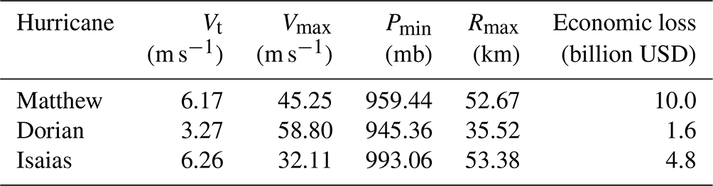
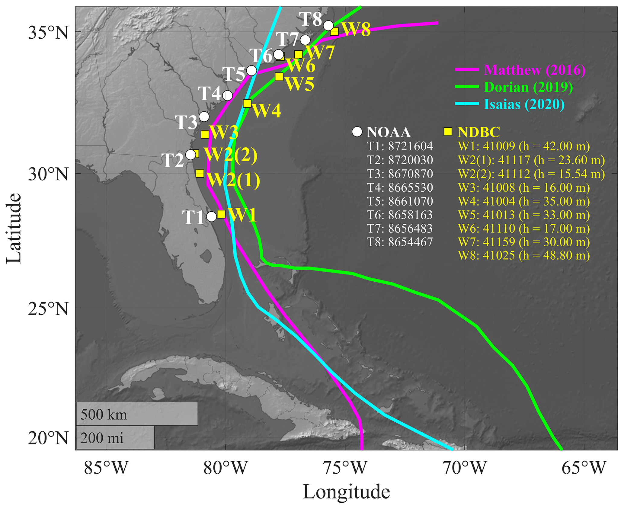
Figure 1 Best tracks of hurricanes Matthew (2016; magenta), Dorian (2019; green), and Isaias (2020; cyan); NOAA tide gauges (white circles); and NDBC wave buoys (yellow squares) selected for the model verification. h represents the water depth.

This paper is organized as follows: a brief review of the modeling system and model setup is presented following the Introduction. Model verification based on the comparison with historical observations at eight NOAA tide gauges can be found next. TWL components along the SAB during Matthew (2016), Dorian (2019), and Isaias (2020) are analyzed and compared in the “Results and discussion” section. The applicability of the two empirical wave runup formulas and the effect of TC characteristics on wave runup are also discussed and presented.

2 Methods

Following the modeling framework of Hegermiller et al. (2019), we configured COAWST as a coupled ocean–wave model and set it up to simulate the ocean and wave dynamics during hurricanes Matthew (2016), Dorian (2019), and Isaias (2020). Ocean dynamics were resolved with the ROMS (Shchepetkin and McWilliams, 2005), while wind wave generation and propagation were simulated with SWAN (Booij et al., 1999). The computational flowchart of the ocean circulation–wave coupling applied here is shown in the Appendix (Fig. A1). The ocean and wave models used the same horizontal grids, with a 5 km resolution parent grid covering the entire US East Coast and a 1 km resolution child grid covering the southern SAB.

2.1 Ocean model (ROMS)

ROMS solves the Reynolds-averaged Navier–Stokes (RANS) equations utilizing a three-dimensional terrain-following framework with a curvilinear coordinate transformation and finite-difference approximations (Shchepetkin and McWilliams, 2005). Additional information on the wave–current closure models included in ROMS is provided in Kumar et al. (2012) and Warner et al. (2008, 2010).

2.2 Wave model (SWAN)

The third-generation spectral wave model SWAN (Booij et al., 1999) solves the wave action evolution while considering refraction, shoaling, wave–current interactions, wind–wave generation, and varied wave energy dissipation (bottom friction, breaking, and white-capping). The semi-empirical formula derived from the JOint North Sea WAve Project (JONSWAP) was used to calculate bottom friction (Hasselmann et al., 1973). We calculated wind wave growth and white-capping using the formulas presented by Komen et al. (1984). We used discrete interaction approximation (DIA; Hasselmann et al., 1985) for the nonlinear quadruplet wave–wave interactions.

2.3 Model setup

In the current work, winds, atmospheric pressure, relative humidity, and surface air temperature from the RAPid refresh (RAP) reanalyzed data (Benjamin et al., 2016; https://www.nco.ncep.noaa.gov/pmb/products/rap/, last access: 18 August 2023) were employed to force ROMS. This dataset comprised atmospheric pressure at mean sea level (MSL) and wind speeds at 10 m above mean sea level. Although RAP only covers a portion of the computational domain, it has a spatial resolution of 13 km at hourly time intervals. The Global Forecast System (GFS; 50 km resolution with a 3 h time interval; https://www.ncdc.noaa.gov/data-access/model-data/model-datasets/global-forcast-system-gfs, last access: 18 August 2023) provided wind and atmospheric pressure forces for offshore regions that RAP did not cover.

The US East Coast domain had a horizontal grid resolution of 5 km with 896 (ξ direction) × 336 (η direction) grid cells. The SAB domain had a horizontal grid resolution of 1 km with 272 (ξ direction) × 376 (η direction) grid cells. The numerical grids of ROMS had 16 vertical layers. For the SAB grid and the US East Coast grid, the baroclinic time steps in ROMS were 30 and 15 s, respectively. To determine the initial conditions for the surface water levels, velocities, salinity, and temperature, we used the reanalyzed data from the HYbrid Coordinate Ocean Model (HYCOM; Metzger et al., 2014; https://www.ncei.noaa.gov/thredds-coastal/catalog/hycom_region1/catalog.html, last access: 31 March 2023). A total of 13 tidal elements (M2, S2, N2, K1, K2, O1, P1, Q1, MF, MM, M4, MS4, and MN4) from the TPXO tide model database at Oregon State University (Egbert and Erofeeva, 2002) were applied to the parent grid to simulate astronomic tides. The Flather boundary condition (Flather, 1976) was applied at the boundaries of the ROMS model (the northeast and southeast boundaries of the dashed black box in panel a of Fig. A2) for the momentum balance to radiate out deviations from exterior values at the speed of the external ocean waves. A 2 d spinup was done, followed by an 11 d simulation (i.e., 13 d in total). The initial conditions, such as currents, water levels, temperature, and salinity, were examined to show that the 2 d spinup is adequate for them to achieve the equilibrium state in the model. It was determined that an 11 d simulation period, including at least 5 d prior to the storm's peak, was sufficient to track the development and spread of swells near the SAB.

For the boundary conditions of the SWAN model for Hurricane Matthew, hourly statistical wave bulk parameters (zero-order moment wave height, mean wave direction, and peak wave period) from NOAA's WAVEWATCH III reanalyzed global dataset (The WAVEWATCH III Development Group, 2016; https://polar.ncep.noaa.gov/waves/ensemble/download.shtml, last access: 31 March 2023) were imposed at 47 boundary segments along the southeast and northeast boundaries of the US East Coast grid (the dashed black box in Fig. A2) assuming the JONSWAP wave spectra. NOAA's WAVEWATCH III reanalyzed global dataset did not have available data during Dorian and Isaias. Thus, we employed a larger grid to cover the North Atlantic Ocean and the Gulf of Mexico with our modeling system to generate the wave boundary conditions for these two TCs for input as boundary conditions to the SWAN model. Wave spectrum was solved with 60 and 25 directional and frequency bins. The parent and child grids were solved with 30 and 15 s as their computational time steps, respectively. As for the atmospheric forcing, SWAN used the same GFS–RAP input as ROMS.

Using the Model Coupling Toolkit, water levels, current velocities, and wave fields are two-way coupled in COAWST (Warner et al., 2008). In our simulations, the data exchange interval between ROMS and SWAN was set to 30 min, including water surface elevation, current velocities, and statistical wave bulk parameters (e.g., zero-order moment wave heights, peak and mean wavelengths, peak and mean wave periods, peak and mean wave directions, and wave dissipation). This exchange interval has been tested and used by Hegermiller et al. (2019) and Hsu et al. (2023), in which the nearshore hydrodynamics were replicated adequately. Thereby, we applied the same data exchange interval in the present work. Specifics regarding the coupling method and an example case study were provided (Warner et al., 2008, 2010). The wind shear stresses and sea surface roughness by Taylor and Yelland (2001) at the sea surface were computed and used to force the ocean model. The vortex–force formulation (Kumar et al., 2012; Uchiyama et al., 2010) was employed in the current study to account for wave–current interaction. Furthermore, the wave and current boundary layer properties were estimated with the SSW_BBL option, which used the model of Madsen (1994).

2.4 Empirical formulas for wave runup

We followed the work of Serafin and Ruggiero (2014) and applied the empirical formulas proposed by Stockdon et al. (2006) and Senechal et al. (2011) to compute the wave runup at NOAA tide gauges using the wave parameters at nearby NDBC wave buoys along the SAB. The locations of the tide gauges and wave buoys are indicated in Fig. 1. The empirical formula proposed by Stockdon et al. (2006) (Eqs. 1 and 2) provides the 2 % exceedance percentile of extreme wave runup (R₂):

$$\begin{array}{}\text{(1)}& {\displaystyle }\begin{array}{rl}{R}_{\mathrm{2}}& =\mathrm{1.1}\left(\mathrm{0.35}{\mathit{\beta }}_{\mathrm{f}}{\left(H_{\mathrm{0}}{L}_{\mathrm{0}}\right)}^{\frac{\mathrm{1}}{\mathrm{2}}}+{\displaystyle \frac{{\left[H_{\mathrm{0}}{L}_{\mathrm{0}}\left(\mathrm{0.563}{\mathit{\beta }}_{\mathrm{f}}^{\mathrm{2}}+\mathrm{0.004}\right)\right]}^{\frac{\mathrm{1}}{\mathrm{2}}}}{\mathrm{2}}}\right),\\ & \mathrm{0.3}\le {\mathit{\xi }}_{\mathrm{0}}<\mathrm{4.0},\end{array}\text{(2)}& {\displaystyle }{R}_{\mathrm{2}}=\mathrm{0.043}{\left(H_{\mathrm{0}}{L}_{\mathrm{0}}\right)}^{\frac{\mathrm{1}}{\mathrm{2}}},{\mathit{\xi }}_{\mathrm{0}}<\mathrm{0.3},\end{array}$$

in which the foreshore beach slope (β_f) and deep-water wave parameters (H₀ is the deep-water zero-order moment wave height, and L₀ is the deep-water peak wavelength) and the Iribarren number (ξ₀) (Eq. 3) were required. ξ₀ was used to categorize wave breaker types (Battjes, 1974). In Eq. (1), the first part ($\mathrm{1.1}\cdot \mathrm{0.35}{\mathit{\beta }}_{\mathrm{f}}{\left(H_{\mathrm{0}}{L}_{\mathrm{0}}\right)}^{\frac{\mathrm{1}}{\mathrm{2}}}$) represents wave setup, and the second part $\left(\mathrm{1.1}\cdot \frac{{\left[H_{\mathrm{0}}{L}_{\mathrm{0}}\left(\mathrm{0.563}{\mathit{\beta }}_{\mathrm{f}}^{\mathrm{2}}+\mathrm{0.004}\right)\right]}^{\frac{\mathrm{1}}{\mathrm{2}}}}{\mathrm{2}}\right)$ represents the combination of infragravity swash and incident swash.

$$\begin{array}{}\text{(3)}& {\mathit{\xi }}_{\mathrm{0}}={\displaystyle \frac{{\mathit{\beta }}_{\mathrm{f}}}{{\left(H_{\mathrm{0}}/L_{\mathrm{0}}\right)}^{\mathrm{1}/\mathrm{2}}}}\end{array}$$

While beach slopes depend on local coastal morphology, wave heights and wavelengths also depend on storm characteristics. Stockdon et al. (2007) pointed out that the swash zone can be moved onshore along the beach profile due to the large waves and storm surges during extreme weather. Consequently, the mean beach slope (β_m), measuring the slope of the beach from the shoreline to the dune base, was suggested and defined as the relevant slope in Eqs. (1) and (3) during hurricanes. The deep-water wave parameters can be calculated by de-shoaling the waves from a given point along the coast or shelf to deep water using the linear wave theory. The empirical formula developed by Stockdon et al. (2006) separated intermediate to wave-reflective beach scenarios (0.3 < ξ₀ < 4.0, Eq. 1) from extremely dissipative conditions (ξ₀ < 0.3, Eq. 2). According to their dataset, R₂ under ξ₀ < 0.3 did not necessarily linearly depend on the beach slope and was generally dominated by infragravity waves. Thus, Stockdon et al. (2006) suggested that a parameterization with a similar form for infragravity swash should be used to model the R₂ under ξ₀ < 0.3 (Eq. 2). While the field data employed by Stockdon et al. (2006) did not specifically include highly energetic conditions during storms, Stockdon et al. (2014) compared the numerical simulated wave runup of XBeach (Roelvink et al., 2009) with the parameterized wave runup of Stockdon et al. (2006) under storm conditions. Stockdon et al. (2014) showed that the parameterized wave runups were consistent with XBeach model results for the SSHWS category 1 scenario, while the wave runups associated with more energetic conditions still require further discussions.

While R₂ in the Stockdon et al. (2006) formulation is represented by a linear increase with increasing H₀, Senechal et al. (2011) suggested an upper limit of R₂ at highly dissipative beaches under energetic conditions (e.g., tropical cyclone). Senechal et al. (2011) proposed another empirical formula for R₂ based on H₀ alone (Eq. 4) to avoid the overprediction under such scenarios.

$$\begin{array}{}\text{(4)}& R_{\mathrm{2}}=\mathrm{2.14}\tan h\left(\mathrm{0.4}{H}_{\mathrm{0}}\right)\end{array}$$

While the observed data used in Stockdon et al. (2006) included part of the study area of the present work (i.e., North Carolina), most of the scenarios (> 93 %) at the peaks of hurricanes Matthew, Dorian, and Isaias along the SAB belonged to intermediate beach conditions, which Stockdon et al. (2006) primarily focused on (0.3 < ξ₀ < 4.0). On the contrary, Senechal et al. (2011) specifically considered dissipative beach conditions.

3 Model verification

We used the observed data from eight NOAA tide gauges and nine NDBC buoys along the SAB to verify the model performance (Fig. 1). These NOAA tide gauges and NDBC buoys were selected based on the observed data availability during the three hurricanes. Tide gauges T1, T7, and T8 are installed behind a barrier island, while tide gauge T2 is installed within an estuary. The other four tide gauges are installed at piers on local beaches. Thus, the measured TWLs at T1, T2, T7, and T8 may not reflect the exact water levels at the beach. The model performance on statistical wave bulk parameters (zero-order moment wave height, mean wave direction, and peak wave period) and the wave energy spectra resulting from the current model setup have been verified and discussed by Hsu et al. (2023). In the present study, we followed the approach of Serafin and Ruggiero (2014) to compute TWLs, including wave runup (R₂), and used the measurements at NOAA tide gauges (T1–T8) and the nearby NDBC wave buoys (W1–W8) as the “observational data”. While seven of these NOAA tide gauges had corresponding NDBC buoys used for wave runup estimation, two NDBC buoys (W2(1) and W2(2)) were assigned to the tide gauge T2 (NOAA 8720030) for different storm events due to the lack of data. Wave parameters (zero-order moment wave height, H_m0, and peak wave period, T_P) at W1–W8 were used to estimate the corresponding R₂ at T1–T8 using the formula of Stockdon et al. (2006). We used the linear wave dispersion relation to compute the representative deep-water peak wave parameters (H₀ and L₀). For model results, we used the predicted H_m0 and T_P extracted at the COAWST computational grid with the shortest distance to the U.S. Geological Survey (USGS; https://coastal.er.usgs.gov/data-release/doi-F7GF0S0Z/, last access: 31 March 2023) data points along the SAB. The mean beach slopes measured by USGS before Hurricane Matthew along the SAB (Doran et al., 2015, 2017) were used to compute R₂ (Eq. 1). While USGS had some post-Matthew field surveys, these later measurements only covered a relatively small range or did not overlap with the SAB. To simplify the problem and to focus on the comparison of TC-induced water level components under the three historical TCs, the coastal morphology was assumed not to change between storms.

To quantify the model performance, we used the correlation coefficient between the “measured” and simulated peak storm surge, peak wave runup, and maximum continuous duration of TWL ≥D_base at these eight NOAA tide gauges (Fig. 2). Overall, model results showed good agreement with NOAA observations: from the 24 data points at eight NOAA tide gauges during three storms with the correlation coefficient higher than 0.7 for the peak TWL, the peak storm surge (η_S), the peak wave runup (R₂), and the maximum continuous duration of TWL ≥D_base(T_TWL). We utilized the Lanczos low-pass filter (Duchon, 1979) to remove the astronomic tides from η₀ and obtained the storm surge (η_S). It is noted that there were larger discrepancies in the peak η_S and T_TWL. There may be several reasons causing the discrepancy between observed and model results. For example, the observed data at NOAA tide gauges may not reflect the actual extreme water levels and the corresponding durations at the beach because of their locations, especially at tide gauges T1, T2, T7, and T8, which are located within estuaries or behind barrier islands. The current spatial resolution of the computational grid may not completely reflect the details of the bathymetry around these estuaries and narrow barrier islands. Secondly, the potential influence of rainfall and river discharge nearby these observed locations may also contribute to the TWL. As we used a low-pass filter to remove the contribution from astronomic tides, rainfall and river discharge may contribute to the resulting water level as well. Accordingly, we used the model results from the ROMS–SWAN model to focus on the storm-forced water level components induced by wind and atmospheric pressure at beaches along the SAB in the present work, which also allows for a higher spatial and temporal resolution of TWL at the beach.

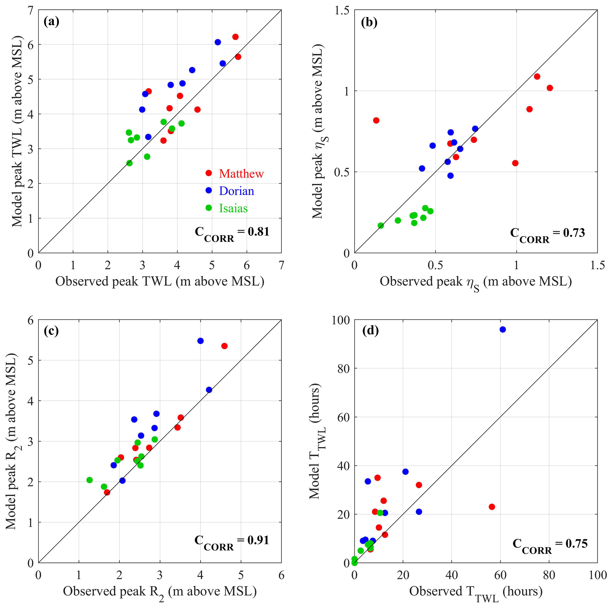
Figure 2 Model verification of (a) the peak TWLs, (b) the peak storm surge, (c) the peak wave runup, and (d) the maximum continuous duration of TWL ≥D_base(T_TWL) at eight NOAA tide gauges during the three historical hurricanes. The red, blue, and green points denote the data of hurricanes Matthew, Dorian, and Isaias, respectively. The corresponding correlation coefficients (C_CORR) are shown in the bottom-right corner in each panel.

4 Results and discussion

This section compares the temporal and spatial changes in η_S and R₂ along the SAB caused by hurricanes Matthew in 2016, Dorian in 2019, and Isaias in 2020. Additionally, the relationship between TC characteristics and the TC-induced water level components is examined.

4.1 Storm-forced water level components

TWL depends on the astronomic tides, which is at first order independent of TC characteristics, in such a way that the peak of the TC-induced water level can occur at any tidal level. Here, we focused on the influences of V_max, V_t, and TC path on two TC-induced water level components: η_S and R₂. We combined η_S with the R₂ estimated by the Stockdon et al. (2006) formulation to obtain the peak TC-induced water level, η_T (panels a1, b1, and c1 in Fig. 3).

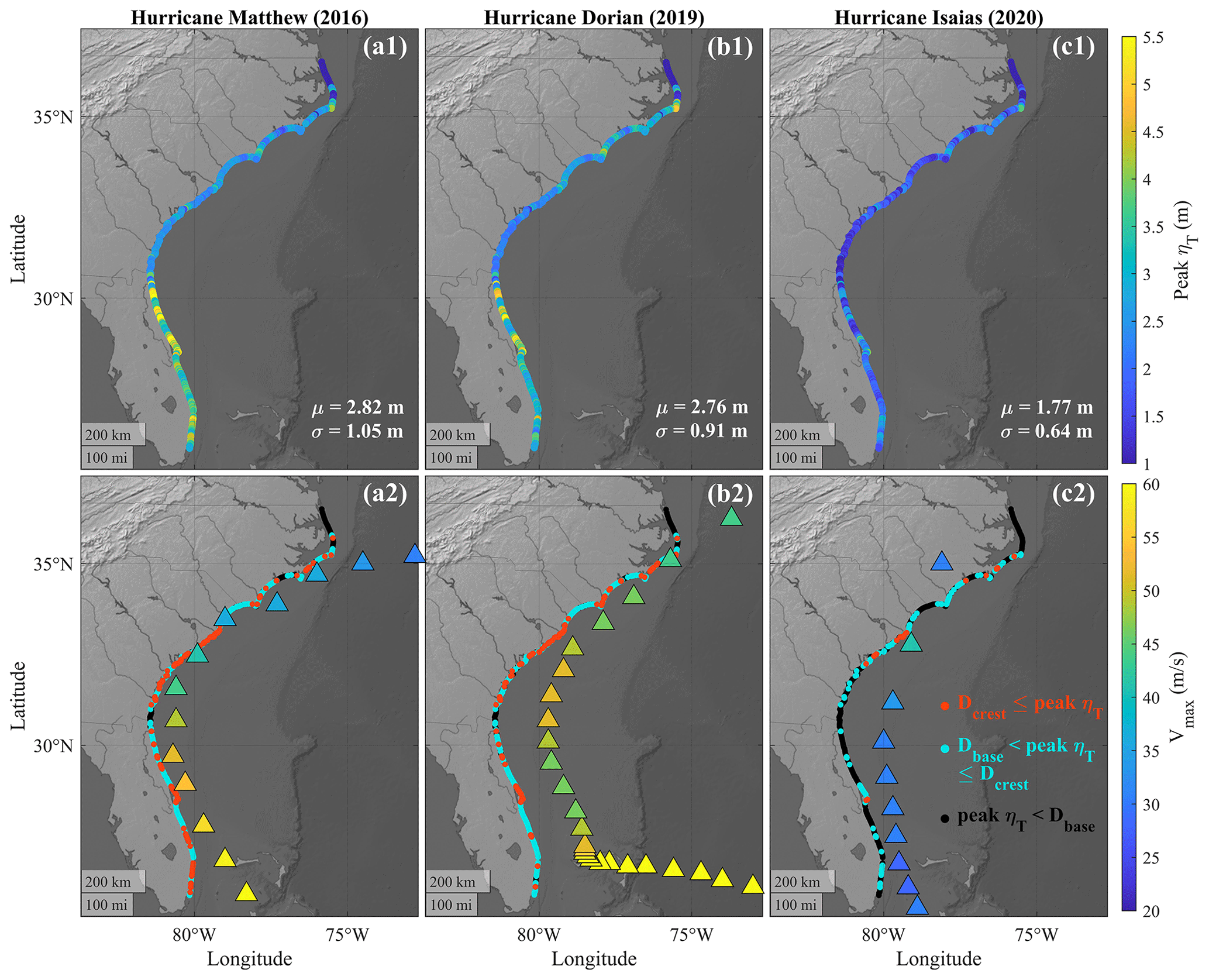
Figure 3 (a1, b1, c1) Peak η_T (i.e., the sum of η_S and R₂) along the SAB during the three hurricanes; μ represents the average, and σ is the standard deviation along the SAB. (a2, b2, c2) IBTrACS data of the TC every 6 h with the color map presenting instantaneous maximum sustained wind (V_max); the red, blue, and black points indicate the most severe levels achieved during the TC. We followed Sallenger (2000) and used local D_crest and D_base elevations to categorize the peak η_T. These categorizations are D_crest ≤ peak η_T, D_base ≤ peak η_T < D_crest, and peak η_T < D_base.

4.2 Peak values and durations of η_T and TWL over specified thresholds along the SAB

Matthew and Dorian had stronger V_max on average (45.25 and 58.80 m s⁻¹, respectively) within the SAB compared to Isaias (32.11 m s⁻¹; Table 1), which led to lower surge levels during Isaias (15 to 90 cm lower than Matthew and Dorian). Meanwhile, Matthew's distance to the coastline (47.38 km) was shorter compared to Dorian (96.73 km) and Isaias (97.24 km) along the SAB on average. The peak η_T along the SAB showed similar values and distribution patterns during Matthew and Dorian but was 60 % to 65 % smaller on average during Isaias (panels a1, b1, and c1 in Fig. 3). Along Florida's southeast coast the peak η_T was higher during Matthew compared to Dorian and Isaias but decreased significantly along Georgia and South Carolina as Matthew propagated northward and weakened. This led to a higher deviation of peak η_T along the SAB during Matthew compared to Dorian and Isaias.

We used D_crest and D_base as thresholds to categorize the peak η_T and TWL into the impact regimes of Sallenger (2000) along the SAB. The peak η_T can occur coincidently with either the high tide or the low tide. Without the astronomic tides, the present work isolated and determined the contribution of TC-induced water level components and its dependency on TC characteristics. While Sallenger (2000) used the thresholds to categorize the morphological impacts caused by the TWLs, we utilized the thresholds to categorize the levels of TC-induced water levels (η_T) specifically. A total of 23.0 % and 19.9 % of the coastal sites experienced peak η_T≥D_crest (red points in panels a2, b2, and c2 of Fig. 3) during Matthew and Dorian, respectively. These percentages were higher during Matthew and Dorian compared to those during Isaias (3.5 %) (Table 2).

Table 2 Percentage of coastal sites of each categorization of peak η_T and peak TWL during the three historical TCs along the SAB.

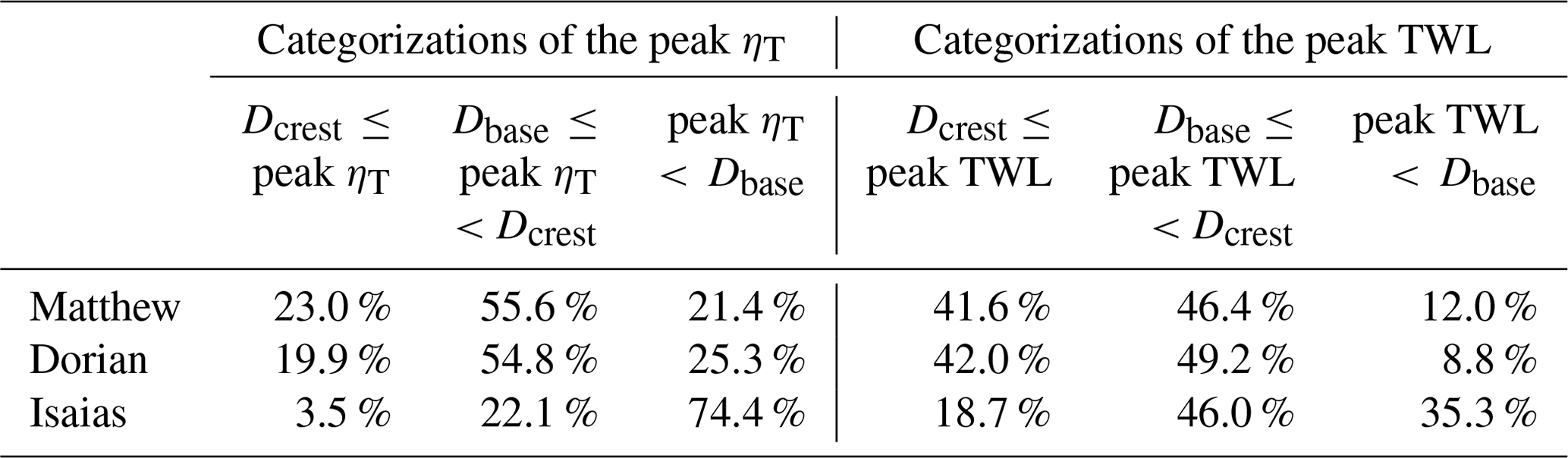
The proportion of coastal sites experiencing peak TWL ≥ D_crest was at least 1.8 times more than peak η_T ≥ D_crest (Table 2), which showed the importance of astronomic tides in coastal inundation levels. Matthew had a shorter distance to the coast along the SAB compared to Dorian, while Dorian had stronger intensity north of Georgia (Fig. 3 and Table 1). Consequently, Matthew and Dorian induced comparable peak η_T along the SAB.

In addition to the peak η_T, we used D_base as the threshold to compute the maximum continuous durations of η_T ≥ D_base (T_ETA; panels a1, b1, and c1 in Fig. 4) and TWL ≥D_base (T_TWL; panels a2, b2, and c2 in Fig. 4) along the SAB throughout each of the entire storm events. These were determined by calculating the maximum continuous duration that η_T or TWL was higher than the thresholds without interruption. D_base was applied here because less than 23 % of all coastal sites experienced peak η_T ≥ D_crest during the three TCs (Table 2). The averaged T_ETA along the SAB during Dorian (55.1 h) was longer than those during Matthew (32.5 h) and Isaias (7.1 h) (Fig. 4). Considering the contributions from astronomic tides, the averaged T_TWL values along the SAB were 27.5, 32.9, and 6.7 h during Matthew, Dorian, and Isaias, respectively (Fig. 4). Note that the difference in averaged T_TWL during Matthew and Dorian (i.e., 32.9–27.5 = 5.4 h) was 76 % smaller than the corresponding difference in averaged T_ETA (i.e., 55.1–32.5 = 22.6 h). This was mainly related to the smaller tidal range during Hurricane Matthew compared to Dorian. Although TWL was larger than η_T at high tides (crests of astronomic tidal signal), it was smaller than η_T at low tides (troughs of astronomic tidal signal). This pointed out the importance of the instantaneous tidal range in the inundation duration under extreme weather conditions.

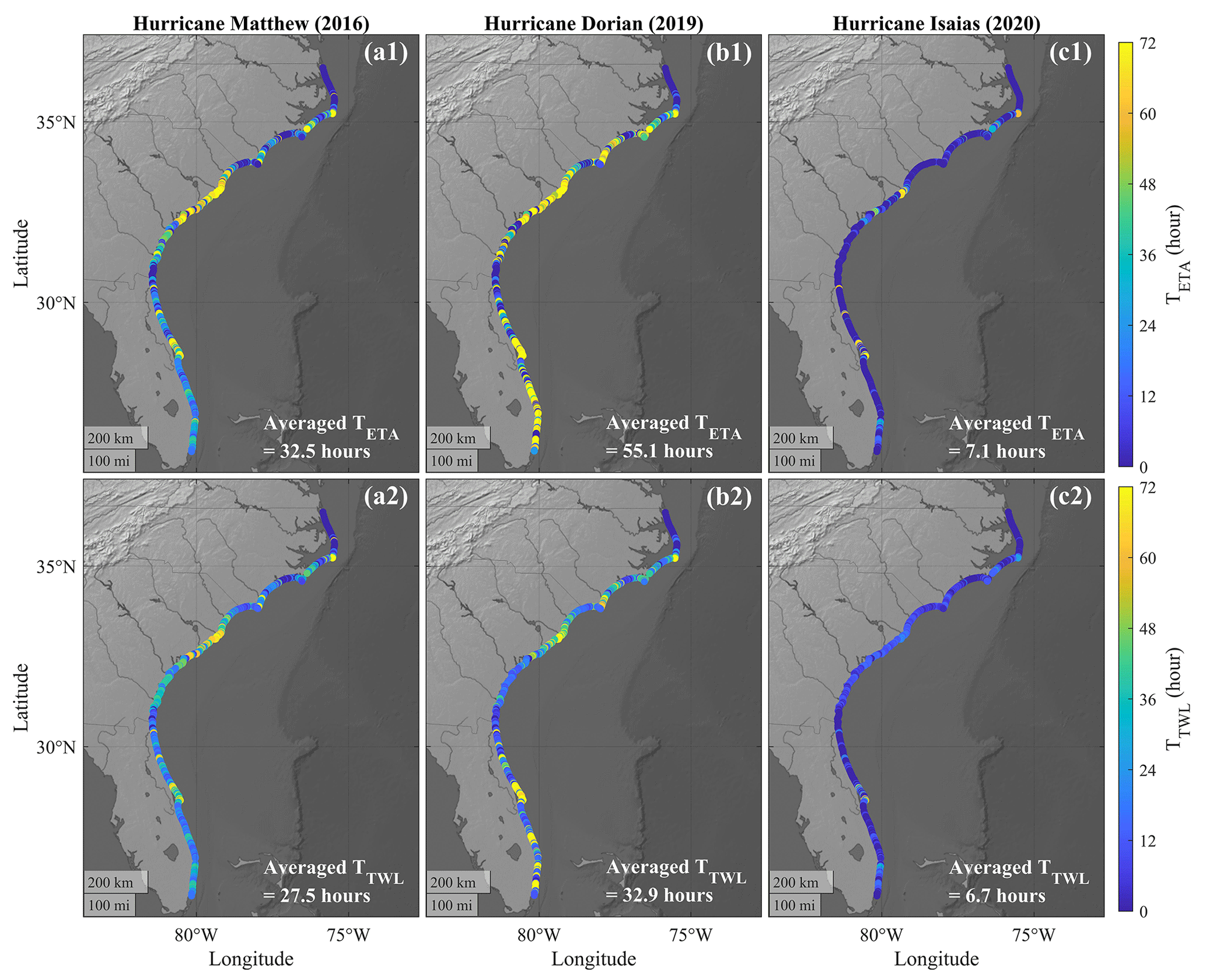
Figure 4 The maximum continuous duration of η_T (T_ETA; panels a1, b1, and c1) and TWL (T_TWL; panels a2, b2, and c2) over D_base at each USGS coastal site along the SAB throughout each of the three historical hurricanes.

We calculated the maximum continuous duration of $d/R_{\max }$ (i.e., normalized distance) ≤ 8.0 at each coastal site throughout each of the three storm events, where d was the distance between the TC eye and each coastal site along the SAB, and R_max was the instantaneous radius of maximum wind (Fig. 5). This threshold followed the distance threshold of near-TC field (Collins et al., 2018; Young, 2006). While Young (2006) also considered V_max in the definition of near-TC field, we did not consider the threshold for V_max here because V_max was relatively small along the SAB during Isaias. We found the duration of $d/R_{\max }\le$ 8.0 had a correlation coefficient (C_CORR)= 0.47 with T_ETA considering the coastal sites along the SAB during hurricanes Matthew, Dorian, and Isaias. In particular, the durations of $d/R_{\max }\le$ 8.0 during Matthew and Dorian (Fig. 5) showed similar patterns to T_ETA (panels a1, b1, and c1 in Fig. 4). Meanwhile, the path of Hurricane Isaias had short distances to Florida's southeast coast and resulted in the duration of $d/R_{\max }\le$ 8.0 longer than 48 h. However, it did not lead to longer T_ETA, primarily because of the weaker V_max of Isaias along the SAB.

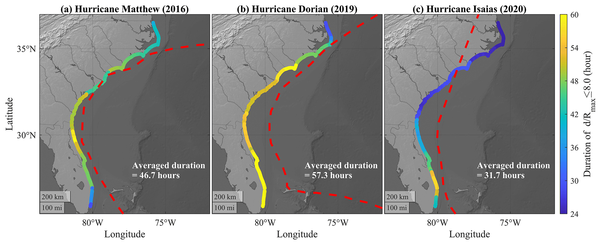
Figure 5 The durations of $d/R_{\max }\le$ 8.0 along the SAB during the three historical hurricanes. The dashed red curves represent the tracks obtained from the IBTrACS database of each hurricane.

4.3 Relative contributions of η_S and R₂ to η_T

In addition to the peak η_T along the SAB during the three historical hurricanes, we compared the proportions of η_S, wave setup, and wave swash at three specified locations: Edisto Island, South Carolina (32.51^∘ N, 80.26^∘ W); Sea Island, Georgia (31.20^∘ N, 81.33^∘ W); and the barrier island south of Matanzas Inlet, Florida (29.68^∘ N, 81.22^∘ W) (Fig. 6). Edisto Island, South Carolina (D_crest= 2.10 m and D_base= 1.26 m), and Sea Island, Georgia (D_crest= 3.49 m and D_base= 2.41 m), had relatively low dune elevations, in which dune overwash was more likely to occur during extreme weather events, according to the USGS (https://www.usgs.gov/news/national-news-release/fl-ga-sc-beaches-face-80-95-percent-chance-erosion-hurricane-matthew, last access: 31 March 2023). The peak η_T values south of Matanzas Inlet, Florida, during the storms were 1.41 to 1.62 m (51 % to 64 %) greater than the two other barrier islands mentioned above in the near-TC field during Matthew and Dorian (time instants shown by the vertical dashed yellow lines in Fig. 6). One of the factors causing higher estimated R₂ was the larger mean beach slope (β_m) at the barrier island south of Matanzas Inlet (0.151) compared to Sea Island (0.038) and Edisto Island (0.048) (Fig. A3). R₂ consisted of wave setup and wave swash. The percentage of wave swash in the peak η_T outnumbered that of wave setup by 25 % to 34 % at Sea Island and Edisto Island during all three TCs, while the wave swash only outnumbered wave setup by less than 9 % at the barrier island south of Matanzas Inlet (Fig. A4). Meanwhile, we found that η_S contributed less than 40 % in the peak η_T at the three locations as these three historical TCs approached. Surge levels at the peak η_T generally decreased from south to north during the three hurricanes, whereas wave setup and wave swash did not experience such a pattern.

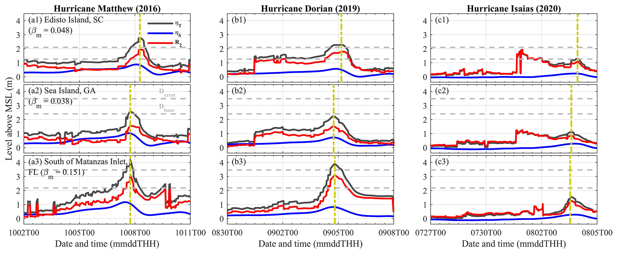
Figure 6 The time series of η_T (black curves), η_S (blue curves), and R₂ (red curves) at three selected locations during the three historical hurricanes. The horizontal dashed gray lines are the local D_crest and D_base measured by USGS before Matthew (2016), and the vertical dashed yellow lines are the peak η_T in the near-TC field.

Within the near-TC field, waves in most frequency bands kept receiving energy from the local wind, and η_T was directly impacted by the instantaneous TC characteristics. The peak η_T occurred within the near-TC field between 15:00 UTC on 7 October 2016 and 07:00 UTC on 8 October 2016 during Matthew, while it took place between 14:00 UTC on 4 September 2019 and 04:00 UTC on 5 September 2019 during Dorian (panels a1, a2, a3, b1, b2, and b3 in Fig. 6). The peak η_T at the three locations occurred in the near-TC field during Matthew and Dorian, without a second comparable peak η_T throughout the time series. The conditions during Isaias were unique and different from Matthew and Dorian. First, the instantaneous V_max did not reach 33 m s⁻¹ during Isaias when $d/R_{\max }\le$ 8.0 at most coastal sites along the SAB. Second, η_T generally experienced an abrupt increase before Isaias reached the coastal sites along the SAB. This earlier increase in η_T at Edisto Island (South Carolina) even exceeded the peak value within the near-TC field (panel c1 in Fig. 6). This increased η_T before the peak of the storm occurred between 21:00 and 23:00 UTC on 31 July 2020 at Sea Island and Edisto Island, when Isaias was still far away from these three selected locations (i.e., with distances larger than 1300 km).

η_S and R₂ at the coast depended on the instantaneous TC characteristics within the near-TC field. The differences between the peak η_T within the near-TC field during hurricanes Matthew and Dorian were less than 1.0 m at the three selected locations. The peak η_T at the same locations during Hurricane Isaias within the near-TC field (3 August 2022) was 1.0 to 2.7 m less than that of Matthew and Dorian. The η_S at the peak η_T during Isaias was 50 % to 80 % lower than that of Matthew and Dorian within the near-TC field at the three locations (numbers listed in Fig. A4). R₂ (i.e., the sum of setup and swash) at the peak η_T during Isaias was 40 % to 60 % smaller compared to that of Matthew and Dorian in the near-TC field. This was related to Isaias's smaller V_max within the SAB (28 % to 36 % smaller than Matthew and Dorian; Table 1).

Table 3 Maximum continuous durations of η_T and TWL over the local D_base at the three barrier islands during the three historical TCs in hours. T_ETA was the maximum continuous duration of the η_T ≥ D_base scenario; T_TWL was the maximum continuous duration of the TWL ≥ D_base scenario.

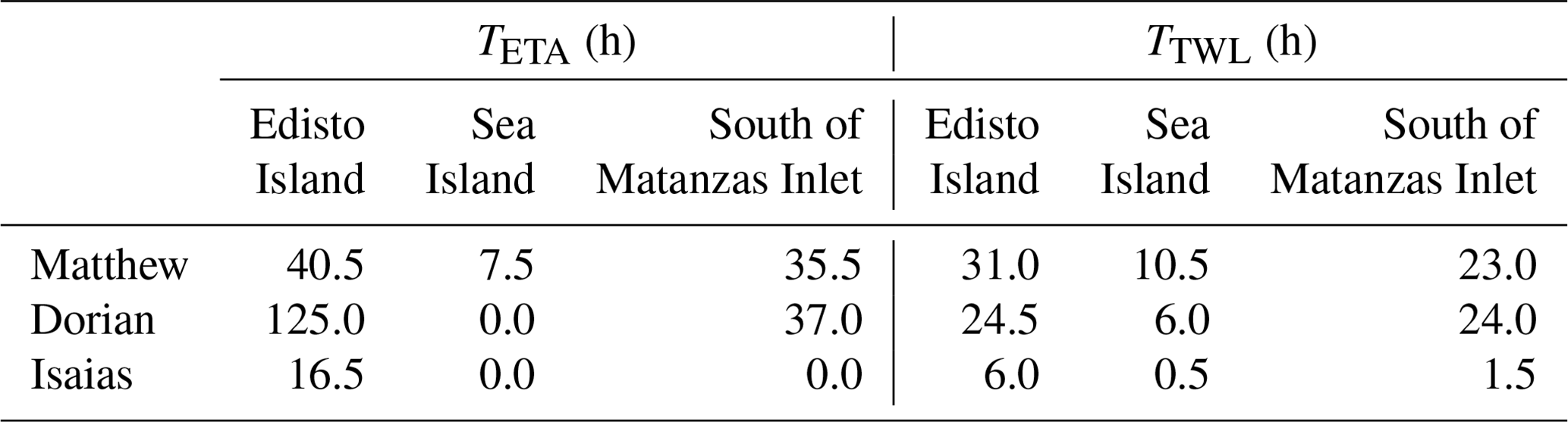
The duration of the same η_T category (η_T ≥ D_crest, D_base ≤ η_T < D_crest, and η_T < D_base) varied with TC characteristics. T_ETA at Edisto Island lasted up to more than 5 d during Dorian, which was much longer compared to T_ETA during Matthew and Isaias (40.5 and 16.5 h, respectively; Table 3). T_ETA at the barrier island south of Matanzas Inlet during Dorian (37.0 h) was longer compared to Matthew (35.5 h), but the difference was smaller than that at Edisto Island. While T_ETA primarily depends on TC characteristics, T_TWL also depends on the instantaneous local tidal range. The TWLs at tidal troughs were lower with a larger tidal range. This led to a shorter T_TWL when compared to T_ETA in the three hurricanes, as TWLs dropped lower than D_base at tidal troughs. Although Dorian had a stronger V_max and slower V_t along the SAB on average, Matthew and Isaias had shorter distances to the coast. Moreover, the tidal range during Matthew was approximately 40 cm smaller compared to Dorian and Isaias on average at the eight NOAA tide gauges (shown in Fig. 1). With similar V_max, shorter distances to the coast, and a smaller tidal range, Matthew had longer T_TWL at Edisto Island and Sea Island compared to Dorian (Table 3).

4.4 Storm-forced water level variation

Suh and Lee (2018) utilized two historical TCs to analyze and compare the propagation processes of forerunner surges and primary surges in the Yellow Sea, and these processes were linked to the heading direction, path, and translation speed of the storm. Similarly, we observed distinct patterns of storm-dependent water level component variations during three different storm events and at various locations along the SAB.

During Matthew and Dorian, the peak η_T occurred when the coastal sites started to be covered by the near-TC field, which was induced by the wind waves and η_S associated with higher TC intensities (i.e., larger pressure deficits and higher wind speeds). However, η_T at the three coastal sites had another local maximum at 15:30 UTC on 31 July 2020 during Isaias, when the storm was still located around 21.5^∘ N and 73.5^∘ W, i.e., south of the SAB (Fig. 7b and d). This was primarily the result of two factors. First, before entering the SAB (i.e., south of 26.0^∘ N and east of 79.0^∘ W), the translation speeds of Matthew (maximum of 7.52 m s⁻¹ and average of 4.17 m s⁻¹) and Dorian (maximum of 7.35 m s⁻¹ and average of 5.35 m s⁻¹) were slower compared to Isaias (maximum of 9.81 m s⁻¹ and average of 6.74 m s⁻¹). Xu et al. (2007) found that the swell energy and wavelength increased when V_t was comparable to the group wave celerity and under 13 m s⁻¹. This allowed wind waves to experience an extended wind fetch and resulted in the growth of wavelength and wave height. According to Eq. (1) (Stockdon et al., 2006), R₂ increases with the deep-water peak wavelength and the deep-water zero-order moment wave height. Second, before arriving at the Island of Hispaniola (19.0^∘ N), the swell generated by Matthew on its righthand side was blocked by the Island of Hispaniola and was unable to propagate towards the SAB on its path. By contrast, the swell generated by Isaias on its front-right quadrant was not blocked by any island (see Fig. 1). Thus, the condition during Isaias was better for the swell's wavelength to be lengthened and to propagate ahead of the storm.

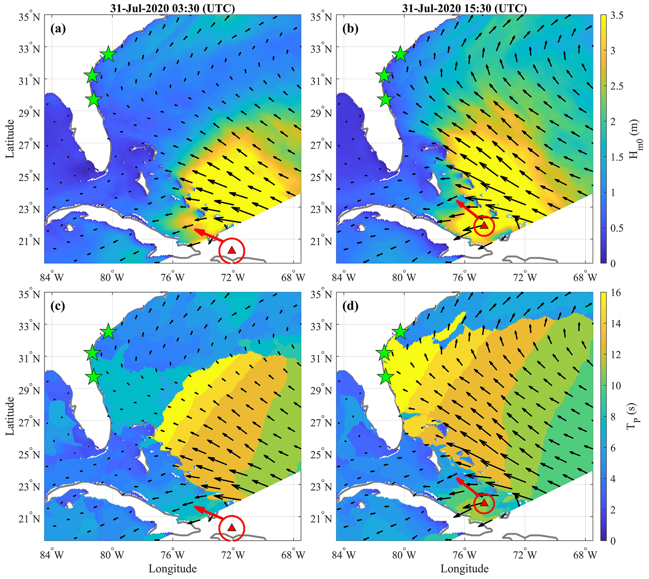
Figure 7 The propagation of the swells generated by Hurricane Isaias on its righthand side. The green stars indicate the three selected barrier islands, i.e., Edisto Island, Sea Island, and the barrier island south of Matanzas Inlet (from north to south). The red triangles represent the eye of Isaias, with the red circle denoting the instantaneous radius of maximum wind and the red arrow denoting the heading direction. The black arrows are the mean wave directions from the COAWST simulation. The color maps in panels (a) and (b) show the distribution of H_m0 at 03:30 UTC on 31 July 2020 and 15:30 UTC on 31 July 2020, respectively. The color maps in panels (c) and (d) show the distribution of T_P at 03:30 UTC on 31 July 2020 and 15:30 UTC on 31 July 2020, respectively.

According to the model results and linear wave dispersion relation, the peak wave period was 19.1 s, and the corresponding deep-water phase celerity was larger than 25 m s⁻¹ at Sea Island, Georgia, at 15:30 UTC on 31 July 2020 during Isaias (when the abruptly elevated R₂ occurred). This swell with a relatively long wave period generated by Isaias on its righthand side arrived at the SAB coast much earlier (1 to 2 d) than the storm, which led to an abrupt increase in R₂. Around 16:00 UTC on 1 August 2020, the instantaneous V_t of Isaias decreased from 7.0 m s⁻¹ to less than 4.5 m s⁻¹. Additionally, waves with different periods travel with different phase celerities according to linear wave dispersion relation. This is also consistent with the distribution pattern of peak wave periods shown in Fig. 7c and d (i.e., waves with higher T_P moved forward faster and approached the SAB earlier). Consequently, the wavelength of the swell arriving later at the SAB decreased, which led to a decrease in R₂.

4.5 Coastal impact regimes of Sallenger (2000) and the temporal variation in β_m

The dune elevations measured by USGS before Matthew did not reflect the realistic conditions during Dorian and Isaias, since the beach morphology (e.g., dune heights and beach slopes) changed in time. However, the time-invariant dune elevations allowed the present work to focus on determining the relative contributions of TC-induced water level components (η_S and R₂) during various TCs. The coastal impact regimes (Sallenger, 2000) were determined with the relative TWLs depending on storm-forced parameters (η_S and R₂), astronomic tides, and coastal morphology (dune elevations and beach slopes). However, the real coastal impact regimes during specific events require an update of the beach slopes and dune elevations. The problem was that this information was not always available at the spatial scale of this study.

To determine the sensitivity of the wave runup to the beach slopes, we used the post-Matthew β_m from Georgia to North Carolina measured by USGS (Doran et al., 2017) to compare TWLs and T_TWL associated with the model results of Hurricane Dorian with the pre-Matthew surveyed β_m (Fig. 8). We used the post-Matthew beach morphological information to determine the difference in the estimated storm-induced water levels. The post-Matthew dataset showed that β_m experienced an averaged decrease of −0.026 after Hurricane Matthew. According to Eqs. (1) and (2), TWLs and T_TWL during Hurricane Dorian would decrease considering the change in β_m. Results showed that 50 % of the coastal sites between Georgia and North Carolina experienced an absolute difference in simulated peak TWL of less than 0.5 m as β_m changed. The averaged decrease in peak TWL was 0.56 m with a standard deviation of 0.87 m. Meanwhile, an averaged decrease in T_TWL of 11.23 h was observed (Fig. 8).

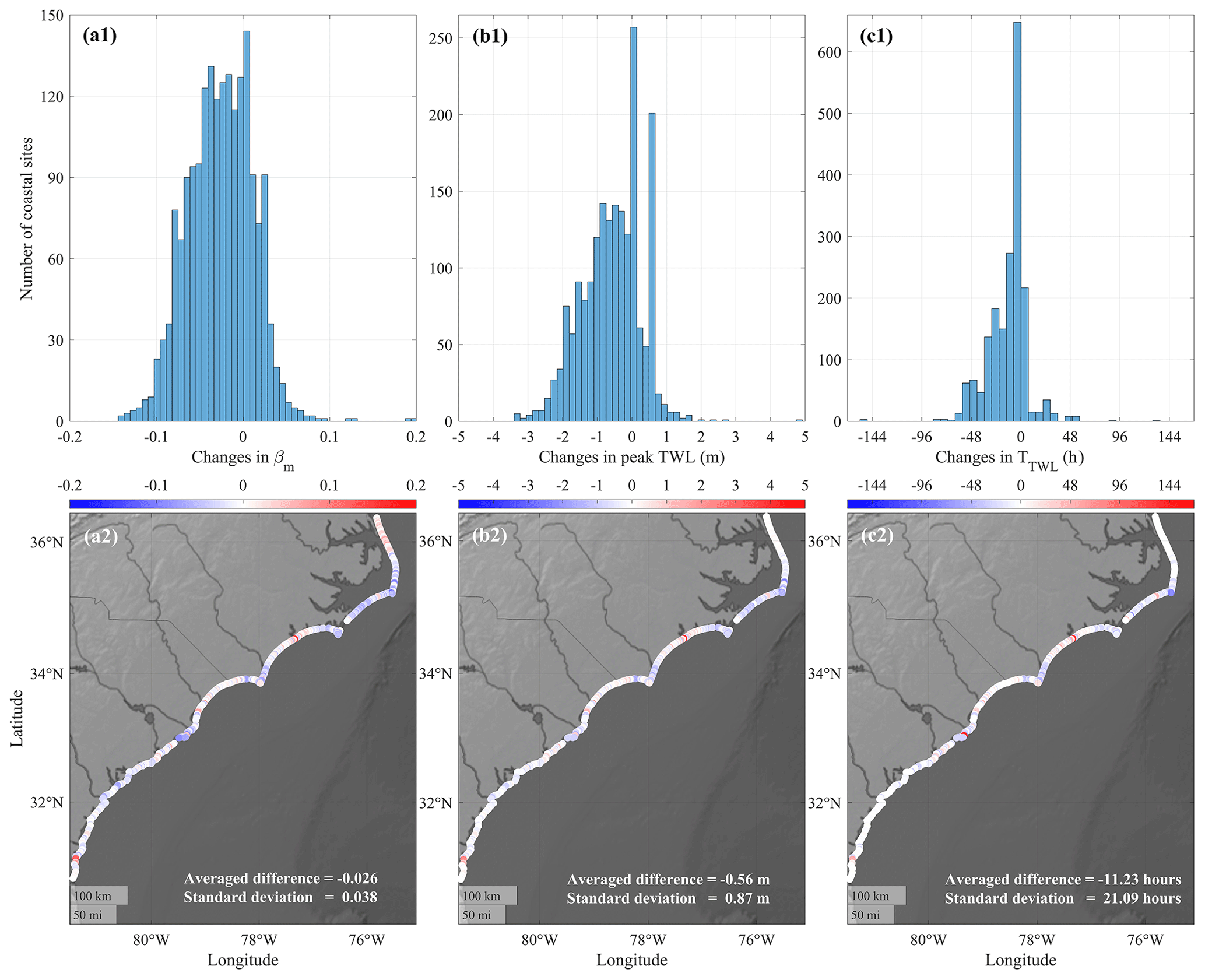
Figure 8 Histograms (a1, b1, c1) and spatial distributions (a2, b2, c2) of the differences in β_m, peak TWL, and T_TWL under pre- and post-Matthew conditions from Georgia to North Carolina coasts: (a1, a2) β_m, (b1, b2) peak TWL, (c1, c2) T_TWL.

Based on Sallenger's (2000) categorizations, our model results showed that at least 64.7 % of the peak TWLs (i.e., the sum of η_T and astronomic tides; Table 2) belonged to the overwash and inundation regimes during the three hurricanes under the assumption of constant dune elevations and β_m. However, dune heights and β_m are expected to decrease after storm events, which is consistent with the post-Matthew conditions from the observed data. While a decreased dune elevation led to more severe and longer impact regimes, a milder β_m resulted in a lower wave runup.

4.6 Arrival timing of the peak storm-dependent components

Beside beach morphology and TC-dependent parameters (${\mathit{\eta }}_{\mathrm{T}}={\mathit{\eta }}_{\mathrm{S}}+R_{\mathrm{2}}$), TC-independent parameters like astronomic tides also influenced the coastal impact regimes. In some cases, the peak TWL exceeded D_crest, while the peak η_T did not exceed D_crest. This was related to the coincidence of the timing of the high tide and the peak η_T. In the case that the peak η_T occurred at low tide, the peak TWL would be lower than the peak η_T. With the time-invariant dune elevation, both the peak TWL and the peak η_T did not reach D_crest at this location during Dorian. However, both peak TWL and peak η_T would exceed D_crest in the case that the dune elevation became lower.

4.7 Effects of TC properties on the durations of η_T

Hurricane Dorian traveled with a slow V_t (3.27 m s⁻¹) on average, which was not only slower than the other two historical storms but also slower than the global average of TCs in all categories (4.20 to 6.00 m s⁻¹). While the instantaneous V_max had significant impacts on η_T, the slow movement of the TC resulted in a longer duration of T_ETA at which a specific location was under its impact. The peak η_T did not reach D_base (T_ETA= 0.0 h) at Sea Island during Dorian, while the peak η_T at the same location exceeded D_base for 6.0 h during Matthew. V_t was the primary factor determining T_ETA at the other two coastal sites. However, as V_max increased and/or the distance to the TC eye decreased, T_ETA might also increase. The variations in T_ETA at the three coastal sites during the three historical TCs implied that the peak water level alone may not be sufficient to predict the coastal impacts in practical scenarios. For instance, T_ETA experienced a 67.7 % difference (i.e., 84.5 h difference) at Edisto Island between Matthew and Dorian (Table 3), while the peak η_T at this location belonged to the same categories during these two TCs.

4.8 Estimations of R₂ using different empirical formulas for R₂

Stockdon et al. (2006) used different formulas of R₂ for the 0.3 ≤ξ₀ < 4.0 and ξ₀ < 0.3 scenarios (Eqs. 1 and 2). The range 0.3 ≤ξ₀ < 4.0 represents intermediate to more reflective beach scenarios. The formula of Senechal et al. (2011) was proposed based on the regression of their observed runup data to improve the estimation under highly dissipative and saturated beach conditions (ξ₀ < 0.3) specifically (Eq. 4).

We compared the R₂ estimated by the formulas of Stockdon et al. (2006) and Senechal et al. (2011) at the same locations previously considered (Edisto Island, South Carolina; Sea Island, Georgia; and the barrier island south of Matanzas Inlet, Florida) during the three historical hurricanes (Fig. 9). The difference between the peak R₂ estimated by the two formulas reached up to 1.34 m at the barrier island south of Matanzas Inlet (panels a3 and b3 in Fig. 9; Stockdon's prediction was 76 % higher than Senechal's prediction during Matthew and Dorian).

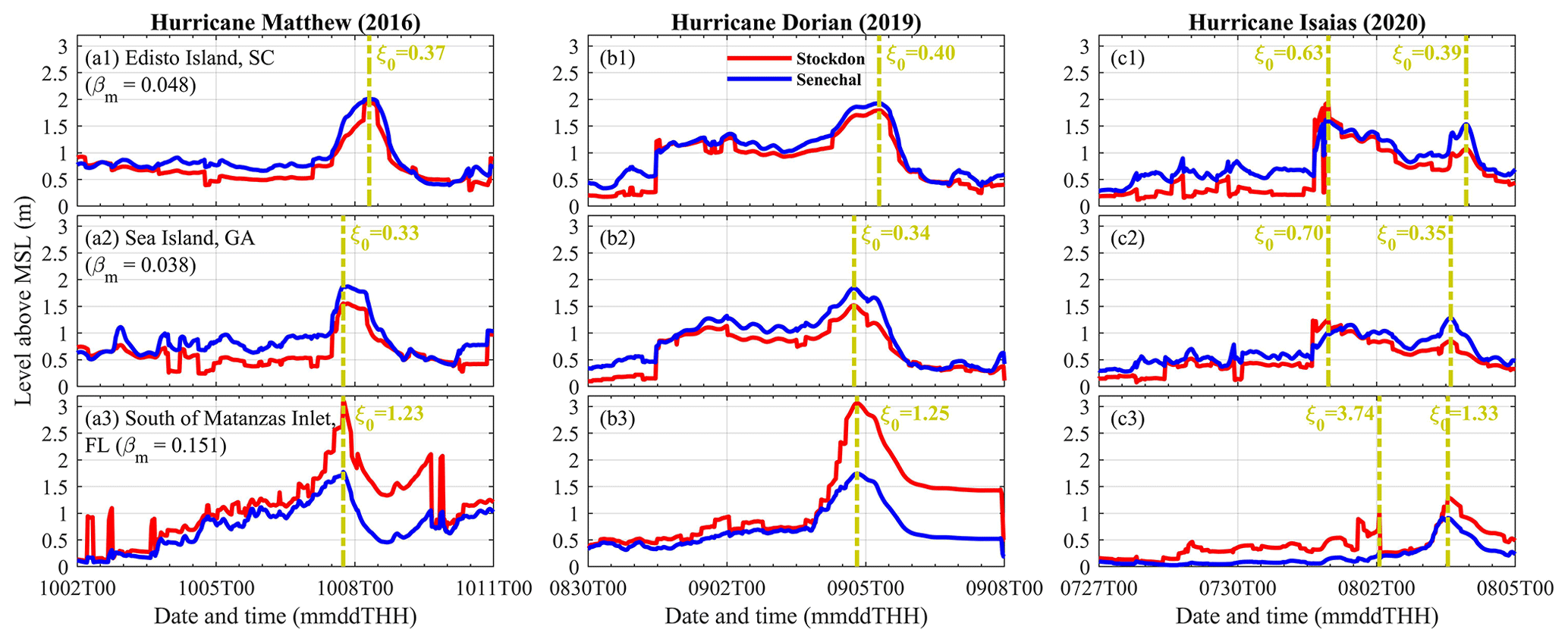
Figure 9 The R₂ estimated by the formulas of Stockdon et al. (2006; red curves) and Senechal et al. (2011; blue curves) at the three coastal sites during the three hurricanes. The Iribarren numbers (ξ₀) corresponding to the peak R₂ (vertical dashed yellow lines) are listed.

The R₂ estimated by Stockdon's formula showed a distinctive pattern during Isaias: another peak occurred before the storm approached the observed location. This was related to Isaias's unique path and faster V_t. The R₂ estimated by Senechal's formula did not show this pattern, since Senechal et al. (2011) did not include the effect of L₀. The results showed that Stockdon's approach returned a larger R₂ compared to Senechal et al. (2011), especially under ξ₀ > 0.6 (with a difference of up to 1.34 m). On the contrary, Senechal et al. (2011) gave larger values of R₂ under ξ₀ < 0.5 compared to the results by Stockdon et al. (2006) but with a smaller difference (i.e., less than 0.50 m).

We computed the differences between the time series of R₂ derived from the formulas of Stockdon et al. (2006) and Senechal et al. (2011) (i.e., ${\mathit{\delta }}_R=R_{\text{2-Stockdon}}-R_{\text{2-Senechal}}$) along the SAB. Next, we calculated the correlation coefficients (C_CORR) between δ_R and five parameters: ξ₀, H₀, L₀, T_P, and β_m. It was found that β_m, ξ₀, and L₀ had higher C_CORR, which were 0.64, 0.47, and 0.42, respectively. δ_R increased as the mean beach slope, the Iribarren number, and the deep-water peak wavelength increased, which resulted in more reflective beach conditions. Stockdon's approach predicted that R₂ increased as wavelength increased under certain conditions (faster V_t and TC path allowing the swell to propagate toward the coasts).

5 Conclusions

We used the coupled ROMS–SWAN modeling system to simulate η_S and the wave fields (wave energy spectrum and bulk wave parameters) within the SAB during Matthew (2016), Dorian (2019), and Isaias (2020). Following Serafin and Ruggiero (2014), we used the measured η₀ and waves to estimate the TWLs from observations. We used linear wave theory to calculate the deep-water wave parameters and estimate the 2 % exceedance wave runup using Stockdon's (2006) empirical formula. We followed the same procedure with the results from COAWST and compared the TWLs estimated with both methods. The COAWST model results showed good agreement with the peak TWLs, peak storm surges, peak wave runups, and exceedance durations.

We used our model results to compare the peak η_T along the SAB and at three coastal sites specifically. The instantaneous V_max and the distance to the hurricane eye were the key factors determining the peak η_T within the near-TC field, whereas the maximum continuous duration of η_T and TWLs over given thresholds were primarily determined by V_t and the distance to the hurricane eye. The contributions of wave runup (i.e., the sum of wave setup (16 % to 38 %) and wave swash (41 % to 57 %)) to the peak η_T were usually higher than η_S (17 % to 40 %) at the three selected coastal sites during the three historical TCs. The variability in η_S (up to 75 %) at the peak η_T under different TC properties was larger than that of the wave runup (i.e., the sum of wave setup and wave swash; less than 59 %). These wave-dependent parameters were not only functions of the TC characteristics but strongly depended on the local coastal morphology (e.g., beach slope). The time series of η_T revealed that with specific TC characteristics (e.g., path, heading direction, and V_t), the peak η_T might occur before the storm's peak (i.e., outside the near-TC field). This was observed in the case of Hurricane Isaias as the hurricane traveled with a fast instantaneous V_t (maximum of 9.81 m s⁻¹ and average of 6.74 m s⁻¹, which was 1.1 to 2.3 times the global average in all categories) 2 to 3 d before approaching the location.

Two empirical formulas of wave runup estimation were compared. Stockdon's formula predicted the extreme prestorm swells associated with the TC's faster translation speeds, whereas this peak was not observed when using Senechal's empirical formula. Since runup observations during these storms were unavailable, it was not possible to determine which empirical formula was giving the best predictions. Given the relevance of accurately estimating TWLs, more observations of the wave runup during TCs are needed for the verification and calibration of wave runup parameterizations. With the present analysis of historical storms, it was difficult to determine the individual effect of each TC characteristic on TWLs. Further numerical experiments and analysis employing synthetic and idealized TCs are needed to quantify the individual impacts of V_t, V_max, distance to the coast, and beach slope on TWLs and, thus, the coastal morphological impacts.

Appendix A

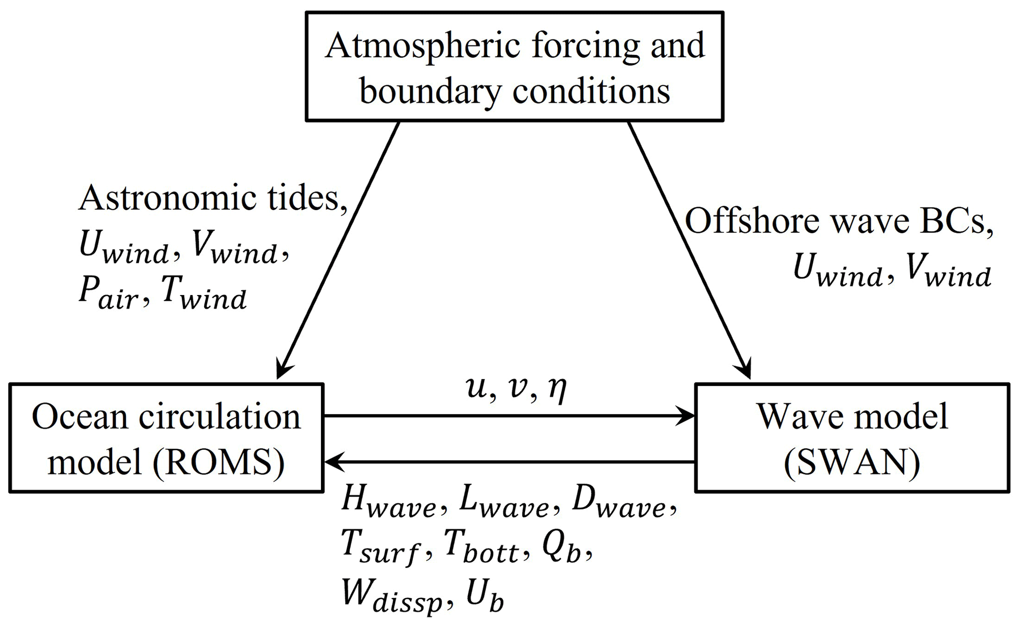
Figure A1 Computational flowchart of ocean circulation–wave coupling using the COAWST modeling system.

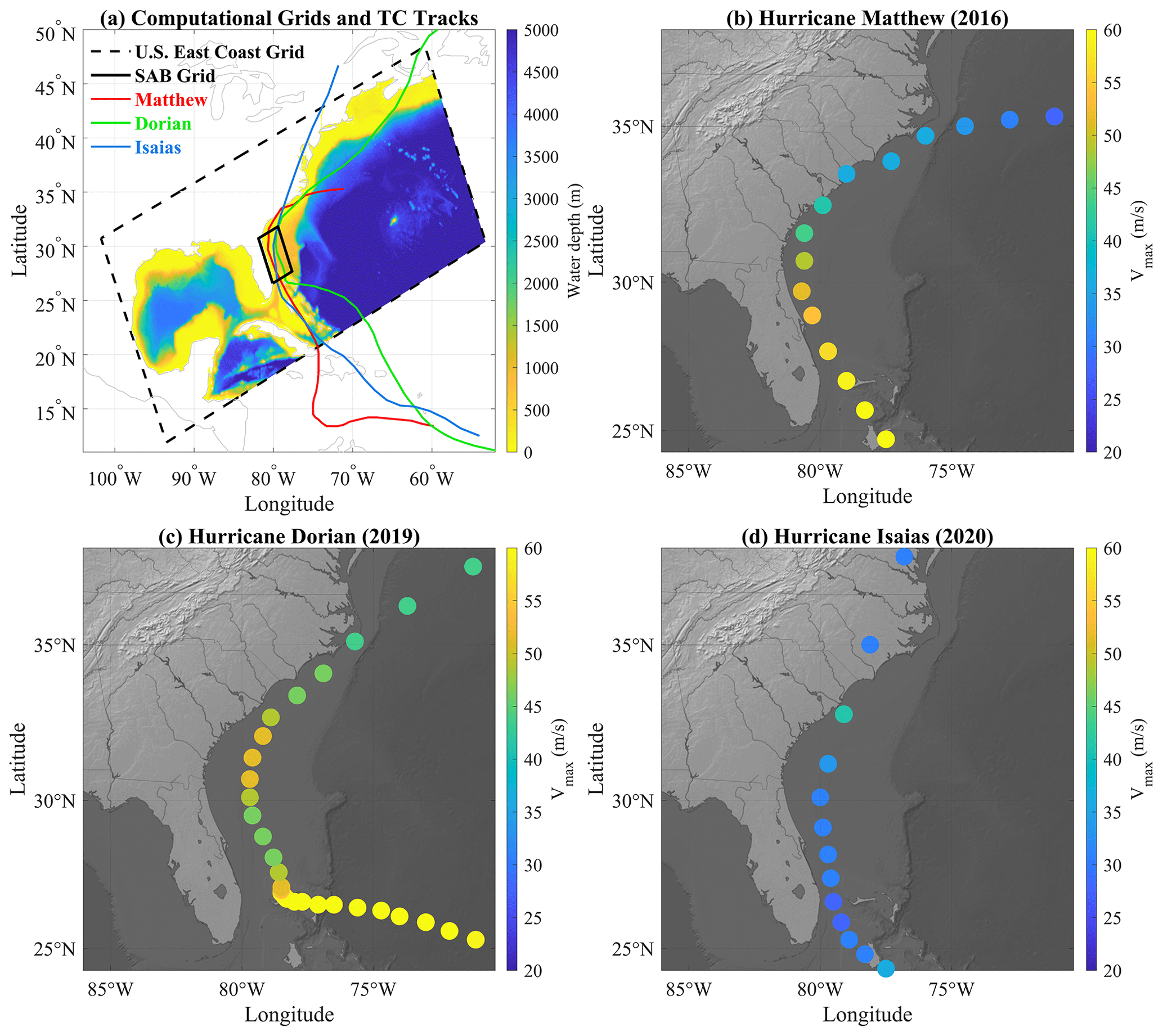
Figure A2 (a) International Best Track Archive for Climate Stewardship (IBTrACS) data of the three TCs as well as computational domain and bathymetry (red: Matthew, green: Dorian, blue: Isaias, black: the boundaries of computational grids, hypsometric map: water depth). Panels (b), (c), and (d) illustrate the tracks of the TCs (position of the dots), with the color map of the circles representing the maximum sustained wind during hurricanes Matthew, Dorian, and Isaias, respectively. The time interval between adjacent dots was 6 h.

Figure A3 Pre-Matthew mean beach slopes along the SAB measured by USGS.

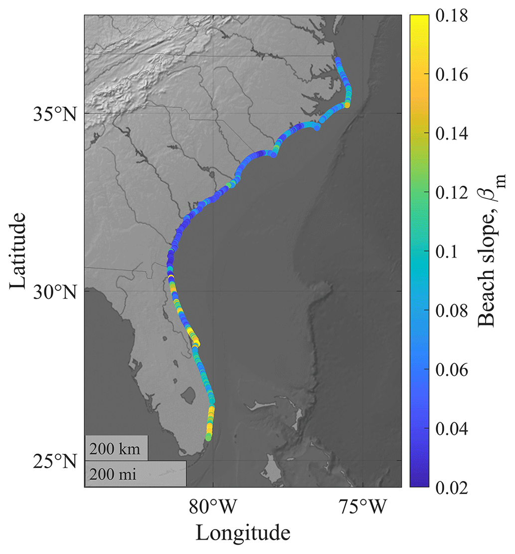
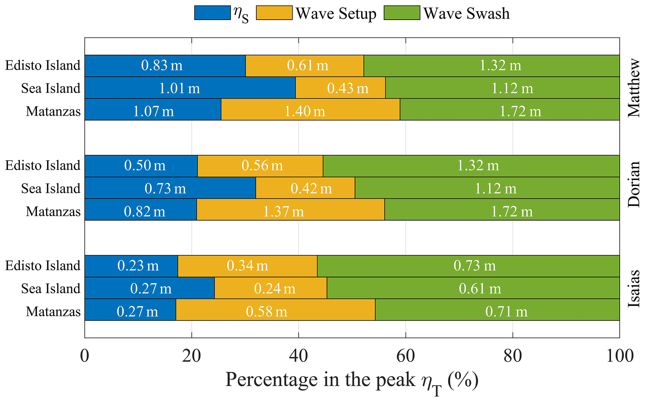
Figure A4 The contributions of η_S, wave setup, and wave swash in the peak η_T during the three historical hurricanes at the three coastal sites: south of Matanzas Inlet, Florida; Sea Island, Georgia; and Edisto Island, South Carolina, with the corresponding contribution of each component (%) in the peak η_T and the level listed by the number written in white font.