A new European coastal flood database for low–medium intensity events

Coastal flooding is recognized as one of the most devastating natural disasters, resulting in significant economic losses. Therefore, hazard assessment is crucial to support preparedness and response to such disasters. Toward this, flood map databases and catalogues are essential for the analysis of flood scenarios, and furthermore they can be integrated into disaster risk reduction studies. In this study and in the context of the European Coastal Flood Awareness System (ECFAS) project (GA 101004211), which aimed to propose the European Copernicus Coastal Flood Awareness System, a catalogue of flood maps was produced. The flood maps were generated from flood models developed with LISFLOOD-FP for defined coastal sectors along the entire European coastline. For each coastal sector, 15 synthetic scenarios were defined focusing on high-frequency events specific to the local area. These scenarios were constructed based on three distinct storm durations and five different total-water-level (TWL) peaks incorporating tide, mean sea level, surge and wave setup components. The flood model method was extensively validated against 12 test cases for which observed data were collated using satellite-derived flood maps and in situ flood markers. Half of the test cases represented well the flooding with hit scores higher than 80 %. The synthetic-scenario approach was assessed by comparing flood maps from real events and their closest identified scenarios, producing a good agreement and global skill scores higher than 70 %. Using the catalogue, flood scenarios across Europe were assessed, and the biggest flooding occurred in well-known low-lying areas. In addition, different sensitivities to the increase in the duration and TWL peak were noted. The storm duration impacts a few limited flood-prone areas such as the Dutch coast, for which the flooded area increases more than twice between 12 and 36 h storm scenarios. The influence of the TWL peak is more global, especially along the Mediterranean coast, for which the relative difference between a 2- and 20-year return period storm is around 80 %. Finally, at a European scale, the expansion of flood areas in relation to increases in TWL peaks demonstrated both positive and negative correlations with the presence of urban and wetland areas, respectively. This observation supports the concept of storm flood mitigation by wetlands.

1 Introduction

Flood hazard and risk are subjects of high concern due to the destruction and high cost caused by flooding. In the United States, 8 of the 10 most costly weather and climate disasters between 1980 and 2010 were floods, and extensive efforts have been made to assess flood hazard, gathering coastal, fluvial and pluvial risk for present and future climate scenarios (Bates et al., 2021). In Europe, between 1998 and 2009, flooding, mainly fluvial, was the most recorded natural disaster resulting in the largest overall economic losses (European Environment Agency, 2010). The role played by early warning systems (EWSs) is thus critical to support preparedness and response after such disasters. Since 2012, as part of the Copernicus Emergency Management Services, the European Flood Awareness System (EFAS) has become operational, predicting fluvial flood magnitude for the major rivers of the continent (Smith et al., 2016; Dottori et al., 2017). The daily streamflow forecast is connected to a database of flood hazard maps (Dottori et al., 2022) such that, using a rapid mapping process, event-based rapid risk assessments can be produced and provided to stakeholders and decision-makers. The advantages of such a system are multiple with, at local scale, a joint evaluation of fluvial risks and, at European scale, shared information for prioritizing and coordinating support across the national emergency services (Dottori et al., 2017).

No such EWS currently exists for coastal flooding at European scale, despite coastlines coming under growing pressure due to the increasing coastal population and infrastructure along with exposure to extreme events (Merkens et al., 2016; Calafat et al., 2022; Portner et al., 2022). It is in this context that the H2020 European Coastal Flood Awareness System (ECFAS) project (a proof of concept for the implementation of the European Copernicus Coastal Flood Awareness System, GA no. 101004211, https://www.ecfas.eu/, last access: 11 November 2023) aimed to suggest tools for European coastal risk EWSs. Similar to the EFAS system, the ECFAS concept relies on a forecast of coastal extreme water level (Irazoqui Apecechea et al., 2023) that is connected to a flood map catalogue, allowing for rapid flood risk assessment. Indeed, a catalogue gathers maps representing different possible flood scenarios affecting a coastal area that could be quickly retrieved without the necessity to run operational models. As these flood scenarios are defined by the nearshore forcing condition affecting the area, it is then assumed that every real flood scenario could be represented by the catalogue's equivalent with the forcing conditions that are the most similar to the real one. Coastal flood hazard assessment is usually performed at a local scale, and only a few studies targeted large and continent-wide scales (Barnard et al., 2014; Hinkel et al., 2014; Mokrech et al., 2015; Forzieri et al., 2016; Muis et al., 2016; Vousdoukas et al., 2016). Mokrech et al. (2015) built the Coastal Fluvial Flood (CFFlood) model from the global Dynamic Interactive Vulnerability Assessment (DIVA) database (Vafeidis et al., 2008) using coastal flood zones generated statically, such as with the bathtub method, for 1-, 10-, 100- and 1000-year events. Muis et al. (2016) built the GTSR model, also using a static method, to estimate the flood hazard for a 100-year extreme sea level scenario. Similar to the GTSR model, the TUD model was developed for the “Risk analysis of infrastructure networks in response to extreme weather” (RAIN) project, focusing on return levels of 10, 30, 100 and 200 years (Groenemeijer et al., 2016; Paprotny et al., 2016). It is only with the work of Vousdoukas et al. (2016) that a coastal flood hazard assessment was based on a flood dynamic model, hereafter referred to as the JRC model. They used 100 m resolution LISFLOOD-FP models (Bates and De Roo, 2000; Bates et al., 2010) to simulate the flood propagation for a 100-year return level scenario. The accuracy of the GTSR, JRC and TUD flood assessments was estimated at large scale by Paprotny et al. (2019) through comparisons with reference maps such as official national study maps, published research maps and an observed flood extent map. In their work, they highlighted a need for better analysis of the model's accuracy to be shared with stakeholders and concluded that there was a low performance by the statically generated databases, as also pointed out by Bates et al. (2005), Seenath et al. (2016), Vousdoukas et al. (2016), and Gallien et al. (2018).

In light of the above, there is a lack of European coastal flood hazard assessments using more accurate dynamic methods with a robust validation process. In addition, the existing databases focused on high-return-level events. However, low-return-level to frequent events could be of interest to the stakeholders in EWSs (Alves et al., 2022). In the frame of the ECFAS project, a new database of coastal flood maps was generated to assess the flood hazard at European scale for small–medium return events, hereafter referred to as the ECFAS flood map catalogue. While the previous flood databases rely on the characterization of the forcing based only on the water return levels, the present analysis additionally integrates the storm duration, as recommended by Wahl et al. (2011), leading to 15 storm scenarios forcing the models. The objectives of the present paper are twofold: first, to present the ECFAS flood catalogue alongside the methodology used to produce it, as well as the validation of the modeling method through the simulation of 12 test cases, the assessment of the catalogue capacity to represent real events and its limitations; second, to assess the flood hazard patterns and sensitivity to the different scenarios across Europe. To go further, and as an application of the catalogue use, connections between the flood sensitivities and land use and coverage data in Europe were investigated.

2 Datasets

2.1 Topography

The European digital elevation model (DEM) COP-DEM EEA-10, which is part of the Copernicus DEM products (European Space Agency and Airbus, 2022), was used as topography data. The horizontal spatial resolution is ∼10 m with an absolute vertical accuracy better than 4 m. The associated waterbody mask (European Space Agency and Airbus, 2022) was used to extract the coastal water extent and to identify the coastline. These data were used to build the model grid and the boundary condition positions of the flood model.

2.2 LU/LC data

The EEA (European Environment Agency) LU/LC (land use and land cover) Coastal Zone 2018 layer (CZ layer; European Environment Agency, 2020; Innerbichler et al., 2021), which is part of the Copernicus Land Monitoring Service, was used to define the friction parameter. The classification of the Copernicus CZ layer was derived from very high-resolution (VHR) satellite data and other available Earth observation data, leading to 71 classes of environments. The CZ layer was quality checked in the framework of the ECFAS project in order to produce a coastal dataset (Ieronymidi and Grigoriadis, 2022).

2.3 Total-water-level data

Total water levels (TWLs) at the coast include mean sea level, tides, atmospheric surges, wave setup and swash (Melet et al., 2018). In the present work, the TWLs were extracted from the 10-year ECFAS combined hindcast (Melet et al., 2021) covering the time window 2010–2019. This hindcast relied on a linear addition of the different components. The tide and mean sea level were selected from FES2014 (Lyard et al., 2021) and the Copernicus Marine high-resolution global ocean reanalysis GLORYS12 (Lellouche et al., 2021), respectively. The storm surge component was obtained using an upgraded version of the ANYEU-SSL ocean model (Fernández-Montblanc et al., 2020): the grid resolution was increased to 2.5 km at the coastline and the atmospheric forcing was upgraded to ERA 5 global reanalysis (Hersbach et al., 2020). The TWLs were validated by comparison against tide gauge data for both average and extreme events. Overall, the hindcast showed a good performance, with 90 % of RMSE values relative to the maximal observed water level being below 15 % for the entire period. Additionally, more than 80 % of the relative RMSE values are below 20 % during extreme events (Melet et al., 2021). For the ECFAS combined hindcast, the swash component was discarded and the wave setup η_wsu was approximated by the generic formulation derived by Holman and Sallenger (1985) and recommended by the US Army Corps of Engineers (2002):

$$\begin{array}{}\text{(1)}& {\mathit{\eta }}_{\mathrm{wsu}}=\mathrm{0.2}\times H_{\mathrm{s}},\end{array}$$

where H_s is the significant wave height. For the ECFAS hindcast, H_s values were taken from the Copernicus Marine Environment Monitoring Service (CMEMS) regional wave hindcast. Parameterizing the wave setup is common practice (Dodet et al., 2019), as an accurate representation of the nearshore wave components needs high-resolution wave models that are not always available, especially at the large scales targeted in this work. So this approximation is considered sufficient in the present work. When the TWL time series were not included into the ECFAS hindcast time window, such as during 2020, the relevant ocean and wave models from the CMEMS database were used (Clementi et al., 2021; Korres et al., 2021).

2.4 Test cases and observed data

In the present work, 12 test cases were identified across Europe from the storm database of Souto Ceccon et al. (2022) for validation purposes (Table 1 and Fig. 1).

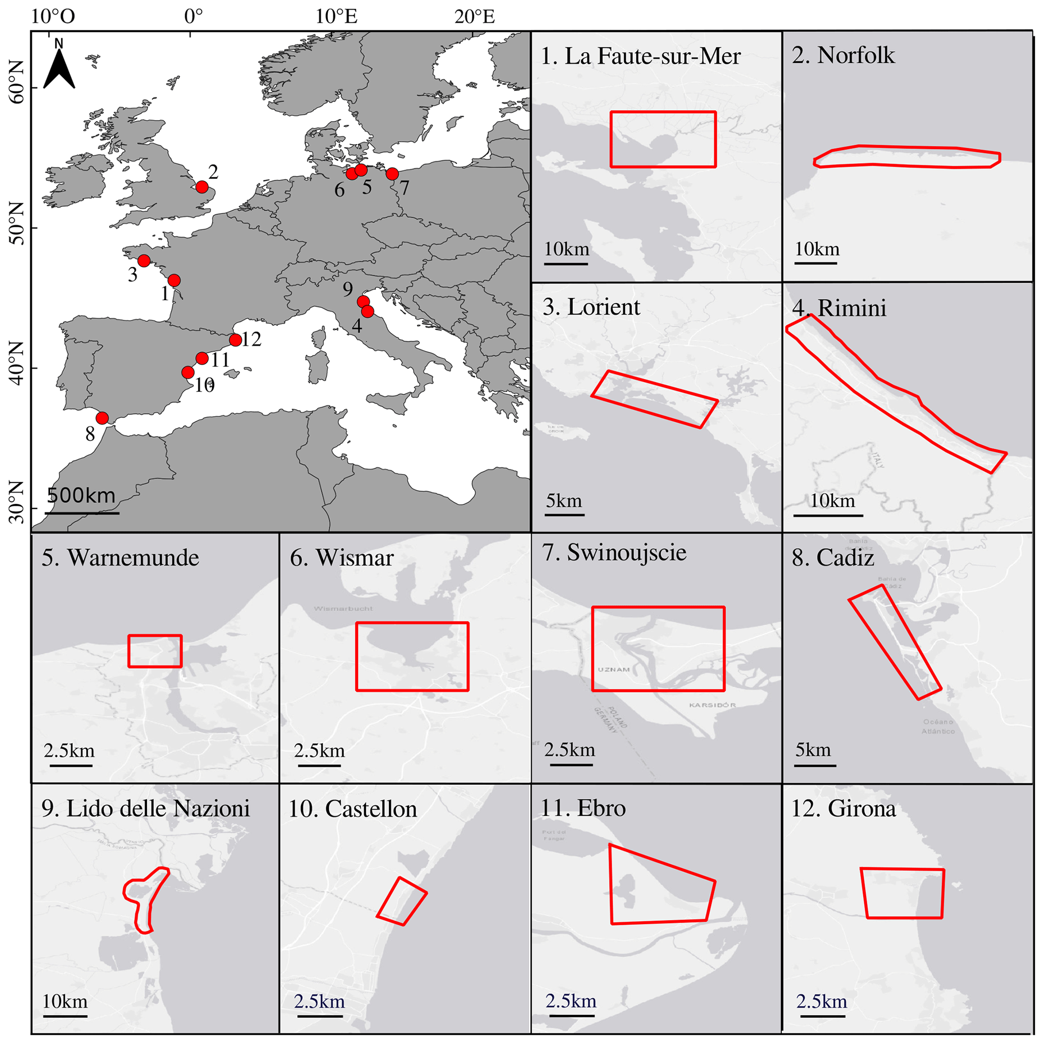
Figure 1 Location and area of interest of each test case extracted from the extreme event ECFAS database (Souto Ceccon et al., 2022) considered for the validation of the flood method. For details of the test cases, refer to Table 1.

Table 1 List of the test cases considered from the ECFAS extreme event database for the validation of the flood method and for which observed data were gathered. The acquisition delta time corresponds to the time lapse between the event and post-event image acquisition [d]. NA means sources and/or identifiable flood markers are not available.

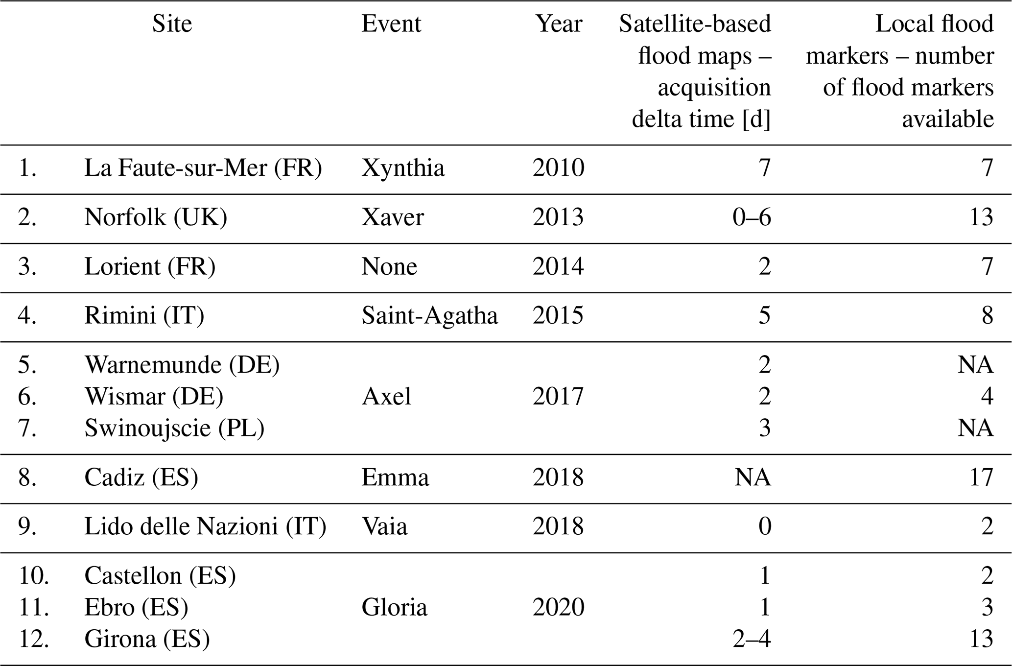
These test cases represent a large variety of coastal morphologies and oceanographic conditions (tidal range, storm surge level and wave energy) covering storms that occurred between 2010 and 2020 throughout Europe. This list gathers eight events covering 12 sites. Among the major events in the list, there are test cases covering the storm Xynthia (2010) that hit La Faute-sur-Mer (France), the storm Gloria (2020) that hit the Mediterranean Spanish coast and the storm Xaver (2013) that hit Norfolk (UK).

Two types of observed data were retrieved for the validation analysis: flood extension derived from satellite images and in situ observations.

2.4.1 Satellite-based flood map

Flood mapping of historical events is highly dependent on the availability and quality of archived satellite images. The most relevant acquisitions in terms of timing with regards to the event, type of image, resolution and acquisition conditions were selected to detect flooded areas. The satellite-derived flood extents were generated by differentiating the visible water surfaces between the pre-event image used as reference and the post-event image. Water surfaces were mostly extracted using an automated workflow and manually refined if needed. In the case of radar images, the discrimination between water and non-water surfaces relied on the backscatter coefficient value: water surfaces typically hold low backscattering values as they are usually smooth and flat, reflecting the radar pulse away from the spacecraft. In the case of optical images, water was extracted using the well-known Modified Normalized Difference Water Index (NDWI) (Xu, 2006) for images with a shortwave infrared band (Copernicus Sentinel-2, Landsat missions, SPOT 5). Other optical images, mainly VHR images, were analyzed using a manual approach. The satellite images are acquired in the aftermath of an event; the time lapse between their acquisition and the events considered in the test cases are indicated in Table 1.

2.4.2 In situ flood markers

The in situ flood markers were retrieved by analyzing the sources of information collected by Souto Ceccon et al. (2022), including, among others, videos, news and technical reports. Focusing on the areas of interest (Fig. 1), the flood markers were precisely geolocalized and described by reviewing those already identified by other reports or scientific papers or by thoroughly analyzing pictures and/or videos with visible flooding. The collected flood markers indicate flooded points or flood extension limits. In the present work, only flood markers that were precisely geolocated were used. The number of flood markers per test case is indicated in Table 1.

3 Methods

3.1 Flood modeling approach

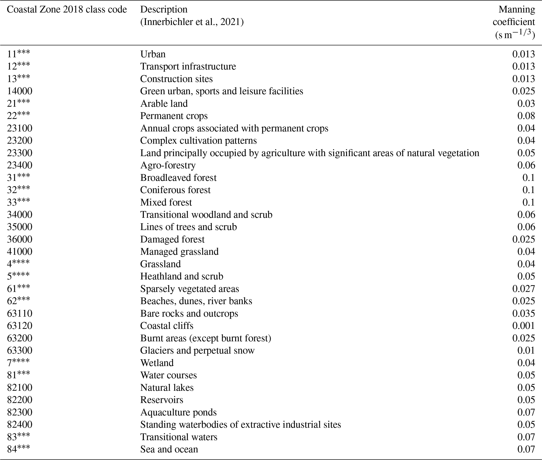
The flood modeling of this study was performed with the widely used LISFLOOD-FP model (Bates and De Roo, 2000). The acceleration solver was used as the numerical flood plain solver (Bates et al., 2010). It simplifies the shallow-water equations by neglecting the convective acceleration terms. This floodplain solver is usually recommended for coastal modeling and was shown to perform as well as solvers integrating the full shallow-water equations with the advantage of keeping the computational time reasonable (Bates et al., 2010; Neal et al., 2012; Shaw et al., 2021). A comparison between results from both 50 and 100 m grid resolutions and observed data was performed to evaluate the impact of the grid resolution on the flood maps (not shown). The 100 m models globally performed slightly better, probably due to the smoothing of local barriers and protection, thus generating larger hazard maps which could compensate for a slight underestimation of the forcing (see Melet et al., 2021). At the same time, the 50 m resolution drastically increased the computational time. In consequence, without quantifiable improvements from the finer models, a 100 m resolution was chosen to support a balance between quality and computational feasibility. Elevation data were interpolated from the DEM data, and spatially varying friction grids were derived from the LU/LC Coastal Zone 2018 layer by associating each class with a literature-based Manning coefficient (Chow, 1959; Papaioannou et al., 2018); the values used in this study are gathered in Table A1. This configuration was identical for all models and was supported by model configuration sensitivity. TWL time series were imposed as boundary conditions at the coastline of the flood model. The coastline was identified by the DEM data, and the TWLs were directly interpolated from ocean model data using a nearest-point method (see Sect. 3.3). The outputs of interest of the model are the maximum flooded area (M.F.A.) extension with the maximum water depth and velocity. They will be referred to hereafter as the flood maps.

3.2 Validation of the flood model

To assess the accuracy of the flood method and configuration applied to generate the ECFAS catalogue, flood models were developed for the 12 test cases (Sect. 2.4) using the real TWL time series to force the flood model. The TWL time series were extracted from the ECFAS hindcast (as detailed in Sect. 2.3) with the exception of the test cases covering the storm Gloria (2020, not included in the ECFAS hindcast) for which they were taken from the CMEMS models (Clementi et al., 2021; Korres et al., 2021). The resulting flood maps, i.e., the maximum flooded area extents, were compared to the satellite-based flood maps by using three different skill indexes based on pixel comparison, as suggested by Bates and De Roo (2000) and Alfieri et al. (2014) originally for fluvial events and adapted by Bates et al. (2005) and Vousdoukas et al. (2016) for coastal areas:

$$\begin{array}{}\text{(2)}& {\displaystyle }& {\displaystyle }H=\mathrm{100}\times {\displaystyle \frac{F_{\mathrm{m}}\cap F_{\mathrm{o}}}{F_{\mathrm{o}}}},\text{(3)}& {\displaystyle }& {\displaystyle }F=\mathrm{100}\times {\displaystyle \frac{F_{\mathrm{m}}\setminus F_{\mathrm{o}}}{F_{\mathrm{o}}}},\text{(4)}& {\displaystyle }& {\displaystyle }C=\mathrm{100}\times {\displaystyle \frac{F_{\mathrm{m}}\cap F_{\mathrm{o}}}{F_{\mathrm{m}}\cup F_{\mathrm{o}}}},\end{array}$$

with F_m the modeled flood and F_o the observed flood. The hit ratio H corresponds to the percentage of pixels that were flooded both in the observed and the modeled flood maps. The higher that H is, the more the model floods observed flooded areas. A hit ratio of 100 % means that the flood model covered all the observed flooded areas. The false ratio F indicates the amount of false flooding, calculating the number of pixels flooded by the model but not observed relative to the total number of observed flooded pixels: 0 % means that the flood models did not flood more area than the observed flood. Finally, the global score C gives the global agreement between the model and the observation: the closer it is to 100 %, the closer is the model's prediction to the observations.

Note that the satellite image analysis detects every type of water residual without differentiating the origin of the water surface. Thus, the observed flood map also included fluvial flooding or rain residuals if they exist. As the flood model considered only coastal flooding, there was a need to filter the observed flood to obtain a fair comparison. A differentiation criterion was applied based on ground elevation: if a water surface was detected on a ground higher than the maximum TWL of the event plus 1 m, it was considered as non-coastal floodwater and thus discarded. In addition, for the sake of consistency with the reference water surface data used to generate the observed data (Sect. 2.4), the flooded pixels falling into inter-tidal flats or salt marshes, as defined by the LU/LC Coastal Zone 2018 layer, were discarded.

Concerning the validation by comparison with the in situ flood markers, a hit ratio H_m was defined: if the model flooded the cell enclosing the marker, it was considered a hit, but otherwise it was a miss. If the marker feature is a line or a polygon and at least one of the enclosed cells was flooded, it counted as a hit. In the end, the hit ratio H_m was defined as the number of markers that were hit compared to the total number of markers available for the test case. The use of this parametric is solely based on the observation of flooding and no non-flooded markers are used, meaning that a bias towards an overpredicting model is expected.

3.3 ECFAS catalogue

The ECFAS flood catalogue is a collection of flood maps gathering maximum water depth and velocity in the M.F.A. However, in the present work, only the M.F.A. will be discussed. The European coast was divided into 528 segments of 100 km length covering more than 95 % of the European coast. Then coastal sectors were defined from each coastal segment as a rectangular domain starting and ending at the extremities of the segment. The catalogue was built upon the flood modeling conducted for these 528 coastal sectors.

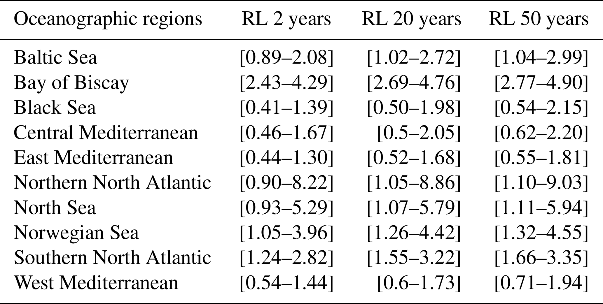
It is assumed that this collection could represent all possible short–medium return period flood scenarios affecting European coastal areas. In cases where long hindcasts or observed forcings are available, real events can be used to cover the scenarios. However, in most of the cases the real events are not sufficient, and therefore synthetic scenarios that can be defined by nearshore forcing conditions are used to cover all possible occurrences (e.g., Sanuy et al., 2018). The synthetic scenarios of the ECFAS catalogue were based on the combination of representative TWLs and storm durations derived from the ECFAS hindcast (Melet et al., 2021; Montes Pérez et al., 2022). Five reference values of the forcing TWL scenarios, indexed from one to five (named L1, L2, … L5), were defined based on the extreme values corresponding to the 2-, 20- and 50-year return levels following the scheme in Table 2. This choice was determined by the need to increase the representativeness of low–medium-intensity events and to limit the uncertainty of the higher return period values estimated by the extreme value analysis (EVA) performed on the ECFAS hindcast, which only covers 10 years (see Sect. 2.3). The EVA was performed using the methodology proposed by Mentaschi et al. (2016), employing the 97th percentile as the TWL threshold of the dataset and a declustering criteria of 72 h for the peak-over-threshold analysis (Montes Pérez et al., 2022) (see Table 3 for the ranges of values obtained in each oceanographic regions).

Table 2 Correspondence between TWL peak and reference level (L) results from the EVA. Δ is defined as a third of the range RL2–RL20: $\mathrm{\Delta }=\frac{\mathrm{RL}\mathrm{20}\text{–}\mathrm{RL}\mathrm{2}}{\mathrm{3}}$.

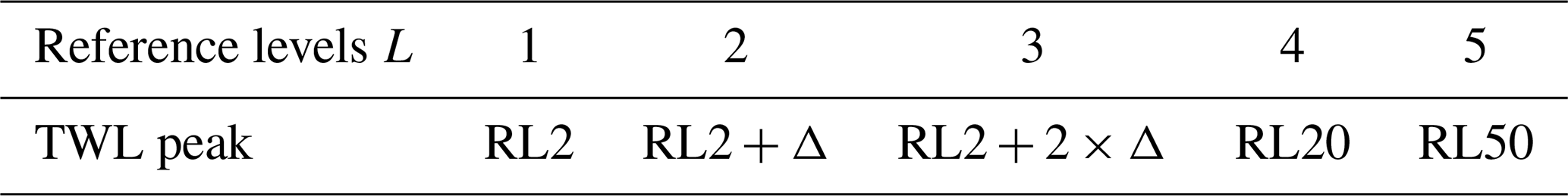
Table 3 Ranges of return levels (RLs) in meters obtained from the EVA in each oceanographic regions (Montes Pérez et al., 2022).

Three storm durations (D) – 12, 24 and 36 h – were used. These values were chosen based on an analysis of storm durations for all European coasts (Montes Pérez et al., 2022). The analysis was implemented by identifying coastal storms' start and end times following the definitions by Harley (2017), using different sets of thresholds and independent meteorological criteria. Thus, 15 scenarios were designed, representing the permutation of the five TWL peaks and three durations. Hereafter, each scenario will be referred to following the TWL reference index L and the storm duration D, such as L1D12 corresponds to the synthetic scenario with the first TWL reference level (2-year return period) and a 12 h storm duration.

From the synthetic scenarios, synthetic storms and associated TWL time series were defined. The use of synthetic storms is common practice for storm impact assessment and counterbalances a lack of observed time series (McCall et al., 2010; Santos et al., 2019; Athanasiou et al., 2021). This type of surrogate has already been suggested for coastal hazard and risk assessment (Poelhekke et al., 2016; Plomaritis et al., 2018; Sanuy et al., 2018). For this study and as illustrated in Fig. 2, the shape of the temporal evolution of the storm was assumed to follow a symmetric triangle above a level identified as the “duration threshold”, defined following the duration analysis mentioned above. The 6 h spin-up and spin-down times were added at the beginning and the end of the simulation to reach the duration threshold from 0 m to return. A more elaborate shape to represent the temporal approximation of the TWL has been suggested, such as by MacPherson et al. (2019). They used a stochastic approach to define synthetic events for 45 locations in the German Baltic Sea based on data varying between 14 and 66 years. For the present study, the application of such a sophisticated method at European scale was not possible, and it is for the sake of simplicity at European scale that the symmetrical triangle shape was chosen. The parameters, TWL peak and storm duration, were defined at each coastal point of the ECFAS combined hindcast grid with a 2.5 km resolution. As the boundary conditions of the flood model were applied at the mesh coastline at a 100 m resolution, the parameters were interpolated using the nearest-neighbor method. For each coastal sector, flood models were developed for each of the 15 defined scenarios, leading to 15 flood maps per coastal sector.

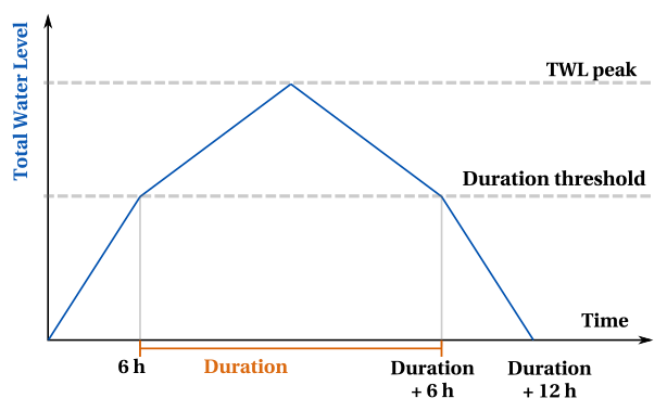
Figure 2 Definition of the synthetic storm used for forcing the flood model. TWL peaks and durations were derived from the extreme value analysis results and duration analysis.

3.4 Evaluation of the ECFAS catalogue representativeness

To assess the capacity of the catalogue to represent real events, and thus to validate the approximation of the total water level by the defined synthetic storms, the M.F.A. simulated by models forced by real and synthetic storm time series were compared. Five events were considered: Xynthia at La Faute-sur-Mer (FR, 2010), Xaver at Norfolk (UK, 2013), Saint-Agatha and Vaia at Lido Delle Nazioni (IT, 2014 and 2018), and Emma at Cadiz (ES, 2018). To generate the synthetic maps, the closest synthetic storms (as defined in Sect. 3.3) to the real time series were selected to force the model. The same skill scores (C, H and F described in Sect. 3.2) estimated for the validation against satellite-derived flood maps were used by taking as reference the flood model from the real time-series forcing.

3.5 Assessment of flood patterns across Europe and connections to LU/LC environments

For each scenario and coastal sector, the surface of the M.F.A. was estimated from the ECFAS catalogue. Their differences between the scenarios show the sensitivity of the concerned coastal sector to the TWL peak or duration changes and therefore allow the identification of patterns along the European coasts. Considering the relative change in the M.F.A. between peak levels one and five for a 24 h storm duration, normalized by the relative increase between the average peak of the TWL, the ratio α was defined as

$$\begin{array}{}\text{(5)}& \mathit{\alpha }={\displaystyle \frac{{\mathrm{MFA}}_{\mathrm{L}\mathrm{5}\mathrm{D}\mathrm{24}}-{\mathrm{MFA}}_{\mathrm{L}\mathrm{1}\mathrm{D}\mathrm{24}}}{{\mathrm{MFA}}_{\mathrm{L}\mathrm{1}\mathrm{D}\mathrm{24}}}}\times \stackrel{\mathrm{‾}}{{\displaystyle \frac{\mathrm{TWL}{\mathrm{peak}}_{\mathrm{L}\mathrm{1}}}{\mathrm{TWL}{\mathrm{peak}}_{\mathrm{L}\mathrm{5}}-\mathrm{TWL}{\mathrm{peak}}_{\mathrm{L}\mathrm{1}}}}}.\end{array}$$

A α higher than 100 % means that the maximum flooded area increased more than the water level, while for values smaller than 100 %, the flood extent did not increase as much as the water level peak.

In order to connect the flood pattern and sensitivity with LU/LC environments, the flood maps were overlaid on the LU/LC Coastal Zone 2018 data, and a relative distribution of the LU/LC first-level class environments inside the flooded area was estimated for each coastal sector.

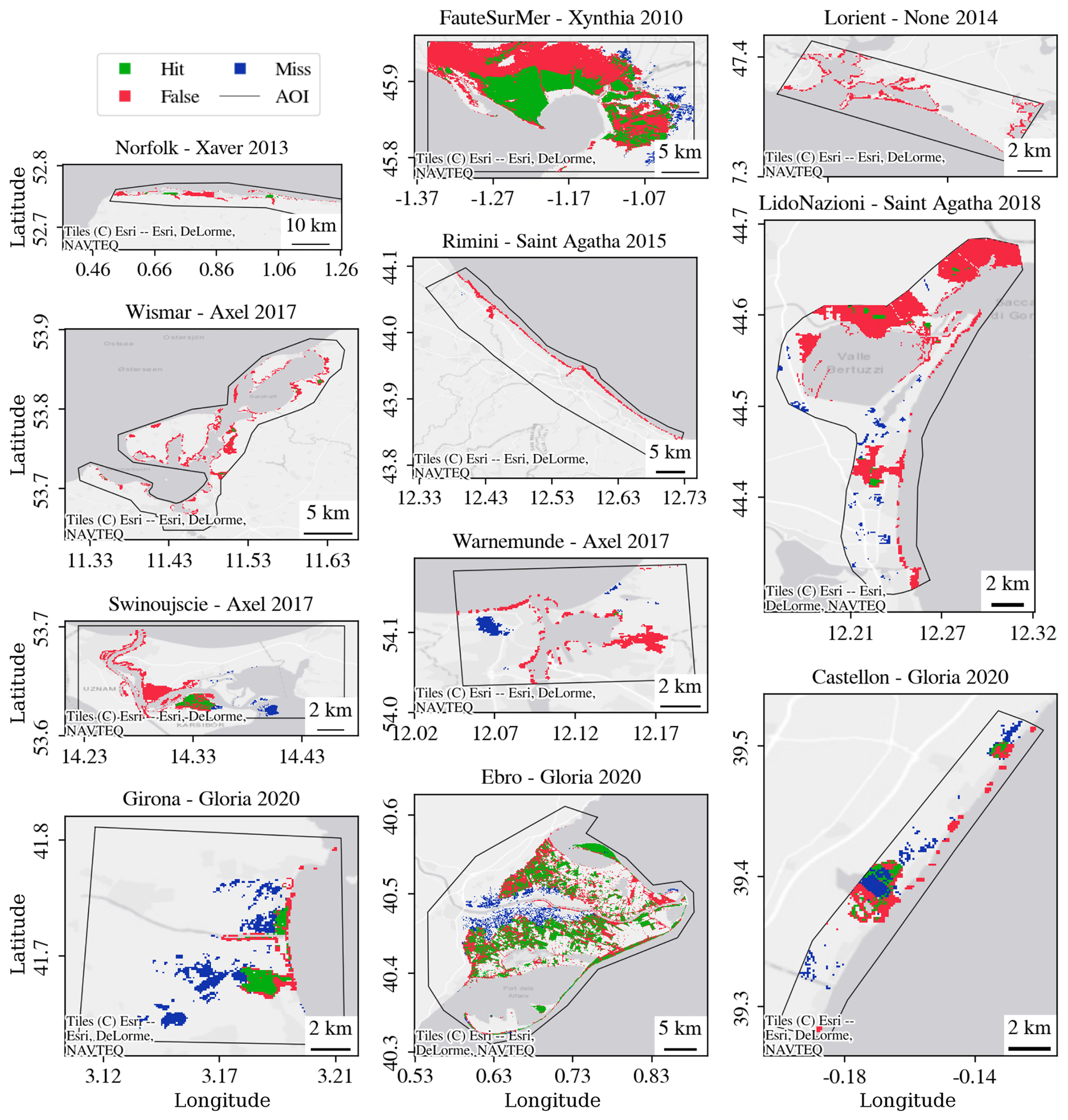
Figure 3 Performance of the model for each test case. The green areas match the intersection of the satellite-based and modeled flood (H), the blue represents the missed flood of the modeled flood, and the red areas are the flooded areas predicted by the model but not in the satellite-based flood (F). The black polygons correspond to the area of interest (AoI) that was defined to extract the satellite-based data. The background maps were generated using the ESRI database available through Python (Open Database License).

4 Results

4.1 Validation against observed data

By direct comparison between the modeled and satellite-based maps (Fig. 3 and Table 4), the flood model overpredicted the flooded area, as eight test cases have a F>100 % and four above 1000 %. The global scores C are low, from 0 to 47 %, but H scores are high: half of the test cases have H>80 % (see Fig. 3 and Table 4). The best score C is reached for the test case at the Ebro Delta during the storm Gloria (2020), C=47.67 %, while a null C is estimated for the model at Rimini during Saint-Agatha (2015). The best hit score is obtained for the test case at Norfolk during Xaver (2013), H=99.75 %, and the worst again is at Rimini during Saint-Agatha (2015), H=0 %. The overestimation witnessed in the results should be considered in the context of the available observed data. A close examination of the observed maps revealed some gaps in the observations: while observable flooded areas are identifiable away from the coastline, they are not identifiable in between, suggesting the presence of missing areas. This is particularly true for the test cases concerning Vaia 2018 at Lido Nazioni, Xaver 2013 at Norfolk and Gloria 2020 at Castellon (Fig. 3). As a result, the present satellite-based maps indicate the presence of flooded waters more than precise flood extents. Acknowledging this limitation leads to the validation of accurately represented observed flooded areas rather than focusing solely on global flood model accuracy, which could favor overpredicting models. This aspect is further discussed in Sect. 5.1. Concerning the comparison with the flood markers (Table 4), 5 test cases out of 10 have a marker hit score H_m of 100 % and one at 94.11 %. Only three test cases flooded less than half of the markers, and only the test case at Castellon during Gloria (2020) hit none of them.

Table 4 Flood model skill scores (C, H, F, H_m) for each test case in comparison to observed data. The x means that there is no reference data to estimate the score.

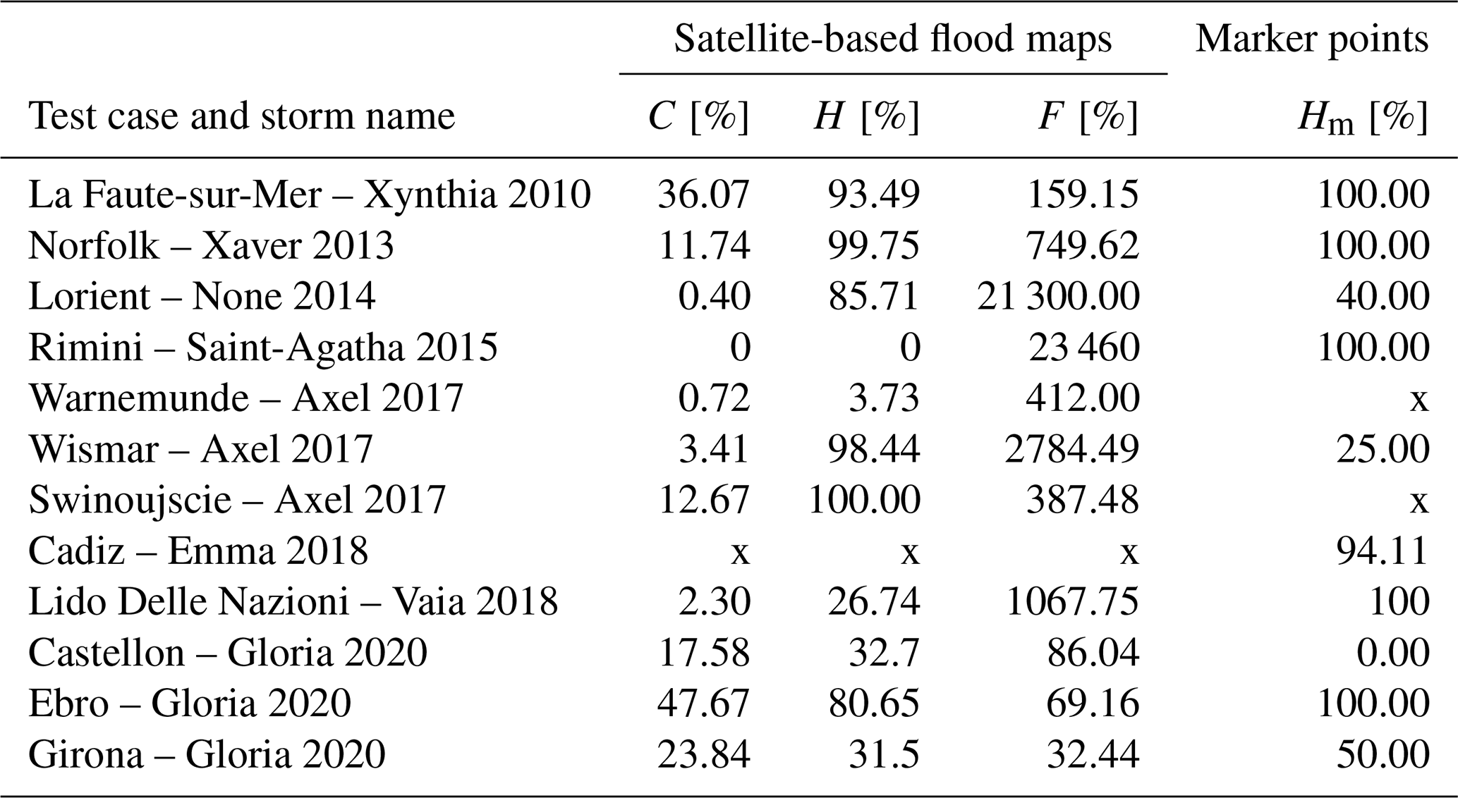
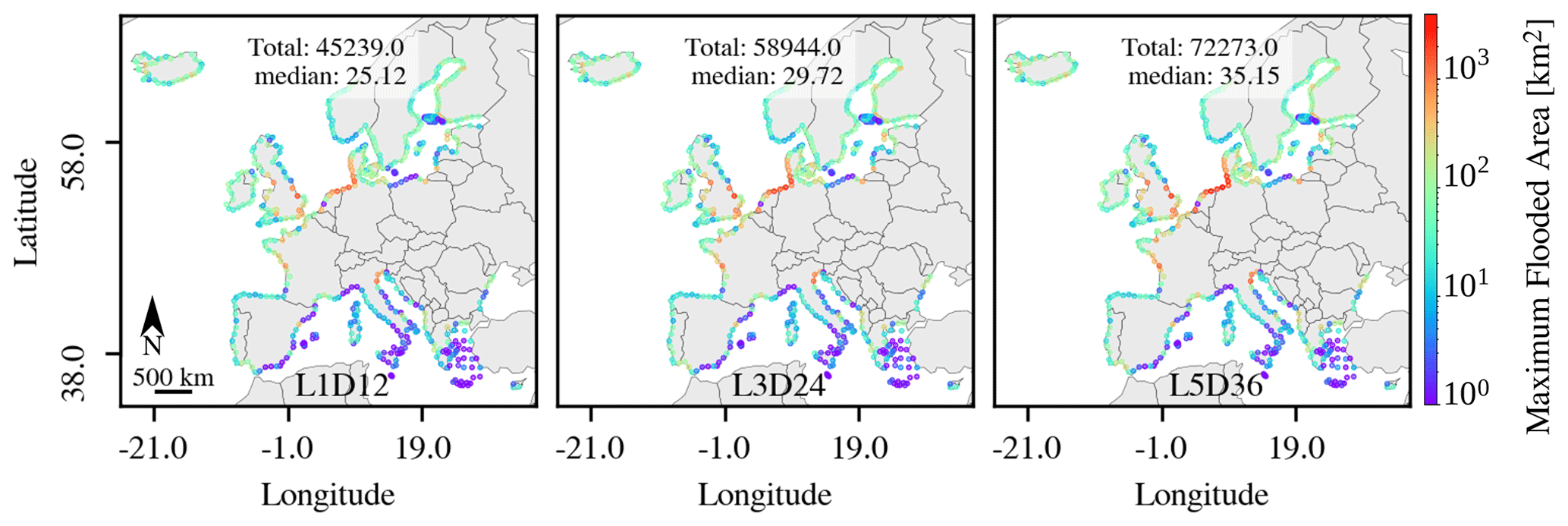
Figure 4 Catalogue maximum flooded areas for L1D12, L3D24 and L5D36 scenarios and for each coastal sector (in km²).

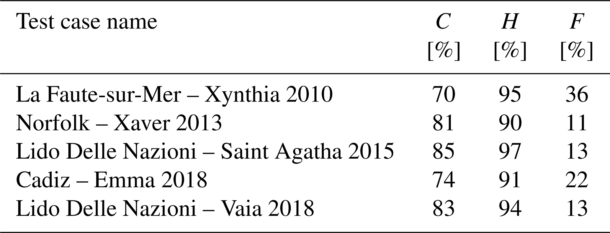
4.2 Assessment of the catalogue representativeness

As mentioned in Sect. 3.4, the value of the flood catalogue relies on the definition of the synthetic extreme events and TWL time series, as well as their capacity to represent real events. To assess the reliability of the catalogue, the flood maps of the closest TWL synthetic scenario from the catalogue were compared to those generated by flood models forced by realistic water level time series extracted from the ECFAS hindcast (Sect. 2.3), and the C, H and F indicators were evaluated (see Table 5). The global scores C are above 70 %, with a hit score H larger than 90 % and a false score between 10 % and 40 %. Even if the maps derived from the synthetic storms seem to miss some relatively small areas, particularly at Lido Delle Nazioni (not shown), they tend to slightly overpredict the flood extent, especially at La Faute-sur-Mer and Cadiz, for which the F ratios are 36 % and 22 %, respectively.

Table 5 Catalogue skill scores (C, H, F) for the closest scenario in comparison to real time-series models.

4.3 Flood spatial variability from the ECFAS catalogue

Through the different scenarios, the most affected areas are on the continental North Sea coast (from the Netherlands to Denmark), which is exposed to the highest water level peaks and where there is a high density of flood-prone areas (Fig. 4). In addition, other smaller areas are highlighted, especially around estuaries such as the German Bight, the northern part of the Adriatic Sea (Po river), the Gironde estuary (FR), the Bristol Channel, the Solway Firth and the Thames Estuary (UK).

For all coastal sectors, the maximum flood extent increases along with the reference level and duration. The accumulated total flood extent for the whole zone varied between 45 239 and 72 239 km² for the weakest (L1D12) and strongest (L5D36) scenarios, respectively.

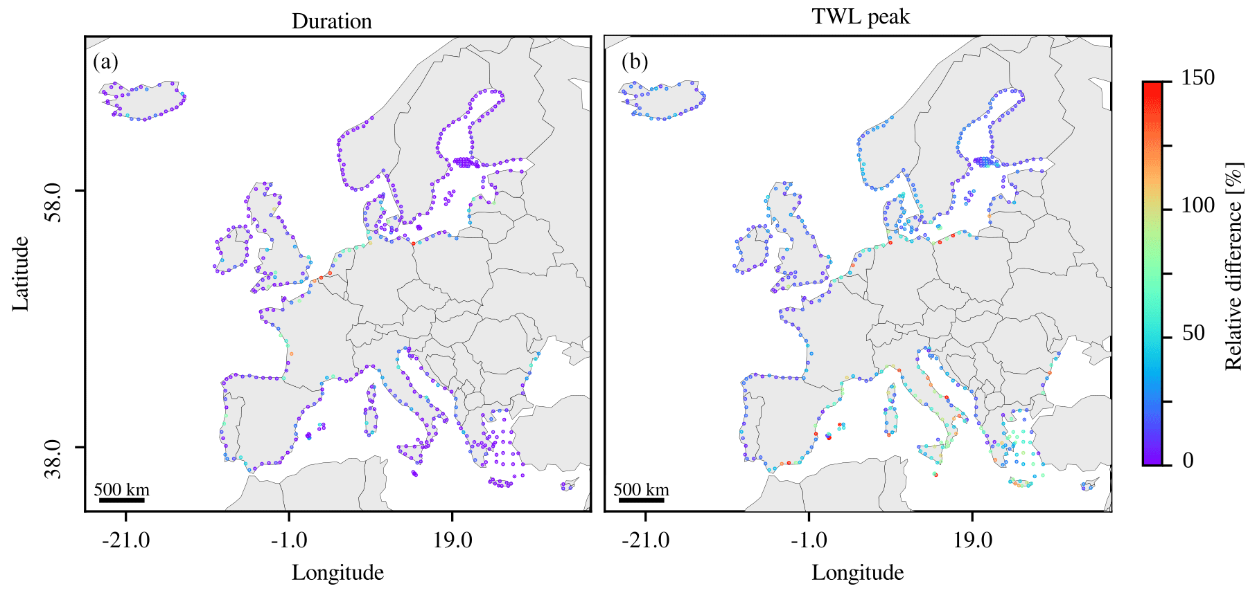
Figure 5 Maps of relative M.F.A. differences between the synthetic storm L4D36 and L4D12 scenarios (a) and between L1D24 and L5D24 scenarios (b).

It is also interesting to note that the different coastal sectors do not evolve similarly with the change in the water level and storm duration (Fig. 5). Indeed, the increase in the duration from 12 to 36 h especially impacts the Dutch coast, the Elbe and Gironde estuaries, and the Swinoujscie area (Poland), with flood extent increasing more than 100 %. In addition, a few coastal sectors encapsulating estuaries – the Po, Rhone and the central coast of Portugal (encompassing the Mondego estuary and Aveiro Lagoon) – are also sensitive to the storm duration, with an increase of ∼50 % of the maximum flooded areas. The relative influence of the TWL peak is more general, especially with a relative increase of more than 50 % along the Mediterranean coasts and more than 100 % in some coastal sectors such as along the Malaga coast (south of Spain).

Concerning the relative increase in M.F.A. in comparison to that of the TWL peaks, α mainly varies between 50 % and 150 %, with a median at ∼102 %, meaning that half of the coastal sectors, especially along the Mediterranean shore, witness a larger relative increase in the flood extent in comparison to the water level (Fig. 6).

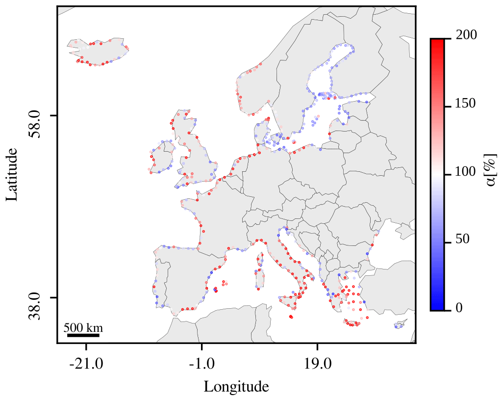
Figure 6 Maps representing the relative M.F.A. increase compared to that of TWL peaks (α) between the L1D24 and L5D24 scenarios.

5 Discussions and limitations

5.1 Validation of the flood modeling method and evaluation of the synthetic storm approximation

The assessment of the flood method accuracy was strongly constrained by the quality of the available data. The very low performance of most of the test cases could be due to partial observation of the flood event from the satellite images acquired afterwards (Tarpanelli et al., 2022). Most of the satellite images were acquired a few days after the event (from 0 to 5 d; see Table 1), by which time most of the coastal water could have already withdrawn. In addition, there are observed flooded areas that seem not related to the coastal event, especially at Girona and Wismar, for which water surfaces were extracted far from the coasts. Kiesel et al. (2023) discussed the limitations of the satellite-derived flood maps for validating purposes. In addition to the issue of the time acquisition, they highlighted the uncertainties of the method used to generate the observed maps and the possible existence of inland flood defense not integrated in the hydrodynamic models. They concluded that the metrics used to evaluate the models can leave a misleading impression on its performance. Similarly, the estimation of the present global score C was strongly biased by the misrepresentation of coastal flooding by the satellite-based data. Instead, if the hit score H is considered to evaluate the model skills, the models overall performed satisfactorily with five test cases with H>80 %. With the flood markers, the test cases gave, in the majority, satisfactory results considering that the in situ flood markers are very local data, while the methodology used for the test cases was configured for large scale. While using the hit scores to evaluate the performance of the flood model tended to favor overprediction, it was assumed that the selected flood method correctly represented the flood process.

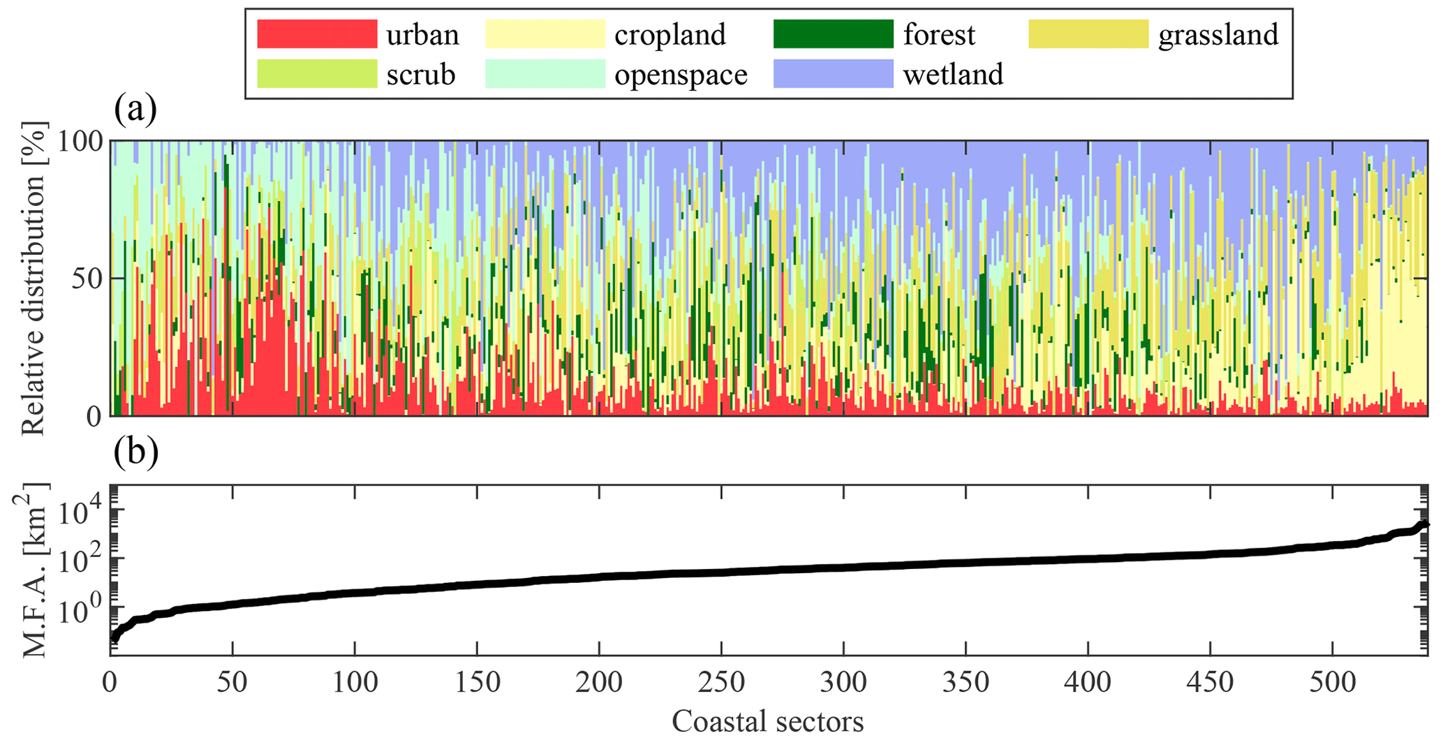
Figure 7 Relative distribution of the first-level land use and land cover classes as defined by the LU/LC Coastal Zone 2018 database (Innerbichler et al., 2021) in the flooded area for each coastal sector (a). The coastal sectors are sorted by ascending maximum flooded area for synthetic scenario L4D24 (b).

Concerning the comparison between real and synthetic storm time series, the synthetic storm maps accurately approximated the flood maps derived from real time series. This confirms the robustness of synthetic storm approximation for the selected events and supports the choice of a simple symmetrical triangle approximation of the extreme events instead of a more elaborate shape. However, this accuracy is bound to the events that were simulated, as the triangular symmetrical shape used for the synthetic storm may not be a good representation of real storms in other locations (Duo et al., 2020). Nonetheless, the list of test cases gathered various morphologies and oceanographic conditions (on the Atlantic coast, in the North and Adriatic seas), and it was then accepted that this result can be extrapolated at European scale and that the synthetic storms defined to generate the ECFAS flood catalogue were suitable approximations.

5.2 Flood spatial variability from the ECFAS catalogue and connection to LU/LC data

The highlighted areas exposed to the larger flood extents (Fig. 4) are similar to those identified by Vousdoukas et al. (2016) and Paprotny et al. (2019). The largest floods are correlated with flood-prone areas such as well-known low-lying areas (Dutch coast) and wetlands. Considering the relative distribution per coastal sector of the LU/LC data, as defined by the first-level class of Coastal Zone 2018 (see nomenclature in Innerbichler et al., 2021), the maximum flooded area increases with wetland and cropland areas (Fig. 7). At the same time, coastal areas with important urban areas and open space with little vegetation, among beaches and dunes, are those that witness the smallest floods.

The models of Vousdoukas et al. (2016) and Paprotny et al. (2019) were forced by synthetic storms corresponding to a return level of 100 years with durations varying with the coastal sector. Also using a 100 m flood model, Vousdoukas et al. (2016) obtained a total flood extent of ∼30 696 km², significantly smaller than any of the present total estimations for the largest peak scenario (i.e., matching the 50-year return level). This important discrepancy can be explained, in addition to the model configuration differences (synthetic storm shape, DEM, etc.), by the fact that the coastal defenses were not included in the present work, and the most exposed areas (from Netherland to Denmark) have the highest protection in Europe (∼15 m as design total water levels; see Vousdoukas et al., 2016). This represents a limitation of the current estimation of flooded areas since only features appearing in the 10 m DEM, downscaled at 100 m, are represented in the model grids.

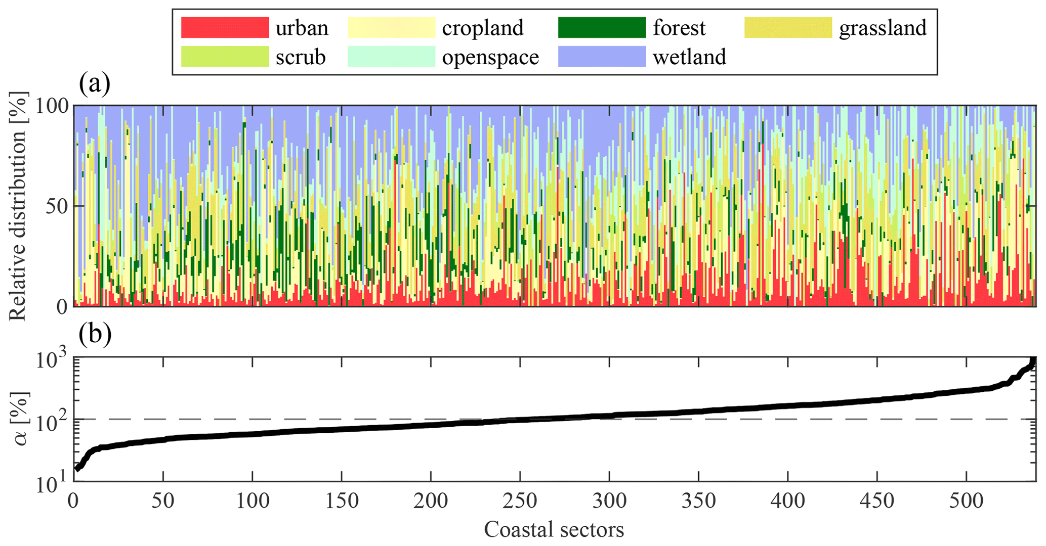
Figure 8 Relative distribution of the first-level land use and land cover classes as defined by the LU/LC Coastal Zone 2018 database (Innerbichler et al., 2021) in the flooded area for each coastal sector (a). The coastal sectors were sorted by ascending α, being the relative difference in the maximum flooded areas compared to the relative TWL peak increase between scenarios L5 and L1 for the 24 h storm duration (b).

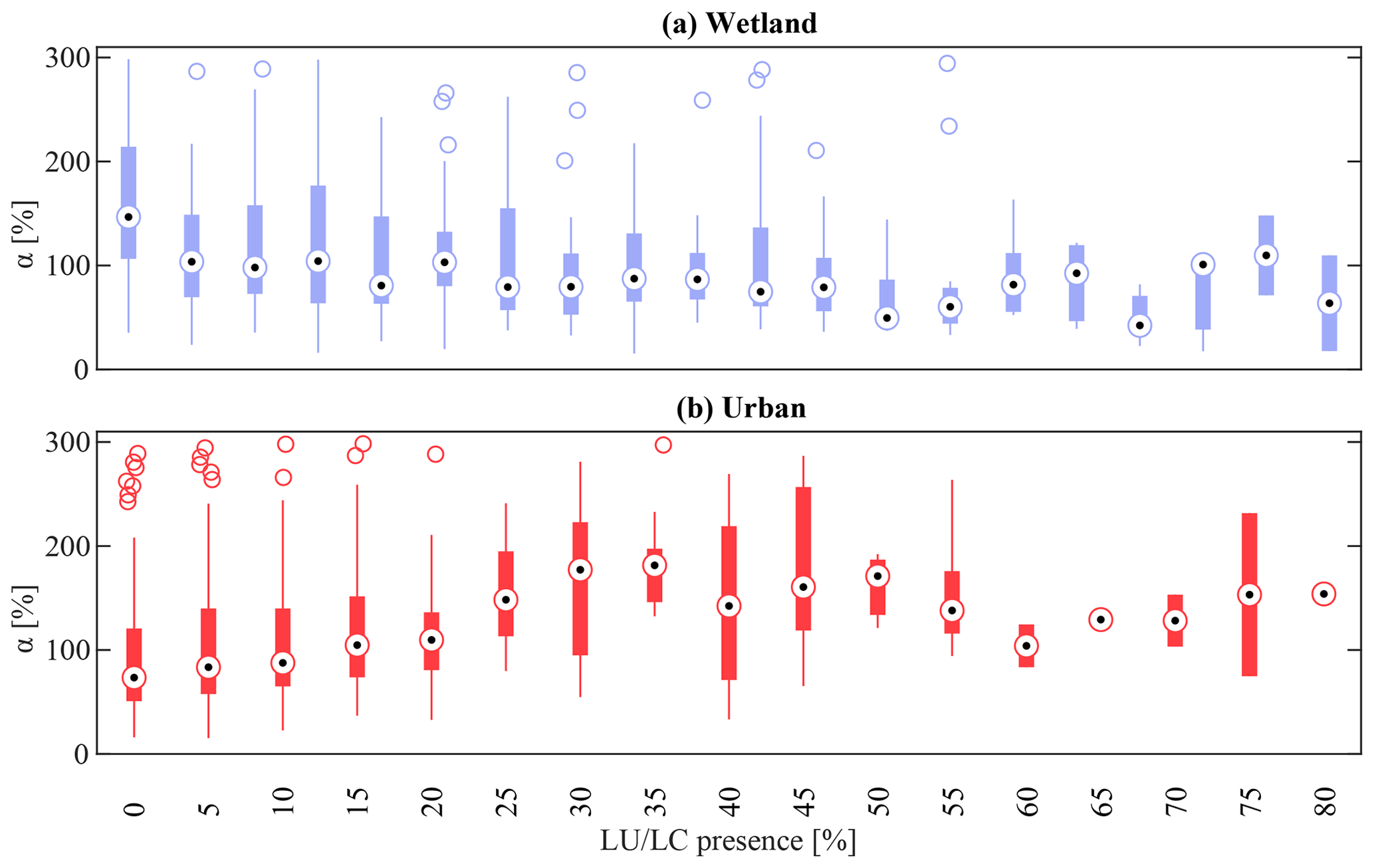
Figure 9 Evolution of α depending on the relative presence of wetland (a) and urban (b) environment in the maximum flooded areas of the scenario L5D24 for each coastal sector. The black dot, thick line, thin line and single circles represent the median, the 25th and 75th percentiles, the minimum and maximum, and outliers for every 5 % bin, respectively.

Concerning the relative increase in M.F.A. compared to that of TWL peaks, α, globally, no regional trend can be identified (Fig. 6). However, the flooding of the coastal sectors in the Baltic Sea seems less sensitive to the increase in the water level peak than the Mediterranean predictions are. The coastal sectors with high α are similar to those sensitive to the increase in the water level in Fig. 5b. Similarly to the M.F.A., the distribution of the LU/LC in the flooded area depending on α could indicate environments that mitigate flood spread and act as buffer zones for coastal flooding (see Fig. 8). Qualitatively, urban areas are more sensitive than coastal sectors with large flooded wetland surfaces. A few coastal sectors present very high α due to very small or null flooded areas for the reference scenario. These outliers were identified through the median absolute deviation method and excluded for the following analysis. The evolution of the median of α, every 5 %, depending on the wetland and urban relative presence in the M.F.A., shows negative and positive trends (see Fig. 9). This is confirmed by a significant correlation of $\sim -\mathrm{0.29}$ ($p\sim {\mathrm{10}}^{-\mathrm{11}}$) and of $\sim +\mathrm{0.27}$ ($p\sim {\mathrm{10}}^{-\mathrm{10}}$) between α and the wetland and urban distributions, respectively. The wetland and urban areas differ in the model by the local topography and slope and also by Manning's friction coefficient that is imposed, as stated in Sect. 2.2. The identified urban areas have a Manning coefficient of 0.013 s m${}^{-\mathrm{1}/\mathrm{3}}$ and those of wetlands of 0.04 s m${}^{-\mathrm{1}/\mathrm{3}}$. Thus, the friction is stronger in wetlands than in urban areas. Hence, considering friction alone, water propagation will spread more easily in urban areas once reached. Coastal flood mitigation by wetlands has already been highlighted numerous times and reviewed by Leonardi et al. (2018). Thus, the present catalogue brings a global European perspective to this matter that was usually studied at local or regional scale (Smolders et al., 2015; Stark et al., 2015, 2016). From a global perspective, Van Coppenolle and Temmerman (2020) identified the Wash Bay (UK) and the Elbe Estuary as two major hot spots in Europe where the coastlines benefit from wetland mitigation. In the present study, α was estimated to be ∼40 % at the Wash Bay, also showing a low sensitivity to the water level increase. However, α was estimated to be higher than 300 % for the coastal sector with the Elbe Estuary. This could be due to the dynamic of the river (Winterwerp et al., 2013) channeling the flood propagation that is not considered by Van Coppenolle and Temmerman (2020), as well as the partial representation of the wetland due to the coastline approximation in the present model. Indeed, with the current setup and the approximation of the boundary position, tidal flats are modeled by the combined hindcast with a 2.5 km resolution, which is not sufficient to fully represent this local complex dynamic (see Sect. 5.3 for the limitations of the ECFAS catalogue).

5.3 Limitations of the ECFAS catalogue

The development of the ECFAS flood map catalogue resulted from a balance between accuracy and computational feasibility (Paprotny et al., 2019) to provide large-scale coastal flood assessment for European coasts. While the general method was supported by validations, some approximations could limit the correctness of the present study. First, the flood extent estimation is limited by the quality of the input data, such as the DEM, with a resolution of 10 m that was coarsened to 100 m in the modeling setup. This leads to a loss of local topography representation and may flatten out local higher ground or coastal defenses. Therefore, the flood in some areas, such as along the Dutch coast, could be overpredicted. In addition, no human-made flood protection structures were integrated from specific databases (Vousdoukas et al., 2016), meaning that only those detected from the satellite images and, therefore, included in the DEM were considered.

Another major limitation is in the approximation of the boundary position, which is directly derived from the numerical grid and, therefore, the DEM and waterbody mask files. This led to two identified issues. Firstly, the boundary position is static, not considering morphodynamic processes such as erosion that could affect the entity of the forcing. The erosion of the beach profile has a positive feedback on the water volume entering the hinterland and should be taken into account for coastal flood modeling even for regional-scale studies (Viavattene et al., 2018). Secondly, the forcing is applied at the mouth of estuaries, where the interaction between estuarine circulation and incoming waves is not accounted for. Indeed, in the present configuration, the flood model does not integrate the river dynamics and even the tides are schematized in a rough way, given the resolution of the global bathymetry. The model uses the acceleration flood-plain solver, only partially solving the shallow-water equations, to propagate the surge inside the river mouth. It is then expected that the inundation propagation is not well represented in such areas. However, to take these aspects into account, more detailed datasets and local approaches, such as surge coastal propagation, are needed.

Concerning the catalogue scenarios, they are based on return water levels and storm durations derived from extreme value and duration analyses applied on the ECFAS combined hindcast. However, this hindcast considered only a decade of data reconstructing the TWL by linear addition of its components, excluding the run-up component and discarding nonlinear interactions with a model resolution of 2.5 km at the coast. These accumulated approximations could decrease the robustness of the identified return levels. The use of the synthetic storms also contributes to the limitations of the current model. Although it represents a common practice, as pointed out in Sect. 3.3, the use of triangular-shaped storm time series can lead to non-reliable results such as for wave-driven coastal storms in the Mediterranean, as demonstrated specifically for symmetric triangular synthetic storms by Duo et al. (2020).

6 Conclusions

A pan-European flood catalogue collecting flood maps was produced for 15 medium–high-frequency synthetic scenarios with representative forcing parameters for each coastal sector. The scenarios combined storm surge, wave setup and storm duration data, adding a new dimension to the existing databases in the literature. A dynamic method was applied to model the surge propagation inland, and the flood modeling method was evaluated with 12 test cases spread across Europe. While this analysis was strongly restrained by the limitation of the observed satellite-based data, biasing a global estimation of the accuracy of the models, it was found that the models quite correctly represented the observed flooded areas and markers. In addition, the approximation of water level real time series using synthetic storms was proven to be satisfactory by comparing flood maps from the closest synthetic scenario with those based on real time series for five events/sites.

At European level, most of the flooded area was concentrated on the North Sea and additional singular locations that were connected to flood-prone configurations, regardless of the TWL peak and storm duration. As the present analysis does not integrate any coastal defense, with the exception of those included in the DEM, the present estimation could be overpredicted.

The results across the synthetic scenarios showed different sensitivity to the increase in the water level and the duration. While the duration mainly influences the areas identified with large flooded areas, the TWL peak is particularly impactful on the Mediterranean coasts. In addition, most of the coastal sectors, except those in the Baltic Sea, witnessed a relatively larger increase in the flooded areas than the water level, meaning that every small water level rise could lead to more dramatic flooding. In this regard, it was found that wetlands tend to reduce this sensitivity and mitigate the flood spread, while the coastal sectors with larger flooded urban areas are subjected to a higher flooding increase with the TWL peak.

The identified limitations of the ECFAS catalogue were mainly correlated to the quality of the input data and the approximations driven by the need to balance between accuracy and computational feasibility. This mainly concerned the missing coastal defenses and the approximation of the forcing conditions at the coastlines. Therefore, the ECFAS catalogue does not pretend to replace any local or national flood hazard estimation. Nonetheless, considering the lack of global flood hazard assessment targeting high-frequency (low to medium intensity) events at European scale, the present flood map catalogue fills this gap and permits an assessment of the potentially frequent coastal flood hazards along European coasts. In this way, it could be used in the prevention phase to analyze scenarios and disaster risk reduction strategies or during preparedness phases, supporting EWSs along with an operational forecasting system for nearshore forcings as proposed by the ECFAS project.

Appendix A: Manning coefficients

(Innerbichler et al., 2021)

Table A1 Manning coefficients used to generate the friction maps for the flood model. The values were directly taken from Chow (1959) and Papaioannou et al. (2018). The Coastal Zone 2018 layer is structured in up to five levels of subcategories; when sharing the same Manning coefficient and for the sake of clarity, the subcategories were aggregated into the biggest similar level annotated with ^*.