the Creative Commons Attribution 4.0 License.
the Creative Commons Attribution 4.0 License.
 | 27 Jan 2023
Evaluation of low-cost Raspberry Pi sensors for structure-from-motion reconstructions of glacier calving fronts
Duncan J. Quincey
Mark W. Smith
Glacier calving fronts are highly dynamic environments that are becoming ubiquitous as glaciers recede and, in many cases, develop proglacial lakes. Monitoring of calving fronts is necessary to fully quantify the glacier ablation budget and to warn nearby communities of the threat of hazards, such as glacial lake outburst floods (GLOFs), tsunami waves, and iceberg collapses. Time-lapse camera arrays, with structure-from-motion photogrammetry, can produce regular 3D models of glaciers to monitor changes in the ice but are seldom incorporated into monitoring systems owing to the high cost of equipment. In this proof-of-concept study at Fjallsjökull, Iceland, we present and test a low-cost, highly adaptable camera system based on Raspberry Pi computers and compare the resulting point cloud data to a reference cloud generated using an unoccupied aerial vehicle (UAV). The mean absolute difference between the Raspberry Pi and UAV point clouds is found to be 0.301 m with a standard deviation of 0.738 m. We find that high-resolution point clouds can be robustly generated from cameras positioned up to 1.5 km from the glacier (mean absolute difference 0.341 m, standard deviation 0.742 m). Combined, these experiments suggest that for monitoring calving events in glaciers, Raspberry Pi cameras are an affordable, flexible, and practical option for future scientific research. Owing to the connectivity capabilities of Raspberry Pi computers, this opens the possibility for real-time structure-from-motion reconstructions of glacier calving fronts for deployment as an early warning system to calving-triggered GLOFs.
- Article
(7484 KB) - Full-text XML
-
Supplement
(404 KB) - BibTeX
- EndNote


Monitoring glacier calving fronts is becoming increasingly important as climate warming changes the stability of the cryosphere. Globally, glacier frontal positions have receded rapidly in recent decades (Marzeion et al., 2014; Zemp et al., 2015), leading to an increased threat of glacial lake outburst floods (GLOFs) from newly formed proglacial lakes at the glacier terminus (Tweed and Carrivick, 2015), or tsunami waves and iceberg collapse at marine-terminating glaciers (Minowa et al., 2018). Large ice calving events and their impact into glacial lakes can trigger violent waves (Lüthi and Vieli, 2016) and ultimately GLOF events if the wave goes on to overtop the impounding dam, though both the magnitude and frequency of this phenomenon are poorly quantified owing to a lack of appropriate monitoring (Emmer et al., 2015; Veh et al., 2019). Satellites are able to provide near-continuous observations of lake growth (Jawak et al., 2015), hazard development (Quincey et al., 2005; Rounce et al., 2017), and, over large glaciers, calving rate (Luckman et al., 2015; Sulak et al., 2017; Shiggins et al., 2023). However, to measure frontal dynamics at a high spatial and temporal resolution, which is particularly necessary over calving glaciers, monitoring requirements can only be met by in situ sensors.
Accurate 3D models of glaciers and their calving fronts are necessary to fully evaluate the hazards they pose (Kääb, 2000; Fugazza et al., 2018) and to better understand frontal dynamics (Ryan et al., 2015). Where in situ camera sensors have been used to monitor glacier fronts as part of an early warning system, stationary cameras have previously been used to relay regular images to be analysed externally (Fallourd et al., 2010; Rosenau et al., 2013; Giordan et al., 2016; How et al., 2020). This can be useful for monitoring glacier velocity, snowfall, and calving dynamics (Holmes et al., 2021), but remains a 2D snapshot of glacier behaviour which only allows qualitative insights into calving volume (Bunce et al., 2021). 3D models, on the other hand, permit more detailed analysis and allow calving events to be quantified in size (James et al., 2014; Mallalieu et al., 2020). Unoccupied aerial vehicles (UAVs) have been used regularly to capture high-resolution 3D models of glacier fronts (Ryan et al., 2015; Bhardwaj et al., 2016; Chudley et al., 2019), but, as yet, these systems are not autonomous and are therefore dependent on an operator being present, as well as often being highly expensive (many thousands of dollars), including the staff-based cost of revisiting these sites.
Arrays of fixed cameras can be positioned around a glacier front to capture images repeatedly over long time periods. The resulting imagery can then be used to photogrammetrically generate 3D models at a high temporal resolution and analyse change over days, months, or years. Off-the-shelf time-lapse cameras provide some of the cheapest ways of reliably collecting imagery for repeat photogrammetry and have been deployed at Russell Glacier, Greenland, to monitor seasonal calving dynamics (Mallalieu et al., 2017). Elsewhere in glaciology, time-lapse arrays using more expensive DSLR-grade cameras have been used for repeat structure-from-motion (SfM) to quantify ice cliff melt on Langtang Glacier at high spatial resolution (Kneib et al., 2022). In other disciplines, time-lapse arrays for SfM have been used to monitor the soil surface during storms (Eltner et al., 2017), the stability of rock slopes (Kromer et al., 2019), and the evolution of thaw slumps (Armstrong et al., 2018), for example. The key limitation of these studies, and this setup design, is that a site revisit is necessary to collect data, and analysis is therefore far from real-time. Autonomous photogrammetry, whereby 3D models are created with no user input, is still in its infancy but shows great promise, with machine learning used to optimize camera positions (Eastwood et al., 2020), point cloud stacking to enhance time-lapse photogrammetry (Blanch et al., 2020), and user-friendly tool sets for monoscopic photogrammetry (e.g. PyTrx (How et al., 2020), ImGRAFT (Messerli and Grinsted, 2015) and EMT (Schwalbe and Maas, 2017)). Real-time data transmission is the next step in autonomous time-lapse photogrammetry, but trail cameras with cellular connectivity are many hundreds of dollars per unit, rendering this setup unaffordable for most monitoring schemes.
Raspberry Pi computers are small, are low cost, and were designed with the intention of teaching and learning programming in schools. Their ease of use and affordability means they have also been used extensively as field sensors in the geosciences (Ferdoush and Li, 2014) as the quality of their camera sensors have developed to a science-grade level (Pagnutti et al., 2017). In hazard management, Raspberry Pi cameras have been used as standalone monitoring systems to complement wider internet-of-things (IoT) networks (Aggarwal et al., 2018) and attached to UAVs to produce orthophotographs (Piras et al., 2017). In glacierized environments, the durability, low cost, and low power requirements of Raspberry Pis means they have been used to complement sensor networks, such as controlling the capture of DSLR-grade time-lapse cameras (Carvallo et al., 2017; Giordan et al., 2020) or as a ground station for UAV-based research (Chakraborty et al., 2019). However, to our knowledge, Raspberry Pis and low-cost camera modules have never been the focus of a glaciology investigation and their potential for SfM in the wider geosciences has yet to be fully realized. In addition, the flexibility provided by a fully programmable sensor could offer geoscientists the ability to tailor data acquisition and perform low-level in-field processing.
The aim of this study was, therefore, to evaluate the quality of Raspberry Pi imagery for photogrammetric processing, with a view to incorporating low-cost, high functionality sensors in glacier monitoring systems. Given that the highest accuracy glacier front 3D models gathered from photogrammetry are derived from UAV imagery (typical horizontal uncertainty of 0.12 m (0.14 m vertical) even in the absence of ground control points (Chudley et al., 2019)), we chose to use a UAV-based point cloud as our primary reference dataset. We intensively deployed both sensor systems (ground-based Pis and aerial UAV) at Fjallsjökull, Iceland, over a four-day period. As a secondary objective, we also sought to understand the limitations of Raspberry Pi by deploying Raspberry Pi sensors at a range of distances to the glacier front and removing images in the processing of point clouds to identify the fewest frames necessary for generating accurate 3D models.
2.1 Study site – Fjallsjökull, Iceland
Fjallsjökull is an outlet glacier of Öræfajökull, an ice-covered volcano to the south of the wider Vatnajökull ice cap, in south-east Iceland (Fig. 1). Recession and thinning of Fjallsjökull has been underway since the end of the Little Ice Age, but has substantially accelerated in recent decades owing to climate warming (Howarth and Price, 1969; Chandler et al., 2020). Fjallsjökull terminates in a large (∼4 km2) proglacial lake – Fjallsárlón – which is also increasing in size as Fjallsjökull recedes (Schomacker, 2010). Calving of Fjallsjökull is regular and has increased in frequency in recent decades as the glacier has accelerated, driven by the expansion of Fjallsárlón (Dell et al., 2019). As of September 2021, the calving face of Fjallsjökull was approximately 3 km wide, with ∼2.4 km of this accessible from a boat (the northernmost 600 m had large, stationary icebergs which were dangerous to navigate; see Fig. 1). We selected Fjallsjökull as a study site due to its accessibility, ability to conduct surveys from boat and shoreline, and variation in calving margin heights (ranging from ∼1 to ∼15 m) to test the performance of our camera system under a diverse range of glaciological settings.
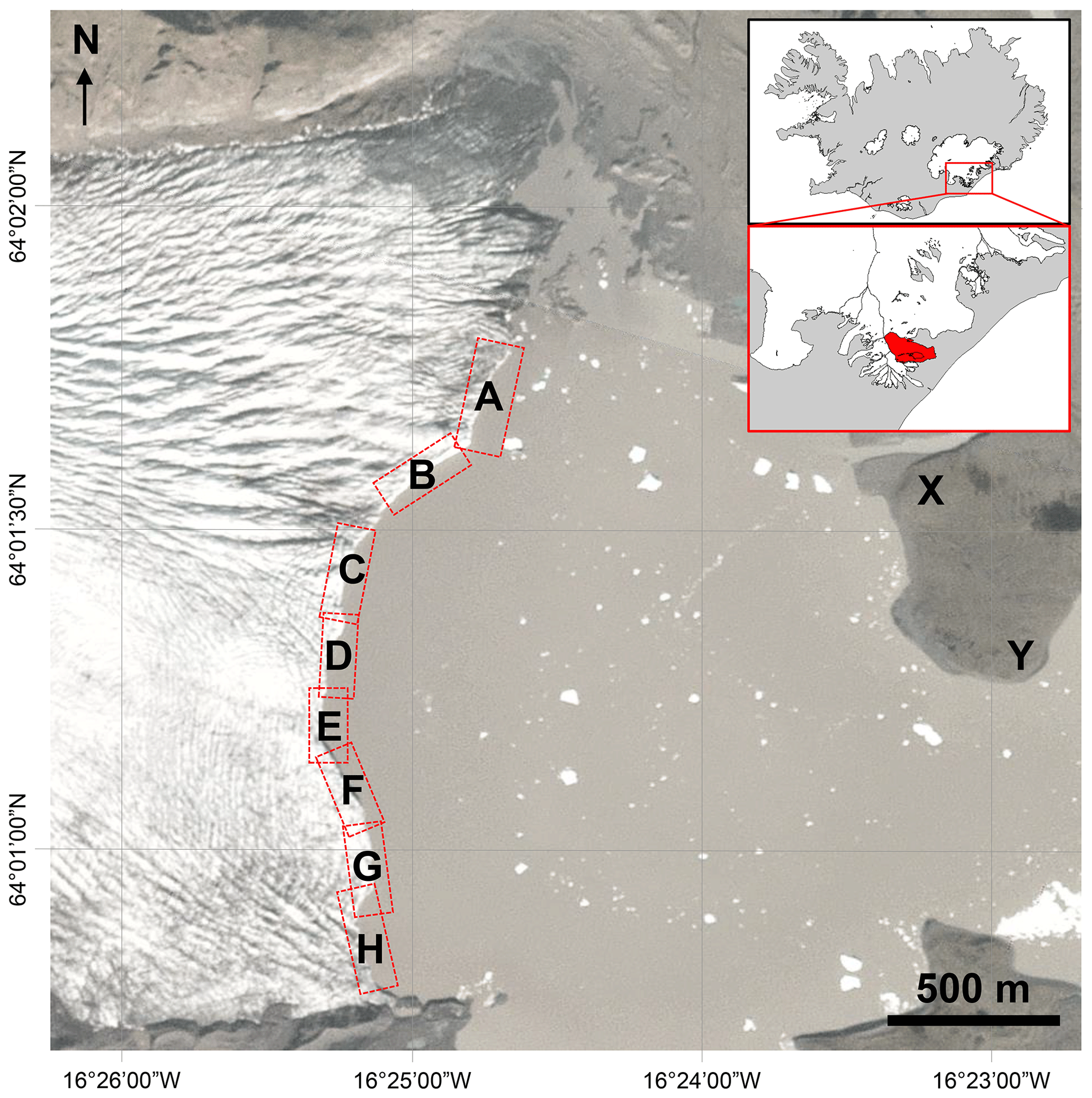
Figure 1Fjallsjökull (flowing left-to-right), terminating in Fjallsárlón, captured by Planet Imagery on 10 September 2021. A–H denote the eight point cloud sub-sections generated by both the Raspberry Pi and UAV. X–Y denote the start and end of land-based data collection at approximately 25 m intervals along the shoreline, used to generate sub-section B from a distance.
2.2 Hardware and survey details
We tested the Raspberry Pi high quality camera module with a 16 mm telephoto lens in comparison to images taken from a DJI Mavic 2 Pro UAV. We also tested the Raspberry Pi camera module V2 (of lower resolution, but a cheaper option), due to its science-grade radiometric calibration (Pagnutti et al., 2017), but initial tests indicated the quality of the long-range imagery was too low to proceed with generating 3D data. The Raspberry Pi camera was attached to a Raspberry Pi 4B computer with an LCD display to visualize images, and adjust focus, as they were captured. Technical comparisons of the setups are given in Table 1, and a list of components and our code for acquisition is given as Supplementary Information.
Table 1Comparison of technical specifications between Raspberry Pi and UAV sensors. Two typical time-lapse packages are provided as a comparison, following the setup from Mallalieu et al. (2017), using the MMS model of their wildlife camera to compare like-for-like connectivity with the Raspberry Pi, and Kienholz et al. (2019). The Raspberry Pi high quality camera module is fitted with a 16 mm telephoto lens. N/A stands for not applicable.
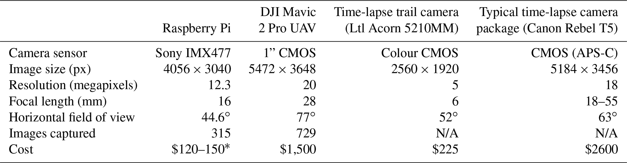
∗ In this study, we used a more expensive Raspberry Pi computer (4B) in order to fit a screen for in-field monitoring of images at a cost of USD 150, however the USD 120 cost applies to a cheaper model (Zero W).
The Raspberry Pi was mounted in a fixed position on a boat which traversed the southernmost ∼2.4 of the ∼3 km Fjallsjökull calving face, around 500 m from the glacier, while the UAV flew above this boat (Fig. 2). The Raspberry Pi was triggered manually approximately once every 10 seconds throughout the transect, capturing 315 images in total. While we operated the system manually herein, it is important to note, however, that the system is also designed to trigger autonomously at any frequency desired by the user. At the same time, the UAV conducted two flights, capturing 729 images, ensuring no calving occurred between collecting data from the two sensors. The UAV flew closer (∼250 m) to the glacier terminus than the boat transect to ensure the highest possible accuracy in data collection and to keep researchers at a safe distance to an active calving margin. This echoes similar approaches in studies of coastal landslides (Esposito et al., 2017) where a UAV flew closer than a boat survey to obtain the best possible quality 3D models for sensor comparison. In the majority of images, the UAV camera was facing the flat calving face of the glacier. While the UAV has onboard software to autofocus images, we manually checked and altered the focus of the Raspberry Pi camera between images during the boat transect to ensure pictures were not blurry as the boat varied in distance from the glacier.
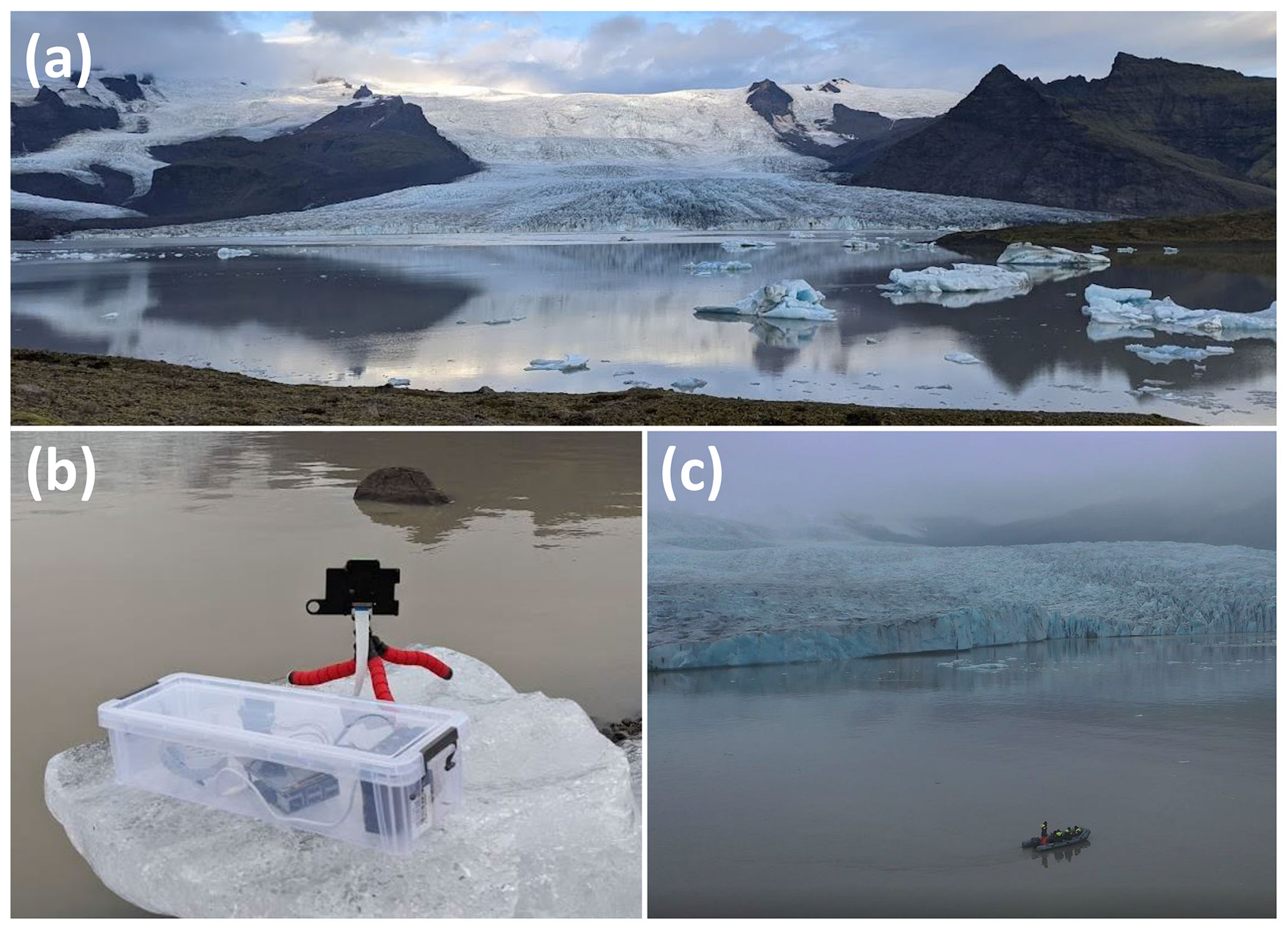
Figure 2An overview of our data acquisition. (a) Fjallsjökull, leading into Fjallsárlón, as of 17 September 2021. (b) Raspberry Pi on the shoreline survey. The camera was stabilized with a small tripod, with hardware and batteries connected in a weatherproofed receptacle. (c) Boat survey, approximately 500 m from the glacier front, as captured by the UAV.
In order to test the limits of the Raspberry Pi, we performed additional analysis on sub-section B (Fig. 1). We collected images of the calving face from a portion of the shoreline of Fjallsárlón, shown as X to Y in Fig. 1, which ranged from 1.2 to 1.5 km from the calving face. Owing to bad weather, we only collected shoreline data for a limited section (covering sub-section B entirely) before the glacier was obscured from view by fog. This experiment allowed us to assess how the Raspberry Pi performed at long-range.
We also conducted an additional experiment on sub-section B to determine the performance of the camera under sub-optimal conditions by removing 21 of the 31 images captured by the boat transect and deriving point clouds from the remaining 10 camera positions. This reflects the reality of the trade-off between data quality and practical considerations. In theory, fewer images should result in a lower point density (Micheletti et al., 2015), but any time-lapse camera array produced using Raspberry Pis could be cheaper with fewer cameras required.
2.3 Photogrammetry and M3C2
For images from both the Raspberry Pi and UAV, far cliffs (rock faces flanking Fjallsjökull; Fig. 2a) were masked out prior to generating tie points in Agisoft Metashape. Images from the UAV were georeferenced using its onboard GNSS real-time kinematic positioning (RTK) system, with an accuracy <2 m (Nota et al., 2022). Images from the Raspberry Pi were georeferenced by aligning them to images captured by the UAV and producing a sparse point cloud, before removing UAV images to produce the final dense point clouds. Point clouds from both sensors were therefore referenced to this RTK system only, rather than having a global reference (akin to Luetzenburg et al., 2021). While the Raspberry Pi images could be successfully aligned without UAV images, our workflow was designed to unify the coordinate systems of the point clouds and thereby avoid confounding co-registration errors in the cloud comparison. Eight high quality point clouds were produced from each of the Raspberry Pi and UAV at various stages along the calving face (locations in Fig. 1) with a mild depth filter using Agisoft Metashape. Sub-sections were computed at natural break points in the glacier front geometry, at approximately 250–350 m intervals, owing to limitations in computer processing. We then cropped point clouds to the calving face, cleaned with a noise filter, and finely aligned the Raspberry Pi clouds to the UAV clouds assuming a 95 % overlap in CloudCompare.
Differences between point clouds from the Raspberry Pi and UAV were compared using the multiscale model to model cloud comparison (M3C2) tool in CloudCompare (Lague et al., 2013). M3C2 calculates a series of core points from the Raspberry Pi cloud and quantifies the distance to the UAV cloud about those points using projection cylinders. This requires users to define key parameters, including the width of normal (D), projection radius (d), and maximum depth of the cylinder (h) (all parameters in metres). We followed approaches developed by Lague et al. (2013), and applied to glacierized environments by Westoby et al. (2016) and Watson et al. (2017), of calculating the normal width to take into consideration surface roughness and the scale of the model. We used a standardized value of 0.6 m across all models as this fell within the range of 20–25x surface roughness for the vast majority (>98 %) of points, following equations presented in Lague et al. (2013). Projection diameter was calculated as a function of point density, so to ensure each projection cylinder had a minimum of five points, we used a value of 1.1 m. Finally, we set the maximum projection depth to 10 m to exclude grossly erroneous values (<0.01 % of all values).
3.1 Use of Raspberry Pi cameras in generating point clouds
The Raspberry Pi-based camera captured high-resolution imagery across the full length of Fjallsjökull, at distances of up to 1.5 km. Glacier textures and structures, such as debris patches and cracks in the ice, were clearly visible within the photos captured by the Raspberry Pi (see example imagery in Fig. 3) to aid 3D reconstruction. The ground sampling distance (GSD) (the on-ground distance represented by one pixel) of the Raspberry Pi at 500 m range was 3.80 cm and at 1.5 km was 11.41 cm (following calculations by O'Connor et al., 2017). By comparison, trail cameras used by Mallalieu et al. (2017), at a mean distance of 785 m to Russell Glacier, achieved GSD of 28.05 cm. We successfully generated point clouds along the front face of Fjallsjökull using the 315 Raspberry Pi photos captured from the boat survey. Eight point clouds were generated at high resolution, with survey lengths of ∼250–350 m each. The full range of calving face heights observed at Fjallsjökull, from ∼1 to ∼15 m were examined in this analysis. Point clouds were largely complete, though many were speckled in appearance.
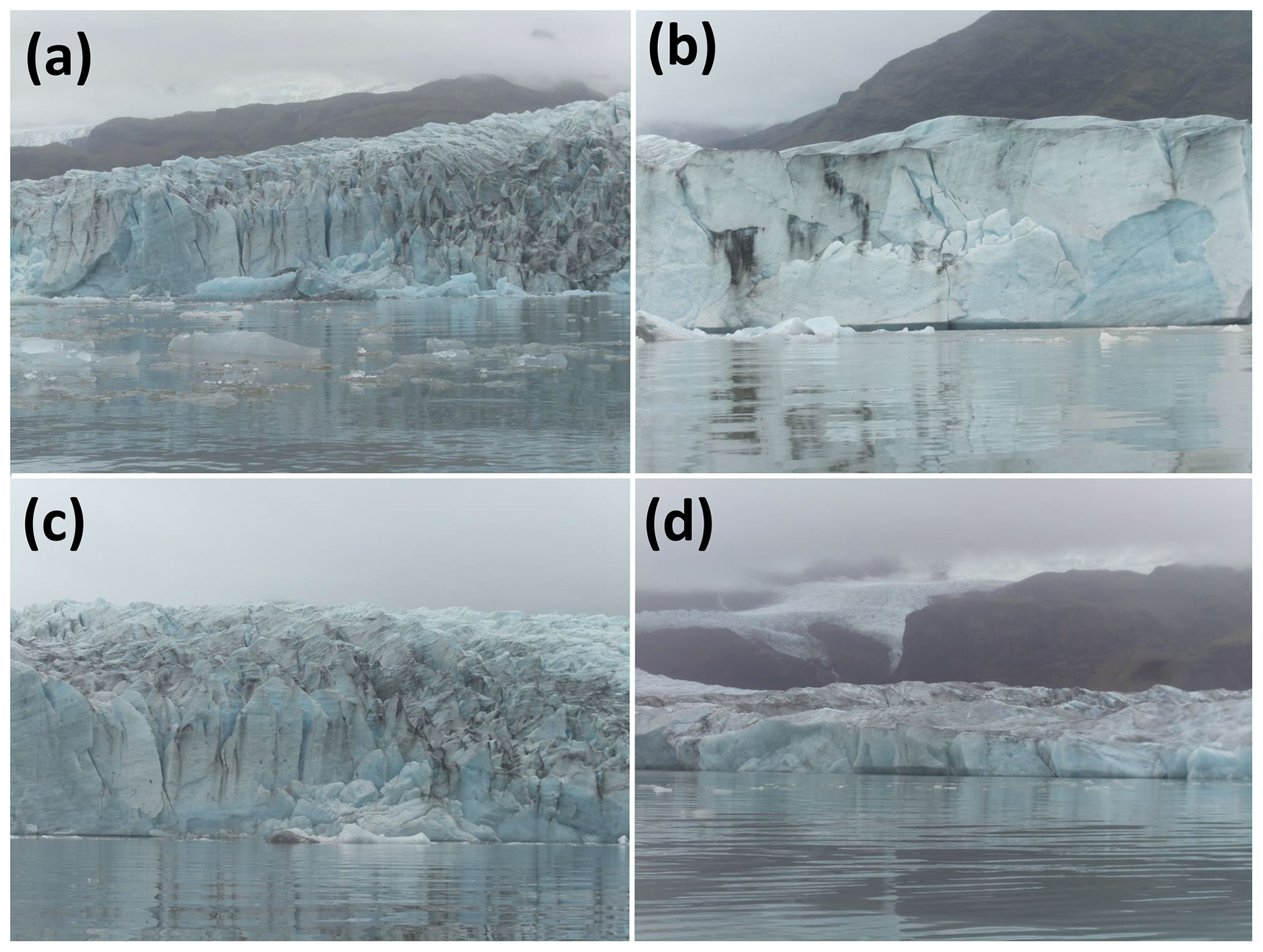
Figure 3Example images captured by the Raspberry Pi sensor. Images A, B, and C are taken from the boat transect (∼500 m from the glacier front) and have an approximate field of vision of ∼100 m, while D is captured from the shoreline ∼1.2 km from the glacier, with an approximate field of vision of ∼400 m.
3.2 Comparison between Raspberry Pi and UAV point clouds
Point clouds generated by the Raspberry Pi show a close comparison to those derived from the UAV, with a mean absolute error of M3C2 distance of 0.301 m and a standard deviation of 0.738 m across the Fjallsjökull calving face (Table 2, Fig. 4). Point density of all Raspberry Pi point clouds was high (<10 cm average spacing between points), allowing small features on the ice surface to be distinguished from ∼500 m away. Extremely high M3C2 values (a threshold greater than 1 m difference between the UAV and Raspberry Pi) are found at the far edges of the models where fewer frames are used to produce the point clouds, and at the highest parts of the margin (particularly prominent in panel E of Fig. 4). These values account for 5.03 % of points (3.31 % > 1 m; 1.72 % > −1 m), and there is a slight positive skew (the Raspberry Pi is overestimating the range to the glacier) in the error distribution with a mean M3C2 distance of 4.31 cm (Fig. 5). The difference in colouration between point clouds (demonstrated in Fig. 4) is likely due to the Raspberry Pi exposure, saturation, and ISO settings all remaining as “auto” to ensure good quality images across the transect. These settings are all fully adjustable if a camera is placed in a fixed position.
Table 2Key statistics and M3C2 comparison between point clouds generated by the Raspberry Pi and UAV. Frontal sub-sections can be seen in Fig. 1.
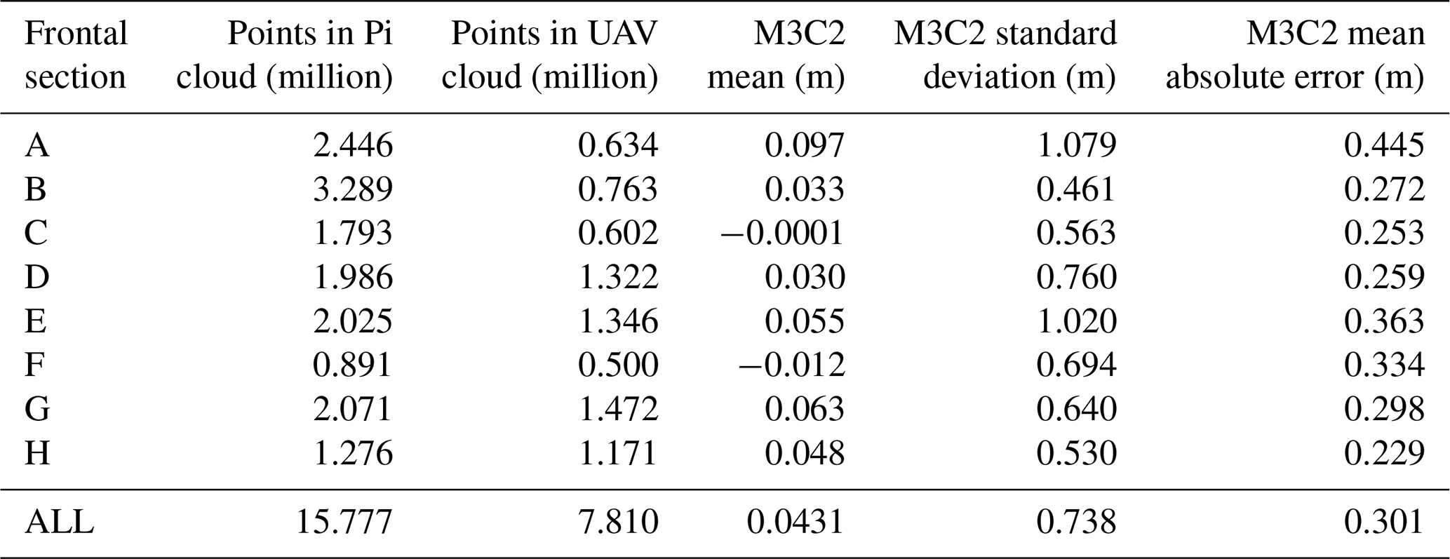
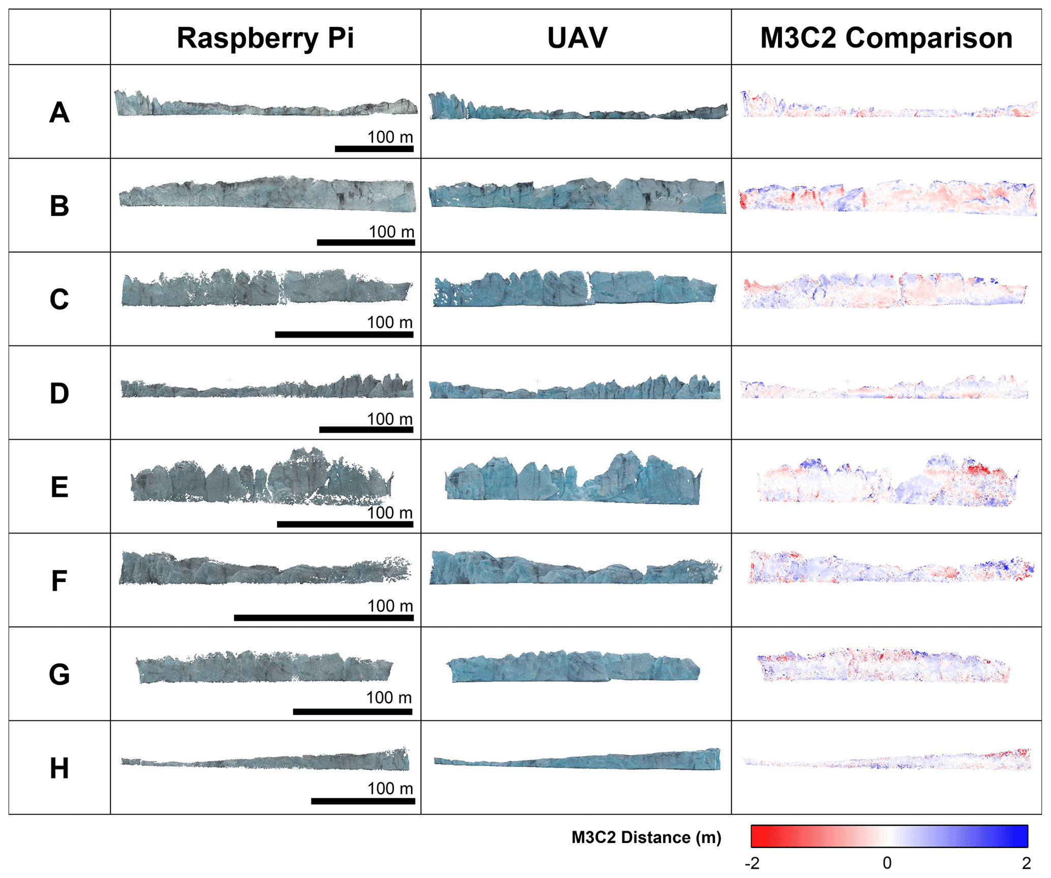
Figure 4Fjallsjökull calving face running from northernmost (A) to southernmost (H) sections, as captured by the Raspberry Pi and UAV, and the M3C2 distance between each. Note varying scales between each section are to minimize white space in figure design.
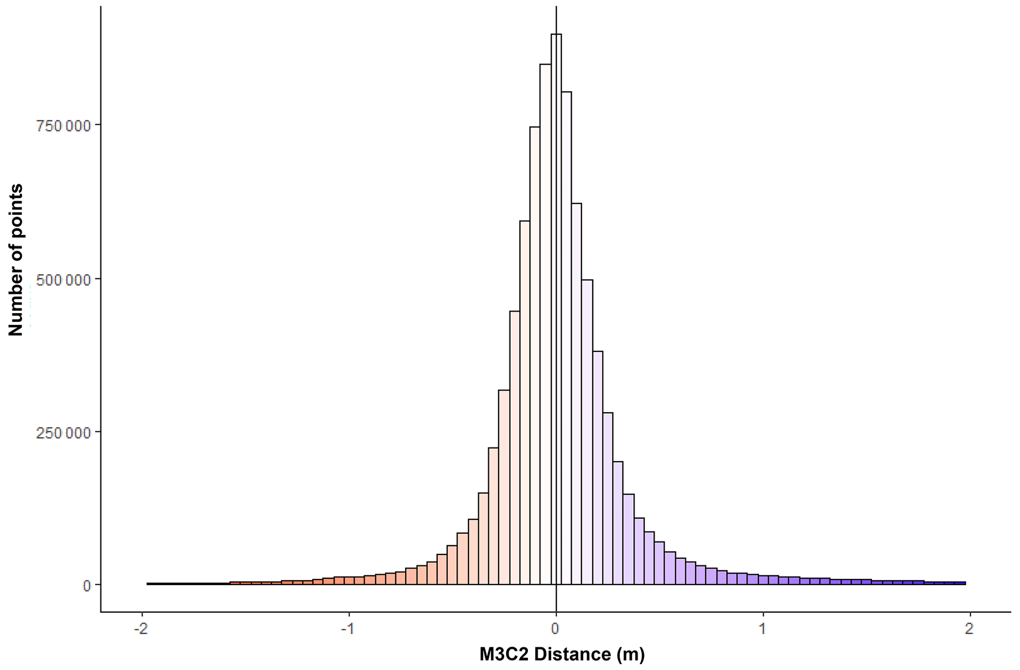
Figure 5Histogram of M3C2 distance values across the Fjallsjökull calving face, combining all eight sub-sections together. There is a slight positive skew in distribution (mean 4.31 cm). M3C2 distances are cropped here to ±2 m for display purposes, but some values reach ±10 m. Bin widths are 0.05 m.
3.3 Exploring the limits of Raspberry Pi cameras in producing 3D models
We analysed sub-section B (∼250 m long) under a number of other scenarios to explore the limits of Raspberry Pi cameras in SfM studies. Capturing images from the shoreline of Fjallsárlón, between 1.2 and 1.5 km away from the calving face (denoted by X and Y in Fig. 1), increased the standard deviation of M3C2 distance (0.742 m compared to 0.461 from the boat transect, a 61 % increase) and mean absolute error (0.341 m compared to 0.272 m from the boat transect, a 25 % increase). The point cloud itself was largely complete, though visibly more speckled than the point cloud generated from the closer survey (Fig. 6). We observed similar patterns of error in the point clouds captured from the shoreline as from the boat transect, with the highest errors corresponding to ridges of jagged ice.
Sub-section B was generated using 31 images from the Raspberry Pi in Fig. 4 and Table 2, but time-lapse camera arrays are generally limited to 10–15 cameras due to cost. We found that using a reduced set of 10 images had little impact on mean absolute error (0.263 m compared to 0.272 m using all images, a 3 % decrease), but increased the standard deviation (0.627 m compared to 0.461 m when using all images, a 36 % increase). This was most notable towards the periphery of the point cloud (Fig. 6G), though the point cloud contains more gaps than the original. Sub-section B is approximately 250 m long and an individual image captures ∼80 m of the glacier front, which means there was a low level of overlap (2–3 images at the right hand side, which is most speckled (Fig. 6). Given the good quality of images acquired at a greater distance, positioning cameras further away to create more overlap between images would likely address this speckle issue.
4.1 Raspberry Pis in SfM-based glaciology studies
Raspberry Pi cameras have rarely been tested in a glaciological setting, but our analysis suggests that they could feasibly be deployed for long-term monitoring purposes and, given their comparable quality to a UAV-derived point cloud, have the potential to capture and quantify dynamic events (e.g. calving). Our data show that, from up to 1.5 km away, Raspberry Pi cameras can detect small features within the ice and, when used to generated 3D data, could identify, with confidence, any displacement of ice over ∼1 m in size. This also holds true for a camera setup using a much-reduced array; our experiments using just 10 camera positions yielded results that were largely comparable in quality to those comprising the full-suite of data (31 camera positions).
Improvements to research design, such as positioning cameras at a more optimal range of heights and angles, including above the glacier, are likely to reduce error in the Raspberry Pi point clouds (James and Robson, 2012; Bemis et al., 2014; Medrzycka et al., 2016; Holmes et al., 2021). A key limitation of our research was that images were captured only from a fixed height in the boat. Indeed, it is no coincidence that we observed the lowest errors between the two sensors at approximately the height level of the boat across all point clouds generated. We also speculate that systematic patterns of error, where high positive error neighbours high negative error such as in Fig. 6e, are due to varying angles of the glacier front being captured in the UAV model but not in the Raspberry Pi which only acquired front-facing images. Therefore, using a greater variety of camera angles and positions, for example by positioning cameras above the glacier front using nearby bedrock or moraines, would likely reduce error across the model (Mosbrucker et al., 2017; Medrzycka et al., 2016; Holmes et al., 2021). While our setup and analysis therefore may represent a conservative view of the potential use of Raspberry Pis in photogrammetry, it also reflects the practical considerations of working in field environments, which are frequently sub-optimal for deploying fixed cameras.
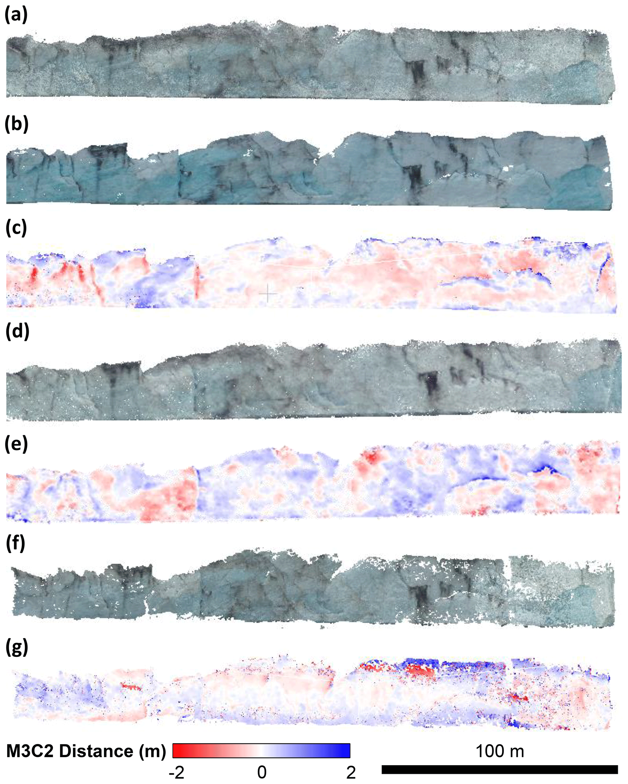
Figure 6Exploring the limits of the Raspberry Pi sensor in comparison to UAV. (a–c) Sub-section B as generated by (a) Raspberry Pi), (b) UAV, and (c) the corresponding M3C2 comparison. (d) Point cloud generated by Raspberry Pi when positioned from the Fjallsárlón shoreline, at a distance of 1.2–1.5 km, and (e) corresponding M3C2 comparison with UAV. (f) Point cloud generated by Raspberry Pi from 10 images, and (g) corresponding M3C2 comparison with UAV.
Our study used relative georeferencing methods, removing the need for absolute positioning of the clouds using surveyed ground control points. Over glacier calving margins, placing ground control points is especially challenging and alternate methods are required (Mallalieu et al., 2017). For example, there is precedent in using the geospatial data from one point cloud to reference another when comparing sensors (Zhang et al., 2019; Luetzenburg et al., 2021). Alternatively, the positions of the cameras can be used to determine the georeferencing. This “direct georeferencing” can be achieved using GNSS-based aerial triangulation of fixed positions, or an on-board GPS unit that shares the clock of the camera such that a precise time-stamp of location can be associated with each of the acquired images (Chudley et al., 2019). Using this approach would allow comparison between repeat point clouds captured by the Raspberry Pi without any alignment to a UAV-based point cloud. For broader photogrammetry applications of the Raspberry Pi, particularly involving setups with only one camera, control points may be essential in capturing the camera position accurately (Schwalbe and Maas, 2017).
In this study, we cropped our point clouds to show only the front, flat, calving face of Fjallsjökull. This involved significant trimming of point clouds generated by the UAV (up to 40 % of points removed), while the Raspberry Pi only required minor adjustments (∼10 % of points removed). A key limitation of the Raspberry Pi setup in our study design is that it cannot achieve the wide range of viewing angles and heights as a UAV does, and so analysis is limited to the front (i.e. vertical section) of the calving face. While this means the setup can monitor advance/retreat and calving events, the additional ability to generate a 3D model of the top of a glacier surface could potentially provide important information on calving dynamics, such as crevasse formation and propagation, which could be indicative of imminent calving (Benn et al., 2007). In previous work, monitoring the glacier surface in addition to the calving face has enabled the reconstruction of events leading up to major calving events, including the calculation of strain rate and identification of propagation prior to calving (Jouvet et al., 2017). Furthermore, other glacier characteristics, such as surface velocity, can indicate imminent calving but require a more top-down view of the glacier surface (Ryan et al., 2015). Modelling a greater extent of the glacier terminus could be particularly important if such a system was to be integrated into a GLOF early warning system.
For studies making use of a typical DSLR-grade handheld camera, James and Robson (2012) and Smith et al. (2016) suggest a typical relative precision ratio of 1:1000 – an error of 1 m when captured at a distance of 1000 m (though high-quality SfM often far exceeds this; James et al., 2017). At 500 m distance, we achieved a mean absolute precision of 1:1667 and at 1.2–1.5 km distance a mean of 1:978. These values almost match the precision thresholds set for DSLR-grade cameras and exceed the precision achieved by similarly priced trail cameras using in glacierized environments (Mallalieu et al., 2017). While terrestrial laser scanners can achieve greater levels of precision for monitoring glacier fronts (e.g. Pętlicki et al., 2015), their high weight and cost (tens of thousands of dollars) often precludes their use in glaciology research.
4.2 Future applications in glaciology and potential for automation
Glacier dynamics at a calving margin are complex, but a low-cost time-lapse camera array can offer insight into many key questions. Ice velocities at the terminus of Fjallsjökull range from ∼40 to ∼200 m a−1 for lake terminating ice (Dell et al., 2019). Glacier frontal positions and their diurnal variability can be monitored using this Raspberry Pi approach, as well as calving events that exceed 1 m in depth. Calving dynamics, including characterizing different types of calving and the impact of seasonality and lake drainage, can also be monitored from time-lapse cameras (Mallalieu et al., 2020) to aid in the understanding of how glacier calving contributes to the overall mass balance of a glacier and how this fluctuates over varying timescales (How et al., 2019; Bunce et al., 2021). Using time-lapse photogrammetry, it is theoretically possible to detect precursors (rotation, elevation change, creep) to calving events on the order of magnitude of >1 m, such as observed at Sermeq Kujalleq 65 h prior to calving (Xie et al., 2016).
In addition to calving events, terrestrial-based photogrammetry based on a Raspberry Pi system could monitor other important glacier dynamics at a low cost. There is a long history of using terrestrial photogrammetry for monitoring glacier thinning to quantify mass balance change of mountain glaciers, though this typically involves repeat site visits (Brecher and Thompson, 1993; Piermattei et al., 2015). Where surrounding topography allows, positioning Raspberry Pi cameras to look down on to the glacier surface would allow for SfM-based velocity calculation (Lewińska et al., 2021). Creep rates of rock glaciers have been successfully monitored through terrestrial photogrammetry (Kaufmann, 2012) and UAV surveys (Vivero and Lambiel, 2019), but again requiring repeated site visits. In each of these additional applications, low-cost Raspberry Pi cameras could produce accurate 3D models at a greater temporal frequency, without the logistical challenges, and financial costs, associated with repeating fieldwork.
Our boat-based study provides confidence that terrestrial-based, high cadence setups could produce regular, accurate 3D models. While not reported in these results, this author team have also successfully operated a separate Raspberry Pi camera in the Peruvian Andes, acquiring three images per day for 3 months using a timer switch and solar panel (Taylor, 2022). Given the customizability of Raspberry Pi cameras, their built-in connectivity, accuracy of acquiring 3D models, and robustness in cold environments, we are confident that arrays of fixed Raspberry Pi cameras could produce the first near real-time photogrammetry setup for continuous 3D monitoring of glacier calving fronts. Outside of photogrammetry, the programmability of Raspberry Pis as terrestrial cameras could offer advances in a broad range of settings, including GLOF management (Mulsow et al., 2015), supraglacial lake drainage (Danielson and Sharp, 2013), and iceberg tracking (Kienholz et al., 2019).
We speculate that, given likely sensor innovation and the decreasing cost of technology, the potential of low-cost sensors in glaciology research will only increase (Taylor et al., 2021). We envisage Raspberry Pi computers, or other microprocessors, to play a key role in this expansion. Almost all Raspberry Pi models have built-in WiFi, which allows data sharing between individual devices. With a WiFi radio on-site, providing a range of many hundreds of metres, individual cameras could autonomously send their data towards a central, more powerful Raspberry Pi unit for further analysis. Similar wireless sensor networks in glaciology have been produced to monitor seismicity (Anandakrishnan et al., 2022), ice surface temperatures (Singh et al., 2018), and subglacial hydrology (Prior-Jones et al., 2021). With the development of autonomous photogrammetry pipelines (Eastwood et al., 2019), a Raspberry Pi-based camera array system could, theoretically, run entirely independent of user input. Furthermore, the flexibility of Raspberry Pi computers, particularly their ability to operate multiple sensor types from one unit, opens up the possibility for wide sensor networks across glaciers – creating comprehensive digital monitoring of rapidly changing environments (Hart and Martinez, 2006; Taylor et al., 2021).
There exists considerable potential for low-cost sensors in mountain glacier communities, which are predominantly located in developing countries. Early warning systems situated around glacial lakes in the Himalaya have successfully prevented disaster during a number of GLOF events by allowing time for downstream communities to evacuate (Wang et al., 2022). By reducing the cost of camera-based sensors that are frequently used as part of a monitoring system (for example at Kyagar glacier in the Chinese Karakorum; Haemmig et al., 2014), more cameras can be situated to monitor calving rates, velocity, or stability at higher precision and accuracy in 3D. A low cost also means that more community-driven initiatives based on this Raspberry Pi system are viable. Such systems must be co-designed, and ultimately owned by, the communities they serve. Simple systems (such as Raspberry Pis), with components that are easily replaceable and with open access documentation, lowers the technical knowledge required to maintain an early warning system, and so a greater diversity of stakeholders can engage with its maintenance. Previous work has shown that diversity in engagement, and genuine understanding of the social structures on which communities are built, is essential for the success of early warning systems like these (Huggel et al., 2020).
4.3 Practical recommendations
While we suggest that Raspberry Pi cameras offer an alternative to expensive DSLR cameras for time-lapse camera arrays, based on our experiences we note a series of recommendations to future researchers and communities looking to use this approach in their own systems:
-
Camera setup must be carefully considered and adopt best practice set by others (e.g. Mallalieu et al., 2017) with regards to angle, overlap, and positioning.
-
Positioning cameras further away from the target (∼1 km) where possible can capture a wider frame of reference while remaining viable for detecting change of magnitude >1 m, so fewer cameras are needed for an array setup.
-
There is only a narrow window of focus when using the Raspberry Pi 16 mm telephoto lens, particularly over 1 km from the target, and an in-field screen is essential to ensure correct setup.
-
While SfM-generated models can be produced without the use of ground control points, such as presented here, it is advisable to collect these to produce accurate photogrammetric measurements from a Raspberry Pi and to allow for comparison between point clouds.
-
In the absence of an in-field screen, Secure Shell Protocol (SSH)-based access to the Raspberry Pi can allow you to see image acquisitions on a computer screen or smartphone, though leaving wireless connectivity enabled draws more power.
-
Raspberry Pi computers draw very little power when commanded to turn on/off between image acquisitions and can be sustained for many months using a lead-acid battery and small solar panel.
-
While Raspberry Pi cameras are robust and usable in sub-zero temperatures, adequate weatherproofing must be used to ensure that the camera lens does not fog over time.
We conducted a photogrammetric survey along the calving face of Fjallsjökull, Iceland, to compare a SfM point cloud generated using imagery from low-cost Raspberry Pi camera sensors to that derived using imagery captured from a UAV. We successfully produced point clouds along the front of Fjallsjökull, with a mean absolute M3C2 distance between point clouds generated by the two sensors of 30.1 cm and a standard deviation of 73.8 cm. The Raspberry Pi camera also achieved sub-metre error at distances of 1.2–1.5 km from the glacier. This error is comparable to DSLR-grade sensors and highlights the potential for Raspberry Pi cameras to be used more widely in glaciology research and monitoring systems. For certain applications, we suggest, conservatively, that Raspberry Pi sensors are viable for detecting change of magnitude >1 m, such as calving events and terminus advance/retreat. With WiFi capabilities within the Raspberry Pi computer, real-time data transmission could open an avenue for autonomous photogrammetry to enable this system to be used in warning against geomorphic hazards. More generally, their affordability, flexibility, durability, and ease of use makes them well-positioned to rival more expensive time-lapse systems without compromising data accuracy, while also enhancing the potential for autonomy and remote system management.
Datasets are openly available at https://doi.org/10.5281/Zenodo.6786740 (Taylor et al., 2022). A list of components and code to replicate the data acquisition are given in the Supplement.
The supplement related to this article is available online at: https://doi.org/10.5194/nhess-23-329-2023-supplement.
LT co-designed the study, conducted data analysis, and wrote the paper. DQ and MS co-designed the study, supervised data analysis, and edited the paper.
The contact author has declared that none of the authors has any competing interests.
Publisher's note: Copernicus Publications remains neutral with regard to jurisdictional claims in published maps and institutional affiliations.
This research was funded by a NERC Doctoral Training Partnership studentship to LST (NE/L002574/1), with additional support from the Geographical Club Award and Dudley Stamp Memorial Award of the Royal Geographical Society (PRA 15.20), the Mount Everest Foundation (19-13), and the Gilchrist Educational Trust. We are thankful to Hannah Barnett for assistance in the field and Joe Mallalieu for his invaluable advice in project design. We are also grateful to Robert Vanderbeck for supporting us through the challenges of conducting fieldwork during a pandemic.
This research has been supported by the UK Research and Innovation (grant no. NE/L002574/1), with additional support from the Geographical Club Award and Dudley Stamp Memorial Award of the Royal Geographical Society (grant no. PRA 15.20), the Mount Everest Foundation (grant no. 19-13), and the Gilchrist Educational Trust.
This paper was edited by Pascal Haegeli and reviewed by Karen Anderson and Penelope How.
Aggarwal, S., Mishra, P. K., Sumakar, K. V. S., and Chaturvedi, P.: Landslide Monitoring System Implementing IOT Using Video Camera, in: 2018 3rd International Conference for Convergence in Technology (I2CT), 1–4, https://doi.org/10.1109/I2CT.2018.8529424, 2018.
Anandakrishnan, S., Bilén, S. G., Urbina, J. V., Bock, R. G., Burkett, P. G., and Portelli, J. P: The geoPebble System: Design and Implementation of a Wireless Sensor Network of GPS-Enabled Seismic Sensors for the Study of Glaciers and Ice Sheets, Geosci., 12, 17, https://doi.org/10.3390/geosciences12010017, 2022.
Armstrong, L., Lacelle, D., Fraser, R. H., Kokelj, S., and Knudby, A.: Thaw slump activity measured using stationary cameras in time-lapse and Structure-from-Motion photogrammetry, Arctic Sci., 4, 827–845, https://doi.org/10.1139/as-2018-0016, 2018.
Bemis, S. P., Micklethwaite, S., Turner, D., James, M. R., Akciz, S., Thiele, S. T., and Bangash, H. A.: Ground-based and UAV-Based photogrammetry: A multi-scale, high-resolution mapping tool for structural geology and paleoseismology, J. Struct. Geol., 69, 163–178, https://doi.org/10.1016/j.jsg.2014.10.007, 2014.
Benn, D. I., Warren, C. R., and Mottram, R. H.: Calving processes and the dynamics of calving glaciers. Earth-Sci. Rev., 82, 143–179, https://doi.org/10.1016/j.earscirev.2007.02.002, 2007.
Bhardwaj, A., Sam, L., Akanksha, Martín-Torres, F. J., and Kumar, R.: UAVs as remote sensing platform in glaciology: Present applications and future prospects, Remote Sens. Environ., 175, 196–204, https://doi.org/10.1016/j.rse.2015.12.029, 2016.
Blanch, X., Abellan, A., and Guinau, M. Point Cloud Stacking: A Workflow to Enhance 3D Monitoring Capabilities Using Time-Lapse Cameras, Remote Sens., 12, 1240, https://doi.org/10.3390/rs12081240, 2020.
Brecher, H. H. and Thompson, L. G.: Measurement of the retreat of Qori Kalis glacier in the tropical Andes of Peru by terrestrial photogrammetry, Photogramm. Eng. Rem. S., 59, 371–379, 1993.
Bunce, C., Nienow, P., Sole, A., Cowton, T., and Davison, B.: Influence of glacier runoff and near-terminus subglacial hydrology on frontal ablation at a large Greenlandic tidewater glacier, J. Glaciol., 67, 343–352, https://doi.org/10.1017/jog.2020.109, 2021.
Carvallo, R., Llanos, P., Noceti, R., and Casassa, G.: Real-time transmission of time-lapse imagery of glaciers in the southern Andes, in: 2017 First IEEE International Symposium of Geoscience and Remote Sensing (GRSS-CHILE), 1–3, https://doi.org/10.1109/GRSS-CHILE.2017.7996019, 2017.
Chakraborty, S., Das, S., Rai, N., Patra, A., Dhar, A., Sadhu, A., Gautam, B., Verma, P., Singh, A., Sherpa, C., and Karn, L.: Development of UAV Based Glacial Lake Outburst Monitoring System, in: IGARSS 2019–2019 IEEE International Geoscience and Remote Sensing Symposium., 9372–9375, https://doi.org/10.1109/IGARSS.2019.8900454, 2019.
Chandler, B. M. P., Evans, D. J. A., Chandler, S. J. P., Ewertowski, M. W., Lovell, H., Roberts, D. H., Schaefer, M., and Tomczyk, A. M.: The glacial landsystem of Fjallsjökull, Iceland: Spatial and temporal evolution of process-form regimes at an active temperate glacier, Geomorphology, 361, 107192, https://doi.org/10.1016/j.geomorph.2020.107192, 2020.
Chudley, T. R., Christoffersen, P., Doyle, S. H., Abellan, A., and Snooke, N.: High-accuracy UAV photogrammetry of ice sheet dynamics with no ground control, The Cryosphere, 13, 955–968, https://doi.org/10.5194/tc-13-955-2019, 2019.
Danielson, B. and Sharp, M.: Development and application of a time-lapse photograph analysis method to investigate the link between tidewater glacier flow variations and supraglacial lake drainage events, J. Glaciol., 59, 287–302, https://doi.org/10.3189/2013JoG12J108, 2013.
Dell, R., Carr, R., Phillips, E., and Russell, A. J.: Response of glacier flow and structure to proglacial lake development and climate at Fjallsjökull, south-east Iceland, J. Glaciol., 65, 321–336, https://doi.org/10.1017/jog.2019.18, 2019.
Eastwood, J., Sims-Waterhouse, D., Weir, R., Piano, S., and Leach, R.,K.: Autonomous close-range photogrammetry using machine learning, in: Proc. ISMTII2019, Niigata, Japan, 1–6 pp., 2019.
Eastwood, J., Zhang, H., Isa, M., Sims-Waterhouse, D., Leach, R., and Piano, S.: Smart photogrammetry for three-dimensional shape measurement, in: Optics and Photonics for Advanced Dimensional Metrology, SPIE Photonics Europe, 43–52, https://doi.org/10.1117/12.2556462, 2020.
Eltner, A., Kaiser, A., Abellan, A., and Schindewolf, M.: Time lapse structure-from-motion photogrammetry for continuous geomorphic monitoring: Time-lapse photogrammetry for continuous geomorphic monitoring, Earth Surf. Proc. Land., 42, 2240–2253, https://doi.org/10.1002/esp.4178, 2017.
Emmer, A., Merkl, S., and Mergili, M.: Spatiotemporal patterns of high-mountain lakes and related hazards in western Austria, Geomorphology, 246, 602–616, https://doi.org/10.1016/j.geomorph.2015.06.032, 2015.
Esposito, G., Salvini, R., Matano, F., Sacchi, M., Danzi, M., Somma, R., and Troise, C.: Multitemporal monitoring of coastal landslide through SfM-derived point cloud comparison, Photogramm. Rec., 32, 459–479, https://doi.org/10.1111/phor.12218, 2017.
Fallourd, R., Vernier, F., Friedt, J.-M., Martin, G., Trouvé, E., Moreau, L., and Nicolas, J.-M.: Monitoring temperate glacier with high resolution automated digital cameras – Application to the Argentière glacier, ISPRS Commission III Symposium, Paris, France, 19–23 pp., 2010.
Ferdoush, S. and Li, X.: Wireless Sensor Network System Design Using Raspberry Pi and Arduino for Environmental Monitoring Applications, Proc. Comput. Sci., 34, 103–110, https://doi.org/10.1016/j.procs.2014.07.059, 2014.
Fugazza, D., Scaioni, M., Corti, M., D'Agata, C., Azzoni, R. S., Cernuschi, M., Smiraglia, C., and Diolaiuti, G. A.: Combination of UAV and terrestrial photogrammetry to assess rapid glacier evolution and map glacier hazards, Nat. Hazards Earth Syst. Sci., 18, 1055–1071, https://doi.org/10.5194/nhess-18-1055-2018, 2018.
Giordan, D., Allasia, P., Dematteis, N., Dell'Anese, F., Vagliasindi, M., and Motta, E.: A Low-Cost Optical Remote Sensing Application for Glacier Deformation Monitoring in an Alpine Environment, Sensors, 16, 1750, https://doi.org/10.3390/s16101750, 2016.
Giordan, D., Dematteis, N., Allasia, P., and Motta, E.: Classification and kinematics of the Planpincieux Glacier break-offs using photographic time-lapse analysis, J. Glaciol., 1–15, https://doi.org/10.1017/jog.2019.99, 2020.
Haemmig, C., Huss, M., Keusen, H., Hess, J., Wegmüller, U., Ao, Z., and Kulubayi, W.: Hazard assessment of glacial lake outburst floods from Kyagar glacier, Karakoram mountains, China, Ann. Glaciol., 55, 34–44, https://doi.org/10.3189/2014AoG66A001, 2014.
Hart, J. K. and Martinez, K.: Environmental Sensor Networks: A revolution in the earth system science?, Earth-Sci. Rev., 78, 177–191, https://doi.org/10.1016/j.earscirev.2006.05.001, 2006.
Holmes, F. A., Kirchner, N., Prakash, A., Stranne, C., Dijkstra, S., and Jakobsson, M.: Calving at Ryder Glacier, Northern Greenland, JGR Earth Surf., 126, e2020JF005872, https://doi.org/10.1029/2020JF005872, 2021.
How, P., Schild, K. M., Benn, D. I., Noormets, R., Kirchner, N., Luckman, A., Vallot, D., Hulton, N. R. J., and Borstad, C.: Calving controlled by melt-under-cutting: detailed calving styles revealed through time-lapse observations, Ann. Glaciol., 60, 20–31, https://doi.org/10.1017/aog.2018.28, 2019.
How, P., Hulton, N. R. J., Buie, L., and Benn, D. I.: PyTrx: A Python-Based Monoscopic Terrestrial Photogrammetry Toolset for Glaciology, Front Earth Sci., 8, 21, https://doi.org/10.3389/feart.2020.00021, 2020.
Howarth, P. J. and Price, R. J.: The Proglacial Lakes of Breidamerkurjökull and Fjallsjökull, Iceland, Geogr. J., 135, 573, https://doi.org/10.2307/1795105, 1969.
Huggel, C., Cochachin, A., Drenkhan, F., Fluixa-Sanmartin, J., Frey, H., Garcia Hernandez, J., Jurt, C., Muñoz Asmat, R., Price, K., and Vicuña, L.: Glacier Lake 513, Peru: Lessons for early warning service development, WMO Bulletin. 69, 45–52, 2020.
James, M. R. and Robson, S.: Straightforward reconstruction of 3D surfaces and topography with a camera: Accuracy and geoscience application: 3D Surfaces and Topography with a camera, J. Geophys. Res-Earth., 117, F3, https://doi.org/10.1029/2011JF002289, 2012.
James, M. R., Robson, S., and Smith, M.W.: 3-D uncertainty-based topographic change detection with structure-from-motion photogrammetry: precision maps for ground control and directly georeferenced surveys, Earth Surf. Proc. Land., 42, 1769–1788, https://doi.org/10.1002/esp.4125, 2017.
James, T. D., Murray, T., Selmes, N., Scharrer, K., and O'Leary, M.: Buoyant flexure and basal crevassing in dynamic mass loss at Helheim Glacier, Nat. Geosci., 7, 593–596, https://doi.org/10.1038/ngeo2204, 2014.
Jawak, S. D., Kulkarni, K., and Luis, A. J.: A Review on Extraction of Lakes from Remotely Sensed Optical Satellite Data with a Special Focus on Cryospheric Lakes, Adv. Rem. Sens., 04, 196, https://doi.org/10.4236/ars.2015.43016, 2015.
Jouvet, G., Weidmann, Y., Seguinot, J., Funk, M., Abe, T., Sakakibara, D., Seddik, H., and Sugiyama, S.: Initiation of a major calving event on the Bowdoin Glacier captured by UAV photogrammetry, The Cryosphere, 11, 911–921, https://doi.org/10.5194/tc-11-911-2017, 2017.
Kääb, A.: Photogrammetry for early recognition of high mountain hazards: New techniques and applications, Phys. Chem. Earth Pt. B., 25, 765–770, https://doi.org/10.1016/S1464-1909(00)00099-X, 2000.
Kaufmann, V.: The evolution of rock glacier monitoring using terrestrial photogrammetry: the example of Äußeres Hochebenkar rock glacier (Austria), Aust. J. Earth Sci., 105, 63–77, 2012.
Kienholz, C., Amundson, J. M., Motyka, R. J., Jackson, R. H., Mickett, J. B., Sutherland, D. A., Nash, J. D., Winters, D. S., Dryer, W. P., and Truffer, M: Tracking icebergs with time-lapse photography and sparse optical flow, LeConte Bay, Alaska, 2016–2017, J. Glaciol., 65, 195–211, https://doi.org/10.1017/jog.2018.105, 2019.
Kneib, M., Miles, E. S., Buri, P., Fugger, S., McCarthy, M., Shaw, T. E., Chuanxi, Z., Truffer, M., Westoby, M. J., Yang, W., and Pellicciotti, F.: Sub-seasonal variability of supraglacial ice cliff melt rates and associated processes from time-lapse photogrammetry, The Cryosphere, 16, 4701–4725, https://doi.org/10.5194/tc-16-4701-2022, 2022.
Kromer, R., Walton, G., Gray, B., Lato, M., and Group, R.: Development and Optimization of an Automated Fixed-Location Time Lapse Photogrammetric Rock Slope Monitoring System, Remote Sens., 11, 1890, https://doi.org/10.3390/rs11161890, 2019.
Lague, D., Brodu, N., and Leroux, J.: Accurate 3D comparison of complex topography with terrestrial laser scanner: Application to the Rangitikei canyon (N-Z), ISPRS Photogramm, 82, 10–26, https://doi.org/10.1016/j.isprsjprs.2013.04.009, 2013.
Lewińska, P., Głowacki, O., Moskalik, M., and Smith, W.A.P.: Evaluation of structure-from-motion for analysis of small-scale glacier dynamics, Measurement, 168, 108327, https://doi.org/10.1016/j.measurement.2020.108327, 2021.
Luckman, A., Benn, D. I., Cottier, F., Bevan, S., Nilsen, F., and Inall, M.: Calving rates at tidewater glaciers vary strongly with ocean temperature, Nat. Commun., 6, 8566, https://doi.org/10.1038/ncomms9566, 2015.
Luetzenburg, G., Kroon, A., and Bjørk, A. A.: Evaluation of the Apple iPhone 12 Pro LiDAR for an Application in Geosciences, Sci. Rep., 11, 22221, https://doi.org/10.1038/s41598-021-01763-9 , 2021.
Lüthi, M. P. and Vieli, A.: Multi-method observation and analysis of a tsunami caused by glacier calving, The Cryosphere, 10, 995–1002, https://doi.org/10.5194/tc-10-995-2016, 2016.
Mallalieu, J., Carrivick, J. L., Quincey, D. J., Smith, M. W., and James, W. H. M.: An integrated Structure-from-Motion and time-lapse technique for quantifying ice-margin dynamics, J. Glaciol., 63, 937–949, https://doi.org/10.1017/jog.2017.48, 2017.
Mallalieu, J., Carrivick, J. L., Quincey, D. J., and Smith, M. W.: Calving Seasonality Associated With Melt-Undercutting and Lake Ice Cover, Geophys. Res. Lett., 47, e2019GL086561, https://doi.org/10.1029/2019GL086561, 2020.
Marzeion, B., Cogley, J. G., Richter, K., and Parkes, D.: Attribution of global glacier mass loss to anthropogenic and natural causes, Science, 345, 919–921, https://doi.org/10.1126/science.1254702, 2014.
Medrzycka, D., Benn, D. I., Box, J. E., Copland, L., and Balog, J.: Calving behavior at Rink Isbrae, West Greenland, from time-lapse photos, Arct. Antarct. Alp. Res., 48, 263–277, https://doi.org/10.1657/AAAR0015-059, 2016.
Messerli, A. and Grinsted, A.: Image georectification and feature tracking toolbox: ImGRAFT, Geosci. Instrum. Method. Data Syst., 4, 23–34, https://doi.org/10.5194/gi-4-23-2015, 2015.
Micheletti, N., Chandler, J. H., and Lane, S. N.: Investigating the geomorphological potential of freely available and accessible structure-from-motion photogrammetry using a smartphone, Earth Surf. Proc. Land., 40, 473–486, https://doi.org/10.1002/esp.3648, 2015.
Minowa, M., Podolskiy, E. A., Sugiyama, S., Sakakibara, D., and Skvarca, P.: Glacier calving observed with time-lapse imagery and tsunami waves at Glaciar Perito Moreno, Patagonia, J. Glaciol., 64, 362–376, https://doi.org/10.1017/jog.2018.28, 2018.
Mosbrucker, A. R., Major, J. J., Spicer, K. R., and Pitlick, J.: Camera system considerations for geomorphic applications of SfM photogrammetry, Earth Surf. Proc. Land., 42, 969–986, https://doi.org/10.1002/esp.4066, 2017.
Mulsow, C., Koschitzki, R., and Maas, H.-G.: Photogrammetric monitoring of glacier margin lakes, Geomat. Nat. Haz. Risk, 6, 861–879, https://doi.org/10.1080/19475705.2014.939232, 2015.
Nota, E. W., Nijland, W., and de Haas, T.: Improving UAV-SfM time-series accuracy by co-alignment and contributions of ground control or RTK positioning, Int. J. Appl. Earth Obs., 109, 102772, https://doi.org/10.1016/j.jag.2022.102772, 2022.
O'Connor, J., Smith, M., and James, M.R.: Cameras and settings for aerial surveys in the geosciences: optimizing image data, Prog. Phys. Geog., 41, 325–344, https://doi.org/10.1177/0309133317703092, 2017.
Pagnutti, M. A., Ryan, R. E., V, G. J. C., Gold, M. J., Harlan, R., Leggett, E., and Pagnutti, J. F.: Laying the foundation to use Raspberry Pi 3 V2 camera module imagery for scientific and engineering purposes, J. Electron. Imaging, 26, 013014, https://doi.org/10.1117/1.JEI.26.1.013014, 2017.
Pętlicki, M., Ciepły, M., Jania, J. A., Promińska, A., and Kinnard, C.: Calving of a tidewater glacier driven by melting at the waterline, J. Glaciol., 61, 851–863, https://doi.org/10.3189/2015JoG15J062, 2015.
Piermattei, L., Carturan, L., and Guarnieri, A.: Use of terrestrial photogrammetry based on structure-from-motion for mass balance estimation of a small glacier in the Italian alps, Earth Surf. Proc. Land., 40, 1791–1802, https://doi.org/10.1002/esp.3756, 2015.
Piras, M., Grasso, N., and Abdul Jabbar, A.: UAV Photogrammetric solution using a Raspberry Pi camera module and smart devices: tests and results, Int. Arch. Photogramm. Remote Sens. Spatial Inf. Sci., XLII-2/W6, 289–296, https://doi.org/10.5194/isprs-archives-XLII-2-W6-289-2017, 2017.
Prior-Jones, M. R., Bagshaw, E. A., Lees, J., Clare, L., Burrow, S., Werder, M. A., Karlsson, N. B., Dahl-Jensen, D., Chudley, T. R., Christoffersen, P., Wadham, J. L., Doyle, S. H., and Hubbard, B.: Cryoegg: development and field trials of a wireless subglacial probe for deep, fast-moving ice, J. Glaciol., 67, 627–640, https://doi.org/10.1017/jog.2021.16, 2021.
Quincey, D. J., Lucas, R. M., Richardson, S. D., Glasser, N. F., Hambrey, M. J., and Reynolds, J. M.: Optical remote sensing techniques in high-mountain environments: application to glacial hazards, Prog. Phys Geog., 29, 475–505, https://doi.org/10.1191/0309133305pp456ra, 2005.
Rosenau, R., Schwalbe, E., Maas, H.-G., Baessler, M., and Dietrich, R.: Grounding line migration and high-resolution calving dynamics of Jakobshavn Isbræ, West Greenland, JGR: Earth Surf., 118, 382–395, https://doi.org/10.1029/2012JF002515, 2013.
Rounce, D., Watson, C., and McKinney, D.: Identification of Hazard and Risk for Glacial Lakes in the Nepal Himalaya Using Satellite Imagery from 2000–2015, Remote Sens., 9, 654, https://doi.org/10.3390/rs9070654, 2017.
Ryan, J. C., Hubbard, A. L., Box, J. E., Todd, J., Christoffersen, P., Carr, J. R., Holt, T. O., and Snooke, N.: UAV photogrammetry and structure from motion to assess calving dynamics at Store Glacier, a large outlet draining the Greenland ice sheet, The Cryosphere, 9, 1–11, https://doi.org/10.5194/tc-9-1-2015, 2015.
Schomacker, A.: Expansion of ice-marginal lakes at the Vatnajökull ice cap, Iceland, from 1999 to 2009, Geomorphology., 119, 232–236, https://doi.org/10.1016/j.geomorph.2010.03.022, 2010.
Schwalbe, E. and Maas, H.-G.: The determination of high-resolution spatio-temporal glacier motion fields from time-lapse sequences, Earth Surf. Dynam., 5, 861–879, https://doi.org/10.5194/esurf-5-861-2017, 2017.
Shiggins, C. J., Lea, J. M., and Brough, S.: Automated ArcticDEM iceberg detection tool: insights into area and volume distributions, and their potential application to satellite imagery and modelling of glacier–iceberg–ocean systems, The Cryosphere, 17, 15–32, https://doi.org/10.5194/tc-17-15-2023, 2023.
Singh, D. K., Gusain, H. S., Mishra, V., Gupta, N., and Das, R. K.: Automated mapping of snow/ice surface temperature using Landsat-8 data in Beas River basin, India, and validation with wireless sensor network data, Arab. J. Geosci., 11, 136, https://doi.org/10.1007/s12517-018-3497-3, 2018.
Smith, M. W., Carrivick, J. L., and Quincey, D. J.: Structure from motion photogrammetry in physical geography, Prog. Phys. Geog., 40, 247–275, https://doi.org/10.1177/0309133315615805, 2016.
Sulak, D. J., Sutherland, D. A., Enderlin, E. M., Stearns, L. A., and Hamilton, G. S.: Iceberg properties and distributions in three Greenlandic fjords using satellite imagery, Ann. Glaciol., 58, 92–106, https://doi.org/10.1017/aog.2017.5, 2017.
Taylor, L. S.: Using a new generation of remote sensing techniques to monitor Peru's mountain glaciers, PhD Thesis, University of Leeds, uk.bl.ethos.868488, 1–184 pp., 2022.
Taylor, L. S., Quincey, D. J., Smith, M. W., Baumhoer, C. A., McMillan, M., and Mansell, D. T.: Remote sensing of the mountain cryosphere: Current capabilities and future opportunities for research, Prog. Phys. Geog., 45, 931–964, https://doi.org/10.1177/03091333211023690, 2021.
Taylor, L., Quincey, D., and Smith, M.: Dataset for: Evaluation of low-cost Raspberry Pi sensors for photogrammetry of glacier calving fronts, Zenodo [data set], https://doi.org/10.5281/zenodo.6786740, 2022.
Tweed, F. S. and Carrivick, J. L.: Deglaciation and proglacial lakes, Geol. Today, 31, 96–102, https://doi.org/10.1111/gto.12094, 2015.
Veh, G., Korup, O., von Specht, S., Roessner, S., and Walz, A.: Unchanged frequency of moraine-dammed glacial lake outburst floods in the Himalaya, Nat. Clim. Chang., 9, 379–383, https://doi.org/10.1038/s41558-019-0437-5, 2019.
Vivero, S. and Lambiel, C.: Monitoring the crisis of a rock glacier with repeated UAV surveys, Geogr. Helv., 74, 59–69, https://doi.org/10.5194/gh-74-59-2019, 2019.
Wang, W., Zhang, T., Yao, T., and An, B.: Monitoring and early warning system of Cirenmaco glacial lake in the central Himalayas, Int. J. Disast. Risk Re., 73, 102914, https://doi.org/10.1016/j.ijdrr.2022.102914, 2022.
Watson, C. S., Quincey, D. J., Smith, M. W., Carrivick, J. L., Rowan, A. V., and James, M. R.: Quantifying ice cliff evolution with multi-temporal point clouds on the debris-covered Khumbu Glacier, Nepal, J. Glaciol., 63, 823–837, https://doi.org/10.1017/jog.2017.47, 2017.
Westoby, M. J., Dunning, S. A., Woodward, J., Hein, A. S., Marrero, S. M., Winter, K., and Sugden, D. E.: Interannual surface evolution of an Antarctic blue-ice moraine using multi-temporal DEMs, Earth Surf. Dynam., 4, 515–529, https://doi.org/10.5194/esurf-4-515-2016, 2016.
Xie, S., Dixon, T. H., Voytenko, D., Holland, D. M., Holland, D., and Zheng, T.: Precursor motion to iceberg calving at Jakobshavn Isbræ, Greenland, observed with terrestrial radar interferometry, J. Glaciol., 62, 1134–1142, https://doi.org/10.1017/jog.2016.104, 2016.
Zemp, M., Frey, H., Gärtner-Roer, I., Nussbaumer, S. U., Hoelzle, M., Paul, F., Haeberli, W., Denzinger, F., Ahlstrøm, A. P., Anderson, B., Bajracharya, S., Baroni, C., Braun, L. N., Cáceres, B. E., Casassa, G., Cobos, G., Dávila, L. R., Granados, H. D., Demuth, M. N., Espizua, L., Fischer, A., Fujita, K., Gadek, B., Ghazanfar, A., Hagen, J. O., Holmlund, P., Karimi, N., Li, Z., Pelto, M., Pitte, P., Popovnin, V. V., Portocarrero, C. A., Prinz, R., Sangewar, C. V., Severskiy, I., Sigurđsson, O., Soruco, A., Usubaliev, R., and Vincent, C.: Historically unprecedented global glacier decline in the early 21st century, J. Glaciol., 61, 745–762, https://doi.org/10.3189/2015JoG15J017, 2015.
Zhang, H., Aldana-Jague, E., Clapuyt, F., Wilken, F., Vanacker, V., and Van Oost, K.: Evaluating the potential of post-processing kinematic (PPK) georeferencing for UAV-based structure- from-motion (SfM) photogrammetry and surface change detection, Earth Surf. Dynam., 7, 807–827, https://doi.org/10.5194/esurf-7-807-2019, 2019.