the Creative Commons Attribution 4.0 License.
the Creative Commons Attribution 4.0 License.
 | 10 Oct 2023
Seismic background noise levels in the Italian strong-motion network
Simone Francesco Fornasari
Deniz Ertuncay
Giovanni Costa
The Italian strong-motion network monitors the seismic activity in the region, with more than 585 stations with continuous data acquisition. In this study, we determine the background seismic noise characteristics of the network by using the data collected in 2022. We analyse the spatial and temporal characteristics of the background noise. It is found that most of the stations suffer from anthropogenic noises, since the strong-motion network is designed to capture the peak ground motions in populated areas. Hence, human activities enrich the low periods of noise. Therefore, land usage of the area where the stations are located affects the background noise levels. Stations can be noisier during the day, up to 12 dB, and during the weekday, up to 5 dB, in short periods. In long periods (≥ 5 s), accelerometric stations converge to similar noise levels and there are no significant daily or weekly changes. It is found that more than half of the stations exceed the background noise model designed for strong-motion stations in Switzerland by Cauzzi and Clinton (2013) in at least one of the calculated periods. We also develop an accelerometric seismic background noise model for periods between 0.0124 and 100 s for Italy by using the power spectral densities of the network. The model is in agreement with the background noise model developed by D’Alessandro et al. (2021) using broadband data for Italy in short periods, but in long periods there is no correlation among studies.
- Article
(15454 KB) - Full-text XML
-
Supplement
(21361 KB) - BibTeX
- EndNote


Seismic stations record the vibration of the ground that is given by the superposition of multiple sources. The definition of seismic noise varies based on the target of each specific study. Since most of the seismic networks are established to detect seismic events (i.e. earthquakes, volcanic activities, quarry blasts, and nuclear explosions), all other vibrations are referred to as (ambient) noise. On the other hand, ambient noise itself has been the object of specific studies (e.g. for the characterization of layers of the earth, Shapiro et al., 2005; the Moon, Larose et al., 2005; and Mars, Schimmel et al., 2021). Noises can also be sub-categorized based on their source, such as (i) recorders (Ringler and Hutt, 2010), (ii) temperature changes (Stutzmann et al., 2000; Doody et al., 2018), (iii) ocean and sea waves (Webb, 1998; McNamara and Buland, 2004; Bonnefoy-Claudet et al., 2006; Cauzzi and Clinton, 2013; D’Alessandro et al., 2021; Anthony et al., 2022), (iv) gravity-gradient noise (Harms et al., 2009), (v) wind (Mucciarelli et al., 2005; Bonnefoy-Claudet et al., 2006; D’Alessandro et al., 2021; Anthony et al., 2022), and (vi) human activities (McNamara and Buland, 2004; Bonnefoy-Claudet et al., 2006; Cauzzi and Clinton, 2013; Vassallo et al., 2019; D’Alessandro et al., 2021; Anthony et al., 2022) (Fig. 1).
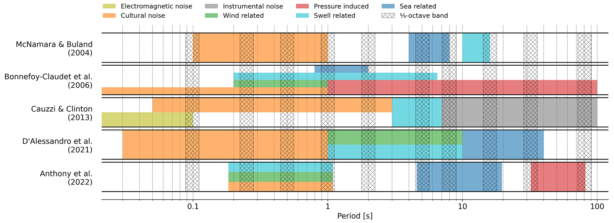
Figure 1Main noise sources at different periods from the studies of McNamara and Buland (2004), Bonnefoy-Claudet et al. (2006), Cauzzi and Clinton (2013), D’Alessandro et al. (2021), and Anthony et al. (2022). The hatched bands represent the one-third-octave bands used for the analysis.
The level of noise affects the quality of the recorded waveforms and hence the ability to detect seismic events. To be able to monitor the seismic sources, seismic networks require knowledge about the noise content of the networks. To characterize the noise at a given station, the frequency content of the noise is calculated via power spectrum density (PSD). The above-mentioned noise sources can be seen in different frequency bands of the PSD (Fig. 1). Various models have been created to interpret the noise levels. The model of Peterson (1993) is widely used to define the lower (new low-noise model, NLNM) and upper (new high-noise model, NHNM) bounds of the recorded noise as a baseline, developed using a worldwide catalogue from a wide variety of seismic stations. Cauzzi and Clinton (2013) developed the accelerometer low-noise (ALNM) and high-noise (AHNM) models using accelerometric data from the Swiss Seismological Service (Clinton et al., 2011) and very broadband data along with accelerometric data from the Southern California Seismic Network (California Institute of Technology and United States Geological Survey Pasadena, 1926). The AHNM is computed as the lower boundary of 5th-percentile PSD amplitudes observed on rock sites in which urban noise, microseismic activities, and data logger systems dominate the short periods, mid-range periods, and long periods, respectively. The ALNM is computed as a particular combination of accelerometric sensors with a given gain and response with data loggers. This model is widely used as the baseline model for strong-motion sensors (Ringler et al., 2015, 2020).
The National Accelerometric Network (RAN), owned and managed by the Italian Civil Protection Department (DPC) (Presidency of Counsil of Ministers – Civil Protection Department, 1972; Gorini et al., 2010; Zambonelli et al., 2011; Costa et al., 2022), was established to monitor strong motions at a national level. The integrated RAN is the combination of the RAN with the following networks: (i) the Friuli Venezia Giulia and Veneto Accelerometric Network (RAF, Rete Accelerometrica Friuli Venezia Giulia in Italian; University of Trieste, 1993; Costa et al., 2010) in north-east Italy, owned and managed by the University of Trieste (UniTS), and (ii) the Irpinia Seismic Network (ISNet; Weber et al., 2007) in the south of Italy, owned and managed by the Analysis and Monitoring of Environmental Risk Society (AMRA). Hereafter, RAN will refer to the integrated RAN. With the RAN main goal being to provide information valuable for civil protection duties, the selection criteria of the “optimal” location to install seismic stations weigh multiple parameters, and the quality of the recordings in terms of noise generated by nearby sources could play a secondary role.
In this paper, we focused on the background noise in the RAN by analysing the data recorded by 585 continuous stations during 2022 and we developed the Italian accelerometric noise models. We focused our analysis mainly on the short periods (≤5 s), since they carry more relevant information related to parameters useful for civil defence purposes (e.g. peak ground acceleration (PGA) and peak spectral acceleration (PSA0.3, PSA1.0, and PSA3.0)). The progressive conversion of data acquisition from triggered to continuous recording starting from the end of 2020 increased the number of stations available to study noise levels on a national scale.
In Sect. 2, we explain the properties of the RAN and the time coverage of the data. In Sect. 3, the data preprocessing, PSD evaluation workflow, and development of the Italian accelerometric noise models are explained. Background noise levels and the noise models are presented in Sect. 4, and the possible noise sources, temporal and spatial variations of the noise, and a comparison between previous background noise models with the developed model are discussed in Sect. 5.
In this study, data from the vertical component of 585 stations of the RAN collected in 2022 have been analysed (Fig. 2). The RAN stations generally have a standardized installation near urban areas (see Table 1) in free-field conditions, with instruments placed on an isolated pillar anchored on rock or put inside of the sediments. On average, 383 of these stations were operational in continuous recording for more than 90 % of the year. We set a threshold of 50 % of completeness of PSD time series for data selection to calculate the background noise model for the RAN, which makes 494 out of 585 stations (84.6 % of stations) eligible for the further steps: the remaining stations either operated in triggered mode throughout the year or converted to continuous data recording later in the year.
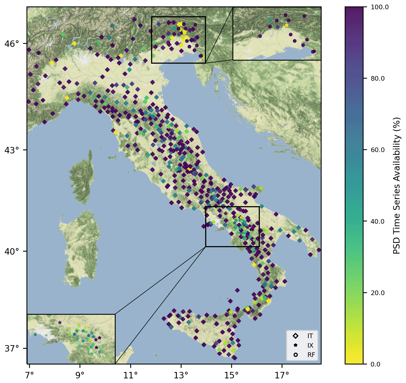
Figure 2PSD time-series availability of the RAN in 2022. The close-up boxes in the lower left and upper right highlight ISNet (IX) and RAF (RF), respectively. Basemap data are retrieved from © Stamen Design.
Table 1Land usage at the RAN stations (Istituto Superiore per la Protezione e la Ricerca Ambientale, 2022).
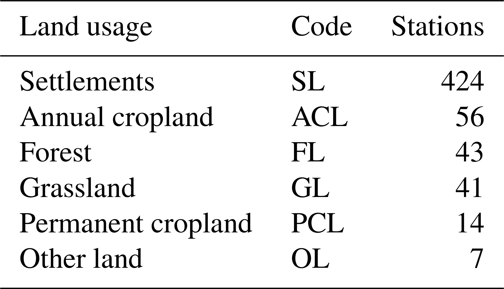
Table 2Sensors at the integrated RAN stations.
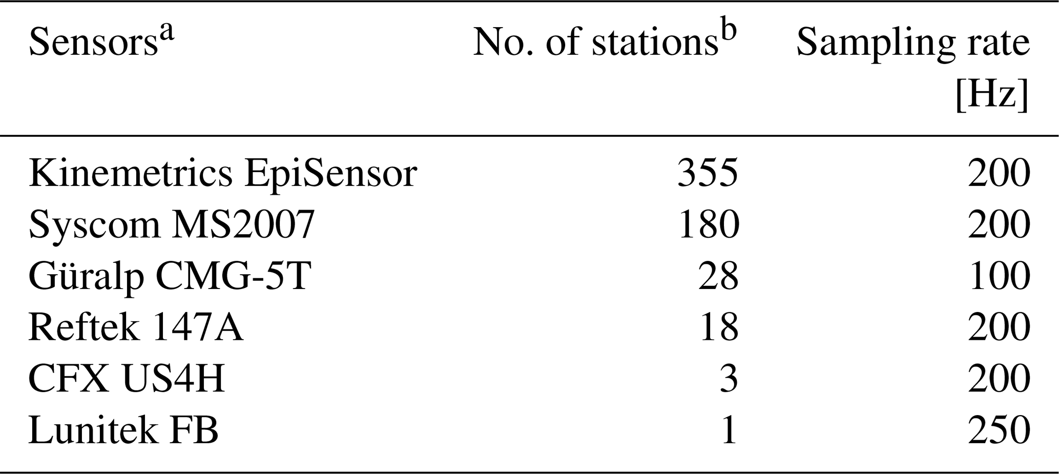
a Equipped with 24-bit recorders. b Status at 1 January 2022.
Seismic instruments of the network consist mostly of Kinemetrics and Syscom sensors (Table 2) with 24-bit acquisition. Data transfer from the station to the data centre in Rome, Italy, is carried out mainly by an access point name (APN) dedicated to the RAN, and a copy of the data is sent to Trieste (Italy) via a virtual private network (VPN).
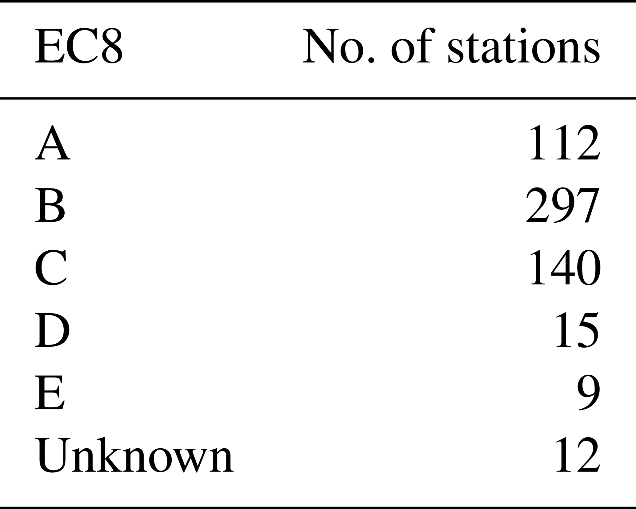
The evolution of the RAN is about not only the combination of several networks but also the installation of new stations across the Italian territory over time. Moreover, the data acquisition systems of the network have changed over time. Since 2020, a large number of triggered stations have been replaced with continuous data acquisition. The purpose of the RAN is to determine the ground motion parameters recorded in the areas where there is considerable human activity. The RAN provides valuable information to the Italian civil defence (DPC) to help in decision-making after seismic events. Because of that, factors that affect the quality of the seismic waveforms recorded (i.e. background noise levels and soil conditions) may not be the main priority for DPC in deciding where a new station is going to be deployed. Most of the RAN stations (Table 3) sit on top of a B and C class soil (Aucun et al., 2012), and many of the stations are located in the settlements (Table 1).
Table 3Soil conditions of the integrated RAN stations (Felicetta et al., 2023).
The method introduced by McNamara and Buland (2004) represents the de facto standard for the evaluation of PSDs. This method was originally developed as a tool for monitoring the status of seismic stations: as such, the original parameters used for the computation of the PSDs and the use of smoothing and averaging provide a way to reduce the storage and computation costs involved but can be limiting when the method is extended to scientific uses, as shown by Anthony et al. (2020).
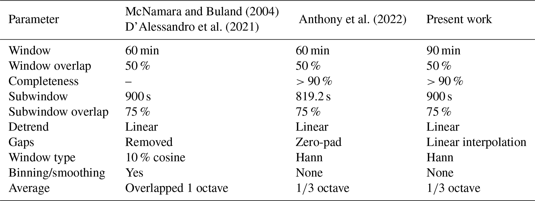
The method implemented to compute the PSDs partially mirrors the one by Anthony et al. (2022), which in turn is an adaptation of McNamara and Buland (2004). Considering only the vertical components at the stations, each daily recording in acceleration is divided into 90 min windows with 50 % overlap, each one subsequently divided into 15 min subwindows with 75 % overlap: as pointed out by Anthony et al. (2020), the window length becomes less relevant for higher frequencies and noisier stations, which are the conditions of the present study. Data completeness above 90 % is required for each 90 min window. Transient signals, consisting also of earthquakes, are not removed from the seismic traces since they are low-probability occurrences with respect to ambient seismic noise (McNamara and Buland, 2004): Anthony et al. (2020) showed that while the presence of earthquakes in the recordings can skew the median ambient noise estimates for longer periods (10–50 s), no significant effects have been observed for short periods. During preprocessing, data are linearly detrended, the gaps are linearly interpolated, and a Hann window is applied to limit spectral leakage (Peterson, 1993; Anthony et al., 2022). For each 15 min subwindow, the PSD is computed using Welch’s method (Welch, 1967), the results for all the subwindows within each 90 min window are averaged, and the instrument response is then removed from the PSD. No binning and smoothing are performed during the PSD computation. Similarly to Anthony et al. (2022), we performed a one-third-octave average over the PSDs: the averaging bandwidth can be assumed to be a reasonable trade-off between the obtained spectral resolution and the accuracy in the broadband noise source characterization in each band. The parameters used for the evaluation of the PSDs in our study, along with the ones used in McNamara and Buland (2004), D’Alessandro et al. (2021), and Anthony et al. (2022), are reported in Table 4.
McNamara and Buland (2004)Anthony et al. (2022)D’Alessandro et al. (2021)Table 4Data processing parameters for the evaluation of the PSDs of our study along with the studies of McNamara and Buland (2004), D’Alessandro et al. (2021), and Anthony et al. (2022).
To study specific patterns in the noise levels over time, the PSDs are studied by grouping them over different time ranges. To study the effects of anthropogenic noise it is a common practice to consider the variations between day (08:00–18:00) and night (20:00–07:00 CET; the time zone applies throughout the paper) and between weekday (Monday–Friday) and weekend (Saturday–Sunday). Similarly, the variations between summer and winter are analysed to check the seasonal variations of the noise levels. Stations with more than 50 % of data for both the summer and winter time periods are selected to analyse seasonal effects. The statistics related to these variations are computed over the daily difference of the medians of each group.
The method explained in the previous section is applied to all the stations in the RAN to create the Italian accelerometric high- (IAHNM) and low-noise (IALNM) models (Fig. 3). Amplitudes for each period are given in the Supplement Table S1 for IAHNM and IALNM. In low periods (≤0.1 s), the median of the RAN is closer to the higher end of the noise model developed by Cauzzi and Clinton (2013). Between ≤0.02 s and ≤0.1 s, IAHNM exceeds the AHNM, and between the periods IAHNM and IALNM cover a large range between −124 and −84 dB. IAHNM is in a downtrend from ≤0.08 s to around 1 s, and it goes upward in the longer periods, whereas IALNM is in a general upward trend. Around 1 s, the median of the RAN exceeds the AHNM, and IAHNM is greater than the AHNM between 0.5 and 3.5 s. The upward trend of background noise can be seen in both models, but in our study such a trend is smoother than the model of Cauzzi and Clinton (2013).
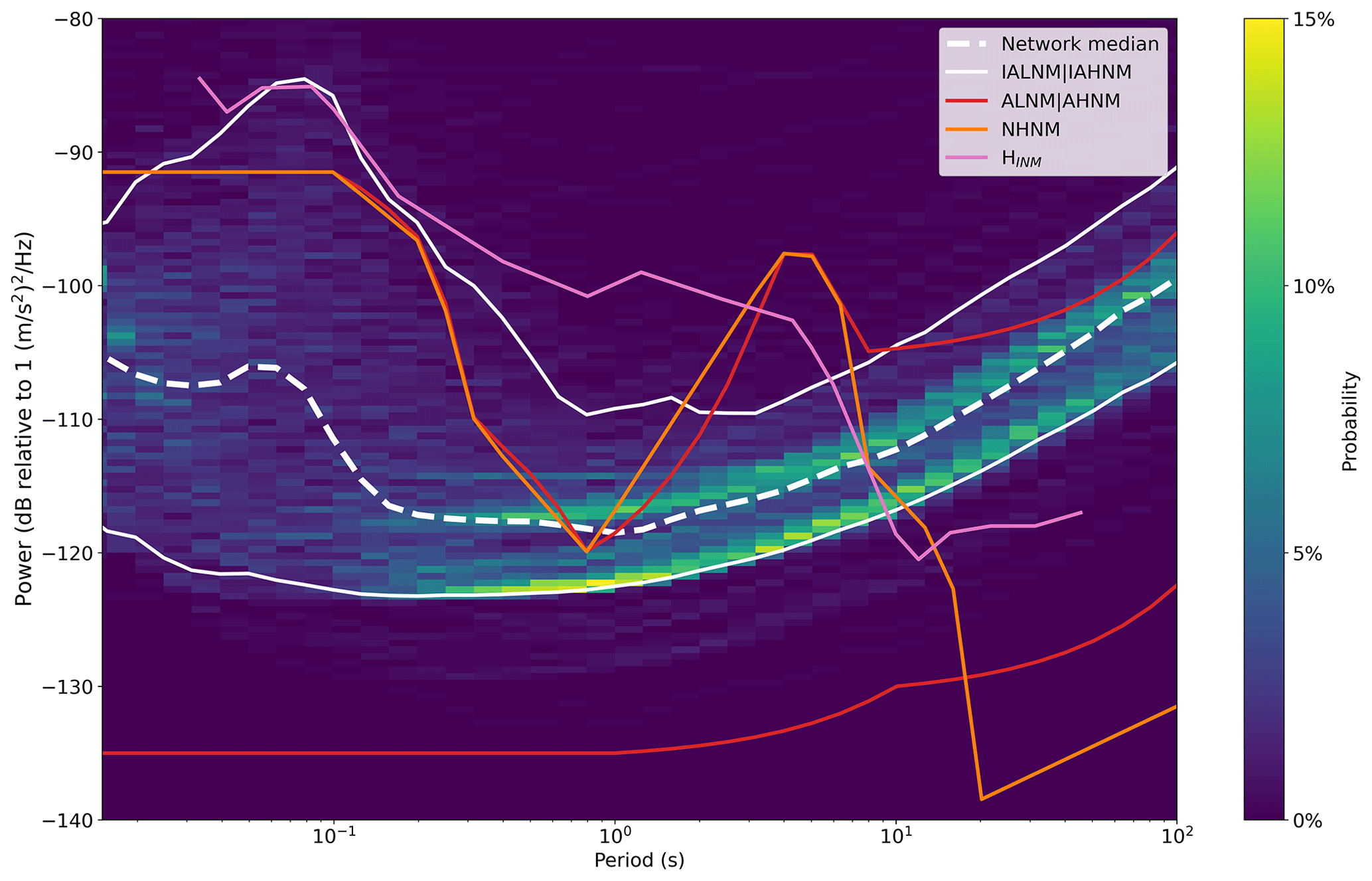
Figure 3PSD probability density function of the RAN. The dashed white line represents the median of the network, and the solid white lines are the 5th-percentile and 95th-percentile limits of the network, IALNM and IAHNM, respectively. The solid red lines represent the ALNM and AHNM defined by Cauzzi and Clinton (2013). The orange and pink lines are NHNM and HINM defined by Peterson (1993) and D’Alessandro et al. (2021), respectively.
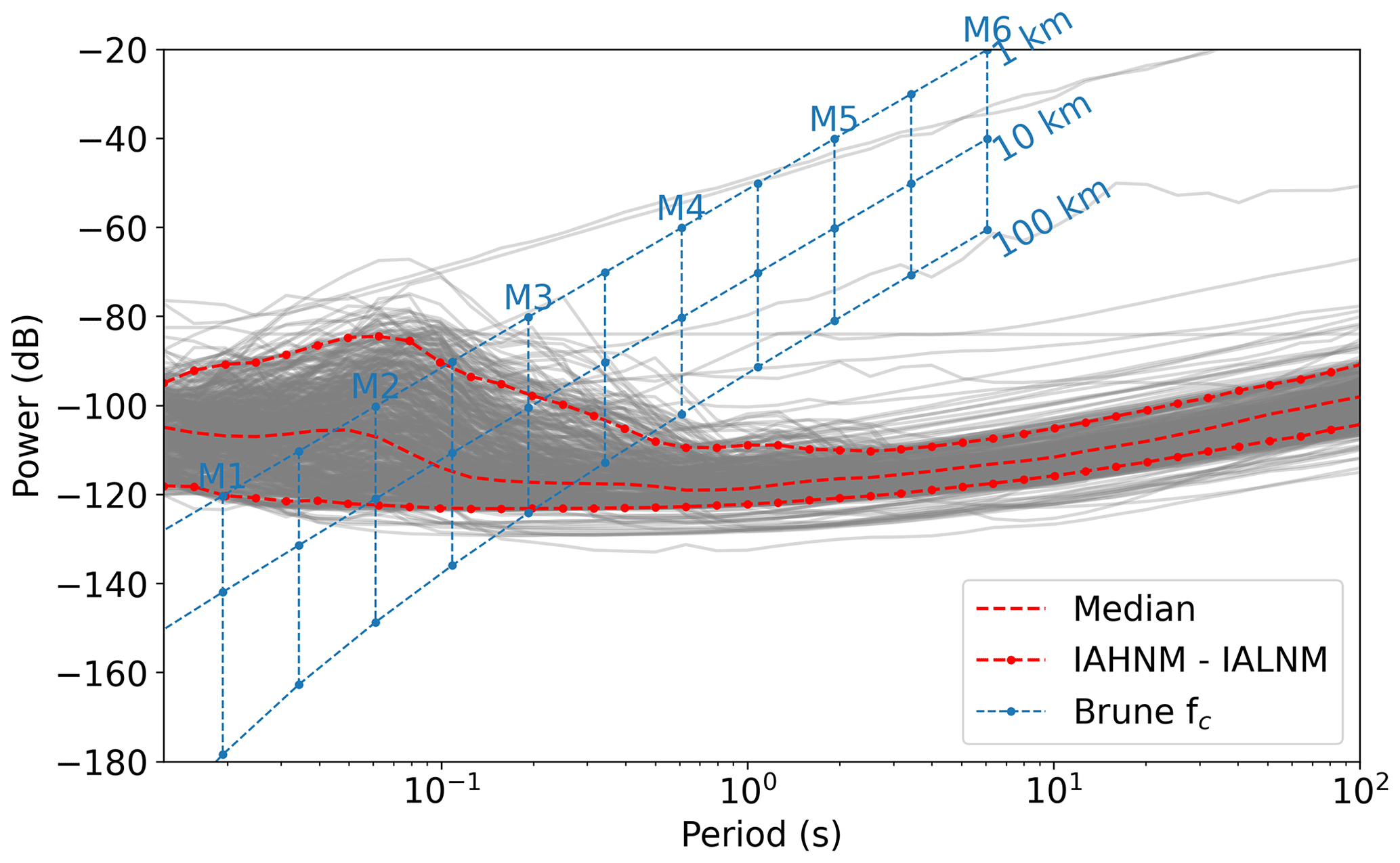
Figure 4Median PSD of the RAN stations (grey lines). The dashed red line and dots represent the median and IAHNM–IAHNM, respectively.
The lower limit of the noise model, IALNM, is, on average, 15 dB higher than the ALNM of Cauzzi and Clinton (2013), which is defined as the theoretical lower boundary of the station noise. Figure 4 shows that only a small number of stations go below the IALNM, and even these stations cannot reach the ALNM model. The PSD values are concentrated in a narrow band in long periods (≥5 s), and in short periods they cover a wide range of values. Station locations play an important role in noise characterization (Fig. 5). Most of the stations that are located in settlements have high levels of noise, hence increasing the upper boundary of the IAHNM. Even though land usage influences short periods, its effect on long periods shows no clear pattern.
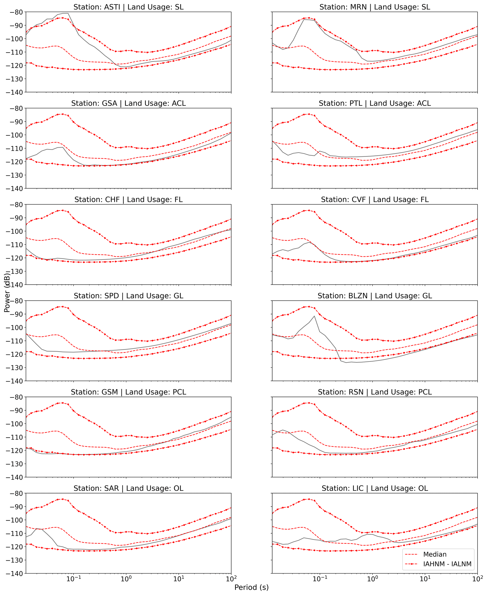
Figure 5Median PSD of two randomly selected stations from each land usage type defined in Table 1. The dashed red line and dots represent the median and IAHNM–IAHNM, respectively.
With the RAN being a strong-motion network, we are mainly interested in periods of less than 5 s; afterwards, we focus on the specific period bands centred around 0.1, 0.25, 0.5, 1, 2, and 5 s. We would like to provide an overview of the behaviour of the noise at different timescales for different periods, as described in detail afterwards (see Fig. 1). The overall background noise levels for all stations in the RAN are presented in Fig. 6. The period-wise median of the PSDs for each station is computed and interpreted as the representative noise level. Anthropogenic sources can have a major role in the noise content of short periods (Fig. 1), which provide essential information for seismic parameters estimation, seismic engineering, and building monitoring. Noise level statistics of the RAN stations for each period of interest are reported in Table S2 with the related noise level and the station placement.
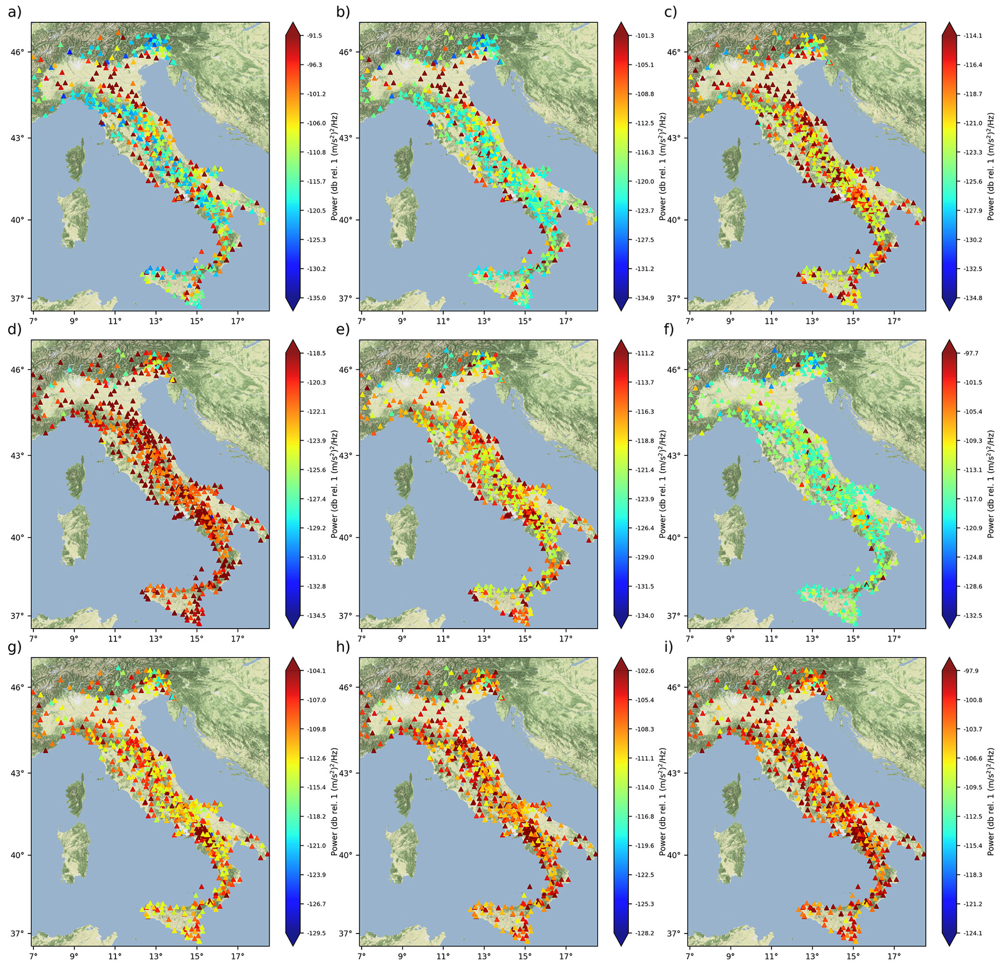
Figure 6Median vertical component noise maps in one-third-octave bands around (a–i) 0.1, 0.25, 0.5, 1.0, 2.0, 5.0, 16.0, 32.0, and 80.6 s. The upper and lower limits of the colour bar are defined by the model developed by Cauzzi and Clinton (2013). The background noise levels of all calculated periods can be found in Fig. S1. The basemap data are retrieved from © Stamen Design.
The RAN has relatively high noise levels in short periods, with numerous stations exceeding the levels defined by Cauzzi and Clinton (2013). The median noise at each station, presented in Fig. 6, and the AHNM have been compared, and the results are reported in Table 5. The period for which we have the highest rate of exceedance of the AHNM level, with 34.4 % of the stations, is 1 s. The probability density function calculated over the median PSD of all stations can be seen in Fig. 3. The median values for 0.1, 0.25, 0.5, 1, 2, and 5 s are −112.59, −119.09, −120.35, −119.98, −118.07, and −115.98 dB, respectively. The median values are always below the AHNM model for the period range of interest. Between 0.1 and 2 s, stations located in the Po Valley and the area from Ischia Island to Naples have relatively high noise levels. Stations around Naples and Ischia Island have the same trend in higher periods.
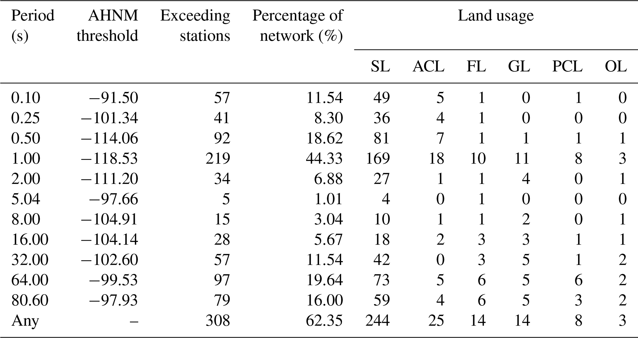
Table 5Number of stations in the network with median noise level exceeding AHNM for different periods.
Under the common assumption that anthropogenic noise decreases during the night hours and the weekend, we characterized the contribution of human activities to ambient noise levels. In 2022, at 493 stations there is a reduction in noise levels at nighttime with respect to the average noise during the daytime (Fig. 7). Daytime–nighttime noise level change reduces with increasing periods at 0.1, 0.25, 0.5, 1, and 2 s with median values of 6.00, 1.45, 0.30, 0.11, and 0.14 dB, respectively. Among these periods, 491, 489, 480, 447, and 439 stations are noisier during the daytime.
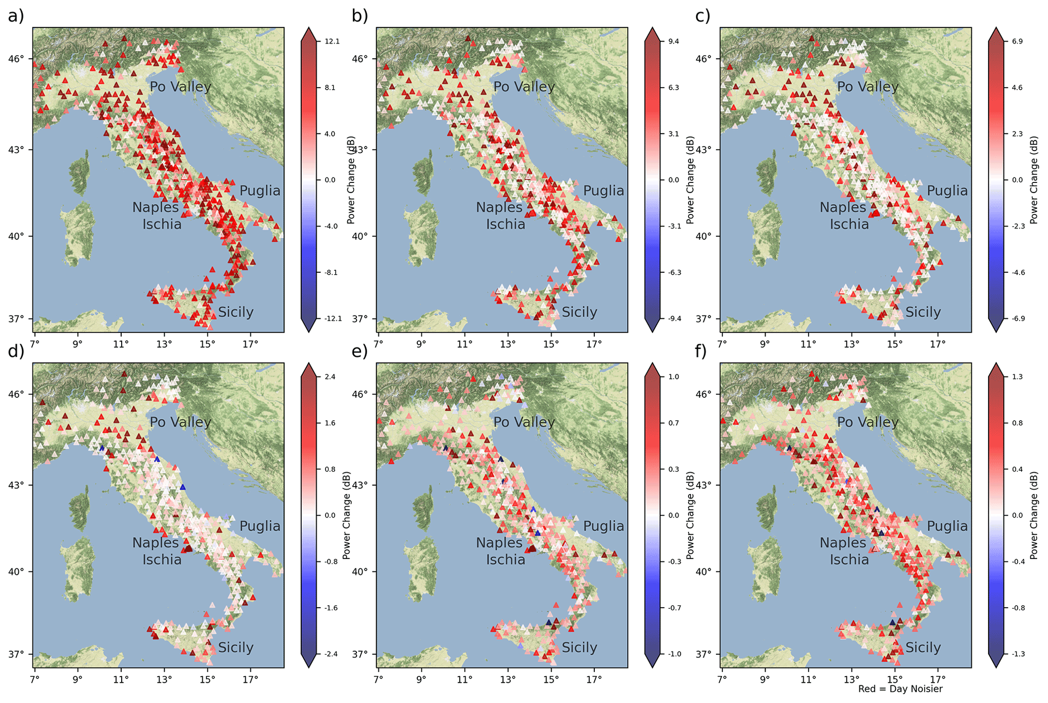
Figure 7The difference between daytime and nighttime for the periods of (a) 0.1 s, (b) 0.25 s, (c) 0.5 s, (d) 1.0 s, (e) 2.0 s, and (f) 5.0 s in decibels (dB). The red colour means day is noisier than night. The basemap data are retrieved from © Stamen Design.
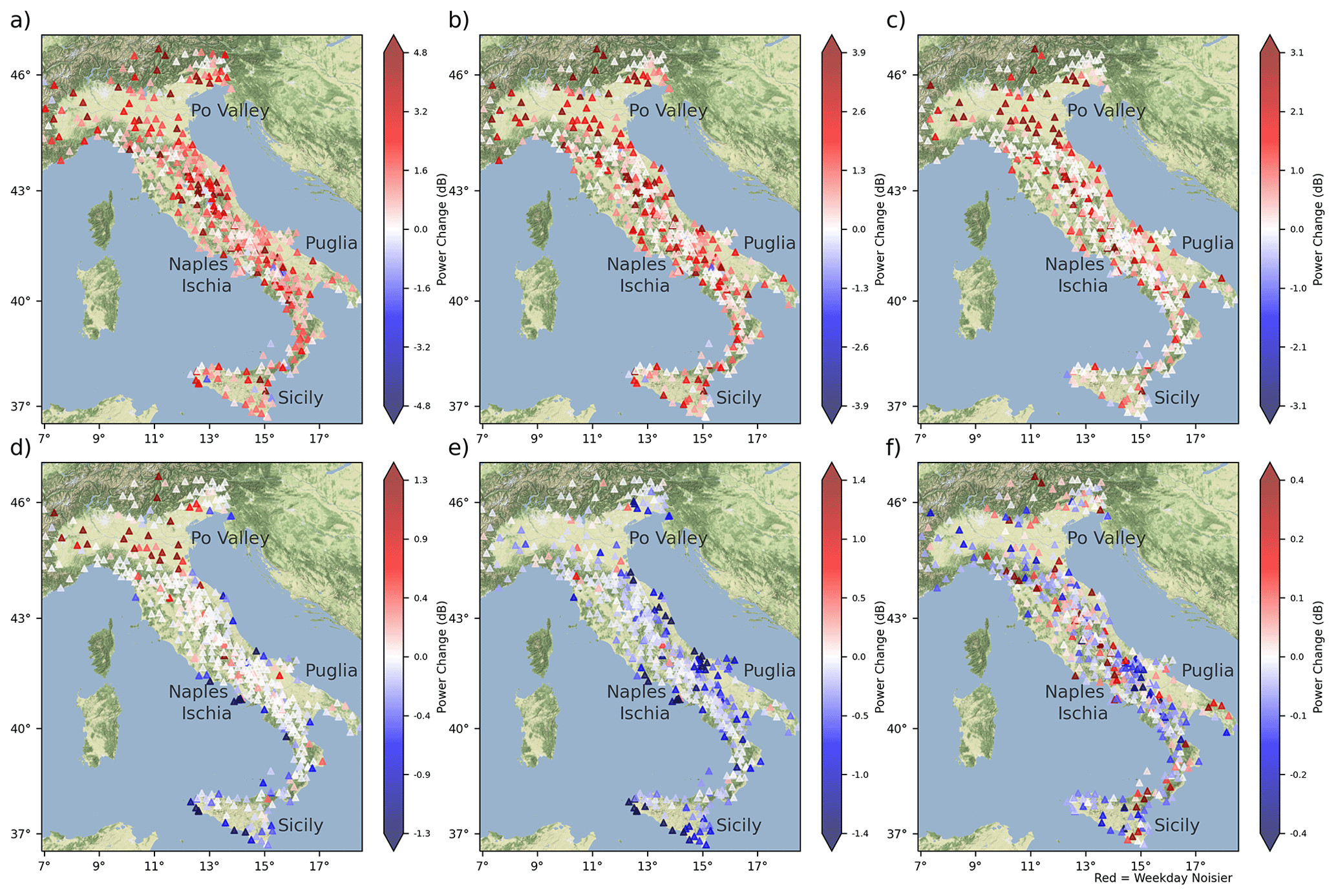
Figure 8The difference between weekday and weekend time for the periods of (a) 0.1 s, (b) 0.25 s, (c) 0.5 s, (d) 1.0 s, (e) 2.0 s, and (f) 5.0 s in decibels (dB). The red colour means weekday is noisier than weekend. The basemap data are retrieved from © Stamen Design.
We also studied the changes in the noise levels between weekdays and weekends, and the general trend of noisier weekdays is observed (Fig. 8) consistently, with the assumption of a reduction in human activities during the weekends. Median changes between weekdays and weekends are smaller with respect to the daytime–nighttime changes, with the same trend of decreasing differences with increasing periods. Weekday–weekend median differences are 0.88, 0.36, 0.08, −0.01, −0.10, and −0.02 dB for 0.1, 0.25, 0.5, 1, 2, and 5 s, respectively. The general trend of noisier weekdays can be followed between 0.1 s and 0.5 s with 453, 453, and 414 stations in the periods of interest. In the periods between 1 s and 5 s, only 215, 52, and 190 stations are noisier on the weekends.
To see the seasonal changes in the long periods which can be affected by the marine and atmospheric sources, we analysed the stations in their median summer and winter (McNamara and Buland, 2004) noise level changes (Fig. 9) by defining 21 June to 21 September as summer and 21 December to 21 March as winter. Surprisingly, in long periods summer time is noisier than the winter time at 5, 8, 16, and 30 s. These periods are chosen to visualize the effect of the long period background noise at the network level. Previous studies (e.g. McNamara and Buland, 2004; Anthony et al., 2022) have found the opposite behaviour in the stations. In total, the median difference between summer and winter are 0.19, 0.97, 1, and 0.75 dB for 5, 8, 16, and 30 s, respectively. The purpose of the accelerometric network is to detect the peak ground parameters in destructive earthquakes. Parameters such as peak ground acceleration (PGA) and peak spectral acceleration (PSA) in short periods provide meaningful information about the possible damage in a site of interest, and these parameters are, in general, observed at the station in the high frequencies of its spectrum. Hence, high background noise levels in long periods do not affect the capabilities of the RAN.
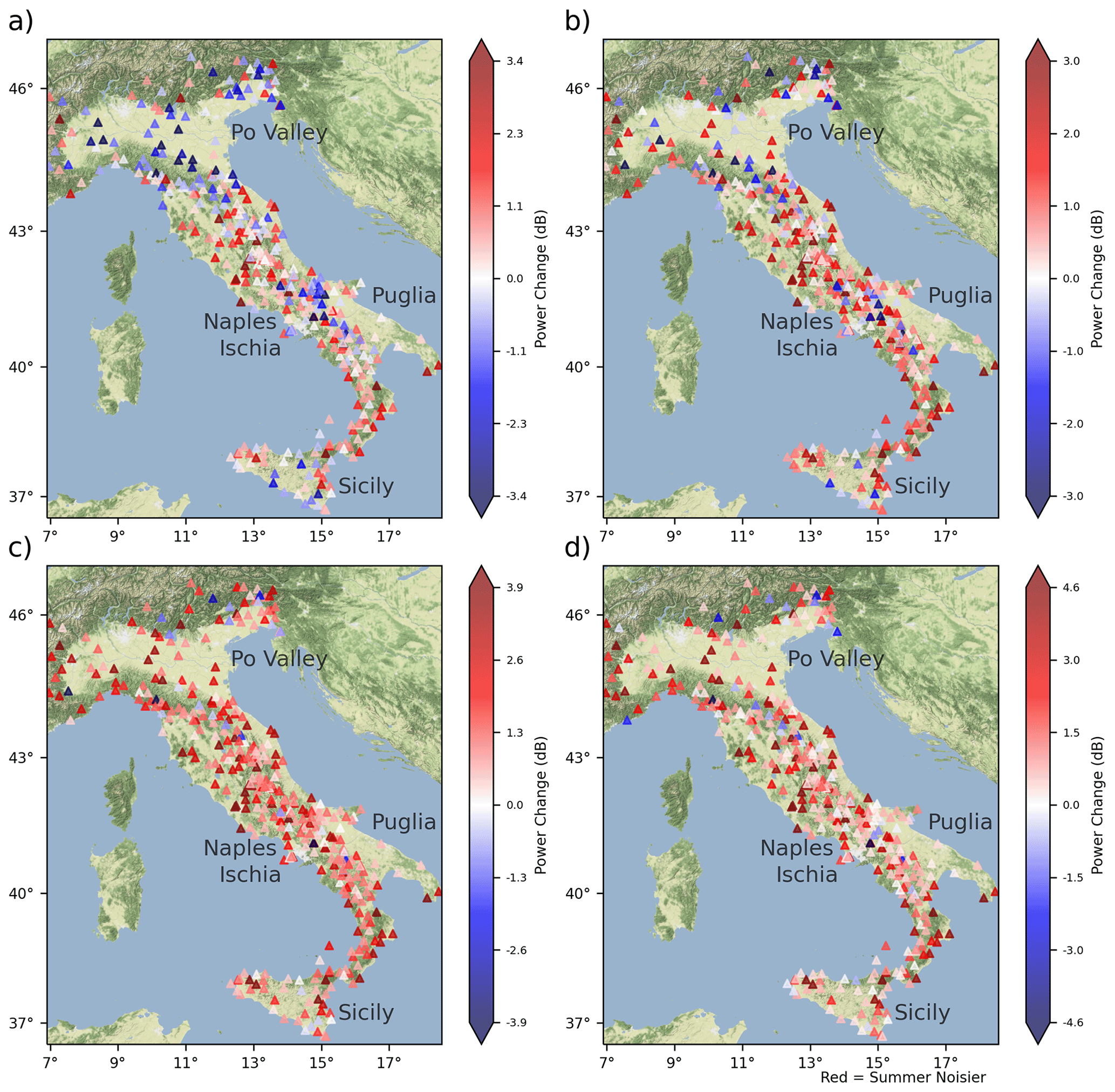
Figure 9Seasonal median noise level change in decibels for (a) 5 s, (b) 8 s, (c) 16 s, and (d) 32 s. The red colour means summer is noisier than winter. The basemap data are retrieved from © Stamen Design.
Table 1 shows the distribution of the stations according to the classification proposed by Istituto Superiore per la Protezione e la Ricerca Ambientale (2022). Even though most of the stations are located in urban areas and potentially subjected to high levels of anthropogenic noise, this classification is too reductive (e.g. not considering the population density and the presence of or making a distinction between residential and industrial areas) to be associated with specific noise levels.
The interpretation of the background noise in the RAN can be done in three different ranges which are low periods (< 1 s), medium-range periods (between 1 and 5 s), and long periods (> 5 s). As mentioned before, in the low periods, human activities are the main source of background noise. A total of 291 of the 493 stations have noise levels exceeding the AHNM developed by Cauzzi and Clinton (2013), as reported in Table 5, considering the results for different periods. In Table 5, the highest percentage of stations exceeding the AHNM is at 1 s. This can be due to the specific data logger systems used by the RAN, as discussed by Cauzzi and Clinton (2013), that shift the background noise levels up and cause network-wide high noise levels (Fig. 6) at this specific period. Furthermore, both the geological and anthropogenic settings of Switzerland present some differences from the Italian ones. Different geodynamic forces act on Italy which create diverse geological structures in the territory, whereas in Switzerland the geology is more homogeneous. The cultural noise is also different between the two countries: the stations used in Cauzzi and Clinton (2013) are, with the exception of the ones in Basel, mainly located in the countryside or in small settlements with respect to the RAN stations.
The potential relation between the geological settings and the background noise characteristics in low periods is also investigated. Stations located in the Po Valley, having large alluvial deposits, have relatively high noise levels (Fig. S2; Cocco et al., 2001). However, there are other noisy stations that are located in completely different geological settings, such as the ones in Naples (local geology is dominated by intrusive rocks). Hence, high background noise cannot be directly linked to the local geology but to the anthropogenic activities. Marzorati and Bindi (2006) analysed the station in and around the Po Valley in terms of background noise by linking the high noise levels to industrial activities and comparing the considerable noise level changes with respect to the stations in the north of the Po Valley. A similar trend can be seen in our results as well (Fig. S2). Stations located in the north-east of the Po Valley (where local geology is dominated by carbonate rocks) are some of the quietest stations in the RAN due to the lack of human activity.
The effect of human activity on noise levels can be seen by comparing daytime noise to nighttime noise, for which human activity is reduced. As seen in Fig. 7, the majority of the stations are noisier during the day for periods less than 1 s. The noise difference between day and night decreases with increasing periods, but the nationwide trend of days being noisier is valid for 0.1, 0.25, and 0.5 s. The same pattern can be seen in broadband stations located in Italy (D’Alessandro et al., 2021). During the daytime, anthropogenic sources (e.g. factories, offices, public buildings, vehicles) may enrich the low-period portion of the background noise. During the nighttime, most of these activities are either reduced or completely stopped. In north-east Italy, there are several stations with a relatively low daytime–nighttime difference. These stations are located far away from all settlements and located in the mountainous parts of Italy. A similar trend can be seen in central Italy at 0.25 and 0.5 s. Le Gonidec et al. (2021) showed that vehicle noises enrich the periods between 0.067 and 0.1 s in seismic signals. At 0.1 s, nationwide daytime–nighttime difference can be linked to vehicles, whereas in periods of 0.25 and 0.5 s other anthropogenic noises (e.g. movement of individuals) can be active. In both north-east and central Italy, these noises can be minimal. Hence, in daytime–nighttime power change there is no significant difference.
In the weekday–weekend variations, the same pattern can be followed in short periods. Figure 8 shows that weekdays were noisier with respect to weekends in almost all stations. The noise level changes are consistent with the changes in weekly human activities. Most of the banks, public buildings, and offices are not working on weekends, and on Sundays commercial activities are reduced, which may limit human activities. Hence, in short periods, the background noise of weekdays is dominated by labour-related activities. As in daytime–nighttime differences, in both north-east and central Italy, there are minimal power change differences, and the same interpretation can be made for the weekday–weekend differences.
In the medium-range periods, there are multiple noise sources that have been identified by previous studies (Fig. 1). Cauzzi and Clinton (2013) stretch the cultural noise up to 3 s, whereas D’Alessandro et al. (2021) indicate that wind- and swell-related noises are dominant between 1 and 10 s. Consequently, variations in the noise sources at 2 and 5 s can be found by analysing the daily, weekly, and seasonal changes.
Day and night differences in medium-range periods follow the trend that is seen in shorter periods except at 1 s. At 1 s, the day and night differences are nulled at most stations, with the notable exception of the stations located in the Po Valley, on Ischia Island, and in Naples, which remain noisier during the day. The majority of the stations exceed the AHNM threshold at 1 s, and the noise levels do not change during the night, which means that the anthropogenic effects are not the dominant source. Even though at 2 and 5 s there is a general trend of having higher noise levels during the daytime, the power change is very small (0.11 and 0.22 dB, respectively). Moreover, the effects of sea, swell, and/or wind at our stations have not been identified and, thus, do not have a significant role in the noise levels: analysing the trend of the median and variability of noise levels at the stations as a function of the distance to the coastline (Fig. S3), no evident pattern emerges, as also shown in Fig. 6. Almost starting from 1 s, background noise levels do not vary too much over the network (Fig. 4), and the effect of sea, swell, and/or wind effect should not significantly alter these forces.
Considering weekly variations, stations become noisier on weekends ≥ 1 s with decreasing power change. In the Po Valley, the general trend of a high noise level diminishes starting from 2 s on average, and in the same periods, unlike the day and night difference, weekends follow the same trend. At 1 s, central Italy has almost the same noise levels between weekdays and weekends, and at both 1 and 2 s several stations in the central Italy and Sicily coastlines become noisier during the weekend. Previous studies suggest the effects of anthropogenic sources and wind- and sea-related activities to be dominant in those periods. As seen in lower periods, human activity increases the weekday noise levels, which makes it irrelevant to the observation. Sea and wind might be the source of the observation if they could be in Fig. 6, since neither wind- nor sea-related noises should be changed between weekdays and weekends. Hence, we do not have a reasonable explanation about the phenomena.
To show the significant effects that the nearby surroundings of a station can have on its noise level, we considered two RAF stations: CARC (latitude: 45.652, longitude: 13.770) and DST2 (latitude: 45.658, longitude: 13.801), located in Trieste (in north-east Italy). Despite their proximity (< 3 km), they have different noise characteristics. The selection of these two particular stations is further supported by the extensive knowledge of their spatial and administrative information. The DST2 station sits on deep flysch deposits (Fig. 10). The CARC station is located on the ground floor of the Palazzo Carciotti, which is located in the city centre of Trieste and was built in the early 19th century. It crosses with one of the main major roads in the city centre, and the building is surrounded by multi-storey residential buildings. Historically, this area was a salina, and the area was filled with a 27 m depth material layer (Fitzko et al., 2007) to cover up the salina to expand the city in the 18th century (Fig. S4).
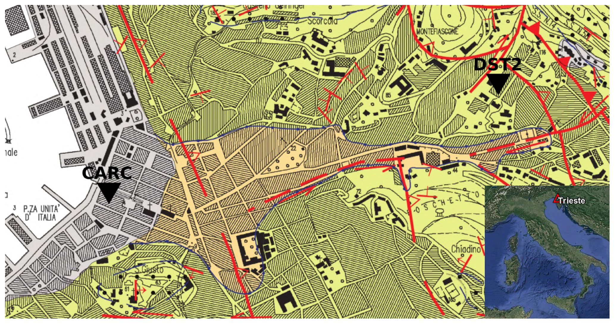
Figure 10Geological map of Trieste (the grey, orange, and yellow colours indicate anthropic deposit units, ubiquitous deposit units, and flysch of Trieste, respectively), modified from Cucchi et al. (2013). The map on the lower right is created by using © Google Earth with satellite information from Landsat/Copernicus.
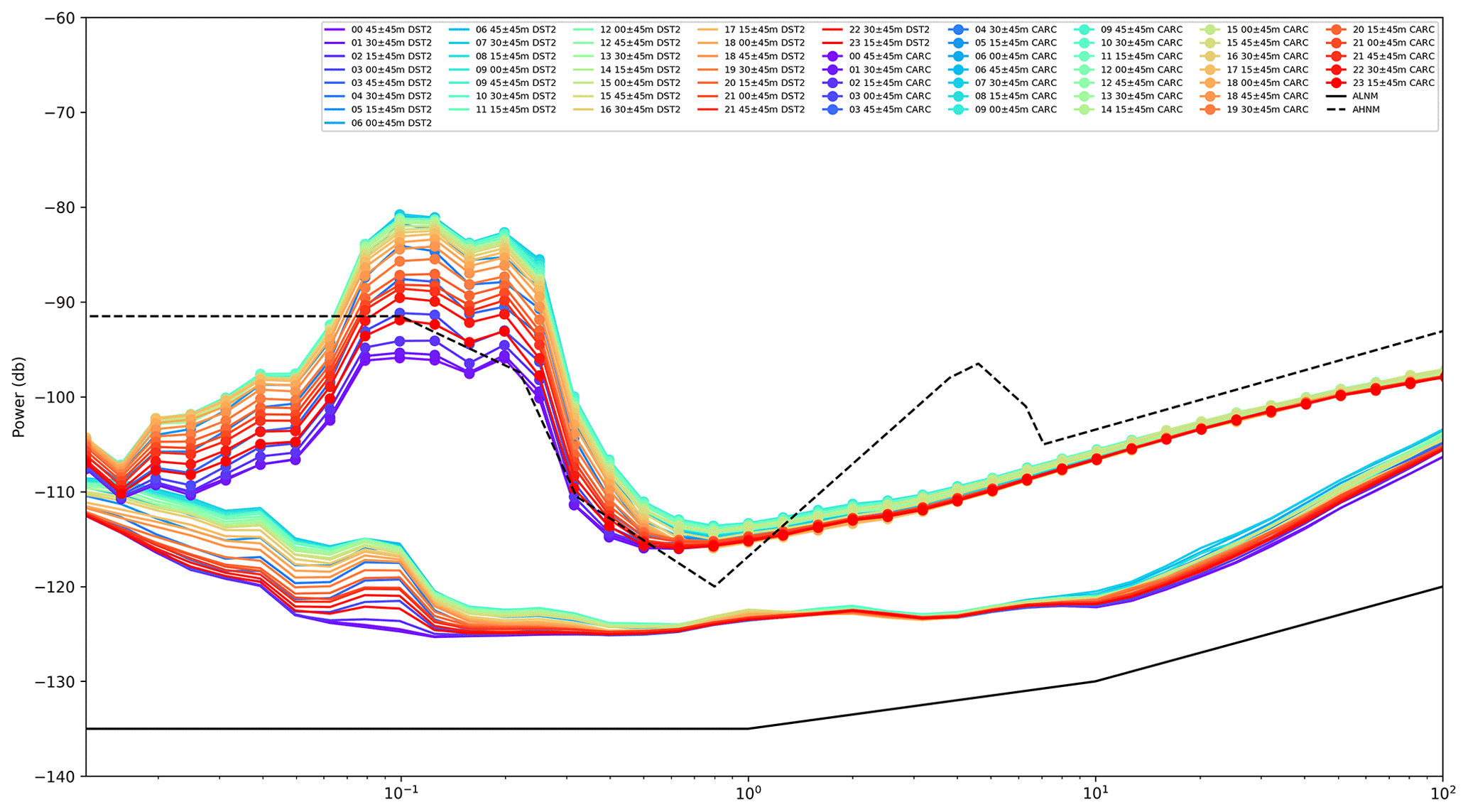
Figure 11Hourly average plots of noise levels of DST2 (line) and CARC (line with dots). The ALNM and AHNM introduced by Cauzzi and Clinton (2013) are the black line and dashed line, respectively.
To see the hourly changes in noise levels, 90 min PSDs are plotted separately (Fig. 11). In the lower periods (< 1 s) where anthropogenic noises prevail, the CARC station is noisier in almost all time ranges. In very short periods (≤ 0.025 s) they converge, but in such low periods electromagnetic noises can be the dominant noise source; hence, background noise can be expected to converge. In the daytime, noise levels of the CARC station converge to the AHNM between 0.2 and 1 s. For periods above 0.5 s, day and night differences are similar, which may suggest that anthropogenic sources do not have a major role. On the other hand, in shorter periods there are clear day–night patterns at both stations. The DST2 station is located in the basement of a small two-storey university building (accommodating just a library, a few offices, and a study room) where human activity is rather limited both inside and outside. Moreover, the building is not located near any major roads. Different environmental factors may play a role in the changing period of the background noise. Both of the stations are located inside buildings; hence, wind effect should be minimal. For periods longer than 10 s, both stations have similar background noise levels and the same trend with increasing periods.
As shown in Table 5, 308 of all the stations exceed the AHNM for at least one period. However, by comparing with the P-wave corner frequencies by Brune (1970), even the 10 noisiest stations theoretically detect the P-wave arrival of a magnitude 2.7 event starting from a 1 km epicentral distance (Fig. S5). Since the purpose of the RAN is to record peak amplitudes, those stations are useful even for earthquakes with smaller magnitudes and longer epicentral distances.
Measuring the background noise levels of the RAN allows us to understand the earthquake detection capability. As presented in Fig. 4, detection of M≈3 earthquakes is possible by near-fault stations in raw signals with the stations near the IAHNM. At median noise level it is possible to detect M≈2 in near-fault stations. The DPC publish M≥2.5 earthquakes in quasi-real time (https://ran.protezionecivile.it/EN/, last access: 2 August 2023). The data filtering algorithm of Gallo et al. (2014) allows us to reduce the background noise to detect ground motion parameters up to 100 km away from the epicentre for M=2.5 earthquakes (Fig. S6). Even though earthquakes with small magnitudes are located by the network, they are not published to the public (Costa et al., 2022).
In Fig. 6, there are some areas that follow the pattern found by D’Alessandro et al. (2021), such as in Naples where noise levels are higher than in the stations that are east of inland Naples. At 1 s only the stations in Naples are in agreement with D’Alessandro et al. (2021), and in our study noise levels are much higher in other parts of Italy. The same trend can be seen in longer periods (> 5 s), in which wind and swell are the dominant noise sources. There are numerous stations located in the Po Valley with high noise levels, even though they are far away from the sea, and several stations located in the Alps in north-west Italy. At 0.1 s, we have noisy stations in the Po Valley, Puglia, and the eastern part of Sicily, where our stations are noisier than the ones analysed in D’Alessandro et al. (2021). However, in short periods our results are in agreement with the study of D’Alessandro et al. (2021) in other parts of Italy. We can conclude that human-made activities dominate the low periods of the noise content, and high noise levels can be linked to the activities that are occurring in the area where anthropogenic sources are present. Reduction in human activity can be seen in Fig. 7, in which almost all stations have lower noise levels at night with respect to their daytime counterparts.
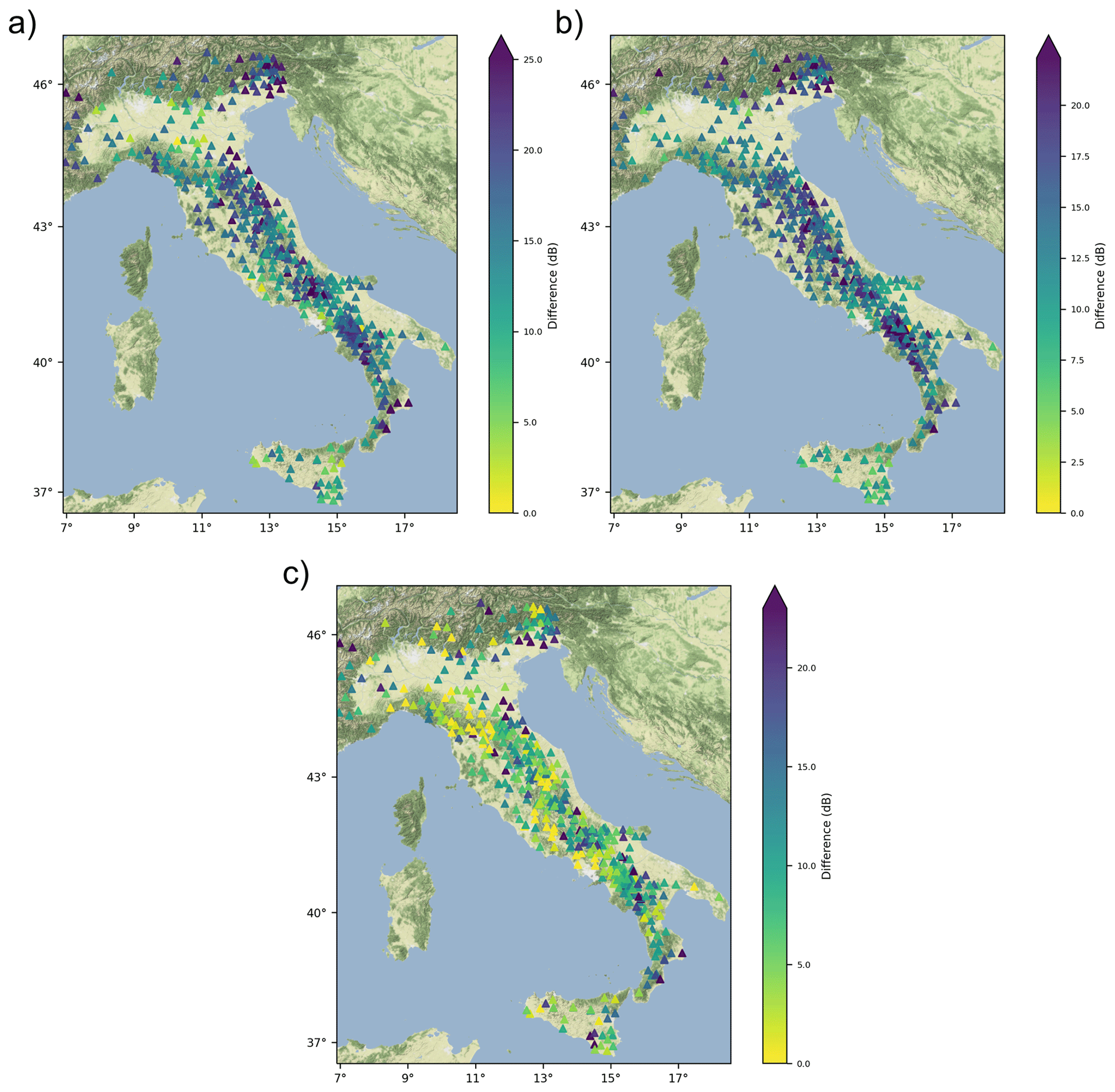
Figure 12Difference between (a) Band II, (b) Band III, and (c) Band IV of D’Alessandro et al. (2021) and our station. Band I is provided in Fig. S7. Basemap data are retrieved from © Stamen Design.
The model by D’Alessandro et al. (2021) has a notable relevance to our study since, first, it covers the same area of interest and, second, spatial variability of their model has been developed by means of the inverse distance weighted method (Lu and Wong, 2008). HINM of the D’Alessandro et al. (2021) study is almost identical to the IAHNM between 0.05 and 0.3 s, which are higher than the AHNM and NHNM of Cauzzi and Clinton (2013) and Peterson (1993). The agreement between the IAHNM in low periods indicates that both broadband and strong-motion networks in Italy get affected by the anthropogenic noises in the same order of magnitude, and in periods between 0.05 and 0.1 s anthropogenic noises have larger effects on the seismic networks with respect to the Swiss and the US seismic networks. Around 1 s, the most significant divergence among the higher limit of the models is observed. The AHNM and NHNM are close to the median of our network, and the IAHNM is about 10 dB higher than them. Interestingly, HINM has even higher noise levels with respect to our model. Between 5 and 10 s, other models converge, whereas our model has a completely different trend. As we discussed before, our model is not susceptible to any long-period trends. The AHNM and IAHNM have similar trends for periods above 10 s, as AHNM was developed by using strong-motion stations.
The second important outcome of the D’Alessandro et al. (2021) study is to model the spatial variance of the noise of the Italian broadband network for four different period bands. This allows us to calculate the predicted noise levels for most of our stations. To compare our noise levels with the predictions of D’Alessandro et al. (2021), we calculate the median of periods that reside in the limits of the bands. The difference between the noise levels in the RAN stations and the model developed by D’Alessandro et al. (2021) can be seen in Fig. 12. In Band IV (0.033 s ≥ T > 0.1 s) of D’Alessandro et al. (2021), anthropogenic sources are the dominant source type, and the major cities of Italy (e.g. Milan, Rome, and Naples) have higher noise levels. In this band, the difference between the background noise of the RAN and the model prediction has greater values in the regions where the model prediction is relatively low, such as north-east Italy and several parts of south Italy. There are numerous stations with almost no difference between the prediction and observation, but there is no overall trend in any geographical location. Since sources of the low-period noises are very local, the difference is mostly dominated by local effects. Hence, there are numerous stations with almost 0 dB difference located near to stations with larger differences in central Italy. In Band III both natural and anthropogenic sources are in action, and the difference between the noise levels in major cities and relatively rural areas of Italy can easily be seen in the model of D’Alessandro et al. (2021).
The recent modernization of the RAN stations allowed us to study their noise levels on a nationwide scale. The analysis is performed by computing PSDs over 90 m windows of signals using continuous recordings acquired in 2022. The results of this study improve the overall seismic background noise information of Italy, complementing the previous work by D’Alessandro et al. (2021) for the Italian broadband network. It is found that a significant number of stations (up to 51.3 % of all stations) have higher noise levels than the AHNM that is defined for accelerometers in Switzerland and California by Cauzzi and Clinton (2013).
As presented in Sect. 4, the RAN has several very noisy stations located within cities. We must stress that the fundamental duty of the RAN is to provide ground motions of the locations where civil defence may need to provide assistance in post-disaster (e.g. strong earthquake) situations. Even though some of these stations are noisy (Table 5), they are well capable of providing the true nature of the ground motion if there is a strong earthquake nearby; hence, they are able to serve their purpose (Costa et al., 2022). Depending on the nature of the future station installations and studies, noise levels of the RAN (Fig. 6) may give an insight into the capabilities of the stations.
The daily variations of the noise levels of the station, obtained by comparing the daytime (08:00–18:00) and nighttime (20:00–07:00) results, show that in short periods where human-made activities dominate the seismic records, daytime is noisier than nighttime. The difference is relatively low in the stations located in the mountainous parts of north-east Italy.
In the longer periods (≥ 1 s), unlike in various previous studies, our analysis has not found any evidence of the swell and sea effect on noise levels (between 1 and 40 s), with no clear pattern arising considering stations at different distances to the coastline (Fig. 6). In periods between 2 and 5 s, winter is noisier, as expected from previous studies (D’Alessandro et al., 2021), but in longer periods it is reversed, and the median noise differences between winter and summer are generally constant network-wise, with the values increasing with periods. These results are consistent with the instrumental noise being the main noise source for long periods, as indicated by Cauzzi and Clinton (2013).
The analysis has been performed using the data and metadata from the Italian strong-motion network (RAN; Gorini et al., 2010; Costa et al., 2022). The data and materials along with the developed models can be found in a dedicated repository: https://github.com/sffornasari/RAN-noise (last access: 29 September 2023; https://doi.org/10.5281/zenodo.8389095, Ertuncay and Fornasari, 2023).
The Supplement contains the maps of the noise levels for each period of interest and a table with the complete comparison between the noise level at the stations and the accelerometric high-noise model (Cauzzi and Clinton, 2013). The supplement related to this article is available online at: https://doi.org/10.5194/nhess-23-3219-2023-supplement.
Conceptualization, all authors; methodology, SFF; software, SFF; data curation, all authors; writing – original draft preparation, DE and SFF; writing – review and editing, all authors; visualization, SFF and DE; supervision, GC; project administration, GC; funding acquisition, GC. All authors have read and agreed to the published version of the paper.
The contact author has declared that none of the authors has any competing interests.
Publisher’s note: Copernicus Publications remains neutral with regard to jurisdictional claims in published maps and institutional affiliations.
This research has been supported by the Dipartimento della Protezione Civile, Presidenza del Consiglio dei Ministri (grant no. RAN2020‐2022 CUP J91F20000110001).
This paper was edited by Oded Katz and reviewed by four anonymous referees.
Anthony, R. E., Ringler, A. T., Wilson, D. C., Bahavar, M., and Koper, K. D.: How processing methodologies can distort and bias power spectral density estimates of seismic background noise, Seismol. Res. Lett., 91, 1694–1706, 2020. a, b, c
Anthony, R. E., Ringler, A. T., and Wilson, D. C.: Seismic background noise levels across the Continental United States from USArray transportable array: The influence of geology and geography, B. Seismol. Soc. Am., 112, 646–668, 2022. a, b, c, d, e, f, g, h, i, j, k
Aucun, B., Fajfar, P., Franchin, P., Carvalho, E., Kreslin, M., Pecker, A., Tsionis, G., Pinto, P., Degee, H., Plumier, A., Fardis, M., Athanasopoulou, A., Bisch, P., and Somja, H.: Eurocode 8 : seismic design of buildings – Worked examples, Publications Office, https://doi.org/10.2788/91658, 2012. a
Bonnefoy-Claudet, S., Cornou, C., Bard, P.-Y., Cotton, F., Moczo, P., Kristek, J., and Fäh, D.: H V ratio: A tool for site effects evaluation. Results from 1-D noise simulations, Geophys. J. Int., 167, 827–837, 2006. a, b, c, d
Brune, J. N.: Tectonic stress and the spectra of seismic shear waves from earthquakes, Journal of Geophysical Research (1896–1977), 75, 4997–5009, https://doi.org/10.1029/JB075i026p04997, 1970. a
California Institute of Technology and United States Geological Survey Pasadena, Southern California Seismic Networks [data set], https://doi.org/10.7914/SN/CI, 1926. a
Cauzzi, C. and Clinton, J.: A high-and low-noise model for high-quality strong-motion accelerometer stations, Earthq. Spectra, 29, 85–102, 2013. a, b, c, d, e, f, g, h, i, j, k, l, m, n, o, p, q, r, s, t
Clinton, J., Cauzzi, C., Fäh, D., Michel, C., Zweifel, P., Olivieri, M., Cua, G., Haslinger, F., and Giardini, D.: The current state of strong motion monitoring in Switzerland, in: Earthquake Data in Engineering Seismology, 219–233, Springer, https://doi.org/10.1007/978-94-007-0152-6_15, 2011. a
Cocco, M., Ardizzoni, F., Azzara, R. M., Dall'Olio, L., Delladio, A., Di Bona, M., Malagnini, L., Margheriti, L., and Nardi, A.: Broadband waveforms and site effects at a borehole seismometer in the Po alluvial basin (Italy), http://hdl.handle.net/2122/1197 (last access: 29 September 2023), 2001. a
Costa, G., Moratto, L., and Suhadolc, P.: The Friuli Venezia Giulia Accelerometric Network: RAF, B. Earthquake Eng., 8, 1141–1157, https://doi.org/10.1007/s10518-009-9157-y, 2010. a
Costa, G., Brondi, P., Cataldi, L., Cirilli, S., Ertuncay, D., Falconer, P., Filippi, L., Fornasari, S. F., Pazzi, V., and Turpaud, P.: Near-Real-Time Strong Motion Acquisition at National Scale and Automatic Analysis, Sensors, 22, 5699, https://doi.org/10.3390/s22155699, 2022. a, b, c, d
Cucchi, F., Piano, C., Fanucci, F., Pugliese, N., Tunis, G., Zini, L., Covelli, S., Fanzutti, G. P., Ponton, M., and Fontana, A.: Carta geologica del Carso Classico, https://arts.units.it/handle/11368/2768388 (last access: 29 September 2023), 2013. a
D’Alessandro, A., Greco, L., Scudero, S., and Lauciani, V.: Spectral characterization and spatiotemporal variability of the background seismic noise in Italy, Earth Space Sci., 8, e2020EA001579, https://doi.org/10.1029/2020EA001579, 2021. a, b, c, d, e, f, g, h, i, j, k, l, m, n, o, p, q, r, s, t, u, v, w, x, y
Doody, C., Ringler, A. T., Anthony, R. E., Wilson, D. C., Holland, A. A., Hutt, C. R., and Sandoval, L. D.: Effects of thermal variability on broadband seismometers: Controlled experiments, observations, and implications, B. Seismol. Soc. Am., 108, 493–502, 2018. a
Ertuncay, D. and Fornasari, S. F.: sffornasari/RAN-noise: RAN Noise codes – v1.0.0 (seismology), Zenodo [code], https://doi.org/10.5281/zenodo.8389095, 2023. a
Felicetta, C., Russo, E., D'Amico, M. C., Sgobba, S., Lanzano, G., Mascandola, C., Pacor, F., and Luzi, L.: ITalian ACcelerometric Archive (ITACA), version 4.0, https://itaca.mi.ingv.it/ItacaNet_40/ (last access: 29 September 2023), 2023. a
Fitzko, F., Costa, G., Delise, A., and Suhadolc, P.: Site effects analyses in the old city center of Trieste (NE Italy) using accelerometric data, J. Earthquake Eng., 11, 33–48, 2007. a
Gallo, A., Costa, G., and Suhadolc, P.: Near real-time automatic moment magnitude estimation, B. Earthquake Eng., 12, 185–202, https://doi.org/10.1007/s10518-013-9565-x, 2014. a
Gorini, A., Nicoletti, M., Marsan, P., Bianconi, R., de Nardis, R., Filippi, L., Marcucci, S., Palma, F., and Zambonelli, E.: The Italian strong motion network, B. Earthq. Eng., 8, 1075–1090, https://doi.org/10.1007/s10518-009-9141-6, 2010. a, b
Harms, J., Sajeva, A., Trancynger, T., DeSalvo, R., Mandic, V., and Collaboration, L. S.: Seismic studies at the Homestake mine in Lead, South Dakota, LIGO document, T0900 112–v1, https://dcc-llo.ligo.org/public/0001/T0900112/001/Homestake.pdf (last access: 29 September 2023), 2009. a
Istituto Superiore per la Protezione e la Ricerca Ambientale: Carta Nazionale di Copertura del Suolo, https://www.isprambiente.gov.it/it/attivita/suolo-e-territorio/suolo/copertura-del-suolo/carta-nazionale-di-copertura-del-suolo (last access: 29 September 2023), 2022. a, b
Larose, E., Khan, A., Nakamura, Y., and Campillo, M.: Lunar subsurface investigated from correlation of seismic noise, Geophys. Res. Lett., 32, L16201, https://doi.org/10.1029/2005GL023518, 2005. a
Le Gonidec, Y., Kergosien, B., Wassermann, J., Jaeggi, D., and Nussbaum, C.: Underground traffic-induced body waves used to quantify seismic attenuation properties of a bimaterial interface nearby a main fault, J. Geophys. Res.-Sol. Ea., 126, e2021JB021759, https://doi.org/10.1029/2021JB021759, 2021. a
Lu, G. Y. and Wong, D. W.: An adaptive inverse-distance weighting spatial interpolation technique, Comput. Geosci., 34, 1044–1055, https://doi.org/10.1016/j.cageo.2007.07.010, 2008. a
Marzorati, S. and Bindi, D.: Ambient noise levels in north central Italy, Geochem. Geophy. Geosy., 7, 9, https://doi.org/10.1029/2006GC001256, 2006. a
McNamara, D. E. and Buland, R. P.: Ambient Noise Levels in the Continental United States, B. Seismol. Soc. Am., 94, 1517–1527, https://doi.org/10.1785/012003001, 2004. a, b, c, d, e, f, g, h, i, j, k
Mucciarelli, M., Gallipoli, M. R., Di Giacomo, D., Di Nota, F., and Nino, E.: The influence of wind on measurements of seismic noise, Geophys. J. Int., 161, 303–308, 2005. a
Peterson, J. R.: Observations and modeling of seismic background noise, Tech. rep., US Geological Survey, http://opg.sscc.ru/attachments/073_ofr93-322.pdf (last access: 29 September 2023), 1993. a, b, c, d
Presidency of Counsil of Ministers – Civil Protection Department: Italian Strong Motion Network, [data set], https://doi.org/10.7914/SN/IT, 1972. a
Ringler, A. and Hutt, C.: Self-noise models of seismic instruments, Seismol. Res. Lett., 81, 972–983, 2010. a
Ringler, A. T., Evans, J. R., and Hutt, C. R.: Self-noise models of five commercial strong-motion accelerometers, Seismol. Res. Lett., 86, 1143–1147, 2015. a
Ringler, A. T., Steim, J., Wilson, D. C., Widmer-Schnidrig, R., and Anthony, R. E.: Improvements in seismic resolution and current limitations in the Global Seismographic Network, Geophys. J. Int., 220, 508–521, 2020. a
Schimmel, M., Stutzmann, E., Lognonné, P., Compaire, N., Davis, P., Drilleau, M., Garcia, R., Kim, D., Knapmeyer-Endrun, B., Lekic, V., Margerin, L., Panning, M., Schmerr, N., Scholz, J. R., Spiga, A., Tauzin, B., and Banerdt, B.: Seismic Noise Autocorrelations on Mars, Earth Space Sci., 8, e2021EA001755, https://doi.org/10.1029/2021EA001755, 2021. a
Shapiro, N. M., Campillo, M., Stehly, L., and Ritzwoller, M. H.: High-resolution surface-wave tomography from ambient seismic noise, Science, 307, 1615–1618, 2005. a
Stutzmann, E., Roult, G., and Astiz, L.: GEOSCOPE Station Noise Levels, B. Seismol. Soc. Am., 90, 690–701, https://doi.org/10.1785/0119990025, 2000. a
University of Trieste: Friuli Venezia Giulia Accelerometric Network, International Federation of Digital Seismograph Networks [data set], https://doi.org/10.7914/SN/RF, 1993. a
Vassallo, M., De Matteis, R., Bobbio, A., Di Giulio, G., Adinolfi, G. M., Cantore, L., Cogliano, R., Fodarella, A., Maresca, R., Pucillo, S., and Riccio, G.: Seismic noise cross-correlation in the urban area of Benevento city (Southern Italy), Geophys. J. Int., 217, 1524–1542, 2019. a
Webb, S. C.: Broadband seismology and noise under the ocean, Rev. Geophys., 36, 105–142, 1998. a
Weber, E., Convertito, V., Iannaccone, G., Zollo, A., Bobbio, A., Cantore, L., Corciulo, M., Crosta, M. D., Elia, L., Martino, C., Romeo, A., and Satriano, C.: An advanced seismic network in the Southern Apennines Italy for seismicity investigations and experimentation with earthquake early warning, Seismol. Res. Lett., 78, 622–634, 2007. a
Welch, P.: The use of fast Fourier transform for the estimation of power spectra: a method based on time averaging over short, modified periodograms, IEEE T. Acoust. Speech, 15, 70–73, 1967. a
Zambonelli, E., de Nardis, R., Filippi, L., Nicoletti, M., and Dolce, M.: Performance of the Italian strong motion network during the 2009, L’Aquila seismic sequence (central Italy), B. Earthq. Eng., 9, 39–65, https://doi.org/10.1007/s10518-010-9218-2, 2011. a