Fluid conduits and shallow-reservoir structure defined by geoelectrical tomography at the Nirano Salse (Italy)

Mud volcanoes are fluid escape structures allowing for surface venting of hydrocarbons (mostly gas but also liquid condensates and oils) and water–sediment slurries. For a better understanding of mud volcano dynamics, the characterization of the fluid dynamics within mud volcano conduits; the presence, extent, and depth of the fluid reservoirs; and the connection among aquifers, conduits, and mud reservoirs play a key role. To this aim, we performed a geoelectrical survey in the Nirano Salse Regional Nature Reserve, located at the edge of the northern Apennines (Fiorano Modenese, Italy), an area characterized by several active mud fluid vents. This study, for the first time, images the resistivity structure of the subsoil along two perpendicular cross sections down to a depth of 250 m. The electrical models show a clear difference between the northern and southern sectors of the area, where the latter hosts the main discontinuities. Shallow reservoirs, where fluid muds accumulate, are spatially associated with the main fault/fracture controlling the migration routes associated with surface venting and converge at depth towards a common clayey horizon. There is no evidence of a shallow mud caldera below the Nirano area. These findings represent a step forward in the comprehension of the Nirano Salse plumbing system and in pinpointing local site hazards, which promotes safer tourist access to the area along restricted routes.

1 Introduction

Mud volcanoes are fluid escape structures allowing for surface venting of hydrocarbons (mostly gas but also liquid condensates and oils) and water–sediment slurries. Their shapes vary in size over different orders of magnitude from centimetres to several hundreds of metres (Manga and Wang, 2015). Mud volcanoes are associated with “mud volcanism” processes (Martinelli and Judd, 2004) that may be quite different, ranging from liquefaction due to sediment overpressure and compaction to leakage from poorly sealed hydrocarbon reservoirs (Kopf, 2002). Worldwide, they are broadly distributed on land and on the sea bottom (Milkov, 2005; Mazzini and Etiope, 2017), especially in contractional areas and fast-subsiding basins. Most mud volcanoes are cold seeps, but some are also present in geothermal areas (Amici et al., 2013). Mud transport mechanisms are a matter of debate, being associated both with mud–dike–sill complexes and with diapirs (Tingay, 2009; Roberts, 2011).

Mud volcanoes are usually associated with quiet and continuous eruptions (Tingay, 2009), but sometimes they explode in dangerous and disruptive events. They are hazardous phenomena, because as of today, it is impossible to define the parameters for modelling the recurrence intervals of the extreme events (Gattuso et al., 2021). Azerbaijan hosts some mud volcanoes where the most violent eruptions worldwide are recorded; the Lökbatan mud volcano, for example, explodes every 3–5 years in spectacular eruptions, which send detritus and breccia rafts into the Caspian Sea (Mazzini et al., 2021; Wang and Manga, 2021). In recent times (2006–2016), the massive eruption of the Indonesian Lusi mud volcano, triggered by the drilling of a borehole, continued for years with peak mudflows of 180 000 m³ d⁻¹ that caused the burial of nearby villages and the displacement of 60 000 people (Mazzini et al., 2007; Tingay, 2015). Some historically recorded explosive events occurred at the Salsa di Montegibbio (Sassuolo, Italy), the largest mud volcano in Italy (Borgatti et al., 2019), and were reported by Pliny the Elder (Naturalis Historia) in Roman times (50 CE) and later (1592–1835) by Biasutti (1907), Govi (1906), and Stöhr (1867). Recently (2014), a sudden massive expulsion of fluids at the Macalube di Aragona mud volcano (Agrigento, Italy) caused the deaths of two children (Gattuso et al., 2021). Mud volcanoes, therefore, represent potential geohazards, especially where these features are located next to populated areas or where they are tourist destinations.

Mud volcanoes are natural hydrocarbon seeps and as such are important indicators in hydrocarbon exploration, where they give indications about the level of hydrocarbon maturity and the presence of structural highs related to mud diapirism (Warren et al., 2011), fault traps, and their spill points (Milkov, 2005; Mazzini and Etiope, 2017). Large mud volcano provinces are also associated with giant hydrocarbon accumulations, and many onshore fields in Europe, the Caribbean, the Caspian Basin, and the Caucasus have been discovered by drilling on natural seeps (Mazzini and Etiope, 2017). In Azerbaijan, mud volcanoes are associated with structural traps and their feeders are rooted in or below the reservoirs, forming an interconnected plumbing system (Planke et al., 2003). The relationships between production from reservoirs and activity in nearby mud volcanoes are also an issue of interest; usually, the decrease in fluid pressure during exploitation causes diminishing mud volcanism processes, but, in some cases, there is no effect whatsoever (Mazzini and Etiope, 2017).

Mud volcanoes also have important meaning in different historical and societal contexts (Giambastiani et al., 2022). Geo-tourists interested in visiting mud volcanoes for the scenery or for recreational mud bathing due to the beneficial properties of mud for the skin are numerous throughout the world (Italy, Colombia, Trinidad, Azerbaijan, Georgia, Turkmenistan, and Indonesia). Mud volcanoes also have a religious significance for Hindus and for Fire Temple worshippers (Ateshgah, near Baku in Azerbaijan), and they have been revered at different times by Zoroastrians, Hindus, and Sikhs (Gamkrelidze et al., 2021). This combination of human activities such as geo-tourism and religious worship, as well as settlements in proximity to mud volcanoes, may lead to situations of risk where the fluid emissions are a geohazard.

In the context of mud volcanoes, fluid emissions are geohazards mostly because they can release violently large amounts of mud and hydrocarbons and may degrade the soil, causing caving and quicksand effects. Furthermore, they might also provoke dissociation of gas hydrates in submarine environments (Mazzini and Etiope, 2017). Explosive eruption of mud volcanoes with methane self-igniting phenomena in Azerbaijan is rather common. Tall mud column ejections up to several tens of metres were observed during the aforementioned eruption at the Macalube di Aragona as well as in the Trinidad Piparo mud volcano, causing serious risks for the people in their proximity (Mazzini and Etiope, 2017). Mud pools with diameters on the order of a few metres, non-existent rims, and depths that can reach 15 m (Giambastiani et al., 2022) may potentially be deadly sinks for people and animals. It is therefore necessary to characterize the fluid dynamics within mud volcano conduits; the presence, extent, and depth of the fluid reservoirs; and the connection among aquifers, conduits, and mud reservoirs. Given that it is difficult to image fluid sources and conduits below a sedimentary cover, geophysical investigations have the potential to greatly contribute to this characterization.

Electromagnetic methods are useful where there is contrast in apparent resistivity due to the presence of mud volcano fluids. Transient electromagnetic (TEM) and the radiomagnetotelluric (RMT) methods were applied by Adrian et al. (2015) at mud volcanoes in Perekishkul (also known as Perekischkjul, Azerbaijan), where they observed resistivity variations at shallow depths (<10 m with RMT) and intermediate depths (150 m with TEM) directly below the surface emissions. Three-dimensional electrical resistivity imaging of mud volcanoes in New Zealand by Zeyen et al. (2011) shows pipe-like structures connected to a deep reservoir; the pipe structures occur along a major strike-slip fault plane, which controls fluid surface venting. Geoelectric methods are often combined with other geophysical and geological investigations. A multidisciplinary approach of shallow seismic, georesistivity, and hydrogeochemical surveys was employed (Rainone et al., 2015) near Pineto (central Italy). The survey results show that the mud reservoirs are not just below the mud volcano but also in a fractured zone at 60 m distance from the vent, suggesting the presence of a high-permeability connection (fracture zone) just below the surface clay deposits.

Several seismic surveys above mud volcanoes have been performed and reported in the literature. Albarello et al. (2012) estimated methane emissions at mud volcanoes in Azerbaijan by measuring the seismic tremor at the surface and identified energy bursts that could be related to bubbling at depth. Evans (2007), using industry-acquired seismic reflection data, well data, and satellite imagery, characterized the geophysical expression of large mud volcanoes (diameter >500 m) in the southern Caspian Basin and was able to identify a sequence of wedge-shaped layers of erupted sediments with regularly interlayered bedding, which could be useful to characterize the temporal time history and recurrence periods of the mud eruptions. Kirkham (2016) also used 3D seismic data to characterize mud volcano geometry and seismic character, timing and distribution, and source regions and depletion zones and to understand the mechanisms behind the formation of conduits and ultimately the geometry of extruded bodies in the Nile Delta. This latter study was particularly effective in identifying seal bypass conduits through which large quantities of mud were extruded to the surface.

Mauri et al. (2018), employing on-land gravimetric surveys at the Lusi mud volcano in Indonesia, have shown that this geophysical methodology is effective in characterizing sediment density variations within the basin and in the mud edifice, which can then be related to the presence of fault-and-fracture systems. A three-dimensional deep electrical tomography survey was also performed at the Lusi mud volcano in Indonesia, by Mazzini et al. (2021), who point out the presence of a fault-and-fracture system just underneath the volcano (Mauri et al., 2018) and image a region where a mix of groundwater, mud breccia, hydrocarbons, and boiling hydrothermal fluids is stored below the subsided area in proximity to the major vent.

Geodetic surveys are also important for mud volcanism characterization. Satellite differential interferometry synthetic aperture radar (DInSAR) has been useful for the detection of pre-eruptive ground deformation in Azerbaijan mud volcanoes by Antonielli et al. (2014), who have shown that inflation (vertical uplift up to 20 cm) and subsidence could be related to the mud flowing in shallow reservoirs.

The objective of our work is to use deep geoelectric tomography surveys at the Nirano Salse Regional Nature Reserve in Italy to characterize the fluid dynamics within mud volcano conduits; the presence, extent, and depth of the fluid reservoirs; and the connection among aquifers, conduits, and mud reservoirs. This is necessary to assess the risk level due to mud-venting geohazards in this natural reserve, which every year is visited by tens of thousands of school students and tourists. This study, for the first time, presents a clear image of the subsoil along two perpendicular cross sections down to a depth of 250 m, imaging structures of which nothing was known before. Furthermore, this geophysical investigation integrates well with already-existing geophysical investigations in the area such as that of Accaino et al. (2007), based on 3D seismic data and 2D geoelectric tomography, and that of Antunes et al. (2022), who used P-wave analysis of drumbeat signals and vertical-to-horizontal seismic amplitude to detect mud movement in the subsoil.

Our study, by imaging low-resistivity subsurface aquifers/reservoirs where high-salinity fluid muds concentrate and the fault-/fracture-controlled migration routes associated with surface venting, represents a step forward in our comprehension of the Nirano Salse plumbing system that had previously only been inferred, based on hydrogeologic data, by Giambastiani et al. (2022).

2 Geological introduction to the area

The Nirano Salse Regional Nature Reserve (Nirano Salse from now on) is located at the edge of the northern Apennines (Fiorano Modenese, Italy), an area that is characterized by several active mud fluid vents.

The Nirano Salse, known since the Roman times, is in a beautiful and scenic landscape of northern Italy. With a surface of approximately 75 000 m², the Nirano Salse is one of the largest mud volcano areas of Italy and Europe, as well as one of the most visited (more than 50 000 visitors each year).

The Nirano Salse is located within a geomorphological bowl (Fig. 1a), which resembles a collapsed caldera. The diameter of the bowl is about 800 m, and the difference in elevation between the bowl's rim and its bottom is about 50–60 m. The structure is almost completely circular except in the SE corner, where a small creek cuts across the rim, and at the SW flank of the circular structure, where it is bordered by two relatively NW–SE-oriented steep ridges. Mud pools and gryphons are located within the caldera-like structure in three major groups: two in the northern part and one in the southern part of the bowl.

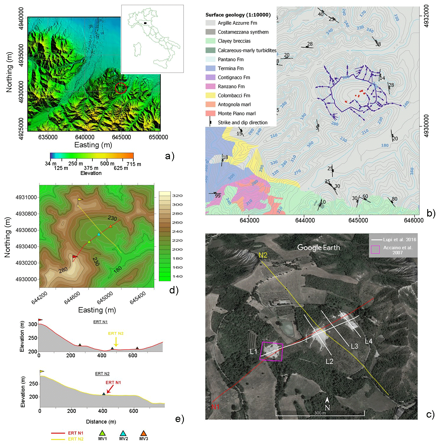
Figure 1 (a) Location of the Nirano Salse area (digital terrain model – DTM – data were downloaded from https://geoportale.regione.emilia-romagna.it/catalogo/dati-cartografici/altimetria/layer-2, last access: 25 July 2023). (b) Surface drainage basin of Nirano, contour lines, and the surface geology modified from the Emilia-Romagna survey geology map, scale 1:10 000 (coordinate reference system: WGS 84/UTM zone 32N). Blue lines with arrows indicate the drainage network in the Nirano area (modified from Giambastiani et al., 2022). (c) Locations of the previous geophysical surveys (© Google Earth 2021). (d) Electrical resistivity tomography (ERT) profile locations on top of a DEM. The red line indicates the position of the ERT_N1 profile. The yellow line indicates the position of the ERT_N2 profile (see text for details). The red and the yellow flags indicate the location of the first electrode on both profiles. Green, cyan, and orange triangles indicate the location of MV1, MV2, and MV3 (see text for details), respectively. (e) Elevation profiles corresponding to ERT_N1 and ERT_N2 profile traces.

There are several individual active cones, gryphons, and subcircular pools distributed at the base of the caldera within an area of recently extruded mud that is free of vegetation. The specific numbers and locations of the cones are rather constant over time, except some small local changes in vent activity. Volcano morphology at the site depends mostly on the characteristics of the extrusion style (abrupt Strombolian-type eruptions forming gryphons), persistence of degassing produced by the rising to the surface of salty and muddy water mixed with gas (mostly CH₄), and connection with groundwater aquifers (mud pools) (Giambastiani et al., 2022).

The Nirano Salse fluid venting occurs in the Plio-Pleistocene Argille Azzurre Fm (FAA for this particular formation; “Fm” denotes “Formation” throughout) (Fig. 1b), which in the southeastern part of the area comprises just a thin veneer of transgressive clays (less than 50 m) above the Tortonian Termina Fm, which includes clay breccia, marls, and sandstone (0–600 m in thickness). Below the Termina Fm, the turbiditic well-layered Burdigalian–Langhian Pantano Fm (about 200 m in thickness) represents the maximum limit to which the geoelectric survey can extend. The stratigraphic sequence below the FAA is deformed by two systems of high-angle faults: one oriented NW–SE with vertical offsets and one oriented NE–SW with apparent strike-slip offsets (mostly left-lateral) (Gasperi et al., 2005).

The Nirano mud volcanoes have been interpreted so far as being just above a NW–SE blind thrust anticline (Bonini, 2008, 2009, 2012). In this interpretation, the gas emissions would be the surface expression of fluids escaping from a deep leaky reservoir (about 1.5 km depth) located in permeable Epiligurian units of Eocene–Miocene age (Bonini, 2007, 2008). Any gas accumulation within a subsurface reservoir would increase the pore pressure due to buoyancy (Dasgupta and Mukherjee, 2020); if the sealing unit is of poor quality, the gas may rise towards the surface either following faults and fracture zones or fingering through poorly consolidated mud sediments.

3 Geophysical investigations in the Nirano Salse area

3.1 Previous geophysical data

Several geophysical studies (Fig. 1c) have been conducted in the last few decades to characterize the Nirano Salse subsoil and to address some of the open issues regarding the fluid origins in the area. Most of them are small-scale and relatively high-resolution studies, focused on the determination of the shallow (from the surface down to 50 m b.g.l., metres below ground level) subsoil structure for the identification of superficial outlets of the volcanic conduits and chimneys and possible fluid reservoirs. Accaino et al. (2007) performed tomographic inversion of the first arrivals of 3D seismic data, as well as 2D geoelectrical surveys on the southwesternmost mud volcano (here named MV1). Focusing on the geoelectrical data, the overall retrieved electrical-property distribution was characterized by low resistivity values (from 3 to 5 Ω m) associated with fluid-saturated sediments occurring in the mud volcano area and higher resistivities (up to 40 Ω m) observed in the pelitic sediments surrounding the mud volcano apparatus. Moreover, the interelectrode spacing used, equal to 3 m, was enough to provide a resolution that was sufficient to identify the subvertical structures of the superficial outlet of the volcanic conduits and chimneys and a mud chamber at a depth of 25 m. Similar results were obtained by Lupi et al. (2016), who presented a more extended geoelectrical survey. In this latter study, a longitudinal geoelectrical profile, passing near all principal mud volcanoes in the area and with an interelectrode spacing of 5 m, depicted dome-like reservoirs at about 20 m b.g.l. (ca. 50 m wide and more than 20 m thick) feeding the mud vents. The authors supposed that the fluid transfer from the fluid reservoirs to the vents at the surface may occur along narrow conduits that are beyond the resolution limits of the electrical resistivity tomography (ERT) survey they performed. The conductive domes positively correlate with the presence of high-permeability areas that act as preferential leakage pathways for gas migration as observed by Sciarra et al. (2019). Finally, Giambastiani et al. (2022) assumed that these permeable areas are none other than shallow aquifers with variable sizes and thicknesses, possibly leaking to the surface along faults formed during the subsidence of the area and the formation of the caldera-like morphology (bowl).

To the authors' knowledge, no other geophysical data acquired in or describing the Nirano Salse area are available or have been published at the present time.

3.2 New geophysical data

To gather information on both the lateral and the in-depth structure of the Nirano Salse area, as well as to investigate a possible deep connection between the conductive domes found by Lupi et al. (2016), two ERT profiles (ERT_N1 and ERT_N2 in what follows) were acquired along orthogonal transects passing by the mud volcano area and extending from rim to rim of the caldera-like structure (Fig. 1d and e). The length of the profiles was conditioned by the harsh topography over the rims, which limited the profile extension to 820 m with an interelectrode spacing of 20 m and a total of 42 electrodes deployed. The ERT_N1 profile trace overlaps the ERT survey of Lupi et al. (2016) to allow for a direct comparison between the previously acquired geoelectrical data and what we present here. Along each of the profiles, data were acquired in Wenner–Schlumberger (WS), dipole–dipole (in both direct and reverse configuration, DD and DD-rev) and pole–dipole (PD) configurations by using a Syscal Pro Switch-48 (Iris Instruments). To perform pole–dipole surveys, a remote pole was placed ∼2.5 km away from the crossing point of the ERT profiles. Among standard arrays, DD is not only the most recommended to study lateral resistivity contrast, but also the one with the lowest S $/$ N ratio; WS should provide a better vertical resolution and a good S $/$ N ratio, while P-DD has an intermediate lateral and vertical resolution, a good S $/$ N ratio, and a deeper investigation depth. For a comprehensive review of the arrays' characteristics in terms of resolution, investigation depth, and sensitivity to noise, see Dahlin and Zhou (2004) or Martorana et al. (2017).

Electrode ground contact resistance values were checked before measurement and, where necessary, lowered by using salty water. During acquisition, these values were stored to better identify noisy and/or bad data presence. In fact, as reported in Zhou and Dahlin (2003), the contact resistance value storage may be fundamental in evaluating whether or not anomalous data must be considered outliers. ERT error outliers, in fact, are often correlated with high contact resistances for some of the electrodes used in a measurement. Moreover, the influence of the measurement errors on the geoelectric data inversion will also be accounted for by integrating the errors into the inversion procedure.

Measurement errors can be derived mainly from the stacking procedure, from the repetition of the ERT measurement sequence, or by comparing the direct measurements with the reciprocal ones. The stacking procedure is the simplest method of assessing a measurement error in an ERT survey, and it consists in repeated measurements of the transfer resistance through several cycles of current injection. The repeatability of an ERT survey consists in performing the same complete ERT survey to obtain multiple and independent measurements of the transfer resistance from which to derive error estimates. The comparison of the direct measurements with the reciprocal ones is based on the reciprocity principle which states that the switching of source/sink and observation locations would yield the same response (Parasnis, 1988). In practice, reciprocity checks for ERT are conducted by swapping the current and potential electrodes. A detailed comparison of stacking, repeatability, and reciprocal errors and of their utility in describing errors in measurements can be found in Tso et al. (2017). According to Tso et al. (2017), stacking errors are potentially an inadequate measure for describing the true quality of ERT measurements, since they are generally smaller than repeatability and reciprocal errors. Although stacking errors are the least reliable, due to survey time optimization, they are those mostly considered in standard ERT applications; reciprocal errors are often calculated for dipole–dipole measurements, and repeatability is generally applied only in time lapse experiments.

With the aim to maximize all available information, we will first focus on the ERT_N1 geoelectrical profile, where a comparison with the resistivity model obtained by Lupi et al. (2016) is also possible. As for our dataset, since reciprocal measurements and relative estimates are available only for DD data, for the other configurations, only stacking errors will be considered. Therefore, we firstly analyse the dipole–dipole dataset by comparing stacking and reciprocal error distributions as well as the results obtained by the inverse modelling using both types of error estimates. Successively, the reliability of all the available models will be evaluated by verifying their consistency.

3.2.1 ERT_N1 profile

Dipole–dipole data inversion

The starting dataset was composed of 851 measurement points. The contact resistance values are all good with values well below 2 kΩ. By considering the whole datasets, without filtering out any measurements, the mean contact resistance was 0.37 kΩ ± 1.54 kΩ for the direct DD measurement and 0.17 kΩ ± 0.35 kΩ for the reverse DD. The higher standard deviation associated with the direct DD measurement can be ascribed to a non-perfect contact of an electrode placed on a paved road (intercepting the ERT_N1 profile at about 700 m, contact resistance equal to 28 kΩ), which was recently improved by adding salty water. Hence, the possibility that anomalous or negative resistivity data are associated with bad contact resistances can be excluded.

As expected, and known from the literature, stacking errors, calculated using direct DD measurements, are generally lower than reciprocal errors (Fig. 2) (Tso et al., 2017). In the central portion of the experimental pseudosection, the different behaviour of the error spatial distributions is striking, with the reciprocal errors 3 times larger than the stacking errors. By limiting the colour-scale range of the stacking-error map to between 0 % and 10 % (not shown here), this last error spatial distribution clearly shows a reversed “V” shape. This is a proof that the stacking errors tend to underestimate the effective measurement errors. However, it may also indicate that the two different kinds of errors follow the same general spatial distribution. When reciprocal or repeatability errors are not available, a cautious use of the stacking errors could be achieved by multiplying them by a constant factor. In the present case, this factor could be equal to 2.4, which is the ratio between the median reciprocal errors and the median stacking error. The effect of increasing the electrode spacing on data quality is also apparent in the distribution of the percentage stacking errors. The deeper data show, on average, higher percentage stacking errors.

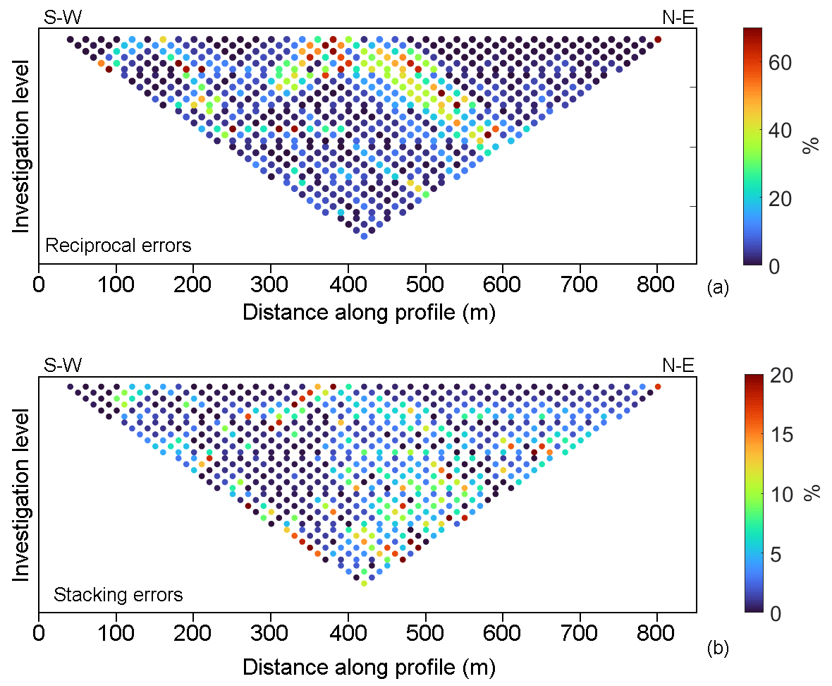
Figure 2 (a) Distribution of the percentage reciprocal errors. (b) Distribution of the percentage stacking errors calculated using DD direct measurements. The error magnitude is given by the colour scale placed on the right side of each panel. Note that the limits of the two colour scales are different.

A preliminary filter stage was performed by discarding measurements with an associated percentage reciprocal error larger than 40 %. Most of the discarded data were localized in the surficial part of the pseudosection, between 300 and 500 m along the profile. An additional filtering stage was based on the observation of resistivity data as a profile plot. Data characterized by abrupt resistivity variations and negative apparent resistivity values, probably due to the existence of large resistivity contrasts (Lee and Cho, 2020), were also filtered out. In total, almost 10 % of the original data were excluded during the filtering stages, with the filtered dataset characterized by a mean percentage reciprocal error of about 6 %.

A similar procedure was repeated on the starting (unfiltered) dataset, discarding measurements with an associated stacking error larger than 15 % and characterized by abrupt resistivity variations and negative apparent resistivity values. In total, almost 6 % of the original data were excluded during the filtering stages, with the filtered dataset characterized by a mean percentage reciprocal error of about 2.5 %.

The two adopted thresholds for the preliminary filtering stages (percentage reciprocal error larger than 40 % and stacking error larger than 15 %) have been chosen on a statistical basis in order to include all data whose errors were in the range [mean error (percentage or stacking) ± 2σ (standard deviations)].

Finally, topographical information was included in the dataset, which was inverted with the Res2DInv program (Geotomo Software; Loke and Barker, 1996). The resistivity models presented in what follows were obtained by using an L2 norm and directly inverting the apparent resistivity values that converged better.

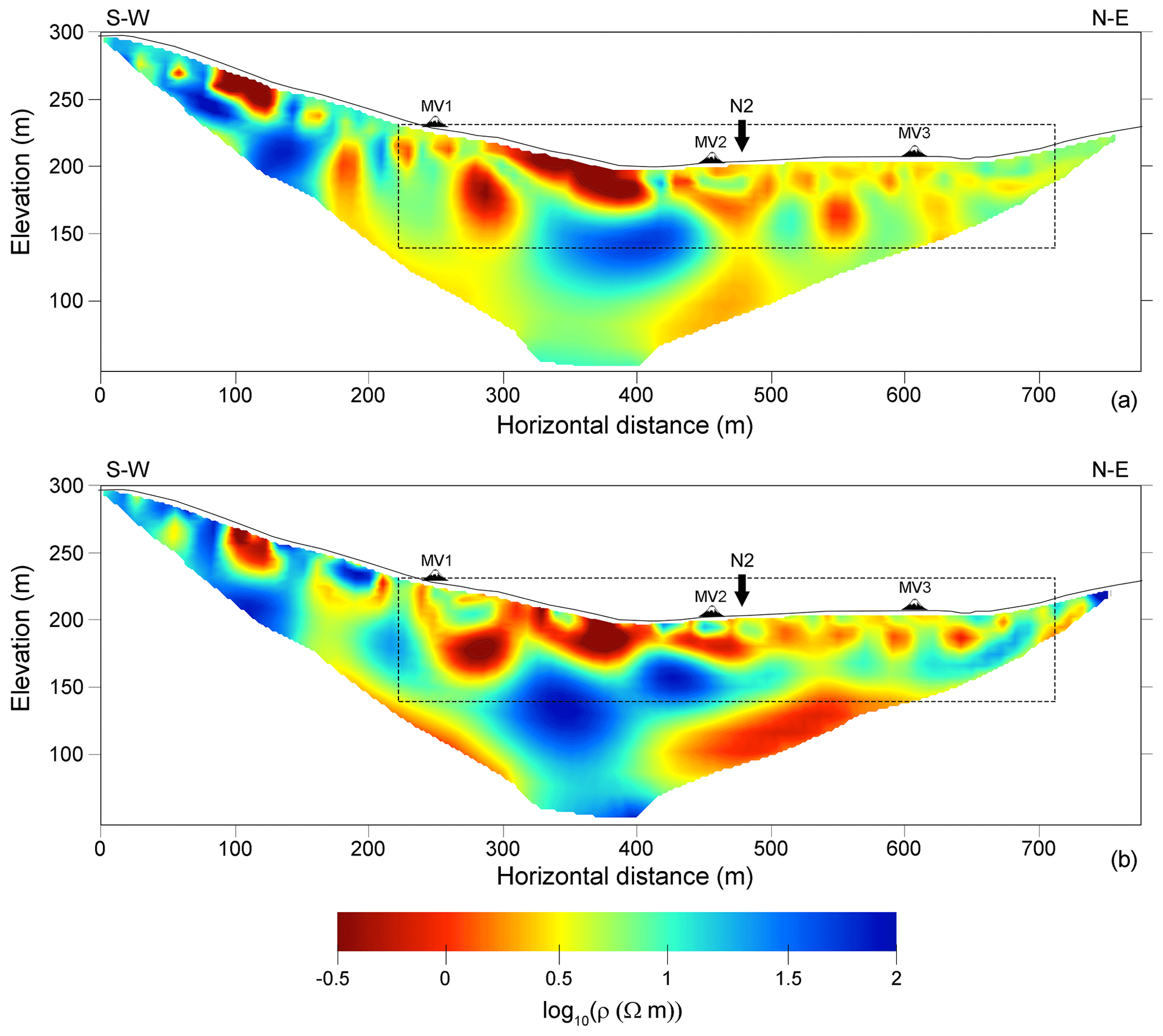
Figure 3 Resistivity models obtained integrating error estimates: (a) reciprocal errors and (b) stacking errors. The two models are presented with the same colour scale. In the panels, the locations of the mud volcanoes (MV1, MV2, and MV3), the crossing point between the ERT_N1 geoelectrical profile and the ERT_N2 ones (black arrow with the N2 label), and the subsoil portion investigated by Lupi et al. (2016) (identified by a dashed black line) are also reported.

The two models presented in Fig. 3 show the inversion results obtained, including in the inversion procedure both the reciprocal errors (Fig. 3a) and the stacking errors (Fig. 3b). The use of reciprocal errors in the inversion procedure leads to a model with a low rms value (4.8 %) and with resistivity contrasts smoother than those visible in the model with the stacking errors, which, being smaller than the reciprocal ones, also influenced the final rms errors (9.9 %). Generally, the models show a similar pattern of resistivity distribution within the subsoil where

• the SW part of the section is more resistive than the NE one;

• a highly conductive surficial anomaly placed between 300 and 400 m (horizontal distance) in the area is less constrained by the data due to filtering operations;

• there is a shallow highly conductive zone below the mud volcanoes, which is characterized by a lateral variability;

• there is an intermediate relatively resistive layer, which appears to be more continuous in the model obtained by integrating the stacking errors;

• two deep conductive zones are on the SW and NE bottoms of the sections.

Considering the similarity between the two models and assuming a higher reliability level for the one obtained by integrating the reciprocal errors, a comparison with the results of Lupi et al. (2016) is presented in Fig. 4. The colour scales adopted are similar although not the same; the differences, in any case, are not relevant for the sake of a visual comparison of the tomographic results. Furthermore, the elevation information in Lupi et al. (2016) with respect to ERT is not correct because it is shifted upwards by about 30 m. Generally, the two resistivity distributions can be considered consistent in the limits of their different spatial resolutions, of their investigation depths, and of the time span that occurred between the two datasets' acquisition (November 2012 for the dataset of Lupi et al., 2016; February 2022 for the dataset presented here). The presence of the “conductive domes” in the Lupi et al. (2016) section, marked D1–D3 in Fig. 4, is confirmed here as well as the existence of more resistive areas between them. The main differences are related to the conductive areas placed (a) in the shallow portion (20 m b.g.l.) of the resistivity image between mud volcanoes 1 and 2 (marked C1) and (b) in the elevation range 150–180 m a.s.l. between volcanoes 2 and 3 (marked C2). The first one (C1) may be an artefact of the inversion procedure and not a real feature of the subsoil. As already discussed in presenting Figs. 2 and 3, data involved in the inversion procedure that led to the conductive anomalies are those characterized by the largest experimental errors, both reciprocal and stacking. The same is not true for the second conductive anomaly (C2), which can be considered representative of a real condition of the subsoil that probably did not exist in 2012 when the surveys of Lupi et al. (2016) were performed.

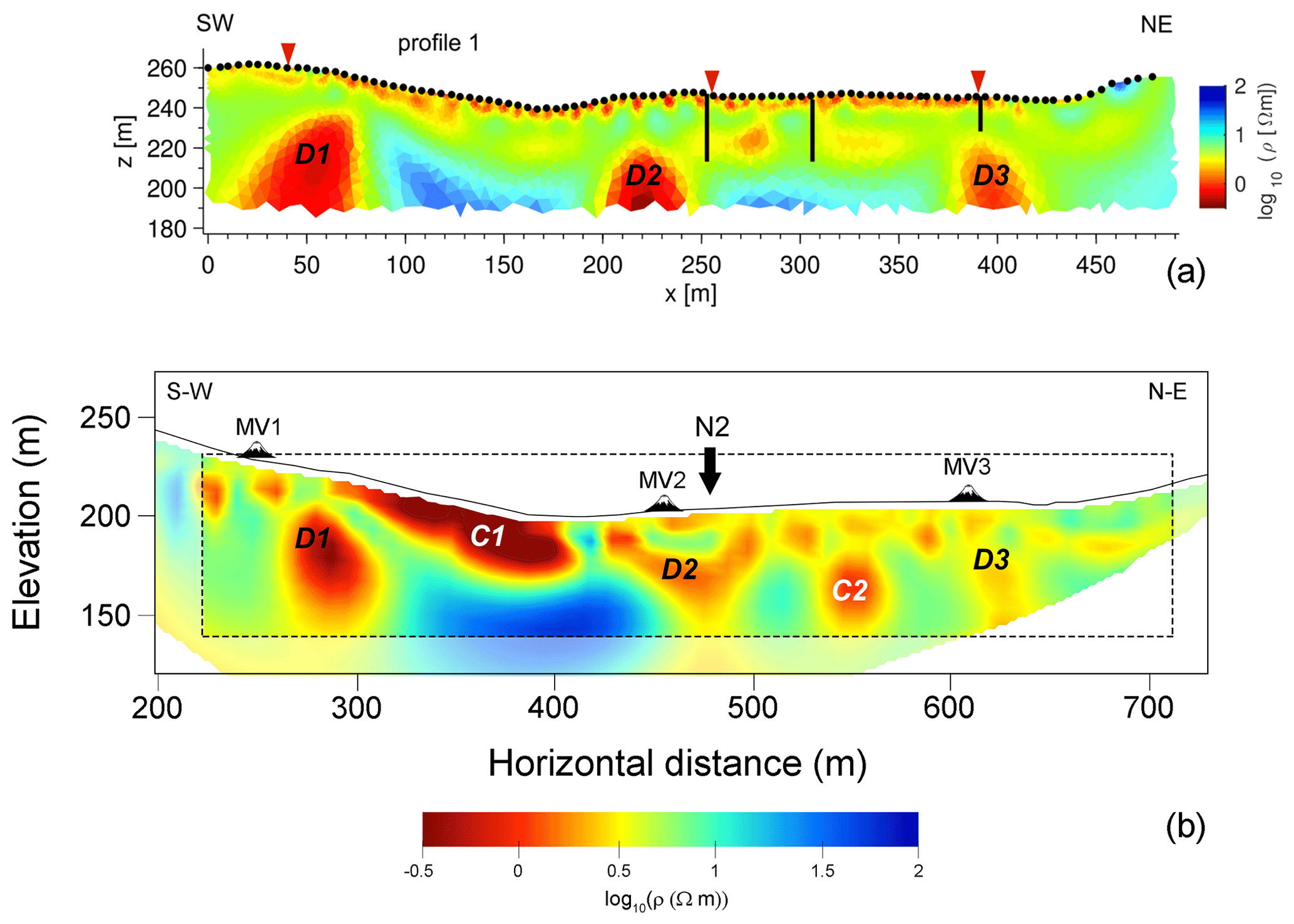
Figure 4 Comparison between Lupi et al. (2016) resistivity model (a) and the corresponding portion of the ERT_N1 DD resistivity model (dashed black line in b). The elevation information as well as mud volcano positions slightly differs in the two models. The meaning of the capital letters D1–D3 and C1–C2 is described in the text.

Wenner–Schlumberger and pole–dipole data inversion

As previously specified, for these datasets only stacking errors are available. The integration of the stacking errors into the inversion procedure, the lower noise level which usually characterizes these geoelectrical-array data, and the comparison with the DD inversion results are deemed to be sufficient to evaluate the reliability of the resistivity models.

As for DD data, the inversion procedure was preceded by the analysis of the contact resistances (Fig. 5a and c) and of the stacking-error spatial distributions (Fig. 5b and d). The WS dataset is characterized (Fig. 5a and c) by low contact resistances and low stacking-error values almost uniformly distributed along the profile and in depth (differently from what was observed for the DD dataset). The P-DD dataset had an electrode with a bad contact resistance (as highlighted by the two red bands in Fig. 5c and d). The P-DD data were acquired soon after the WS data, which show no evidence of bad resistivity contact. Thus, the observed worsening of the contact resistance is probably due to a tourist in the area who unplugged one of the electrodes. The stacking-error amplitude distribution agrees with the measuring conditions. Negative data were also removed from the plots in Fig. 5.

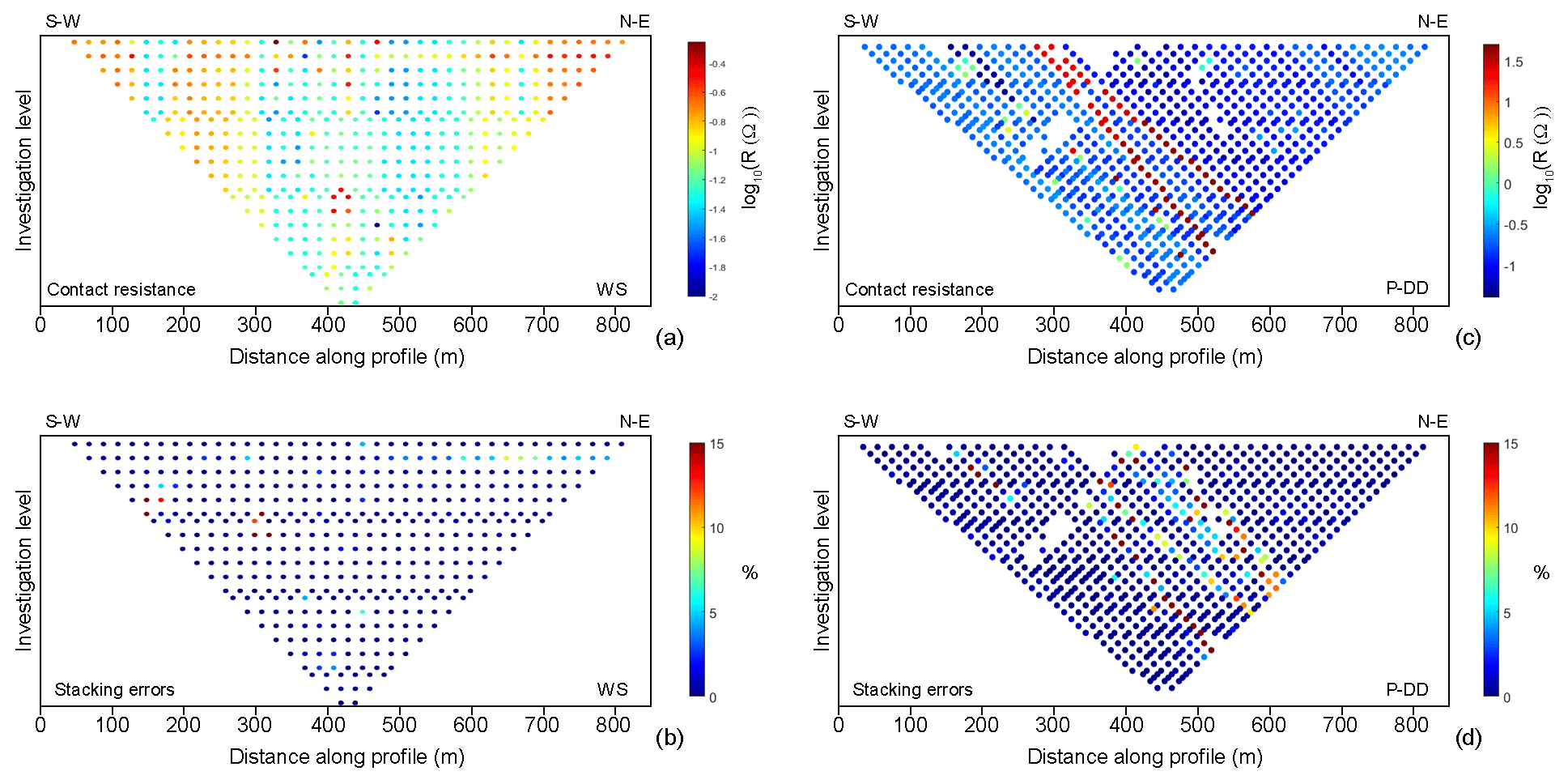
Figure 5 (a) Distribution of the contact resistances related to the WS dataset. (b) Stacking-error distribution of the WS dataset. (c) Distribution of the contact resistances related to the P-DD dataset. (d) Stacking-error distribution of the P-DD dataset. The contact resistances and error magnitude can be read on the colour scale placed on the right side of each panel. Note that, for the contact resistances, the limits of WS and P-DD colour scales are different. In the P-DD panels, the lack of dots in some areas of the distribution is due to the presence of negative resistivity data, which were filtered out from the dataset used for creating the figure.

The datasets were then filtered by eliminating data associated with a percentage stacking error higher than 5 %. This procedure removed less than 5 % of the data for the WS dataset and less than 7 % of the data for the P-DD dataset. The inversion results are shown in Fig. 6 along with the DD model previously shown in Fig. 3 (upper panel).

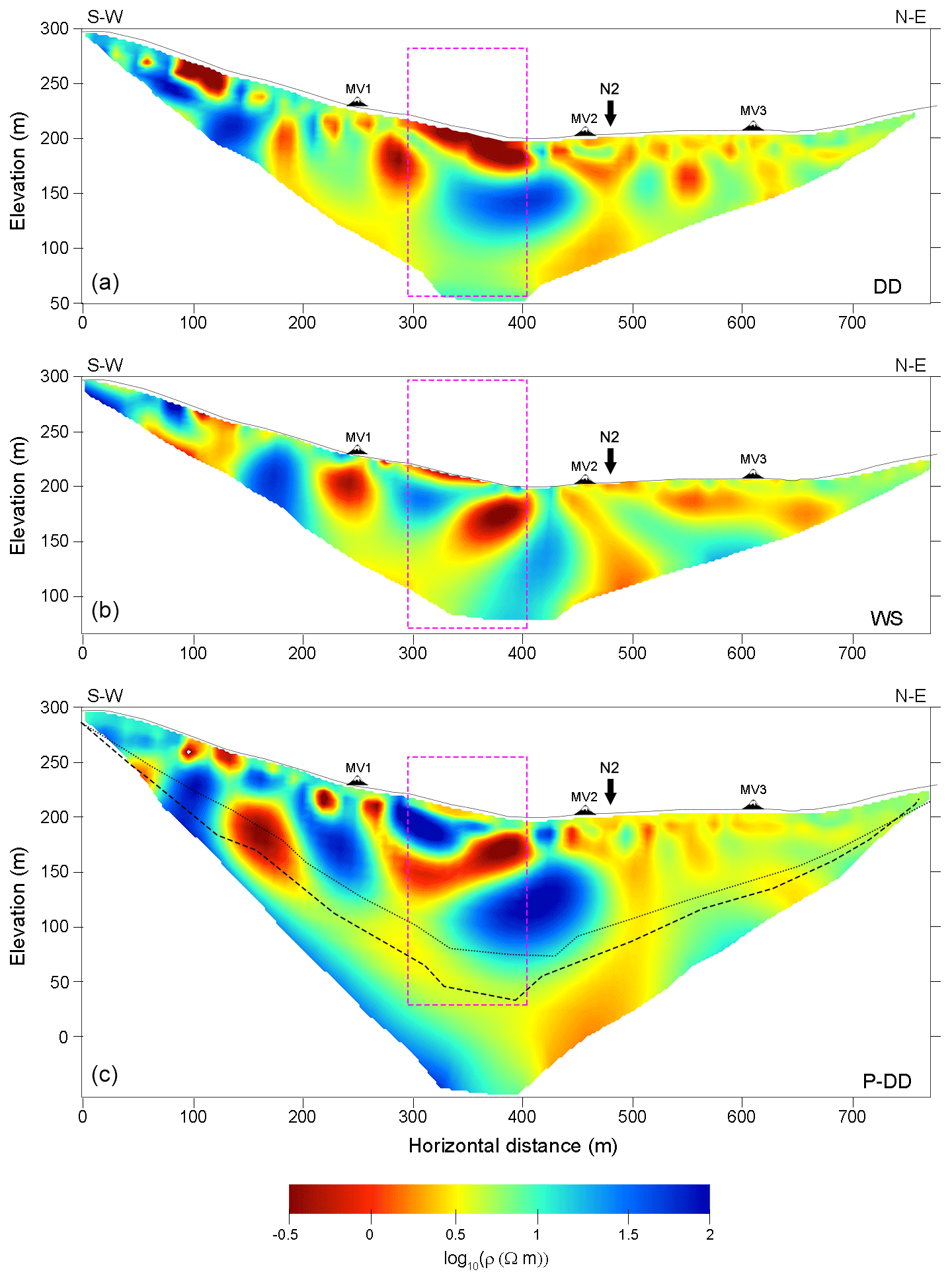
Figure 6 Profile ERT_N1: resistivity models obtained by inverting the DD dataset (a), the WS dataset (b), and the P-DD dataset (c). All models are presented using the same colour scale. The position of the mud volcanoes (MV1, MV2, and MV3) along the profile is marked on top of each section along with an indication (vertical black arrow) of the crossing point between the section ERT_N1 and the section ERT_N2. The dashed magenta rectangles indicate an area of higher dissimilitude between the tomographic results. The dotted and dashed lines shown in the P-DD section represent the subsurface area investigated by the WS and DD sections, respectively.

Considering the differences in terms of the sensitivity and vertical/horizontal resolution of the three adopted electrode configurations, the resistivity models (Fig. 6) show a general agreement in terms of both resistivity contrast and the spatial distribution of the electrical properties in the subsoil with an investigation depth, which, in the P-DD model, goes down to −50 m below sea level.

For distances along the profile <300 and >400 m, the P-DD and the DD models image a similar resistivity distribution within the subsoil. In these ranges, differences can be noticed between P-DD and DD models and the WS one, whilst between 300 and 400 m differences are found between PD and WS models and the DD one. We maintain that these differences can be ascribed to the following:

• The arrays have different sensitivity to lateral resistivity variation (much higher in the P-DD and DD models than in the WS model), and there is a substantial difference in data spatial coverage (DD and P-DD have a higher data coverage than WS; see Fig. 5). This, for example, may explain what was imaged in the datasets just below MV1 (Fig. 6). Here, the WS model depicts the presence of a unique conductive body, while P-DD and DD (with reciprocal errors) show the presence of two smaller conductive nuclei.

• The investigation depths are different. P-DD has an investigation depth which is almost double the one of WS. Thus, resistivity anomalies recovered at the bottom of the WS model are less reliable due to the lack of data in the deeper portion of the section. For example, the resistive nucleus depicted in the WS at about 180 m along the profile extends up to the lower limit of the sections. In the P-DD model, the same resistivity anomaly is confined at a shallower depth and overlays a conductive area (not imaged by WS due to the lack of deeper data).

• DD and P-DD differ in the area between 300 and 400 m (horizontal distance) (dashed magenta rectangle in Fig. 6). Here, the conductive surficial layer in the DD ERT is replaced both in P-DD and in WS by a less extended and less conductive area, whereas the deeper resistive area visible in DD is divided in two by a conductive anomaly (more continuous in the P-DD image). WS, as emerges from the analysis of the stacking-error distribution, is the only dataset which does not show any error value increase in this area. This condition ensures reliability of the resistivity distribution imaged in this area by the WS model and, by similarity, also by the P-DD model.

For these reasons, the geological and structural interpretation of the geoelectrical model will be performed on the P-DD one.

Before proceeding with the geological interpretation of the model, an additional test was performed to check if the use of an amplified stacking error, with an amplification factor of 2.4 (see the “Dipole–dipole data inversion” section), could produce relevant modifications of the inversion results. Keeping the filtering procedure unchanged and considering the stacking-error distribution (Fig. 5), the inverted WS dataset (with amplified errors) was composed of the same measuring points as those of the one used to obtain the model of Fig. 6 (central panel). Thus, no additional data were filtered out. The inversion produced a “new” WS resistivity model (not shown here) that has a lower rms compared to the model shown in Fig. 6 (central panel) but that is very similar to it with no relevant changes observable. As regards the P-DD datasets, by amplifying the stacking errors and keeping unchanged the filtering rules, a larger number of data were filtered out, especially in the central and shallow part of the section. The new resistivity model (not shown here) is hence almost the same as the one shown in Fig. 6 (lower panel) except for the shallow part between 300 and 400 m along the profile. In this area, the conductor is more pushed towards the surface. Also in this case, like for WS, the main features of the model do not vary significantly. We can hence conclude that, at least in this case, the stacking-error amplification does not modify the inversion results in a relevant way provided that the inverted dataset is unchanged. If the stacking-error amplification produces, as happened for the P-DD dataset, a dataset reduction (due to the adoption of filtering rules), modifications are observed. In this case, the more data that are discarded, the greater the inversion result difference will be.

3.2.2 ERT_N2 profile

For the ERT_N2 profile, the same approach as that used for the ERT_N1 profile was adopted, except for the comparison with previous and/or independent geophysical data. In Lupi et al. (2016), in fact, several profiles oriented as in ERT_N2 are presented, but they have a higher spatial resolution and lower investigation depth compared to ours, to be used as a reference point for a fruitful comparison. For the DD dataset, the mean percentage reciprocal error is 8.3 % and the mean percentage stacking error is 4.4 %. By integrating the two different error types into the inversion procedure, similar results, in terms of resistivity distributions, came out (not shown here). The reliability of the resistivity models is also ensured by the similarities between DD models and WS and P-DD ones (Fig. 7). All models show the presence of strong resistivity contrasts from 300 m (horizontal distance) till the end of the profile. In all models and in their central portion, a uniformly high-resistivity area is visible, which, as it emerges from the DD and from the P-DD sections, is confined in depths down to ∼100 m a.s.l. As discussed before for the ERT_N1 profile, DD and P-DD are more sensitive to horizontal resistivity variations and, hence, depict a more detailed resistivity distribution. For this reason, the geological and structural interpretation of the geoelectrical model will be performed on the P-DD one.

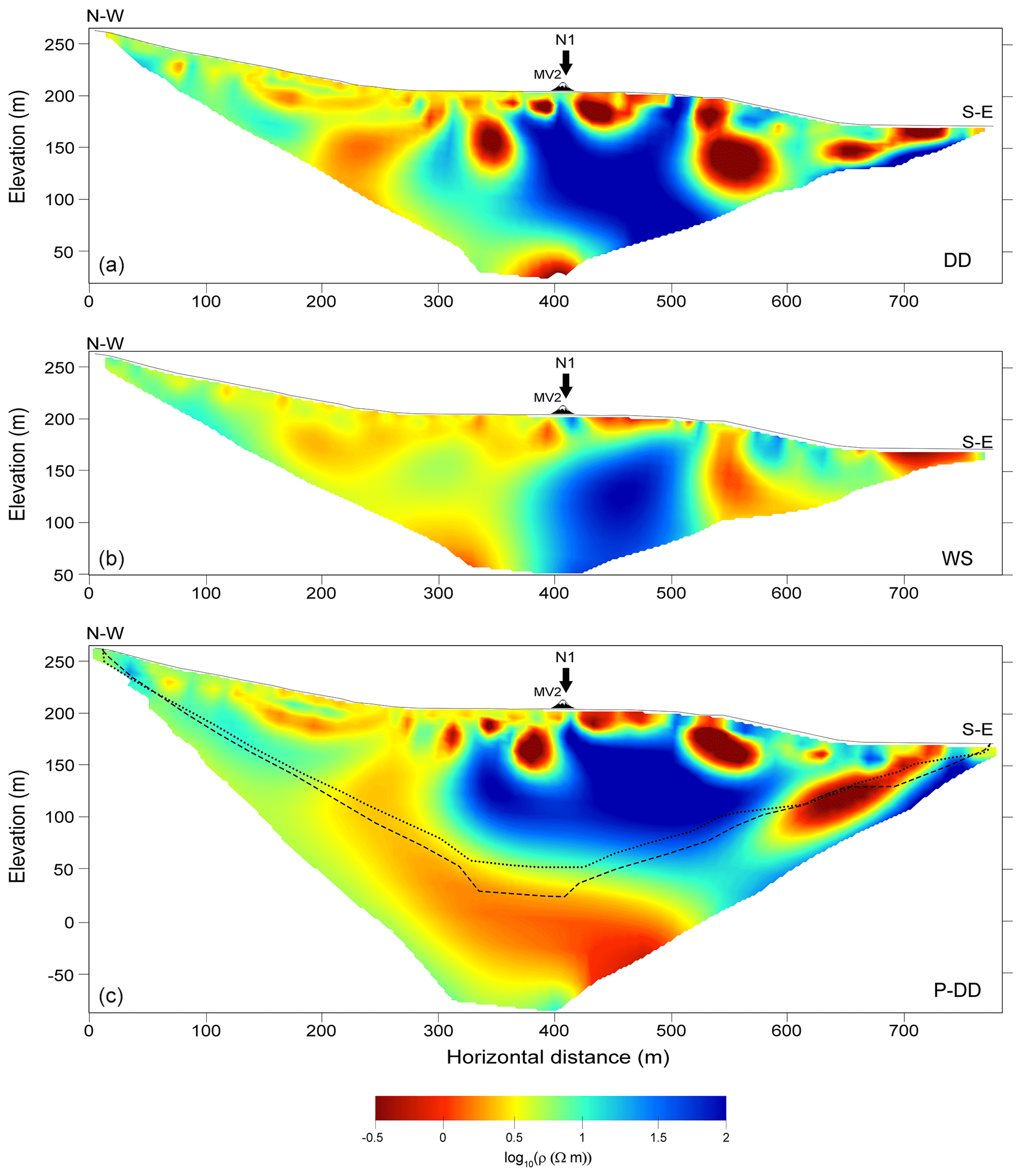
Figure 7 Profile ERT_N2: resistivity models obtained by inverting the DD dataset (a), the WS dataset (b), and the P-DD dataset (c). All models are presented using the same colour scale. The position of the mud volcano MV1, placed off profile at about 20 m from the ERT_N2 trace, is marked on top of each section along with an indication (vertical black arrow) of the crossing point between the section N2 and the section N1. The dotted and dashed lines shown in the P-DD section represent the subsurface area investigated by the WS and DD sections, respectively.

3.2.3 The 3D visualization of the ERT profiles

The spatial continuity of the two tomographic results and a clearer image of the resistivity distribution within the subsoil can be obtained by simultaneously plotting ERT_N1 and ERT_N2 (Fig. 8). This operation shows a good match between N1 and N2 with fairly good consistency between the two resistivity distributions in the common investigated portion of subsoil.

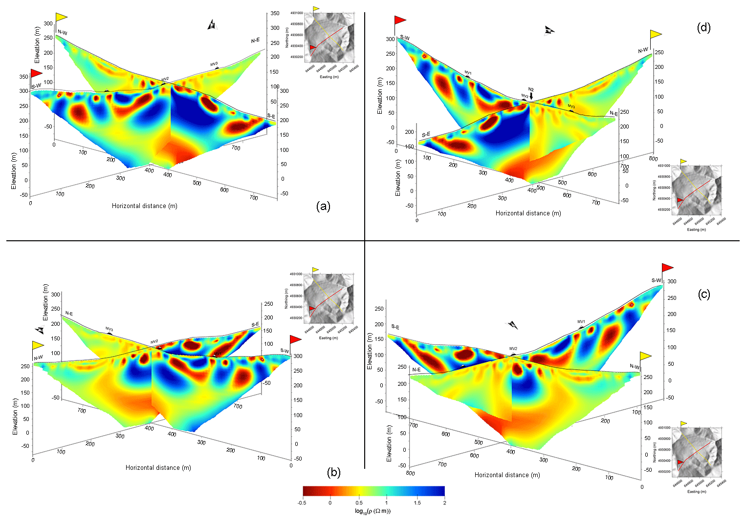
Figure 8 The 3D arrangements of the tomographic results. Starting from panel (a), an anticlockwise rotation of the tomographic result is performed. The yellow and red flags on top of each section indicate the starting point of the geoelectrical surveys. The inset in each panel shows the location of the survey.

Figure 8 also reveals how the northern sector of the Nirano Salse area strongly differs, in term of resistivity distribution, from the southern one. To the north, the subsoil is more homogeneous and generally conductive (ρ<10 Ω m). To the south, strong resistivity contrasts (both lateral and vertical) characterize the resistivity sections. Mud volcanoes are generally located over conductive anomalies.

4 Geological model

The interpretation of the two geoelectric pole–dipole profiles (Figs. 9 and 10) presented in this study allows us to shed some light on the structural setting of the Nirano area and propose a novel geological model that can account for the position of the vents, the vents' activity, and the morphology of the area.

Figure 9 Interpreted ERT_N1 profile. The capital letter “C” shows the location of the conductive anomalies associated with favourable routes for rising fluids. The capital letter “D” shows the location of the common conductive zone, possibly representing the Cigarello Fm clay unit. The capital letter “F” indicates the area probably associated with a fault zone.

Figure 10 Interpreted ERT_N2 profile. The capital letter “C” shows the location of the conductive anomalies associated with favourable routes for rising fluids.

The resistivity features recovered by the presented models will be discussed in terms of (i) geological boundaries, (ii) mechanical conditions (in terms of fracture presences), (iii) fluid presence, and (iv) fluid compositions.

The Miocene marly rocks and the Argille Azzurre (Pliocene FAA), the most relevant geological units expected in the area, are characterized by different electrical fingerprints, with the former generally more resistive than the latter. Fluid presence can affect the measured resistivity in a more complex way. In a first approximation, a gas phase is expected to enhance resistivity, whereas a liquid-phase electrical signature depends on the liquid type: saline fluids lower the resistivity, whereas hydrocarbons, for example, have the opposite effect.

4.1 SW–NE ERT_N1 section

The SW–NE ERT_N1 section is characterized by the presence of a shallow conductive layer (2–10 Ω m) that is associated with the Argille Azzurre outcrop (FAA). The SW portion of the model shows strong resistivity contrasts (ranging from 0.3 to 80 Ω m) down to about 50 m a.s.l. of elevation (from 0 to about 450 m of distance along the profile); the alternating resistivity anomalies often assume a subvertical elongated shape. In contrast, the NE portion of the model is mostly conductive (ranging from 2 to 20 Ω m) with a layered structure. It is worth noting that the passage between these two different resistivity distribution domains occurs in correspondence to the axis of a monocline or of a fault (horizontal distance about 500 m, grey-shaded rectangle in Fig. 9 labelled “F”) that may be related at depth to the structural trap for fluid accumulation (Bonini, 2007).

We interpret the subvertical resistivity contrast present towards the southwest as faults that spatially correspond well at faults also inferred by other authors (Bonini, 2008) (red arrows in Fig. 9). These faults slightly offset the base of the FAA represented by the dashed red line (Fig. 9).

The conductive layered structure towards the northeast is interpreted as the presence of multiple aquifers (low-resistivity areas, indicated in Fig. 9 by dashed blue lines) that agree well with the presence of sandy turbidite deposits in the FAA (Castaldini et al., 2017; Giambastiani et al., 2022) and are locally interconnected between vents MV2 and MV3.

A shallow subhorizontal connection also exists between vents MV1 and MV2 (labelled “C” in Fig. 9), albeit characterized by lower resistivity values. These very low resistivity values (as low as 0.3 Ω m) near MV1 and MV2 were also imaged by the shallow ERT model presented by Lupi et al. (2016) and were interpreted as reflecting the presence of high-salinity fluids. This interpretation, however, is not supported by recent fluid conductivity measurements performed directly in situ at some vents (Giambastiani et al., 2022; Oppo, 2011; Oppo et al., 2013) with conductivity values ranging between 10 and 21 mS cm⁻¹ (which corresponds to a resistivity value ranging from 0.5 to 1 Ω m), typical of brackish water.

To justify the observed low resistivity values at depth, it is thus required to add at least another conductivity phase (Glover and Hole, 2000). We explore two possibilities. The first one is the clay content and surface conductivity phase. In saturated soil, the electrical current flows by means of ions that are present in the saturating fluid (brine). If the grain size is very small, such as in clay, the electrical current will easily flow through the pore fluid, making it less resistive. Particle size distributions of mud samples collected in some of the gryphons (Giambastiani et al., 2022) support this extra conductive phase as they indicate the presence of about 35 % clay and 56 % silt and the remainder sand. The second possibility for consideration is the presence of iron sulfides (pyrite) due to precipitation of hydrogen sulfide (H₂S). Supporting this condition is the low amount of H₂S at the surface among both the emitted gas and solutions, since it can precipitate as iron sulfides due to the largely available iron in the siliciclastic sedimentary units (Oppo, 2011; Oppo et al., 2013). Thus, we can interpret the very low resistivity anomaly C as a very shallow reservoir hosting brackish water and a place where one of the above-mentioned conductivity phases is acting.

The subvertical low (NE) (“F” in Fig. 9) and very low (SW) (“C” in Fig. 9) resistivity anomalies, here interpreted as favourable routes for rising fluids, converge deeply (above 50 m elevation) towards a common deep conductor (“D” in Fig. 9). This common conductive zone may represent the Cigarello Fm clay unit (Gasperi et al., 2005).

4.2 NW–SE ERT_N2

The NW–SE ERT_N2 section (Fig. 10) is almost parallel to the axis of the anticline. In this section, we also observe a relevant heterogeneity in resistivity distribution. Like in NE–SW ERT_N1, the NW portion of the section is regular and shows the presence of a subhorizontal stratification, which may indicate the presence of several aquifers (dashed blue lines in Fig. 10). The SE portion of the model shows more enhanced resistivity contrasts than the SW portion of the ERT_N1 model but with a less complex pattern. The transition between the more regular NW portion and the more heterogeneous SE is spatially coincident with the presence of the fault zone (two central red arrows in Fig. 10) also described in ERT_N1, which forms a small angle with this section. Indeed, down to 50 m elevation, local shallow conductive zones are hosted in a resistive layer that is sharply interrupted in the southeasternmost area, at about 650 m along the profile, where we infer the presence of a fault (blue arrow) whose surface intersection is located near a dry gas seep (yellow arrow in Fig. 10). This fault may be related to NE–SW-trending faults that are strike-slip transfer structures reported by Gasperi et al. (2005) in this area (blue arrow in Fig. 10). Thus, we interpret the resistive layer as the Termina marls and Pantano Fm (Miocene) unit that hosts local conductive anomalies associable with very shallow fluid reservoirs. In the deeper part of the model, along the whole profile, a deep conductor gently dipping towards SE is imaged. This conductive zone spatially coincides well with the one recovered in ERT_N1 and thus is interpreted as Cigarello Fm claystone (Gasperi et al., 2005).

Summing up, the resistivity features recovered by the two models matched well in the intersection area. Interestingly, an undisturbed layered system characterizes the northern sector (NW and NE) of the Nirano area in contrast to a more heterogeneous (SE) and even chaotic (SW) resistivity distribution in the southern sector. These major heterogeneities are located just where the “bowl” morphology is also irregular: in the SE corner a small creek cuts across the rim, and two relatively NW–SE-oriented steep ridges border the southwestern flank of the circular structure. It could be speculated that regional NW–SE- and NE–SW-oriented faults interacting and interfering with each other contribute to the formation of the geomorphological bowl. The tomographic images, in fact, suggest the presence of linear faults and fracture zones and not of circular structures as previously speculated by Bonini (2012) and Sciarra et al. (2019). These are important observations, because they do not support a gravitational collapse of the bowl area as previously assumed. On the other hand, the deepest parts of both models (below 70 m elevation) share a common conductive feature, associated with a clayey horizon (Cigarello Fm) that may act as an impermeable horizon for deep rising fluids. These deep fluids can reach the surface only where the fault zone breaks this sealing unit, allowing for gas and mud venting at the surface.

5 Conclusions

The geophysical investigation performed in the Nirano Salse provided new information on its deep structure. The pole–dipole geoelectric sections showed the existence of different structural conditions in the bowl-shaped morphology of the area. The northern sector of the Nirano subsurface seems to be characterized by a regular vertical stratification which can be associated with the presence of multilayer aquifers within the Argille Azzurre Fm. The southern sector, on the contrary, is dominated by the presence of subvertical discontinuities which can be associated with faults and fracture zones. In the geoelectrical sections, conductive zones can be associated with fluid accumulation areas. Fluid presence, however, is not sufficient to justify the extremely low resistivity values observed in both sections. We suggest that the low resistivity values may be associated with (i) clay content and the surface conductivity phase and/or (ii) the presence of iron sulfides (pyrite) due to precipitation of hydrogen sulfide.

Regardless of what the explanation for the observed resistivity values is, the areas containing fluids (gas and water) are in the shallow portion (50–100 m) of the subsoil and correspond to the main mud volcanoes. It is therefore reasonable to assume that these fluid accumulation zones constitute the surficial reservoirs of volcanoes. A larger-scale geophysical survey could disclose the existence of deeper fluid storage and its relationship with these shallow and localized reservoirs. The shallow fluid reservoirs have a relatively small volume and they are sparse in the sections, clearly showing that there is not a shallow fluid caldera below the Nirano Salse. This observation has important implications for the safety of the site. The most hazardous areas, in fact, are those closer to the mud vents where the shallow small reservoirs are located and not the whole area of the bowl. This could help pinpoint routes for tourists' access and fence out areas of potential liquefaction and mud eruption. This methodology for assessing local hazard could be extended to other mud volcano areas around the world.

The geoelectrical sections also highlighted the presence of faults, which are linear features oriented like most of the structures in this sector of the Apennines (NW–SE) and are not circular-collapse rim faults as previously thought. Likely, they provide gas/fluid flow routes from deep sources to the shallow reservoirs and finally to the mud volcanoes. A relevant example can be the major fault zone in the central portion of ERT_N1, which could be thought of as the main pathway along which fluids and gas reach the surface from their deep reservoirs (located beyond the ERT investigation depth limit). This major fault zone also offsets the Argille Azzurre Fm (FAA) down to the NE, and it accommodates deformation along the monocline flexure, which is well exposed north of the Nirano Salse.