Large-scale risk assessment on snow avalanche hazard in alpine regions

Snow avalanches are recurring natural hazards that affect the population and infrastructure in mountainous regions, such as in the recent avalanche winters of 2018 and 2019, when considerable damage was caused by avalanches throughout the Alps. Hazard decision makers need detailed information on the spatial distribution of avalanche hazards and risks to prioritize and apply appropriate adaptation strategies and mitigation measures and thus minimize impacts. Here, we present a novel risk assessment approach for assessing the spatial distribution of avalanche risk by combining large-scale hazard mapping with a state-of-the-art risk assessment tool, where risk is understood as the product of hazard, exposure and vulnerability. Hazard disposition is modeled using the large-scale hazard indication mapping method RAMMS::LSHIM (Rapid Mass Movement Simulation::Large-Scale Hazard Indication Mapping), and risks are assessed using the probabilistic Python-based risk assessment platform CLIMADA, developed at ETH Zürich. Avalanche hazard mapping for scenarios with a 30-, 100- and 300-year return period is based on a high-resolution terrain model, 3 d snow depth increase, automatically determined potential release areas and protection forest data. Avalanche hazard for 40 000 individual snow avalanches is expressed as avalanche intensity, measured as pressure. Exposure is represented by a detailed building layer indicating the spatial distribution of monetary assets. The vulnerability of buildings is defined by damage functions based on the software EconoMe, which is in operational use in Switzerland. The outputs of the hazard, exposure and vulnerability analyses are combined to quantify the risk in spatially explicit risk maps. The risk considers the probability and intensity of snow avalanche occurrence, as well as the concentration of vulnerable, exposed buildings. Uncertainty and sensitivity analyses were performed to capture inherent variability in the input parameters. This new risk assessment approach allows us to quantify avalanche risk over large areas and results in maps displaying the spatial distribution of risk at specific locations. Large-scale risk maps can assist decision makers in identifying areas where avalanche hazard mitigation and/or adaption is needed.

1 Introduction

In densely populated mountainous landscapes with continuous socio-economic growth and changing climate conditions, society is increasingly exposed to natural hazards (Zgheib et al., 2020). In mountainous regions such as the Alps, avalanches are a significant natural hazard in winter, causing damage to buildings and infrastructure. In the past 20 years, Alpine countries such as Switzerland have experienced multiple catastrophic avalanche situations. The winter of 2017/18 was the first since the catastrophic avalanche winter in 1999 (Wiesinger and Adams, 2007), during which the highest avalanche danger, level 5, was forecasted for wide areas across the Swiss Alps. In January 2018, 2.5 to 5 m of snow fell at higher altitudes within 25 d. Numerous avalanches in the categories “large” and “very large” were counted (Zweifel et al., 2019). In total, over 380 avalanches damaged buildings, traffic routes, or important infrastructure in Switzerland (Bründl et al., 2019), making it the most severe avalanche winter in recent years. This was also the case in Austria and Germany (MeteoSchweiz, 2019; Pancevski, 2019; ZAMG, 2020; Trachsel et al., 2020). In the following winter of 2018/19, exceptional snowfalls again occurred, causing substantial damages throughout Switzerland (Trachsel et al., 2020). Such events show that even in highly developed, well-adapted countries, society is still vulnerable to avalanches. Strategies, methods and risk assessments to counteract this threat are well developed in most areas in the Alps, but they need to be continuously developed to strengthen and improve the resilience of the population and its assets (Zgheib et al., 2020).

To cope with natural hazards threatening exposed assets, various organizations have introduced the concept of risk to the field of natural hazards. The IPCC (Intergovernmental Panel on Climate Change) for instance defines risk as the likelihood of the disturbance of the normal functionality of a society due to a hazardous physical event under vulnerable social conditions (vulnerability) with economic, material, or environmental consequences (IPCC, 2014), see also Fig. 1. According to this definition, the risk concept can also be applied to events with harmful consequences to the environment and environmental systems. Considering the impacts of natural hazards on the environment is also important to us. However, since damage to human life and man-made objects is of greater direct importance to society and decision makers, this concept is generally applied to infrastructure and buildings, as it is in this study.

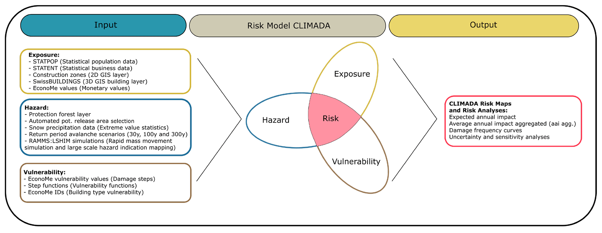
Figure 1 A schematic illustration of the applied IPCC risk concept, with the used input components for generating the base information on exposure, hazard and vulnerability, used to create risk maps and perform risk analyses.

The concept of risk was introduced in Switzerland in the late 1990s to support decision makers with dealing with natural hazards (Heinimann et al., 1998; Borter, 1999; Bründl et al., 2009). The risk concept also became the central element of the strategy for natural hazards of the National Platform Natural Hazards (PLANAT) in Switzerland (PLANAT, 2009, 2018). Overviews of natural hazard risks and vulnerabilities at different spatial scales were generated by various organizations in the last decade (MATRIX Consortium, 2013; van Westen and Greiving, 2017; Fuchs et al., 2019; FOEN, 2020). These studies vary from vulnerability surveys (Fuchs et al., 2015) to multi-risk and resilience approaches (Kappes et al., 2012; Komendantova et al., 2016). Projects such as RoadRisk, carried out by the Swiss Federal Roads Office, or the National Risk Overview, initiated by the Swiss Federal Office for the Environment (FOEN, 2020), were created laboriously. Such projects underline the need for large-scale risk surveys.

A method to assess avalanche risk at a regional or national scale is currently lacking, with a state-of-the-art hazard mapping tool to allow decision makers to identify hotspots of avalanche risk. The risk maps produced by this approach would show detailed short-term assessments to facilitate risk management decisions.

The goal of this study is to present a framework for assessing avalanche risk over widespread areas, as shown in Fig. 1. The method was applied in a regional case study in central Switzerland but can be deployed anywhere worldwide. Such a framework can also be useful to identify and visualize changes of the components of risk, such as hazard, exposure and vulnerability, over time and space. In this paper, we focus on the presentation of the framework for the current risk situation, which will serve as a baseline for modeling expected climate and socio-economic-induced changes of risk in future.

New strategies and tools to systematically identify risk and respond to threats in exposed areas are of increasing importance, especially in the context of climate change and population growth (IPCC, 2012). Changes in the climate system and their influence on local weather phenomena do not only affect us now (CH2018, 2018) but also will likely lead to an increase of the frequency and magnitude of natural hazards in the years to come (IPCC, 2014). In particular, various studies indicate that changes in the climate system, such as rising temperatures and an increase of extreme precipitation events, will likely influence gravity-driven hazards (Mani and Caduff, 2012; Ballesteros-Cánovas et al., 2018), including snow avalanches.

2 Methods

2.1 Risk

In the context of natural hazards in Switzerland, risk is defined as the product of hazard potential, objects at risk (exposure) and their vulnerability (Borter and Bart, 1999). In more detail, Bründl et al. (2016) define risk as the damage that is statistically expected due to the hazard intensity (caused by avalanche impact pressure) in a given scenario, calculated as the product of the expected damage and the frequency (1$/$return period) of this scenario.

In this study, the risk tool CLIMADA is used for risk assessment, and therefore we use the definition of the framework developers. It is a similar but extended definition of the IPCC risk concept by Aznar-Siguan and Bresch (2019), expressing risk as the probability of a consequence resulting from a hazard and its severity:

$$\begin{array}{}\text{(1)}& \text{risk}=\text{probability}\times \text{severity},\end{array}$$

where

$$\begin{array}{}\text{(2)}& \begin{array}{rl}\text{severity}=& F\left(\text{hazard intensity, exposure, vulnerability}\right)\\ =& \text{exposure}\\ & \times \text{vulnerability function}\left(\text{hazard intensity}\right).\end{array}\end{array}$$

The methods chapter is organized into subsections explaining all components of the risk framework from hazard, exposure and vulnerability to risk, and its application to the case study region (Sect. 2.2) in detail. These subsections contain the information on how the respective components were defined and generated in this study and how they are used to calculate the spatially distributed monetary terms of risk. Before going into detail, we will give a brief overview of those components. The hazard (Sect. 2.3) is obtained by avalanche hazard mapping using the RAMMS::LSHIM (Rapid Mass Movement Simulation::Large-Scale Hazard Indication Mapping) method. For this purpose, a protection forest layer (Sect. 2.3.2) is generated that defines where a protection forest is located. Using this layer, potential release areas can be identified with an automatic algorithm (Bühler et al., 2018b). Using extreme value statistics, maximum 3 d snowfalls are analyzed, and three avalanche scenarios with return periods (rp's) of 30, 100 and 300 years are defined (Sect. 2.3.1) and integrated into the release area calculation and also protection forest creation. With the defined potential release areas and an assigned amount of snow, the RAMMS (Sect. 2.3.4) avalanche simulations can now be carried out and a hazard indication map, showing avalanche impact pressures, can be generated.

The exposure (Sect. 2.4) is a dataset that defines the exposed monetary values. It consists of statistical data on the resident population and economic data. These are available in a GIS dataset with coordinates. Furthermore, Swiss building zones and a 3D building dataset are used. Monetary values are then assigned using the Swiss standard risk methodology “EconoMe” (FOEN, 2021) (Sect. 2.4.1). The third component is the vulnerability (Sect. 2.5), which defines assets' sensitivity to damage from avalanches with certain impact pressures by using a so-called impact or vulnerability function (Sect. 2.5.1). To express these components in numbers in the context of the risk concept (Sect. 2.1), the CLIMADA (Sect. 2.1.2) (climate adaptation) risk model is used. This model allows us to express the risk in monetary terms, such as the expected annual impact as well as the aggregated average annual impact, and depict them on spatial risk maps (Sect. 3.1). These values can also be presented in damage-frequency curves (Sect. 3.3) to show the return period at which monetary losses would be expected. A sensitivity and uncertainty analysis (Sect. 2.6.1) completes the risk assessment and shows the limitations of the framework.

2.1.1 Damage-frequency curves

Similar to exceedance-frequency curves which are a standard method in natural hazard risk analysis for plotting losses against a specific exceedance-frequency for historic events (Vogel et al., 2007), the damage-frequency curve plots the calculated damage against the return period. We use these curves to show synthetically generated avalanche risk scenarios and to draw conclusions between calculated damages. Therefore, we show possible outcomes at other return periods that have not been specifically calculated but rather estimated through interpolation. These curves thus provide a more complete picture and give decision makers a wider range of available interpretations of the results.

2.1.2 CLIMADA

CLIMADA is an open-source and open-access Python package for probabilistic risk assessment (Aznar-Siguan and Bresch, 2019). It allows the impact computation of natural hazards using intensity maps, considering exposure and its vulnerability. It is possible to compute current and future risk, including climate change, that modifies the hazard and socio-economic development affecting the exposures and vulnerability. Finally, one can compute the reduction in risk and cost from adaptation options to perform a cost-benefit analysis (Kropf et al., 2021). For all the model outputs, CLIMADA provides a module to perform uncertainty and sensitivity analyses (Kropf et al., 2022) using global (quasi-)Monte Carlo sampling.

In this project, we use CLIMADA to compute the risk of avalanches to more than 13 000 individual buildings from each of the 40 000 simulated avalanches using the hazard intensity maps described in Sect. 2.3, the exposures distribution described in Sect. 2.4 and the impact functions introduced in Sect. 2.5. As defined in the CLIMADA tool (Aznar-Siguan and Bresch, 2019), the impact is expressed by the following risk quantities.

• The expected annual impact for each exposure (affected building) is expressed in monetary terms per year (Swiss Francs (CHF) per year). It combines the hazard intensity with its expectation (return period) and the damage degree from the impact functions.

• The average annual impact is the average of the expected annual impacts overall exposures, expressed in monetary terms per year (CHF per year).

• The average annual impact aggregated is the sum of the average annual impacts for each scenario or all scenarios combined, expressed in monetary terms per year (CHF per year). The average annual impact aggregated corresponds to the overall risk.

2.2 Case study region

For this study we focus on an area in the Gotthard region (Fig. 2) in central Switzerland between Altdorf and Göschenen (Canton of Uri), one of the most important north–south transit corridors in Europe. The Gotthard area is one of the snowiest regions in Switzerland and is characterized by many steep, unforested slopes of different orientations with high avalanche activity. Steep meadows or rocky slopes form avalanche release areas with 28 to 50^∘ slopes in the upper catchment area of the main Reuss Valley and range from an elevation of approx. 1700 m a.s.l. up to almost 3000 m a.s.l. During heavy snowfall, avalanches start in the backcountry release zones and sometimes flow down to valley bottom, where the snow masses are deposited in the Reuss river bed. To perform avalanche risk analyses we use snow depth increase data from the SLF station Meien ME2 (see Fig. 2). This station has a 66-year record and includes extreme snowfalls (e.g., winters 1950/51 and 1998/99), making the data basis more reliable for extreme events. It is located in the center of the study area at an elevation of 1320 m a.s.l. and thus provides a good data basis for avalanche assessment.

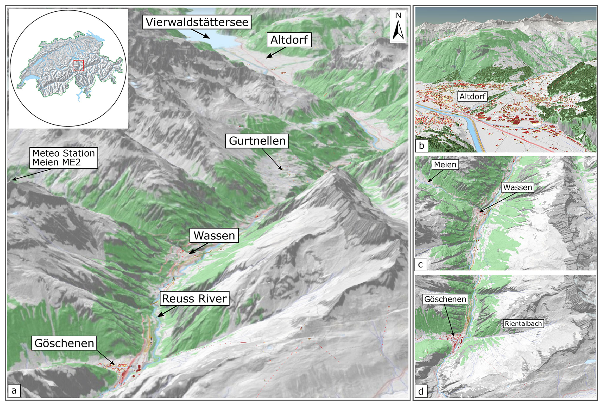
Figure 2 Illustration of the case study area of the Gotthard region in central Switzerland with avalanche-prone slopes. (a) Overview of the region, with a map panel of Switzerland. (b) Detail of the village Göschenen, with the well-known Rientalbach avalanche path. (c) Hazard hotspot Wassen. (d) Altdorf and its surrounding slopes. Forests are shown in green and buildings in red. Map base data source: Swiss Federal Office of Topography (https://map.geo.admin.ch, last access: 5 February 2023).

2.3 Hazard – avalanche hazard indication mapping with RAMMS::LSHIM

Hazard indication mapping of snow avalanches at scales of 1:5000 to 1:10 000 has been carried out for backcountry users (Harvey et al., 2018) and exposed communities in Switzerland (Bühler et al., 2022), Italy (Maggioni et al., 2018; Monti et al., 2018) and other regions worldwide (Bühler et al., 2018b). To cover all possible avalanches affecting the region, every hydrological catchment stretching from the main valley up to the mountain ridges of the side valleys was included in our assessment. The individual catchments were combined into a large comprehensive perimeter outlining the study area (Fig. 4). To identify relevant catchment areas that are particularly affected by avalanches, a dataset of all past reported avalanches leading to damage, observed and recorded by the WSL Institute for Snow and Avalanche Research SLF and cantonal and federal authorities, were used. The selection of the hydrological catchment areas also includes areas without avalanche records but which were regarded as relevant for hazard indication mapping in this study.

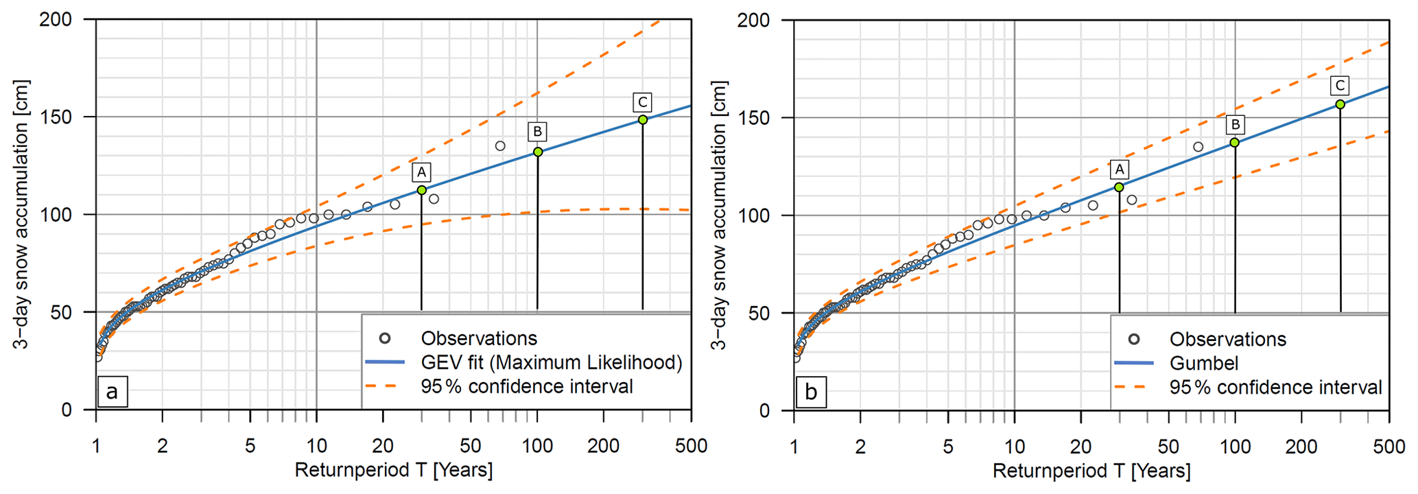
Figure 3 Extreme value statistics of the 3 d snow depth increase data (ΔHS3) of the meteo-station Meien (1320 m a.s.l.) for determining scenario return periods. (a) Generalized extreme value distribution with maximum likelihood estimations (GEV-MLE) for return period scenarios: [A] is 30, [B] is 100 and [C] is 300 year. (b) Gumbel (GUM-MLE) distribution with maximum likelihood estimations for return period scenarios: [A] is 30, [B] is 100 and [C] is 300 year, see Table 1.

2.3.1 Definition of three avalanche scenarios

To cover a large range of potential avalanche events, we consider three different avalanche scenarios (see Table 1). One frequent scenario [A] corresponding to a snowfall event with a 30-year return period, one intermediate one [B] (100-year return period) and one extreme [C] scenario (300-year return period). The definition of the scenarios is implemented according to the maximum 3 d snow depth increase and directly determines the mean fracture depths and thus the release volume and the modeled avalanche run-out lengths. The higher the return period, the larger the mean avalanche volume. The term return period (rp) describes the average number of years between two comparable events of the same intensity at the same location. By hazard frequency we denote the probability of occurrence calculated as a reciprocal value of the return period (1$/$rp). This definition is common practice in avalanche hazard mapping (PLANAT, 2009; Salm et al., 1990). To look at the overall avalanche risk of all scenarios later in the risk analysis, we adjusted the three avalanche scenarios for the combination with regard to the return period by $p_{\mathrm{30}}=p_{\mathrm{30}}-p_{\mathrm{100}}=\mathrm{1}/\mathrm{30}-\mathrm{1}/\mathrm{100}=\mathrm{0.0233}$ and $p_{\mathrm{100}}=p_{\mathrm{100}}-p_{\mathrm{300}}=\mathrm{1}/\mathrm{100}-\mathrm{1}/\mathrm{300}=\mathrm{0.00667}$ and $p_{\mathrm{300}}=\mathrm{1}/\mathrm{300}=\mathrm{0.0033}$. This allows us to combine the hazard scenarios and recalculate the overall risk, such as the expected annual impact for single objects over all hazard scenarios in the entire study region.

Table 1 Δ 3 d snow depth accumulation (cm) at the weather station Meien (1320 m a.s.l.) in Canton of Uri.

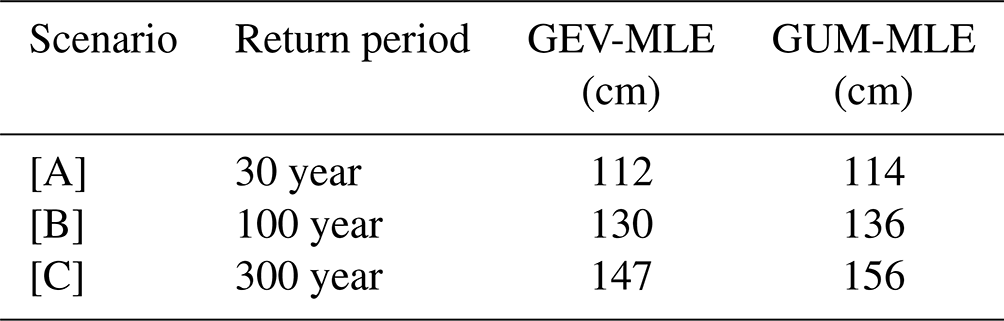
The derivation of the 3 d snow depth increase was based on a long-term snow measurement series at the meteorological station named “ME2”, representative of the chosen area. As shown in Fig. 3, two extreme value statistical methods were applied: the generalized extreme value distribution with maximum likelihood estimations (GEV-MLEs) and the Gumbel distribution (Bocchiola et al., 2008) with maximum likelihood estimations (GUM-MLEs). Table 1 shows that both methods produce similar values, but slightly higher values are produced with Gumbel. This depends on the choice of the fitted correlation through the value distribution. Since the Gumbel distribution rather represents a “worst case” for the respective return period, and Bocchiola et al. (2008) confirms the application of this method, these values were chosen for avalanche fracture depth determination. To account for elevation of the release area, a correction factor has to be applied. Blanchet et al. (2009) estimated this factor to be about ±2 cm per 100 elevation meters, whereas Swiss practitioners usually use a gradient of 5 cm per 100 elevation meters (Margreth et al., 2008). In consideration of the large avalanche scenarios, we applied 5 cm per 100 elevation meters to each release polygon, corresponding to existing studies in the Swiss Alps (Bühler et al., 2022). This elevation correction was applied based on the reference elevation of the measuring station ME2 at 1320 m a.s.l. This correction was calculated for each individual release area based on the difference between the respective mean elevation of an avalanche release area and the elevation of the measuring station ME2. Since the 3 d snow depth increase (see Fig. 3) at the meteorological station Meien is measured in flat terrain, a standard slope inclination correction (Salm et al., 1990; Margreth, 2007) was conducted for all avalanche release polygons to consider an adapted fracture depth d0. As is standard in avalanche practice, we assume that less snow accumulates in steep terrain than in flat areas. Depending on the average inclination of the individual release area, the slope correction factor of the snow height for each potential release area is individually calculated and corrected. This is applied automatically in the ArcGIS Python script for fracture depth d0 calculation by using a slope factor ψ generally depending on the snow strength (increasing with snow depth) $\mathit{\psi }=\mathrm{0.291}/\sin \left(\mathit{\alpha }\right)-\mathrm{0.202}\times \cos \left(\mathit{\alpha }\right)$, with α being the slope angle (Salm et al., 1990; Gruber and Margreth, 2001; Bühler et al., 2018b) and the fracture depth d0 being a function of the 3 d snow depth increase d0^* and the slope factor ψ, expressed as $d\mathrm{0}=d{\mathrm{0}}^{*}f\left(\mathit{\psi }\right)$ (Salm et al., 1990). To correct for the influence of blowing snow, a snow drift factor was added, depending on the scale of the scenario (Salm et al., 1990). In practice, this factor strongly depends on local conditions in the release zones (Margreth, 2007). For the 30-year return period scenario we added 20 cm and for the 100-year return period scenario 30 cm and the 300-year return period scenario 50 cm of drifting snow correction according to Bühler et al. (2018b). With the method explained above, we are now able to use the fracture depth of different return period scenarios for further analysis.

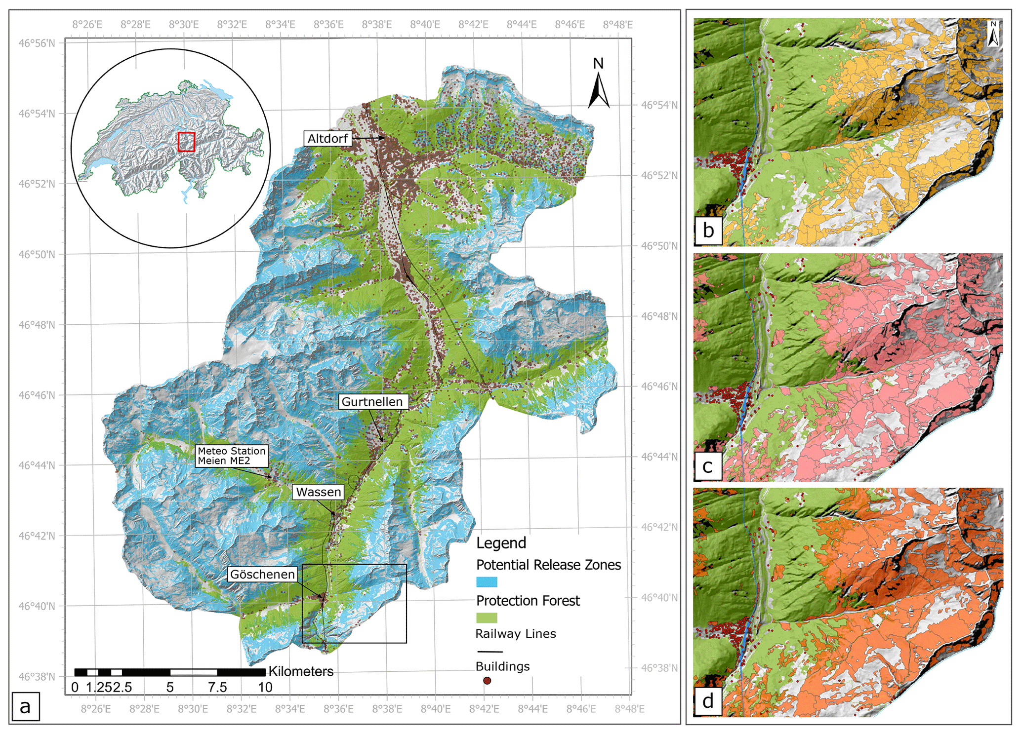
Figure 4 (a) Overview of the study area with the automatically generated protection forest layer in green and the area of potential avalanche release in blue. (b–d) Automatically generated individual potential avalanche release areas (b) for a 30-year return period, (c) for a 100-year return period and (d) for a 300-year return period. Map base data source: Swiss Federal Office of Topography.

2.3.2 Creation of the avalanche protection forest layer

Forest influences the snowpack structure by interception and changes in the micro-climate. An increased topographic ground surface roughness in forests and irregular layers in the snowpack prevent avalanche formation. In some cases dense forests are even able to stop movement of small avalanches due to higher friction in the flow and the avalanche run-out zone (Schneebeli and Bebi, 2004; Bebi et al., 2009; Teich et al., 2012; Brožová et al., 2021). To take forest cover into account for hazard mapping, we used the algorithm developed by Bebi et al. (2021) and introduced by Bühler et al. (2022) to identify protective forest in the study area (Fig. 4). The algorithm developed by Bebi et al. is based on a database of 150 forest avalanches and yields a logistic regression model, taking into account the parameter's slope gradient, degree of forest cover and widths of gaps between trees. Together with a vegetation height model and a high-resolution elevation model, a general logistic regression model was used to calculate forest conditions (Bebi et al., 2021) to define if avalanches can occur or not. The thus derived protective forest layer was calculated for frequent (return periods < 100 years) and extreme scenarios (return period > 100 years). The protection forest model is improved and extended by a “shrub forest” layer (Weber et al., 2020) and a ground roughness layer. Since shrub forest also has a protective function against avalanche release, the existing protective forest layer was expanded with a shrub forest component. Compared to normal protection forest, shrub forest has a reduced protection capacity, which is taken into account. This is a significant improvement over previous protective forest layers in which shrub forest was not taken into account. In this study, in a frequent scenario with a 30-year return period, shrub forest prevents avalanche release, whereas in the large avalanche scenarios with 100 or 300-year return periods, shrub forest no longer has any influence. The ground roughness layer classifies rough ground to mitigate avalanche release to a certain extent. The implemented ground roughness is taken into account for the protective forest layer calculation in frequent avalanche scenarios. This procedure results in a binary protection forest layer (green forest layer in Fig. 4) that divides the area of investigation into areas with and without protection forest. With a forest layer generated this way, it is assumed for the large-scale avalanche mapping process that an avalanche release in the forest is not possible (Bühler et al., 2018b). Further details on the algorithm are delivered by Bebi et al. (2021).

Terrain models used for the selection of the release areas no longer contain buildings or infrastructure. Thus, the algorithm can designate release areas in places where there is actually infrastructure. Of course the formation of avalanches is also altered by infrastructures, which can completely prevent avalanche formation or subdivide release areas into smaller ones, e.g., a road cutting through a steep slope. Therefore, infrastructure such as roads, railway lines and buildings are also added to the binary layer as being objects that prevent avalanche release.

2.3.3 Generation of automated avalanche release areas

Identifying the potential avalanche release areas is a crucial hazard assessment. Individual expert analysis and manual release area selection is no longer efficient for a large-scale application. We therefore use an automated approach introduced by Maggioni and Gruber (2003) and further developed by Bühler et al. (2013), Bühler et al. (2018b) and Veitinger et al. (2016), applied to large scales by Bühler et al. (2022).

This approach is based on a terrain analysis in a GIS and the “object based image classification” (OBIA) method (Blaschke, 2010) to delineate the individual release polygons, which serve as an input for the large-scale avalanche hazard indication modeling (Bühler et al., 2013, 2018b). The algorithm analyses the slope geometry and identifies all possible potential avalanche release zones automatically for a given set of input data. With the fracture depth derived from the snow depths (Sect. 2.3.1) and the area of the release zones, as well as applying the corresponding correction factors, the volume for each release area could be determined. With the automated processing, the single-potential avalanche release areas are mapped and classified into four release area size classes: large (release volume >60 000 m³), medium (25 000–60 000 m³), small (5000–25 000 m³) and tiny (<5000 m³). Depending on these release volumes, different friction parameters are assigned to the associated avalanche for the subsequent simulation. These friction parameters μ (basal friction) and ξ (turbulent friction) are assigned according to the RAMMS standard modeling procedure (Christen et al., 2010), which is standard for hazard mapping in Switzerland.

2.3.4 Large-scale avalanche hazard indication mapping with RAMMS::LSHIM

We used RAMMS::LSHIM (Rapid Mass Movement Simulation::Large-Scale Hazard Indication Mapping), which is a special version of the base module of RAMMS::AVALANCHE, a numerical avalanche simulation model capable of simulating avalanches in complex topography (Christen et al., 2010). RAMMS::AVALANCHE is based on an efficient second-order numerical solution of the depth-averaged avalanche dynamics equations and the two-parameter Voellmy model (Voellmy, 1955) and has been calibrated with numerous observed avalanches, such as those at the SLF test site in Vallée la Sionne (Arbaz, Valais, western Swiss Alps). For the simulations, a three-dimensional digital terrain model, with a spatial resolution of 10 m; the generated potential release areas; and the avalanche fracture depth (Table 1) served as inputs to calculate avalanche volumes, flow velocities, flow heights and impact pressures for 40 000 individual avalanches. This was done for all three scenarios. Each avalanche was assigned to a release zone and registered individually, which allowed us to allocate each avalanche with its pressure to a return period, to be used subsequently in a risk analysis.

For avalanche release volumes <25 000 m³, the binary forest layer is considered for the flow simulations with the assigned friction parameters μ (mu: basal friction) and ξ (xi: turbulent friction). Values of μ=0.020 and ξ=400 were assigned for the simulations in RAMMS::LSHIM because protective forest has a strong influence on friction during avalanche runout in frequent scenarios with smaller avalanche volumes. For avalanche release areas with volumes >25 000 m³, the influence of the protective forest is neglected, since the energy generated during the flow process mostly destroys the protective forest, which thus hardly has any effect on the size of the affected area in the run-out zone (Bartelt et al., 2017). In the extreme scenarios, the potential release zones with avalanche volumes <25 000 m³ are simulated with forest influence. In the frequent scenarios, on the other hand, the potential release areas with avalanche volumes >25 000 m³ are simulated without forest influence. This is part of an extended set of algorithms for automatic release area identification (Bühler et al., 2018b, a, 2022) and the standard friction parameter set, which is commonly used in practice (Christen et al., 2010; Gruber and Margreth, 2001). For a detailed description of the RAMMS::AVALANCHE application in RAMMS:LSHIM, see Bühler et al. (2018b).

Figure 5 shows the resulting large-scale hazard indication map and, in detail, how the individual scenarios were simulated, taking into account protection forest.

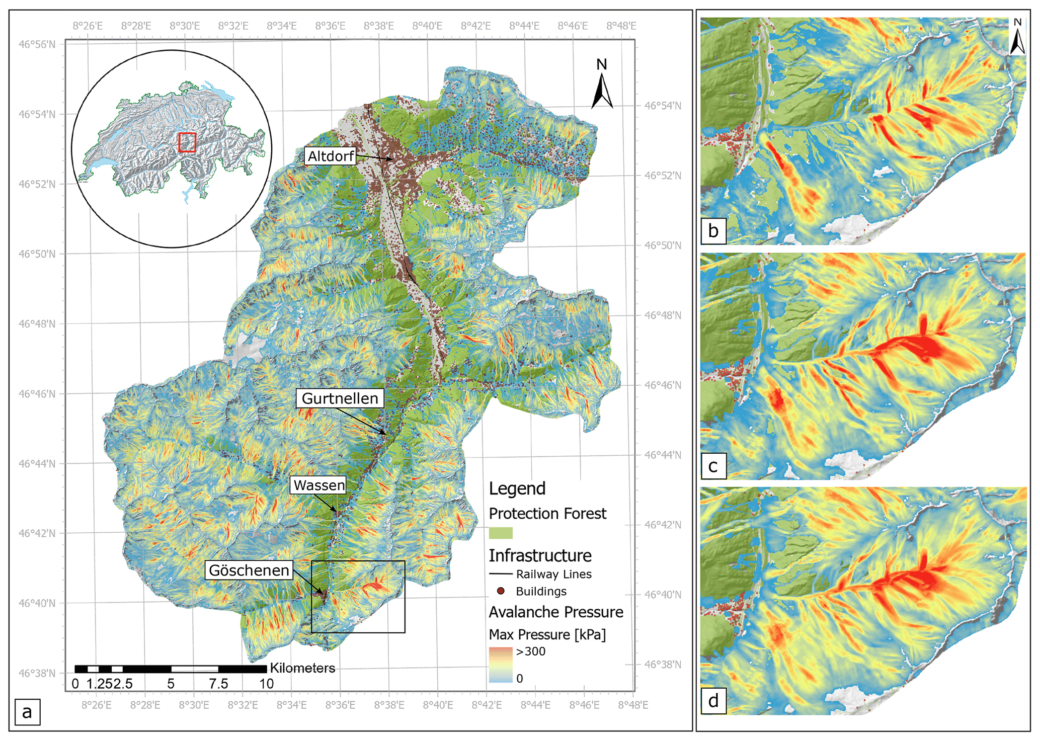
Figure 5 (a) Project area with results of the large-scale avalanche simulation, pressure in (kPa), (b) detail of the simulation for the frequent scenario, corresponding to a 30-year return period, (c) detail of the simulation for the large scenario, corresponding to a 100-year return period, (d) detail of the simulation for the extreme scenario, corresponding to a 300-year return period. Map base data source: Swiss Federal Office of Topography.

2.4 Exposure

2.4.1 EconoMe

EconoMe is an online tool for the evaluation of the effectiveness and economic efficiency of mitigation measures against natural hazards (Bründl et al., 2016). It provides a sophisticated methodology for risk analysis and the evaluation of the cost–benefit ratio of protective measures and is used by private companies and cantonal and federal authorities for decision support regarding the distribution of subsidies. All values used for this study were generated using the EconoMe methodology and are described in Sect. 2.4.2 and listed in Table 2.

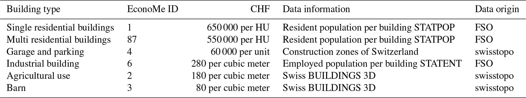
Table 2 Overview of the base data used for the creation of the monetary building layer, definition of monetary values of building types; abbreviations: HU is housing unit, FSO is Swiss Federal Statistical Office (FSO, 2019), swisstopo is Swiss Federal Office of Topography and ID is EconoMe object identification number.

2.4.2 Generation of high-resolution exposure point datasets with monetary values

Four main datasets were used to determine monetary values: (1) STATPOP, statistical population data which provide information on the number of building inhabitants; (2) STATENT, statistical data specifying which buildings are used for economic purposes; (3) construction zones Switzerland, providing information about settlement areas or agricultural zones; and (4) a 3D dataset of all Swiss buildings, including the volume of individual objects. To allow a high performance in risk calculation and a broad applicability, buildings in the exposure data frame are considered as point objects located in the center of a building polygon. Using these four datasets, an exposure point layer was created according to the guidelines for creating risk overviews (FOEN, 2020) as described in the following.

The GIS layer with assigned monetary values was created for 13 304 individual objects. To generate this monetary building layer, objects needed to be classified using the above-mentioned datasets, also listed in Table 2. The classification was carried out by plotting the statistical data STATPOP and STATENT on a 2D building layer. The monetary values of buildings were assigned according to the building types also listed in Table 2. According to EconoMe standards, the average number of persons in one housing unit (= HU) was assigned as 2.24 persons per unit (FOEN, 2021). By using STATPOP, we identified the number of persons living in each building and determined the number of housing units rounded to the next smaller number. When the number of persons per object was below 2.5, the object was classified as a single residential building; when the number of persons per object was higher than 2.5, it was classified as a multi-residential building. Based on the number of HU, monetary values could be assigned to the objects as listed in Table 2.

Since there is no comprehensive data available for evaluating the value of companies and buildings, the STATENT dataset was used. These data provide building coordinates for each registered company in Switzerland. If one or more STATENT data point plots on the location of a building, this building was classified as a business building. The value corresponds to the volume of the building (FOEN, 2021), which was taken from the Swissbuildings3D dataset, yielding a value of CHF 280 per cubic meter volume. For objects with the combined usage “business and living”, on which both the STATENT and STATPOP data points apply, the number of residential units was taken for the assignment of the monetary value, as these have higher value.

Buildings located within the Swiss construction zone plan with no inhabitants and a volume of less than 100 m³ were classified as uninhabited outbuildings, with a value of CHF 60 000 per unit (garages and parking lots including vehicles). Uninhabited outbuildings with a volume greater than 100 m³ were classified as economically used buildings, and their value was determined by the volume.

Buildings located outside the Swiss construction zone plan with a volume less than 100 m³ were classified as agricultural outbuildings (barns), with a value of CHF 80 per cubic meter. If their volume is greater than 100 m³, they were classified as agricultural main buildings with a value of CHF 180 per cubic meter (FOEN, 2020). This method allowed the creation of an exposure data layer, shown in Fig. 6, with a monetary value for each individual building.

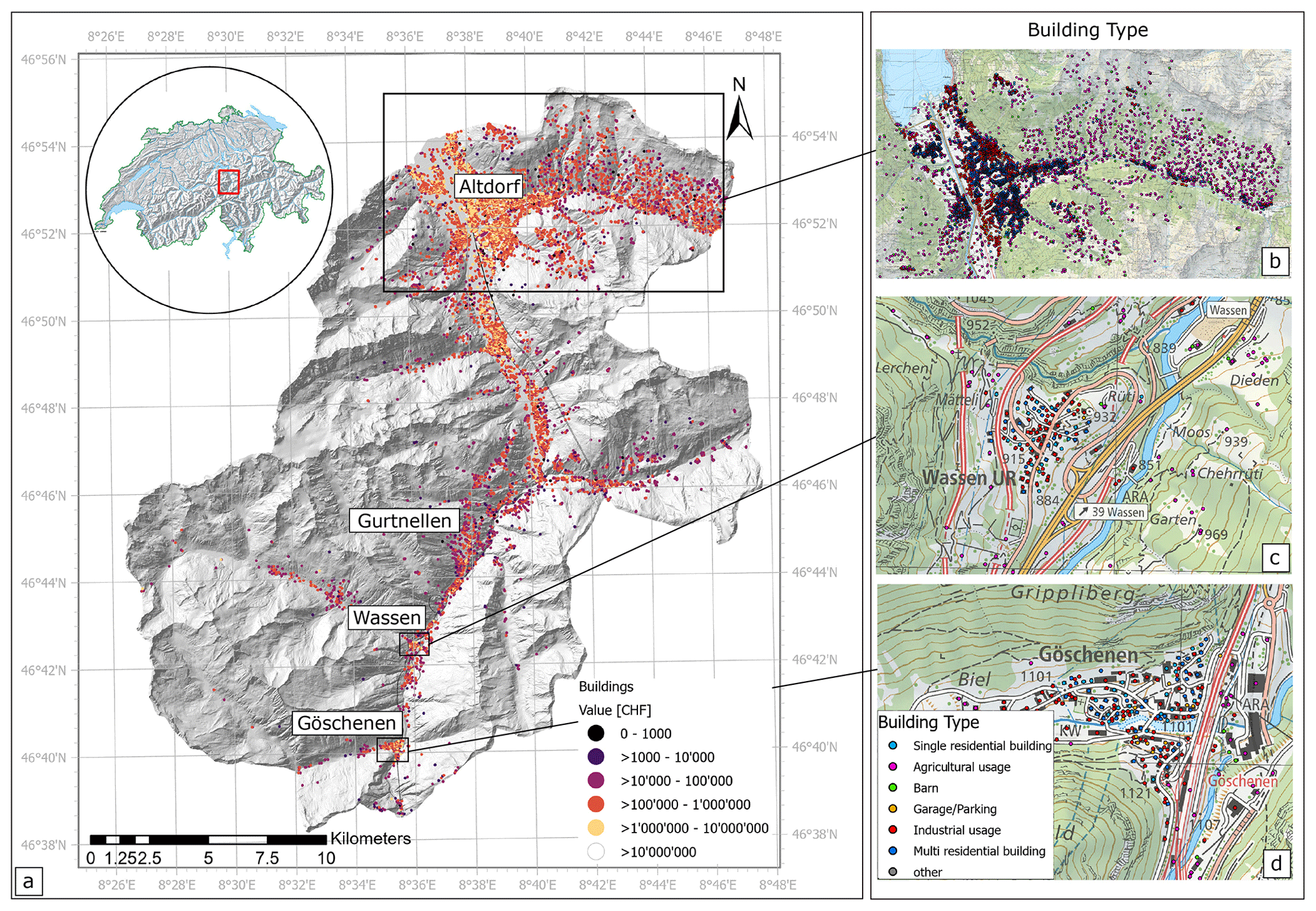
Figure 6 (a) Spatial distribution of exposed monetary values in the project area. (b) Detail section, different building types matching actual buildings on the map (Map source: Swiss Federal Office of Topography, modified map).

2.5 Vulnerability

Avalanche impact functions

The extent to which an object is damaged by a hazard is referred to as the “hazard impact” or “impact”. We determined the impact by avalanches using so called “impact functions”, which are equivalent to “vulnerability functions” or “damage functions”, as defined in the CLIMADA methodology (Aznar-Siguan and Bresch, 2019), which express the damage an object suffers at a certain avalanche intensity (pressure in kPa). These functions are based on values in EconoMe (FOEN, 2021). These step functions originate from the standardized hazard mapping procedure in Switzerland, where continuous avalanche impact pressures p are divided into three pressure classes ($\mathrm{0}<p\le \mathrm{3}$ kPa, $\mathrm{3}<p\le \mathrm{30}$ kPa and p>30 kPa). These step functions follow the Swiss standard (FOEN, 2021) and are based on an evaluation of building damages and expert judgment. According to construction type, objects show varying damage susceptibility to avalanche impact pressure. We defined impact functions with three components for each object type and combined them into a impact function set to describe the following avalanche impacts:

• the mean damage degree (MDD), expressing the mean percentage of damage an object suffers under a certain avalanche impact pressure, expressed in kPa;

• the percentage of affected assets (PAA) in the hazard zone, where buildings exposed to avalanche impact pressure that suffer damage is assumed to be 100 %;

• the mean damage ratio (MDR) at a certain pressure, in this study mean damage ratio is equal to mean damage degree.

The mean damage ratio is a standard vulnerability unit. It is described as the ratio between the damage of affected objects and the total value of all objects exposed to the hazard. The application of these standard vulnerability components to avalanches is a special case. We assume in this framework that all objects exposed to a certain avalanche impact pressure also suffer damage according to the mean damage degree thresholds. Therefore, we set the mean damage ratio as equal to the mean damage degree.

2.6 Uncertainty and sensitivity analysis

The uncertainty analysis describes the variability of the output of the model, given a range of the input parameters, while a sensitivity analysis describes how a certain uncertainty in the model can be assigned to a certain input parameter (Saltelli et al., 2019; Saltelli, 2002; Kropf et al., 2022). In this study, the model outputs of interest are the average annual impact and aggregated overall exposure points for hazards with different return periods (cf. Sect. 2.3.1). In general, it is not possible to consider the uncertainty of all input parameters in a model such as CLIMADA. For this study, we focus on the total exposure value (building value), the mean damage degree thresholds of the impact functions (vulnerability) and the uncertainty of the intensity of the avalanches (impact pressure; Sect. 2.3), as discussed in details in Sect. 2.6.1.

2.6.1 Uncertainty analysis

Since the values of the exposure were determined with the generalized value assignment procedure introduced by FOEN (2020), it is clear that these can deviate from real life building values. The FOEN (Federal Office for the Environment) method provides an estimation of a building value at a large scale but cannot resolve the differences in value of similar building types. To account for the potentially large fluctuation in asset value, an uncertainty of ±20 % of the total exposures value is assumed. In other words, for each run of the uncertainty sampling, all the assets' values are multiplied with a value “ET”, uniformly sampled from [0.8,1.2].

Industrial and residential buildings are the most costly building types. The steps of the impact functions for residential buildings and industrial differ by 40 %. To account for a large degree of uncertainties, this value of the step jump in the function was taken as the possible uncertainty range. For agricultural buildings or outbuildings, this value can be even higher, as they often have a relatively simple construction. But due to their lower value they play a less important role. To define a “standard case” in our analysis, we consider the function steps of industrial or residential buildings as the variability range. Therefore, for the mean damage degree of the impact function a value range of ±40 % was taken for the uncertainty analyses (cf. Table 3).

Table 3 Uncertainty ranges of the chosen input parameters for the risk assessment.

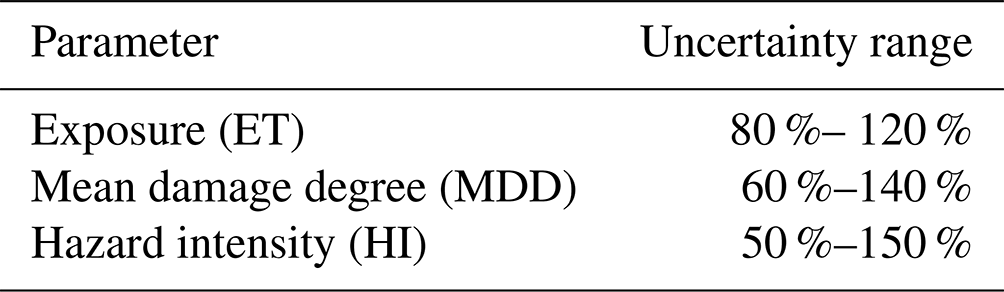
To define a range for the hazard intensity uncertainty analysis, we refer to data recorded in experiments at the Vallée de la Sionne test site. Sovilla et al. (2008a, b) measured the impact pressure of dry, wet or mixed avalanches with different flow regimes on obstacles. In our simulations, we only simulated “dry avalanches”, which mostly have velocities higher than 10 m s⁻¹. Pressure values of avalanches measured by Sovilla et al. show avalanche impact pressures ranging between 200 and 700 kPa (Sovilla et al., 2008a). An extrapolation of the dataset would yield maximum pressures of about 1000 kPa, which corresponds to the data obtained in our simulations shown in Fig. 5. The average pressure of the measurements would be around 600 kPa. Therefore, we assumed an uncertainty range of ±50 % for avalanche impact pressure (cf. Table 3). The obtained samples are illustrated in the Appendix, Sect. A, in Fig. A1.

2.6.2 Sensitivity analysis

The sensitivity analysis determines which input parameter's uncertainty has the strongest influence on the model output uncertainties (Saltelli et al., 2019). In this study, we used the Sobol sensitivity indices (Sobol, 1993, 2001) as implemented in CLIMADA (Kropf et al., 2022), which can be computed from the same Sobol sequence as used for the uncertainty analysis (cf. Fig. A1, Appendix Sect. A). The Sobol sensitivity analysis method is a popular, variance-based method that quantifies the contribution of the variance of one or two parameters to the unconditional variance of a model output (Nossent et al., 2011). It is expressed as the Sobol sensitivity index. After the distribution of the impact metrics has been computed for all samples (see Sect. 3.2), the sensitivity index for the each metric was computed. We considered the first-order Sobol index S1 that describes the contribution of a single model input to the output variance. This index therefore provides information on the most influential parameter, with reference to its system (model).

3 Results

3.1 Risk maps

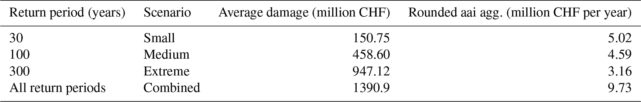
With CLIMADA and all the risk components described above, we are able to express risk measures such as the expected annual impact and the average annual impact for all objects in the case study region, taking into account different synthetic hazard scenarios. Figure 8a–d show how different hazard scenarios affect single objects located in the hazardous area. Figure 8a depicts the risk pattern of the entire study area. Further risk overviews for the 30-, 100- and 300-year return period scenarios can be found in the Appendix, Sect. A, Fig. A2. Figure 8b shows a detail of the risk map of the Göschenen area with a 30-year return period scenario and the Rientalbach avalanche path in order to compare it with the 100-year return period in panel c and the 300-year return period scenario in panel d. The colored dots represent the expected annual impact corresponding to a 30-year return period. As shown in Table 4, the aggregated average annual impact ranges from CHF 3.2 million to 5.02 million per year, depending on the scenario. In the aggregated scenario, it reaches up to CHF 9.73 million. In the detail panels of Fig. 8b–d, it can be seen that with increasing return period the area affected by avalanches gets larger, and the number of objects at risk increases. Nevertheless, the objects in the hazard zone show lower risks in the higher return periods. This clearly shows the influence of return period on risk. The less likely an event is to occur, the lower the associated risks for the individual object. The aspect of more exposed objects at risk is expressed by the aggregated average annual impact over the entire project area.

Table 4 Overview of the average damage and the rounded aggregated average annual impacts (aai agg.) for each of the avalanche scenarios and all hazard scenarios combined. The rounded aggregated average annual impact corresponds to the overall risk of the entire region.

As depicted in the risk maps in Figs. 8a and A2 of the Appendix, it is evident that in all scenarios the most densely populated areas (see Fig. 6) in the main valleys do not represent the greatest risk accumulations. Hotspots are located on the slopes of the main Reuss Valley near Wassen, further north in Gurtnellen and in the side valleys of Wassen near Meien. In these areas, mountainous terrain with a high number of avalanche flow paths and a denser number of buildings overlaps. There, the exposed objects are mostly agricultural buildings. According to our method, the value of these buildings depend on their volume. Agricultural buildings can be large in volume but also very vulnerable to destruction by avalanches (see Fig. 7) due to their construction type. This leads to high impacts at these locations, as shown in Fig. 8. However, there are also a few multi-residential buildings in the endangered areas. If these buildings are at high risk, they appear on the map as dark dots. The largest accumulations of buildings at risk are found on the southeast to southwest facing slopes east of Altdorf. The identification of such hotspots can play a crucial role in a decision making process, as discussed in Sect. 5.

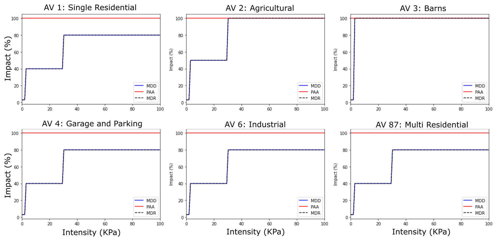
Figure 7 Impact functions showing the mean damage degree (MDD) of different building types exposed to a certain intensity (the mean avalanche impact pressure); percentage of affected assets (PAA) is 100 %.

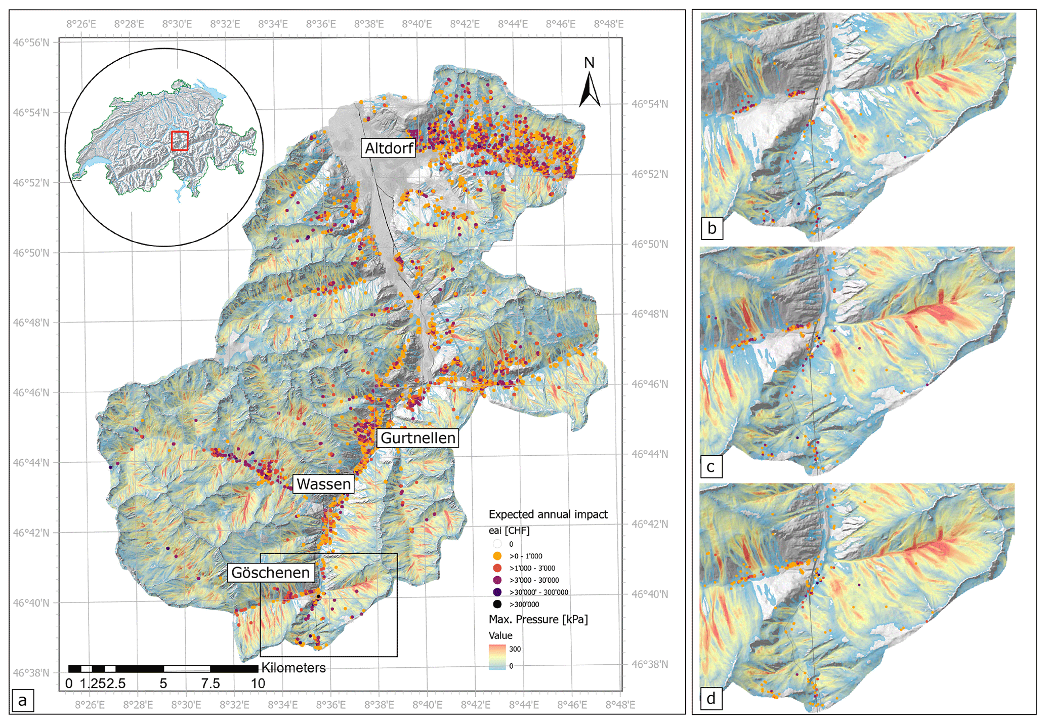
Figure 8 Risk maps: overview of the spatial distribution of expected annual impact for individual objects at the four different avalanche scenarios (a) overview of all hazard scenarios combined, (b) detail Göschenen 30-year return period, (c) detail Göschenen 100-year return period and (d) detail Göschenen 300-year return period. Basemap source: Swiss Federal Office of Topography, modified surface model.

3.2 Impacts, uncertainty ranges and sensitivity analyses

For the first event set with a 30-year return period (Fig. 9 in blue), the maximum count of sample histogram bars plotted between CHF 3.4 million and 5.6 million. This illustrates that the annual impact severity for a hazard with a frequency of $\mathrm{1}/\mathrm{30}$ is likely to lie in this range. The non-aggregated average annual impact values generally range from CHF 2.0 million to 9.0 million. This implies a wide dispersion of risk, yet reflects the broad distribution of the exposed monetary values in the hazard area. Building values range from less than CHF 1000 to maximum building values of CHF 78 million. The sample size was 8000 generated samples for each parameter, and the impact was calculated for each of these samples. The histogram is not normally distributed, it shows a right-skewed distribution with an average impact value of CHF 4.87 million and with an SD of CHF 1.34 million. Taking into account all uncertainty ranges discussed above, it is very likely that the annual risk for a 30-year return period scenario across the entire region will be in the range CHF 3.4 million to 5.6 million per year.

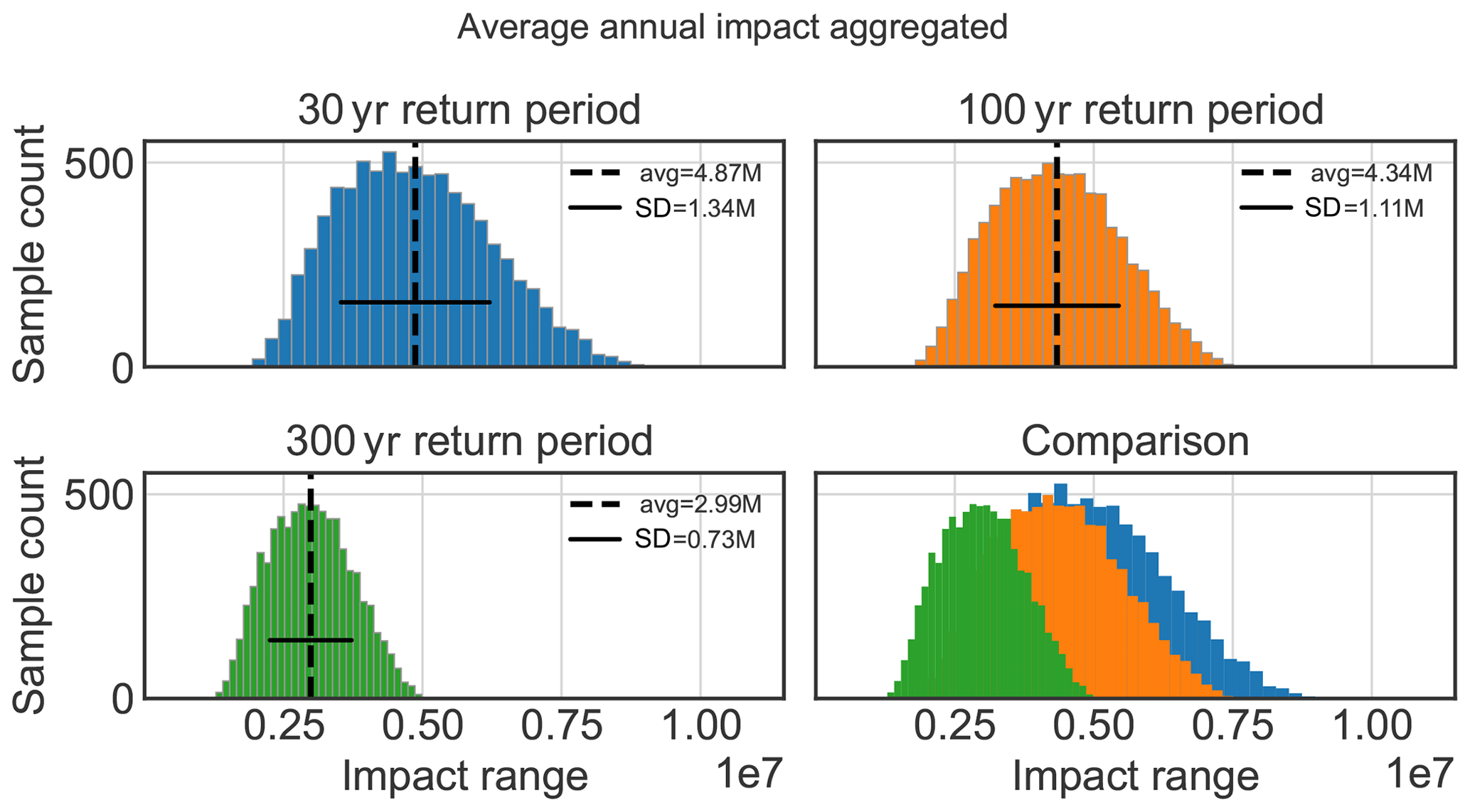
Figure 9 Histograms of the calculated distribution of the aggregated average annual impact values from the return period scenarios in CHF: blue is 30, orange is 100 and green is 300 year, calculated for 8000 randomly pulled samples within defined uncertainty ranges (Table 3; avg is average, SD is standard deviation).

The situation is slightly different for the scenario with a 100-year return period (Fig. 9 in orange): despite higher avalanche impact pressures, the risk is lower, with a lower variance. Taking into account the uncertainties, the possible annual impact in the project area is between CHF 2.9 million and 5.4 million. The distribution extends almost over the same range as the 30-year return period scenario (Fig. 9 “Comparison”), but the 30-year scenario shows a sightly higher sample count in a higher impact range. The average annual impact across all values inside the chosen uncertainty range for the 100-year return period scenario is CHF 4.34 million, with an SD of CHF 1.11 million. The histogram for the 100-year return period also shows a right-skewed distribution, and compared to the 30-year return period distribution it is almost equally distributed.

Looking at the distribution of the 300-year return period scenario, and in the comparison (Fig. 9 in green), we see that the average value of the annual impact is CHF 2.99 million, with an SD of CHF 0.73 million; the risk is significantly lower than in the 30-year return period scenario and also lower than in the 100-year return period scenario. The highest sample count is in a variability range of CHF 2.5 million and 3.6 million. The total damage caused by avalanches in the 30-year return period scenario would be approx. CHF 150.8 million; for the 100-year return period scenario, CHF 458.6 million; and approximately CHF 947.1 million for the 300-year return period scenario.

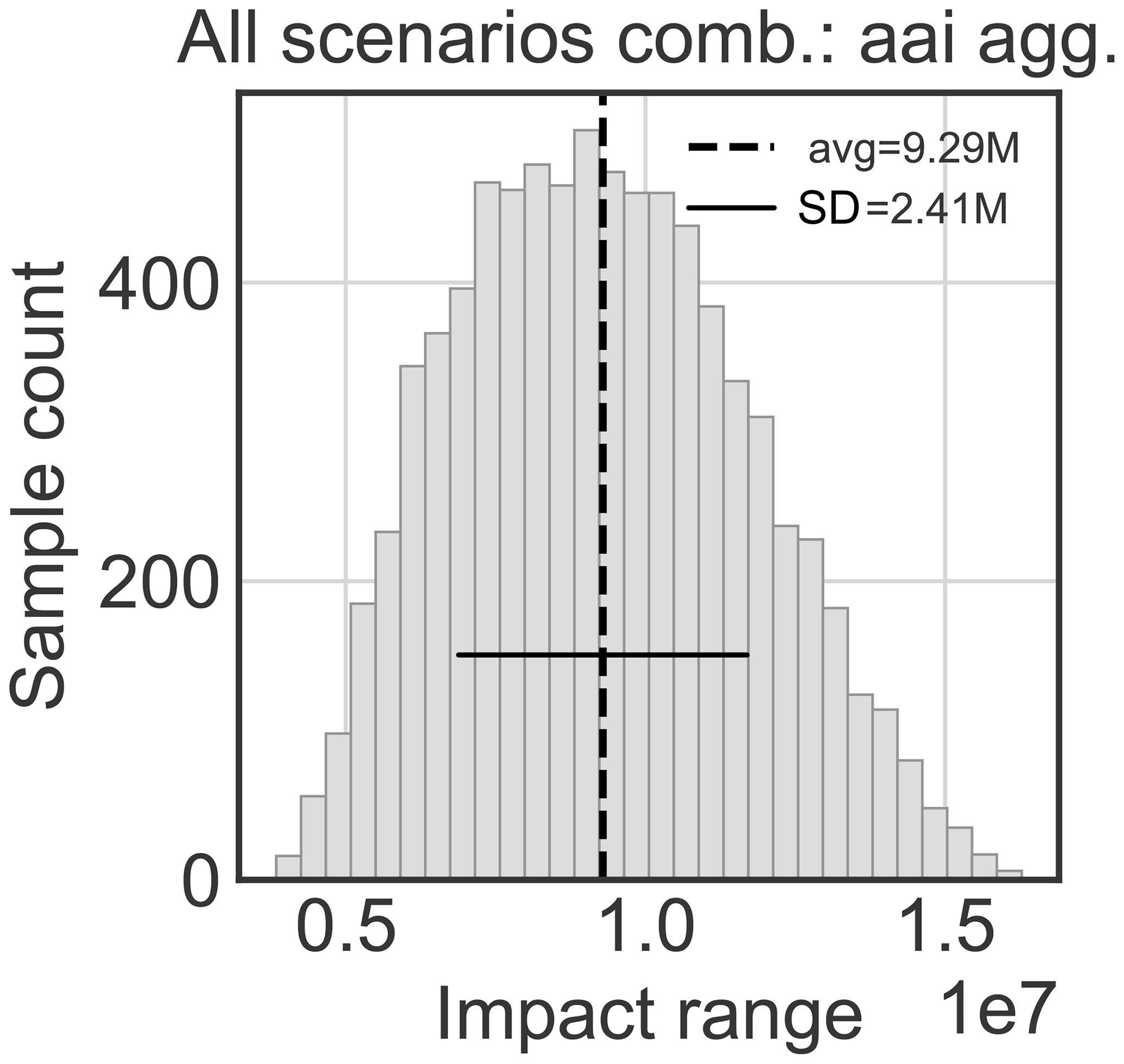
In the combined scenario in Fig. 10, we see a significantly higher impact range of CHF 7.0 million to 11.5 million, with an average value of CHF 9.29 million and an SD of CHF 2.41 million. This shows the high influence of the return period in the calculation of the risk. The risk of a 30-year return period scenario is therefore significantly greater than that of a 300-year scenario.

Figure 10 Average annual impact aggregated of all hazard scenarios in CHF combined and summed over the entire case study area. Calculated for 8000 randomly pulled samples within defined uncertainty ranges (Table 3; avg is average, SD is standard deviation).

3.3 Damage-frequency curve

The damage-frequency curves show the calculated impacts and their uncertainty distributions for all considered scenarios in relation to the return period. The average damage for the three considered scenarios shown in the risk overviews is depicted in Fig. 11a. To incorporate a comparison of the designated return period scenarios with the results of the uncertainty analysis, we calculated the 95th and 5th percentile of all damages of the three scenarios of the uncertainty analysis. Thus, for the confidence interval calculation, 8000 values were available from the uncertainty analyses for each of the three return periods (30, 100, 300 year). As shown in Table 4 and Fig. 11 the damage for a frequent (30-year return period) scenario is about CHF 150.8 million, with a variation from CHF 151–216 million (5th–95th percentile). In the 100-year return period scenario the average damage is CHF 458.6 million, with a variation (5th–95th percentile) of about CHF 262–625 million. The higher the scenario, the more objects are affected and the larger are the uncertainties expressed in monetary terms. The 300-year scenario shows an average damage of CHF 947.1 million, with a large uncertainty range from CHF 548 million–1.27 billion (5th–95th percentile). The variability of the calculated damages stemming from uncertainty can be seen in Fig. 11a and b. The median value (black line in the boxplots), calculated from all values of the uncertainty margin of the scenarios, is compared with the average damage of the three designated scenarios (see Table 4; displayed as a black square in Fig. 11b). Figure 11b shows that the average damage values of the three single scenarios are close to the median values of the box plots calculated from all values including the uncertainty margin. It demonstrates that the original calculations for the single damage values (from the three scenarios) are of good quality. Whether the interpolated damages from the scenarios that were not calculated (e.g., 0–30, 30–100 or 100–300 year) in this study are in a linear relation to the calculated damage is a rough assumption. Nevertheless, this curve can be used to infer approximate dimensions of the damage to be expected in other return periods, taking into account various uncertainties.

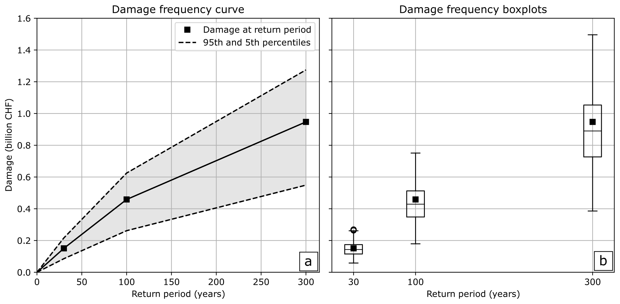
Figure 11 (a) Damage-frequency curve showing the calculated damage at a certain return period, with the 95th percentile of all damages calculated within the defined uncertainty ranges. (b) Boxplots of the three scenarios depicting all calculated damages of all uncertainty samples (black square is average damage (without return period) of the three scenarios). The boxes extend from Q1, the first quartile, to Q3, the third quartile, of the impacts at return period; the median is depicted as a line. The whisker lines enhance from the box by 1.5× the interquartile range. Points are data exceeding the end of the whiskers.

Input parameter sensitivity analysis

The first-order sensitivity index S1 identifies which parameter impacts the aggregated average annual impact most. Figure 12a–c show that the mean damage degree plays the most important role in this model for all scenarios. For the scenario with a return period of 30 years and the scenario with a return period of 100 years, the exposure and the hazard intensity seem to be almost equal. In the extreme scenario with a 300-year return period, substantially more objects are affected (see Fig. 8), and the exposure plays a slightly more important role here. The sensitivity index of the hazard intensity in the 30- and 100-year return period scenarios (Fig. 12a and b) is slightly higher than the S1 of the hazard intensity in the 300-year return period scenario in Fig. 12c. It is thus scenario-dependent whether the hazard intensity or the exposure have more influence. However, in all scenarios the mean damage degree defined by the impact functions is the most relevant parameter. For the combined hazard scenario (Fig. 12d) it is similar to the 300-year return period scenario. Both the exposure and the hazard intensity have almost the same high sensitivity index, but again the mean damage degree is more decisive.

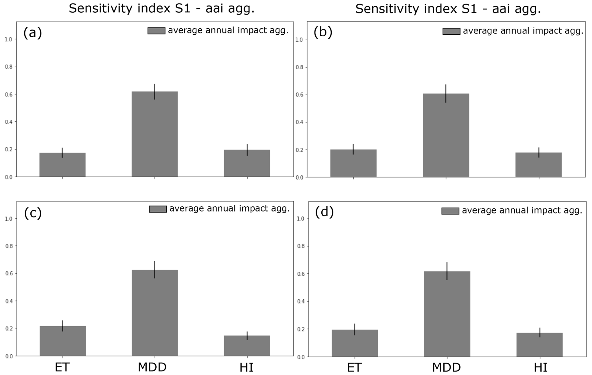
Figure 12 S1 is the first-order sensitivity index and its effect on the average annual aggregated impact value (a) frequent hazard scenario, 30-year return period (b) medium hazard scenario, 100-year return period (c) extreme hazard scenario and 300-year return period (d) overall combined. ET is exposure, MDD is mean damage degree and HI is hazard intensity.

4 Discussion

4.1 Risk maps and hotspots

As shown in Fig. 8a, the biggest accumulation of avalanche prone objects is on the southwest facing slopes east of Altdorf. One explanation for this hotspot is the high number of agricultural buildings and a few residential buildings on very steep, avalanche-prone, open slopes. If one compares risk maps of Figs. 8a and A2, it can be seen that depending on the scenario the expected annual impact is strongly variable, indicated by the different colors; also, the numbers of objects affected is different. Although the number of affected buildings is higher in the large 100- and 300-year scenarios, the risk for the individual objects is higher in the 30-year return period scenarios. The avalanche extents are larger, and buildings experience similar, or slightly higher, avalanche impact pressures due to larger avalanche volumes in the 100- and 300-year scenario. The lower risks are mostly driven by the influence of the low hazard frequency (high return period), which substantially influences the risk. The aggregated annual impact (overall risk) allows a comparison across the entire region and all scenario.

From a risk management perspective, one could conclude that mitigation measures reducing the damage in the 30-year and/or the 100-year return period scenario would be very effective for reducing the overall risk.

4.2 Limitations

4.2.1 Large-scale avalanche hazard mapping

The proposed approach has a fast and powerful applicability, which allows us to map potential release areas over very large areas, where only the computational capacity and the computation time define the limits of its application. This method is applicable worldwide and requires a small number of input data, making it one of the most unique and powerful tools for large-scale hazard mapping. We consider that the advantages of the large-scale applicability and the preciseness of the results meet the goals of our study.

Compared to a detailed hazard assessment, there are some limitations (Bühler et al., 2022). In such a multi-step process, avalanche release areas are manually identified by experts performing a detailed terrain assessment, including an evaluation of protection forests, which is used as input for a numerical modeling of avalanche run out (Rudolf-Miklau et al., 2014). In our approach, potential release areas are only identified on the basis of terrain and scenario characteristics. This is an approximation, as actual avalanche release zones may vary in shape and size in nature. However, a validation of this algorithm carried out by Bühler and colleagues showed that results are in good agreement with avalanche observed in the terrain (Bühler et al., 2018b).

The definition of the protection forest was based on datasets compiled at a specific point in time in the past (2020) using remote sensing methods. However, with the effects of extreme windstorms, bark beetle infestations or consequences of climate change (e.g., dry periods), the forest structure can change rapidly (Brožová et al., 2020, 2021). A detailed consideration of these effects and an expert evaluation of the protective function of a particular forest (Bebi et al., 2021) is not applicable for large-scale applications and cannot be imperative for the preparation of risk overviews.

Using 3 d snow depth from a single weather station results in uncertainties for both the scenario definition and fracture depth. Both have a direct effect on the avalanche volume and subsequently on the extent of avalanche runout. The longer the time series, the more extreme snowfall events would have been recorded. However, the time series of 66 years used in our study is common practice for avalanche hazard assessment. The time series available are comparatively long, and longer series were not available either. However, this involves bigger uncertainties for estimation of fracture depths at high return periods. As can be seen in Fig. 3, the GEV method results in ±30 cm for a 100-year return period and ±50 cm for a 300-year return period, and the Gumbel method results in ±20 cm for the 100-year return period and ±25 cm uncertainties for the 300-year return period. Due to the 66-year record period, it can be assumed that the estimate of 3 d snow depth increase for a 30-year scenario contains lower uncertainties (±15 cm). This consideration of uncertainties does not take into account local wind effects that can arise because of topography changes at ridges and the back of mountains that significantly influence snow deposition in the release areas. These effects can lead to a high variability of the snow pack in the release zones. However, these local conditions cannot be taken into account in such large-scale applications. Only a wind load factor (30–50 cm) depending on the scenario size was added. Without detailed wind and snow deposition studies, this uncertainty in the modeling process is hard to quantify and has to be accepted.

Further, the topography and the assigned friction parameters play the most important role in the run-out flow simulation of an avalanche. For single slope assessments, different parameters (μ and ξ) would be assigned for each change in the flow cross-section (gully, channel or open slope), and thus, more precise results could be obtained. This leads to a less differentiated hazard pattern compared to a single slope approach in the avalanche run-out zone. Another effect that includes uncertainties is that all theoretically possible potential release areas are simulated with our model. In reality, a more differentiated picture of avalanches would result for each catchment zone, in which some release areas produce an avalanche and others do not. Over an entire catchment area, this leads to an overestimation of avalanche risk because too many objects are affected. This effect is not uniform for each slope aspect or catchment area. As far as we know, there are no studies on the release probability of avalanches that can be applied to large scales to represent an actual natural avalanche release scenario in a model. The advantage of our approach is, however, that all potential avalanche release areas that have the required geometrical properties for avalanche formation are actually covered in the simulation and taken into account for risk assessment. Here, the need for further research is identified to design probabilistic avalanche sets to cover real life avalanche release scenarios. In our risk analysis, each individual avalanche is treated as an individual, independent event, and the resulting damage is averaged out over all events impacting an object.

4.2.2 Building impacts and avalanche risk mapping

In this paper, we identify the monetary avalanche risk for buildings at a large scale. To do this, some generalizations have to be made, which leads to certain limitations in the level of detail.

The impact functions define the damage rate in steps and pressure classes. Actual damage does not always depend on these classes. If an avalanche hits an object, it is important at what angle the building is oriented in relation to the flow direction of the avalanche, what the specific flow regime is as well as how high the avalanche flows (Kyburz et al., 2018), or whether the building has structural weaknesses (e.g., windows or doors) exposed to the avalanche flow. Even though the impact step function was derived from expert assessments and damage surveys of avalanche incidents, it is unlikely that damage occurs according to these steps or is linear to the avalanche impact pressure – depending strongly on the individual situation. Even minor damage to the foundations of a house can lead to total damage and reconstruction. In our method, all these details cannot be taken into account. To ensure the performance of our approach, we generalize. We consider buildings as point objects with a generalized vulnerability. When using central points in building polygons, we naturally underestimate the influence of the actual three-dimensional building size in the avalanche flow. Small buildings are therefore equally considered as large buildings. Nevertheless, this approach allows a simple and performative applicability and an efficient large-scale approach but introduces inaccuracies in detail. However, we try to address the framework of these uncertainties by means of an overall uncertainty analysis.

Further, our method of the avalanche impact calculation does not take into account the temporal effects of the hazard. In reality, the first avalanche that destroys an object completely “prevents” its destruction by further events. After many minor avalanches have occurred in the same catchment area, the probability of a major event at the same location decreases. To cover these effects in a risk tool, a detailed probabilistic study would be needed for each individual catchment area. Local meteorological weather events and time-dependent interactions of individual avalanches would have to be investigated in detail. This would increase the level of detail but significantly weakens the independence of the place of application as well as the large-scale applicability for the identification of avalanche risks.

4.3 General insights and strengths of the approach

In this work, we have linked a risk tool with a new method for large-scale hazard assessment. We have calculated and presented avalanche risks for over 40 000 single avalanches in different hazard scenarios for more than 13 300 buildings over an area of 469.3 km². Due to the complexity and the small scale of the hazard process (compared to storms or floods), avalanche risk assessment is often addressed at the local level. Studies previously carried out in this field, such as those of Fuchs et al. (2004, 2006) or more recent studies such as Zgheib et al. (2020), have put their focus on the scale of particular villages and are dependent on existing hazard maps. Ettlin et al. (2014) established a risk tool for buildings using RAMMS::AVALANCHE on single slopes. Large-scale approaches, such as the one of Kazakova et al. (2017), assess risk for 60 buildings, others focus on risks and protection forest development, such as Accastello et al. (2022). Fuchs et al. (2015) uses detailed avalanche hazard maps at a regional scale and flood hazards at a countrywide scale. Bühler et al. (2019) focus on large-scale avalanche mapping from satellite data after high-intensity snowfall events but do not address corresponding risk assessment for objects in an entire region. Several studies and expert appraisals were conducted by other authors in the Gotthard area where our case study is located. Most of them are detailed expert judgments on single slopes to assess avalanche risk for specific avalanche paths or specific objects at risk. Margreth and Ammann (2004) conducted a study on the south side of Lukmanier Pass in the central part of the Swiss Alps to develop hazard scenarios to describe the impact of avalanches on specific structures such as bridges. Margreth et al. (2003), for instance, conducted an avalanche risk analysis using previous versions of the RAMMS avalanche simulation software. They also conducted a case study in the Gotthard region, with the focus on avalanche safety on pass roads but based on a detailed single slope hazard evaluation (Margreth et al., 2003). While such approaches are of high detail and accuracy, they do not allow for large-scale or site-independent application. In contrast, our method allows for modeling avalanche danger for unlimited-sized territories with little time expenditure, without using hazard maps previously provided by local authorities. Exposure values can either be generated with existing data or roughly estimated in CLIMADA via nightlight assessments if no detailed information on buildings is available (Aznar-Siguan and Bresch, 2019). Nightlight assessment takes the light intensity of satellite images taken of the landscape at night and assigns monetary values to a location depending on the light intensity. This approach allows the method to be applied worldwide even with a limited exposure database available. The RAMMS::LSHIM method and the good adaptability of the risk tool is a significant advantage when applying this method in areas with no or limited hazard or asset information available.

Our novel approach for simulating avalanches and assessing the spatially distributed risk through monetary valuation is valid at large scales with a high degree of detail (single object resolution). Owing to the avalanche simulations from the RAMMS::LSHIM method, no external avalanche hazard information is needed. CLIMADA is easy to adapt and already being used for a variety of other hazards such as hurricanes and winter storms, and now avalanches. This concept, in combination with large-scale hazard mapping, can easily be used for different hazards such as rockfall, debris flows or landslides. Additionally, other exposure scenarios such as traffic routes or transmission lines or critical infrastructure could be integrated. It provides an overview on risk to objects within an area threatened by natural hazards, and helps practitioners to identify risk hotspots and previously unidentified hazard locations. Thus, the process presented in this paper serves to pinpoint locations of high risk where focused assessments might be necessary for hazard adaptation and mitigation.

5 Conclusions and outlook

In the presented study, we calculate the damage and associated annual risk caused by synthetically generated, large-scale avalanches in an Alpine region and present it in risk maps. Aggregated damages in the region would range from CHF 150.8–947.1 million. However, the actual annual risk is highly dependent on the probability of the hazard scenario, and thus the annual impacts range from CHF 3.2 million for a 300-year return period to CHF 5 million for a 30-year return period. The ranges in which these impacts can vary were determined by considering the uncertainties, and we determined that the building vulnerability is the strongest driver of the uncertainty in the considered framework.

The proposed methodology can be applied globally over large areas and allows for the identification of the potential avalanche hazard and quantification of the associated risks at a regional or even national level. The application of this method is particularly useful in countries where no hazard maps are available for spatial planning. The presented risk maps show where risks are elevated and thus give an indication of where more detailed studies are needed to plan protective measures.

This approach could become particularly useful for considering anticipated future changes of risk. These changes in risk may result, on the one hand, from the effects of climate change on avalanche hazard and, on the other hand, from changes in the number and spatial distribution of exposed values. Finally, this approach can be applied in the context of a probabilistic options appraisal concerning risk reduction measures and adaptation planning, as well as cost–benefit calculations. In a subsequent study, we will apply our approach to investigate the impact of climate change on future avalanche risk and further develop the framework for the application of other gravitational alpine mass movements.

Appendix A

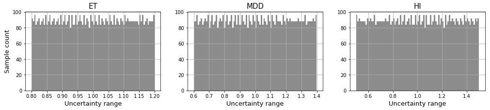
Figure A1 Illustration of the automatically generated samples for the chosen uncertainty variables ET (exposure), MDD (mean damage degree) (impact function) and HI (hazard intensity), with a sample number of N=8000.

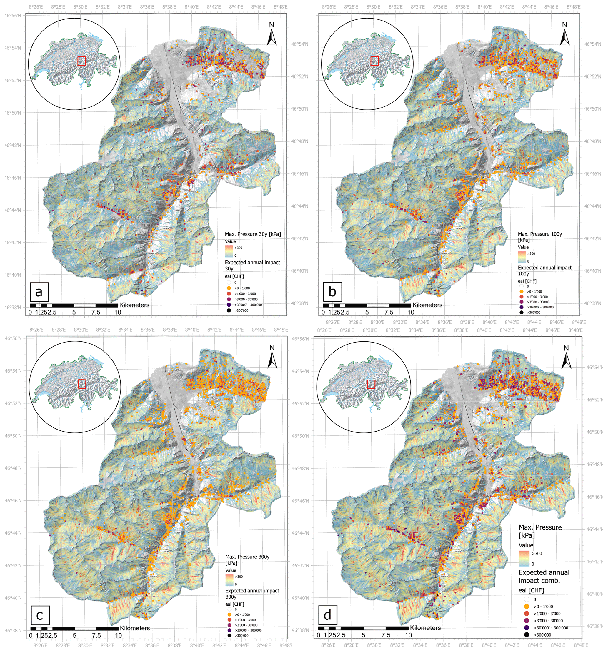
Figure A2 Additional risk maps: overview of the spatial distribution of expected annual impact for individual objects at the three different avalanche scenarios (a) 30 return period, (b) 100 return period and (c) 300 return period and (d) all hazard scenarios combined. Basemap origin (a–d) Swiss federal office of topography: Swisstopo.