the Creative Commons Attribution 4.0 License.
the Creative Commons Attribution 4.0 License.
 | 07 Jun 2023
The influence of large woody debris on post-wildfire debris flow sediment storage
Luke A. McGuire
Katherine R. Barnhart
Ann M. Youberg
Daniel Cadol
Alexander N. Gorr
Olivia J. Hoch
Rebecca Beers
Jason W. Kean
Debris flows transport large quantities of water and granular material, such as sediment and wood, and this mixture can have devastating effects on life and infrastructure. The proportion of large woody debris (LWD) incorporated into debris flows can be enhanced in forested areas recently burned by wildfire because wood recruitment into channels accelerates in burned forests. In this study, using four small watersheds in the Gila National Forest, New Mexico, which burned in the 2020 Tadpole Fire, we explored new approaches to estimate debris flow velocity based on LWD characteristics and the role of LWD in debris flow volume retention. To understand debris flow volume model predictions, we examined two models for debris flow volume estimation: (1) the current volume prediction model used in US Geological Survey debris flow hazard assessments and (2) a regional model developed to predict the sediment yield associated with debris-laden flows. We found that the regional model better matched the magnitude of the observed sediment at the terminal fan, indicating the utility of regionally calibrated parameters for debris flow volume prediction. However, large wood created sediment storage upstream from the terminal fan, and this volume was of the same magnitude as the total debris flow volume stored at the terminal fans. Using field and lidar data we found that sediment retention by LWD is largely controlled by channel reach slope and a ratio of LWD length to channel width between 0.25 and 1. Finally, we demonstrated a method for estimating debris flow velocity based on estimates of the critical velocity required to break wood, which can be used in future field studies to estimate minimum debris flow velocity values.
- Article
(9872 KB) - Full-text XML
- BibTeX
- EndNote


It has long been recognized that large wood influences a variety of hydraulic, ecologic, and sediment transport processes in fluvial systems (e.g., Swanson and Lienkaemper, 1978; Abbe and Montgomery, 1996; Montgomery et al., 2003a; Wohl, 2013). For example, large woody debris (LWD) (>10 cm diameter and >1 m length; Comiti et al., 2016) creates habitat complexity and functionality for ecological processes in flowing streams (e.g., Montgomery et al., 2003b; Vaz et al., 2013). In addition, channel reaches with LWD tend to retain sediment for longer periods of time (Faustini and Jones, 2003; Grabowski and Wohl, 2021) because LWD increases the sediment storage capacity (e.g., Keller and Swanson, 1979; Megahan, 1982; Montgomery et al., 1996; May and Gresswell, 2003) and dissipates energy, encouraging deposition (Richmond and Fauseh, 1995). Wood can be introduced into channels by mass movement such as landslides, streambank failure, and debris flows (Swanson and Lienkaemper, 1978; Montgomery et al., 2003b; May and Gresswell, 2003; Wohl et al., 2009; Chen et al., 2013; Lucía et al., 2015; Surian et al., 2016). Moreover, processes such as root weakening, wind throw, and disease are enhanced in forests burned by wildfire, which accelerates the introduction of wood into channels (Benda et al., 2003; Zelt and Wohl, 2004; Chen et al., 2005; Jones and Daniels, 2008; Bendix and Cowell, 2010).
The interaction between debris flows and LWD is complex because debris flows both scour (e.g., May and Gresswell, 2003; Vascik et al., 2021) and deposit LWD (e.g., Montgomery et al., 2003b; May and Gresswell, 2004) in channels. LWD scoured by debris flows can remain entrained for the full runout zone of a debris flow (Booth et al., 2020). In cases where large amounts of LWD are moving within a debris flow, the runout length tends to be shorter than in debris flows with less LWD (Booth et al., 2020; May and Gresswell, 2004). Shorter runout distances have been attributed to the jamming effects of wood (Booth et al., 2020), and modeling has shown that large wood entrained in debris flows can reduce the flow velocity, which could further reduce the runout distance (Lancaster et al., 2003). In some debris flows, LWD can be deposited at various points along the runout path. Changes in the local geomorphology (e.g., slope change at tributary junctions or channel width) can encourage LWD deposition, and LWD can also be stopped by in-channel immobile objects (e.g., standing trees, large boulders), creating barriers that retain upstream sediment (Montgomery et al., 2003b; May and Gresswell, 2004; Lancaster and Grant, 2006).
From a hazard perspective, the incorporation of LWD in debris flows poses a threat to human life and infrastructure (e.g., Comiti et al., 2016). Damage to roads, bridges, and reservoirs from large wood transport has been documented during flood events (Shrestha et al., 2012; Lucía et al., 2015; Surian et al., 2016; Steeb et al., 2017; Piton et al., 2020), and the majority of wood supplied to the floods originated from landslides and debris flows in low-order drainages or on hillslopes (Chen et al., 2013; Lucía et al., 2015; Surian et al., 2016; Comiti et al., 2016; Rathburn et al., 2017). LWD has also been shown to support sediment retention in landslide dams (Struble et al., 2021). These large wood debris jams can break catastrophically (Swanson and Lienkaemper, 1978; Coho and Burges, 1994; Abbe and Montgomery, 2003), sending a destructive wave of debris and water downstream. The depth of flow moving downstream is amplified above water-only flow by the sediment and debris, making these flows more destructive (Kean et al., 2016).
In this study, we examined the role of LWD in sediment storage of debris flow deposits. Understanding and predicting the volume of debris flow deposition in a watershed are important for hazard assessment. Studies have used debris flow or debris-laden flood observations to develop predictive models of sediment transported after wildfires (Gartner et al., 2014; Pelletier and Orem, 2014; Nyman et al., 2015; Rengers et al., 2021). Although these models implicitly include any sediment retention by LWD, the current predictive approaches do not explicitly account for the sediment storage potential created when wood self-organizes in a channel to block the upstream debris flow sediment. Therefore, we explored the ability of LWD to store debris flow sediment after several runoff-generated debris flows following the 2020 Tadpole Fire in the Gila National Forest in New Mexico, USA. In this study, we specifically investigated how LWD characteristics (e.g., diameter, length, class) influenced the deposit volume that was retained. In addition, we explored relations between the deposit volume retained by LWD and the local geomorphic characteristics (e.g., channel slope, channel width, drainage area). Through this work we are able to better understand and anticipate how LWD may control debris flow sedimentation, and we established a new approach for estimating the critical velocity required to break wood in order to back calculate debris flow velocity in forested settings. Understanding the flow velocity helps to constrain model estimates of debris flow runout (Barnhart et al., 2021) and building damage (Kean et al., 2019).
The Tadpole wildfire started on 6 June 2020 in the Gila National Forest and burned 45 km2 before containment in July 2020. The pre-fire vegetation was dominated by ponderosa pine (Pinus ponderosa). The local geology is composed of tertiary-aged rhyolitic volcanic rocks, pyroclastic rocks, and ash flow tuffs of the datil group (Scholle, 2003). The dominant soils on the site are Mollisols, Inceptisols, and Alfisols (U.S. Forest Service, 2020), and the grain size suggests a loam texture (43 % sand, 45 % silt, 12 % clay). This study focused on debris flows that initiated near the crest of Tadpole Ridge in four watersheds burned primarily at moderate-to-high severity (Fig. 1 and Table 1). The study area falls within a semi-arid climate with annual rainfall totals from 40 to 100 cm, and rainfall occurs primarily during the summertime as part of the North American monsoon (Bonnin et al., 2006).
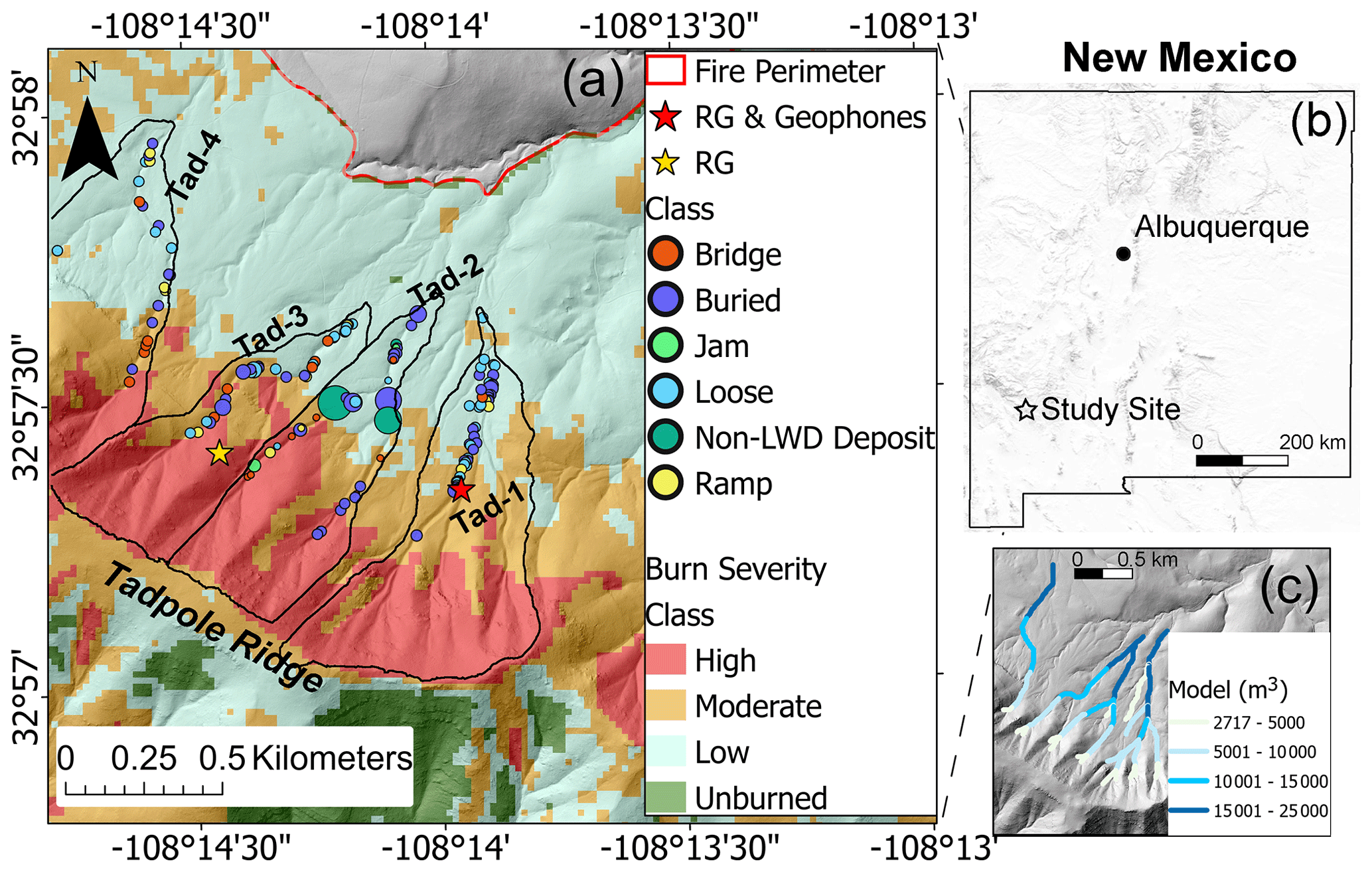
Figure 1(a) Study area within the Tadpole wildfire perimeter. LWD and/or debris flow deposit measurement locations within four watersheds (Tad 1 to Tad 4) are identified. The size of the dots on the map scales between the minimum (0 m3) and maximum volume (208 m3) observed at each LWD and/or debris flow measurement location. (b) Location of the study site within the state of New Mexico, USA, with shaded relief showing topography within the state. (c) Gartner et al. (2014) model predictions of debris flow volume using the maximum rainfall intensity observed at the geophone location. Note that the extent of panel (c) is approximately the same as panel (a).
Table 1Watershed characteristics. The deposit volumes for each watershed are shown as either trapped by LWD or unconstrained (i.e., the deposit stops without any interference by LWD). Note that burn severity for each watershed is labeled as low, moderate (mod), and high. Watershed locations are displayed in Fig. 1.
n/a: not applicable.
At this study site, abundant woody debris was available on the forest floor after the wildfire, as well as trees that remained upright after burning. The large diameter of ponderosa pine woody debris is unlikely to be fully consumed during short-duration fires, as the consumption of wood is related to wood diameter. For example, round-diameter deadwood 1 h fuels are ≤0.64 cm, 10 h fuels are 0.64–2.5 cm, and 100 h fuels are 2.5–7.6 cm (National Wildfire Coordinating Group, 2022). Because wildfire duration is typically less than 10–100 h, we expect large-diameter wood (e.g., >10 cm) to remain in the forest and to be available to interact with channel sediment after wildfires. Moreover, ponderosa pine wood diameters >10 cm differentiate this site from locations such as the San Gabriel Mountains in California, the location of many post-fire debris flow observations (e.g., Cannon et al., 2008; Kean et al., 2011; Tang et al., 2019; Palucis et al., 2021). The San Gabriel Mountains are primarily vegetated by chaparral plants, which are sclerophyllous woody shrubs found in semi-arid environments that are prone to burn every 30–150 years (Halsey, 2005). The maximum diameter of chaparral plant stems falls between the 1 and 10 h fuel diameters (Conard and Regelbrugge, 1994), and chaparral stems are frequently fully consumed during wildfires.
The following subsections outline the methods used in this study, including in situ field instrumentation, airborne lidar, and field mapping. We also describe the analytical methods used to compare volume measurements with existing empirical volume models. Finally, we outline a new method for using wood observations to estimate flow velocity.
3.1 Instrumentation, mapping, and measurements
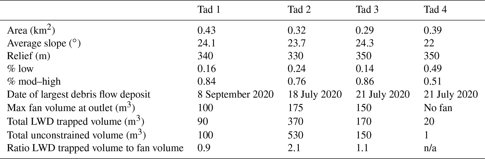
We installed equipment to monitor runoff and debris flow responses from four watersheds on 6–7 July 2020, while portions of the Tadpole wildfire were still burning (Tad 1, Tad 2, Tad 3, and Tad 4; Fig. 1). Monitoring equipment for this study was clustered at two locations: one location included a stand-alone rain gauge (RG), and the second location included a rain gauge with paired geophones to record the timing and velocity of debris flows (RG and geophones) (Fig. 1). The geophones (single component, Geospace GS11) were emplaced into the ground using a spike that contacted the soil. They were programmed to only turn on during rainfall, and they recorded at a rate of 50 Hz. At the geophone location, the geophones were aligned on the channel bank parallel to the channel (Fig. 2). The geophones were located a horizontal distance of 13.9 m from the channel edge, a vertical distance of 3.1 m above the channel thalweg, and they were spaced 14.6 m apart (Fig. 2).
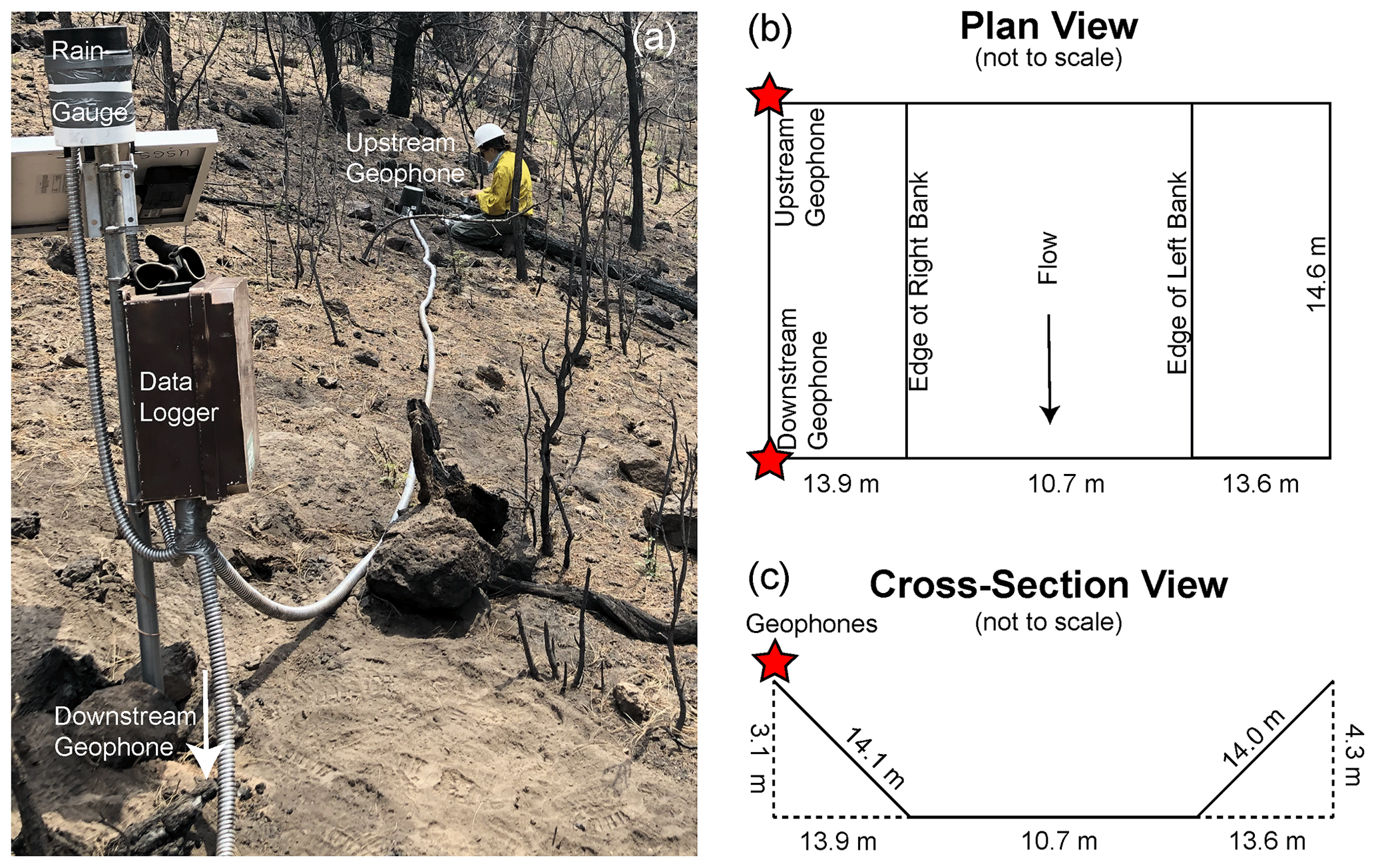
Figure 2Schematic showing the geophone setup. (a) Photo of the rainfall-triggered geophone setup. Note that the downstream geophone location is out of view. Photo credit: Francis K. Rengers. (b) Plan view dimensions of the channel, channel banks, and geophones. (c) Cross-sectional view of channel and geophone location.
In the watershed monitored using geophones, we estimated the debris flow velocity by using a cross-correlation analysis to estimate the time difference between the absolute value of the two geophone measurements (mV) similar to Kean et al. (2015) (data available in Rengers et al., 2022b). Additionally, we filtered the signal using a 5 s median filter and divided each geophone signal (mV) by the maximum value during the storm. Using this instrumentation, in addition to field visits, we were able to identify post-wildfire rainstorms that resulted in runoff-generated debris flows.
We mapped debris flow deposits in four watersheds using ArcGIS Collector (Fig. 1). The volume of each debris flow deposit was estimated as a sediment wedge using a measuring tape, similar to the approach described by Lancaster et al. (2003). Photographs were obtained at each deposit location and attached to the collector points (data available in Rengers et al., 2022a).
In the same four watersheds, we also mapped the LWD in channels. LWD was classified using terminology borrowed from the fluvial literature to describe mapped wood as buried, loose, ramp, bridge, or jam (Fig. 3) (Kramer and Wohl, 2017). Buried LWD is defined here as wood that is contained within and underneath sediment. Buried LWD can also be pinned by a tree, boulders, or other wood in a wood jam. When wood is pinned, debris flow sediment pushes the wood against a large object with enough resistance to keep the wood in place. In these cases the buried wood can help to retain sediment within a channel such that, without the buried/pinned wood, it is unlikely that sediment would have deposited at that specific location in the channel (Fig. 3). By contrast, loose LWD is stratigraphically on top of a sediment deposit or the channel. Loose pieces can float during water flows or become pinned by downstream trees, boulders, or jams, but they do not actively retain any sediment. Bridge LWD are wood pieces that are longer than the channel width and therefore span the channel banks, often not interacting with the channel flow or sediment. Ramps are loose LWD that have fallen into the channel, and a portion of the LWD remains on the channel bank. Ramps can be pinned by downstream obstacles or partially buried to retain sediment in the flow, but they protrude out of the active channel. Finally, jams are composed of many pieces of LWD interlocked via friction that block a portion of the channel.
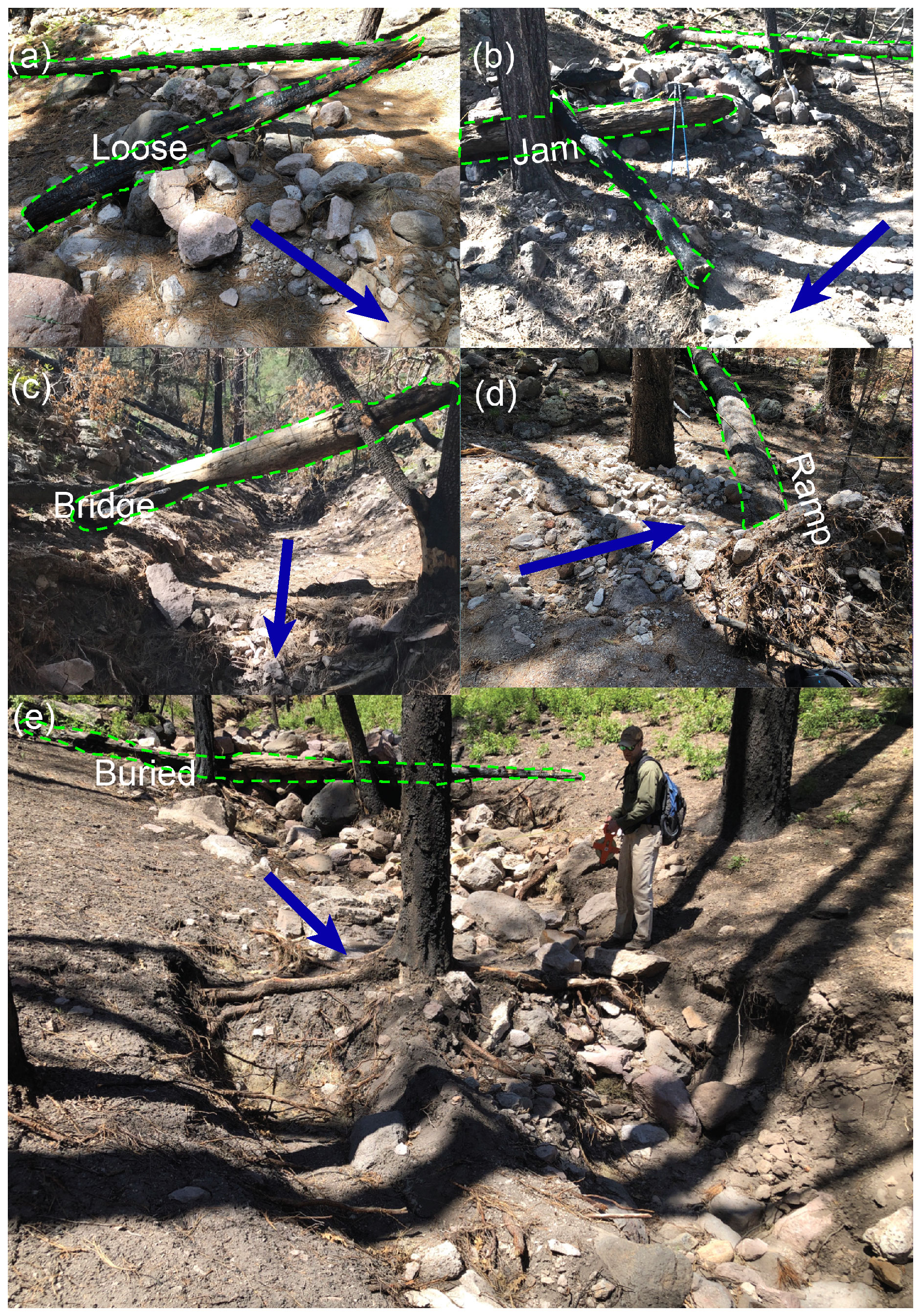
Figure 3Photographs showing each LWD class. Dashed lines help to identify the wood pieces, and arrows indicate the direction of flow. Photo credit: Francis K. Rengers.
We used pre-event high-resolution topographic data to explore the connection between the geomorphology of the debris-flow-producing watersheds and the deposits forced by LWD. Airborne lidar data were flown prior to the fire on 27–28 March 2019 with a ground point density of 4.9 points m−2. We obtained the lidar point clouds from the National Map (U.S. Geological Survey, 2019) and stitched them together using LAStools (rapidlasso GmbH, 2022) in order to create a hydrologically connected digital elevation model (DEM). We used this pre-fire lidar data from the study site to compare the length of the LWD to the pre-debris flow channel width, and we examined the relationship between pre-event slope and deposit volume.
In order to extract the channel width, we first defined the stream channels using the hydrologic toolset in ArcGIS Pro 2.8.3, calculating the upstream contributing drainage area using a D8 flow-direction algorithm. This flow accumulation grid was subsequently used to identify the stream network with a threshold contributing area of 0.01 km2. We then created stream cross-sections perpendicular to the stream channels at a spacing of 5 m, and we associated each debris flow deposit with the nearest cross-section. For each cross-section near a measured deposit, we extracted the x, y, z values from the DEM underlying each cross-section. Using the cross-sectional profile (Fig. 4a), we defined the active channel width as the flow width 1 m above the lowest elevation in the channel, which corresponded to the peak flow depth observed in most channels during field observations. Topographic measurements of the active channel width derived from lidar were compared against field measurements of the active channel width.
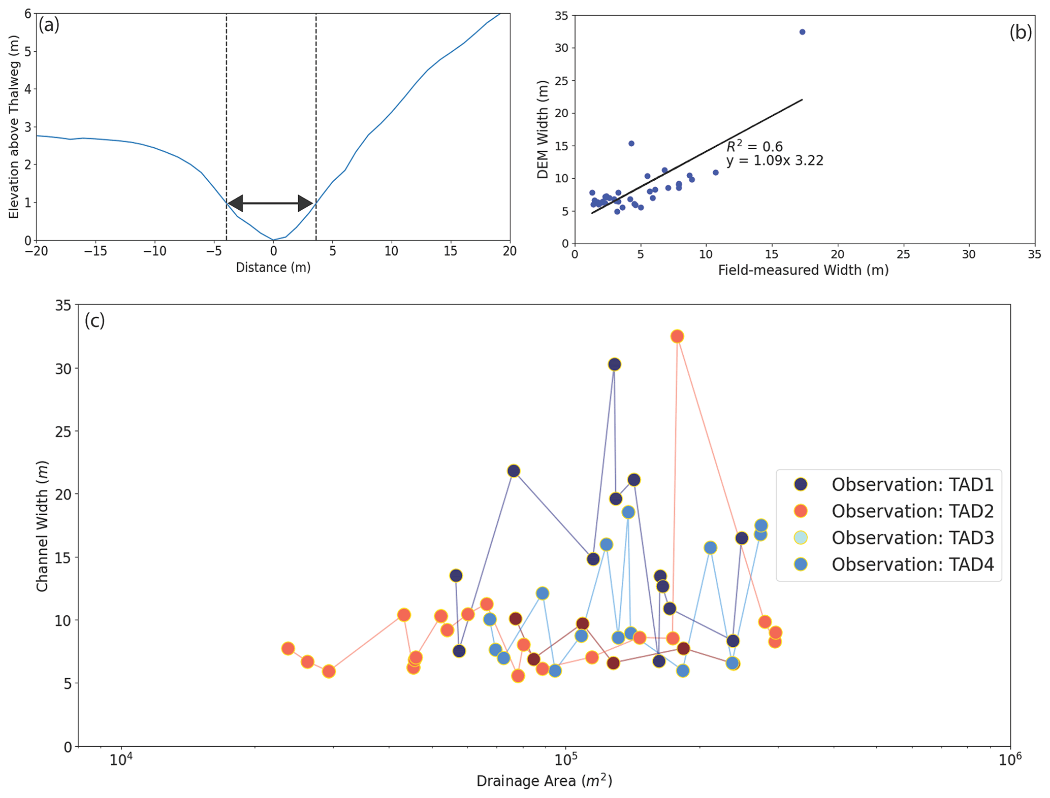
Figure 4Analysis of channel width extracted from the pre-event digital elevation model and field measurements. (a) Blue line shows one of the cross-sections extracted from the lidar DEM. The cross-section has been centered so that the thalweg is located at 0 m, and the distance away from the thalweg is shown as either positive or negative values. Dashed lines were automatically determined at the location on each bank that is 1 m above the thalweg. Arrows indicate the channel width measurement location. (b) Plot of field measurements of channel width versus measurements obtained automatically from the lidar data. (c) Channel width with respect to drainage area; note semi-log axes.
Prior work has recognized that LWD deposition in a channel is related to the length of the LWD (L) versus the channel width (W) (Vaz et al., 2013). Herein we define this ratio as
We examined the volume of debris flow sediment stored behind LWD with respect to ζLW. In addition, buried, jam, and ramp LWD classes were influential in storing sediment when they were pinned against an object such as a tree or large rock that did not move in the flow. Therefore, we accounted for whether LWD was pinned at a location of sediment deposition. In this analysis we eliminated all LWD measurement locations where no sediment was stored (volume =0 m3). This eliminated all of the bridges and loose LWD from the analysis because neither led to the storage of sediment.
3.2 Volume models
The debris flow deposit volumes in our study area were further compared to modeled predictions of debris flow volume. The US Geological Survey (USGS) debris flow hazard assessment uses a model developed by Gartner et al. (2014) in the Transverse Range of southern California to estimate debris flow volumes. The volume model has the following form:
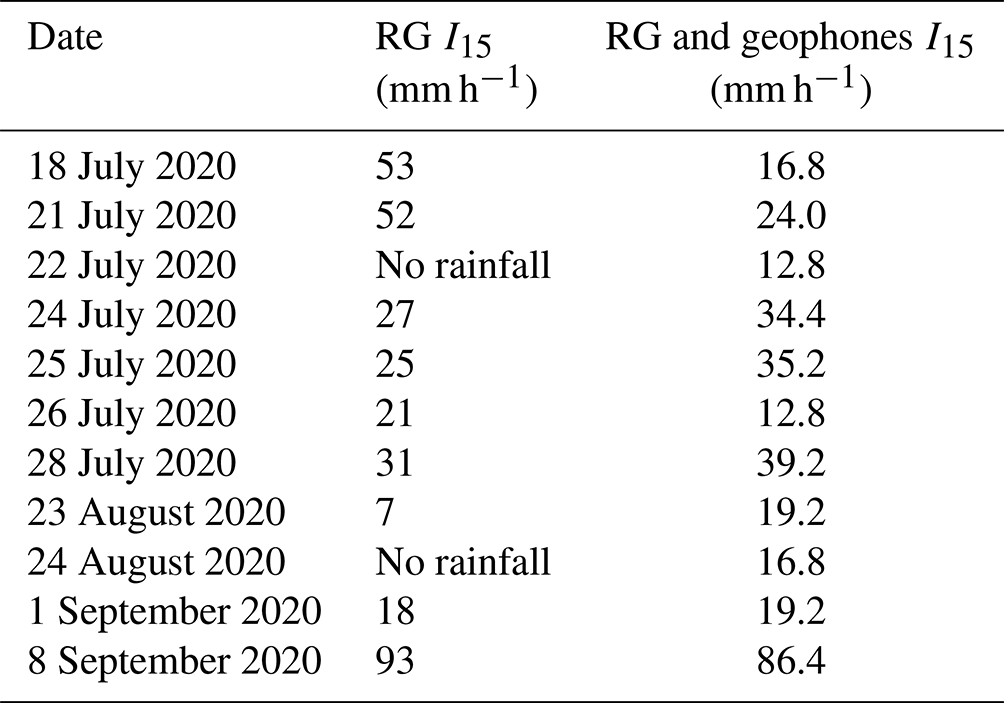
where V is volume (m3), I15 is the 15 min rainfall intensity (mm h−1), Bmh is the watershed area burned at moderate and high severity (km2), and R is the watershed relief (m). The model was developed in an area dominated by chaparral shrub forests and scrub oak vegetation at elevations below 1520 m a.s.l. and conifer forests above 1520 m a.s.l. with Douglas-fir (Pseudotsuga macrocarpa), coast Douglas-fir (Pseudotsuga menziesii var. menziesii), ponderosa pine (Pinus ponderosa), white fir (Abies concolor), and lodgepole pine (Pinus contorta) (U.S. Forest Service, 2022). Because of the large swaths of chaparral, the availability of large wood able to retain debris flow sediment is reduced compared to forests with larger trees, such as the Tadpole study site. This model is applied to channel segments modeled as part of a USGS debris flow hazard assessment (U.S. Geological Survey, 2022), and values for ln (Bmh) and are calculated for each segment. For the rainfall intensity parameter in Eq. (2), we used the gauge labeled RG & Geophones (Fig. 1) for drainages Tad 1 and Tad 2 and the gauge labeled RG (Fig. 1) for drainages Tad 3 and Tad 4. For this calculation, we used the maximum observed I15 at each of the rain gauges for the highest-intensity rainstorm on 8 September (Table 2). This was not the only debris-flow-producing storm, but it was the storm with the highest intensity, and therefore the calculated volumes would show maximum potential volume.
In addition to the Gartner et al. (2014) model, we used a model developed in New Mexico to predict sediment yield associated with debris-laden flows to compare with our observations (Pelletier and Orem, 2014):
where Yp is sediment yield in mm, S is average basin slope (m m−1), B is average soil burn severity, a=1.53, b=1.6, and c=1.7. The categorical burn severity variables are converted to the following unitless values: low =1, moderate =2, and high =3. The coefficients used in Eq. (3) could be calibrated to any regional setting; however, because this study site is near the area where the model was developed, we used the original coefficients. The sediment yield Yp was converted from units of millimeters to meters and multiplied by the upstream basin area in order to obtain a volume. This model was developed following debris flows that initiated in an area with large trees and deposited sediment in a fan dominated by grass and shrubs (Pelletier and Orem, 2014). Pelletier and Orem (2014) describe the vegetation of their study area as ponderosa pine and Gambel oak (Quercus gambelii) below 2740 m a.s.l., Douglas-fir (Pseudotsuga menziesii), white fir (Abies concolor), blue spruce (Picea pungens), and aspen (Populus tremuloides) between 2740 and 3040 m a.s.l., and Engelmann spruce (Picea engelmannii) and corkbark fir (Abies lasiocarpa var. arizonica) >3040 m a.s.l.
The volume models are expected to predict the total volume passing a location, whereas the total volume retained behind LWD only reflects the amount of material that was stopped by LWD. Consequently, we compared the maximum modeled volume with the volume of terminal fans in Tad 1–3. Tad 4 did not have a terminal fan at the basin outlet, so the nearest deposit behind LWD was used. For additional context, we compared the total volume stored behind LWD upstream from the terminal fan with the fan deposits and modeled fan volumes.
3.3 Velocity estimates from wood measurements
Understanding breaking forces/velocities may help to identify the threshold where LWD substantially influences exported sediment volumes. Therefore, we related wood size to breaking velocity, which is the velocity of flow required to break wood, assuming greenstick fracture behavior as the failure mechanism for both unburned and partially burned wood (Ennos and Van Casteren, 2010). Wood transported in a debris flow experiences large forces that may splinter or break the wood into smaller fragments. The size of the wood remaining after a debris flow event may provide constraints on the debris flow velocity in that velocities in excess of an estimated breaking velocity were likely not experienced. The estimated breaking velocity should thus be considered the flow velocity threshold necessary to break LWD. To estimate the breaking velocity, we consider the wood a cylindrical beam with length L and diameter D that is pinned either by two downstream trees – one at each end – or by one downstream tree located at the midpoint, . The beam is subjected to a uniform force per unit length f directed in the downstream direction. This uniform force bends the LWD, imparting a maximum bending moment M, in both idealized geometries, occurring at the mid-point of the LWD piece.
A complete description of f would necessitate describing the depth-variable flow field of the debris flow front, including the force of impact imparted by entrained boulders. As a rough approximation, we considered only the force imparted by fluid drag. We assumed that the LWD piece was fully submerged and that flow was both above and below the tree in order to calculate the total drag force F as (e.g., Abbe and Montgomery, 1996; Manners et al., 2007)
where u is the downstream velocity, ρ is the fluid density, Cd is the drag coefficient, and A is the cross-sectional area facing the flow (). We used a weighted average density of ρ=1680 kg m−3, reflecting a solid volume fraction of 0.6, a sediment density of 2700 kg m−3, and a fluid density of 1000 kg m−3. We used a value for Cd=1.17 corresponding to a submerged cylinder. The force per unit length is given as
As discussed by Ennos and Van Casteren (2010), LWD pieces and other natural beams are stronger in the longitudinal direction (parallel to L) and typically break in the transverse direction. Accordingly, we assumed that failure always occurred in the transverse direction. We used Eq. (2.8) from Ennos and Van Casteren (2010) to calculate the maximum transverse stress, σT, within the LWD piece as a function of D and M.
We assumed that LWD broke when the maximum transverse stress was equal to the yield strength, equivalent to a factor of safety of 1. We calculated the value of u at yield by combining Eqs. (4), (6), and (7) and rearranging for u:
where σTy is the transverse yield strength, calculated using Eq. (3.3) from Ennos and Van Casteren (2010), which incorporates an assumed tree density of 500 kg m−3 (Engineering Toolbox, 2022). Equation (8) implies that for a constant ratio of the breaking velocity is constant. We then used field measurements of D and L to calculate u at locations where LWD was pinned against trees.
There were 11 substantial rain events during the summer monsoon period following the wildfire (Table 2). These resulted in multiple runoff-generated debris flows in each basin, and in all of the basins it was possible to identify the date of the largest debris flow (Table 1). Field observations indicated that LWD storage of debris flow material occurred during all of these storms, and thus the measurements represent an aggregate across debris flow events. Note that a terminal deposit in Tad 4 was eroded prior to measurement. The largest recorded storm occurred on 8 September 2020 (Table 2), and the geophones during that storm provided the clearest estimate of debris flow velocity (Fig. 5). Using the data from this storm, we found the maximum lag between the upstream and downstream geophone peaks was 3.6 s, indicating a debris flow velocity of 4.1 m s−1 (Fig. 5).
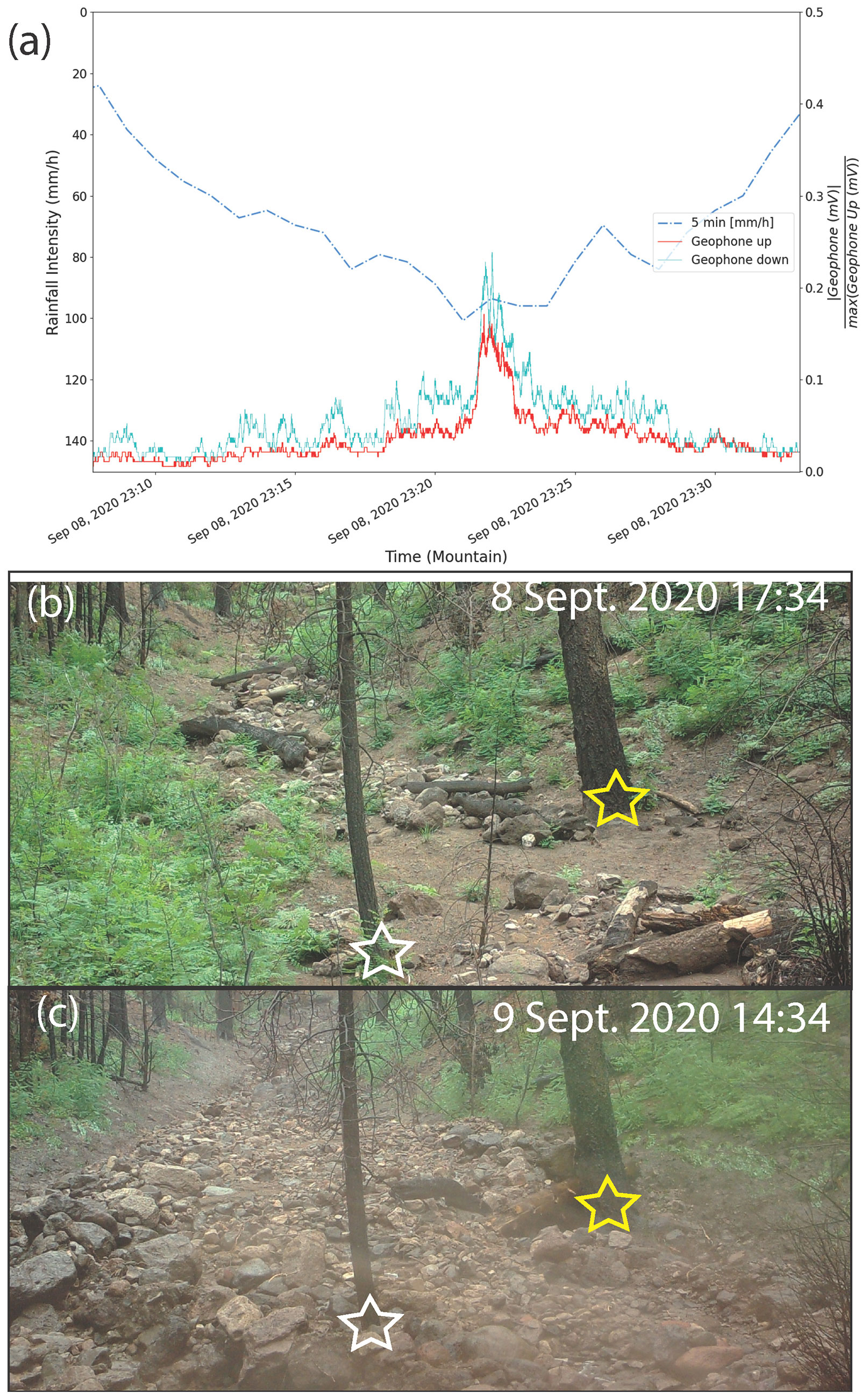
Figure 5(a) Rainfall intensity and corresponding geophone response during a debris flow. “Geophone up” represents the upstream geophone, and “geophone down” represents the downstream geophone. (b) Photo of the channel reach near the geophones on 8 September 2020 at 17:34 local time (LT). Photo credit: Luke A. McGuire. (c) Photo of the channel reach near the geophones following the debris flow on 9 September 2020 at 14:34 LT. Stars indicate the same location in each photo. Photo credit: Luke A. McGuire.
We mapped 218 locations of LWD within the four study watersheds, which were associated with 125 unique debris flow deposits (some deposits had more than one piece of LWD) (Fig. 1). The total volume stored by each LWD class shows that the buried and jam LWD classes were associated with the largest cumulative deposit volume stored (Fig. 6). Buried and jam LWD at the field site were often pinned against stable objects such as standing trees or boulders, and the buried wood pieces created a barrier that retained an upstream sediment deposit (Fig. 6). Loose wood was also found in debris flow deposits, possibly deposited during the waning watery tail of debris flows, but loose wood did not provide any structural stability that would retain the deposit (Figs. 3 and 6). Finally, ramps were associated with the smallest deposit volumes (Fig. 6).
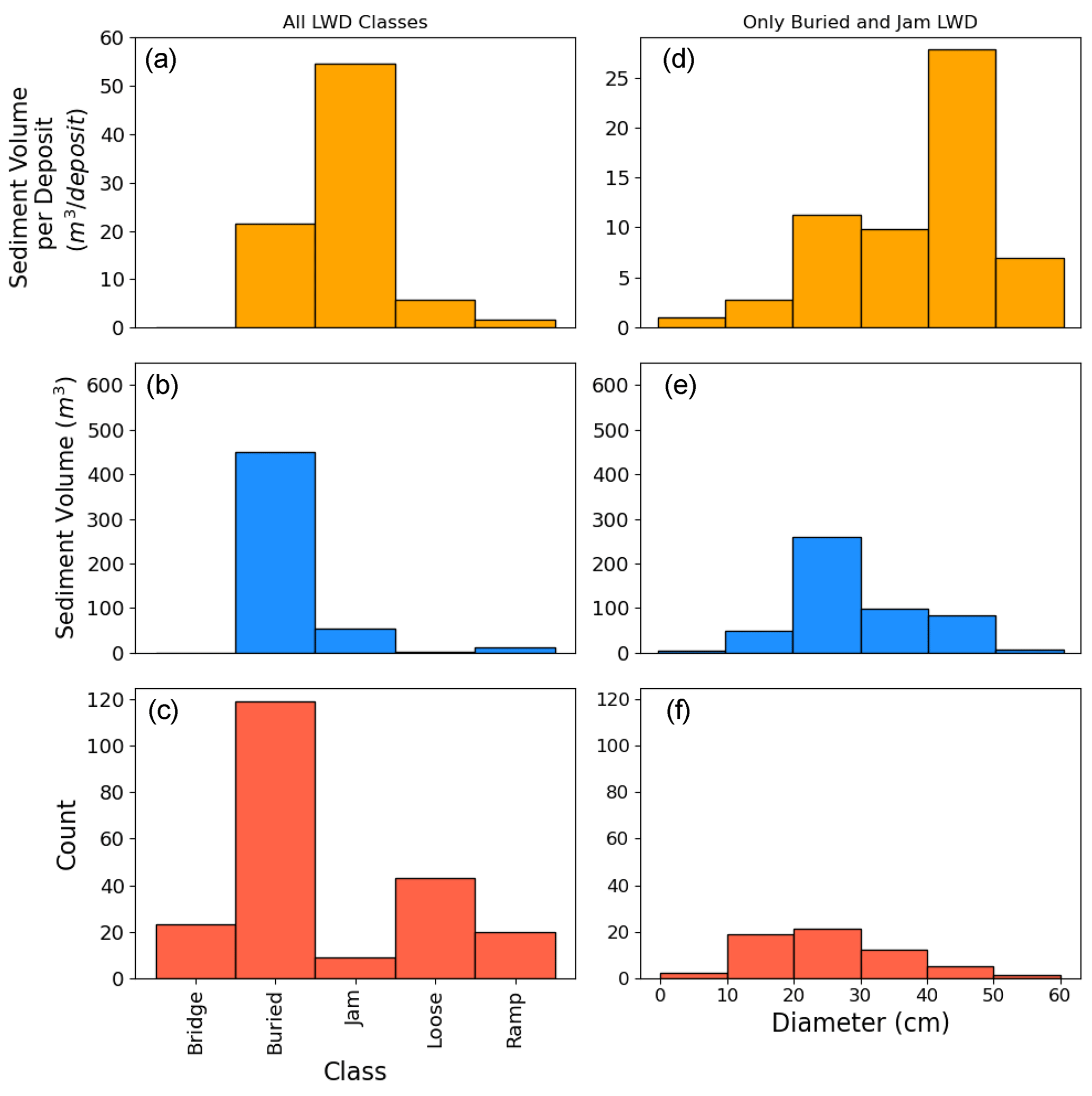
Figure 6(a) The total volume of trapped sediment divided by the total number of deposits within each LWD class. (b) The total volume of trapped sediment measured within each LWD class. (c) Histogram showing the number (total count) of LWD pieces within each LWD class. (d) The total volume of trapped sediment behind either buried or jam LWD classes divided by the total number deposits within LWD maximum diameter classes. (e) The total volume of trapped sediment behind either buried LWD or jam LWD classes. (f) Histogram showing the number (total count) of the maximum LWD diameter at each deposit. Note for both panels (a) and (b) if there were multiple LWD pieces of different classes at a deposit (e.g., buried and loose), the class that functionally retains sediment (e.g., buried) was used. For panels (d)–(f), the diameter is the maximum LWD diameter measured at each deposit and binned in 10 cm intervals.
We compared the maximum measured LWD diameter of buried and jam LWD classes to the deposit volume (Fig. 6d–f), limiting our analysis to these two classes because they were associated with the largest deposits. LWD with diameters larger than 20 cm were associated with larger sediment deposits. Additionally, as the LWD diameter for these two classes increases, the number of observations decreases, but the total stored volume per number of deposits increases (Fig. 6d). For example, 50 % of the observed sediment volume was retained behind LWD with a maximum diameter between 20 and 30 cm, but only 30 % of the maximum measured diameters are between 20 and 30 cm (Fig. 6d). Similarly, 16 % of the observed volume was stored behind a maximum LWD diameter of 40–50 cm, but those maximum diameter sizes only represented 8 % of the total measured diameters (Fig. 6d–f).
The ratio of LWD length to channel width (ζLW) also influenced the volume of trapped debris flow sediment. The maximum debris flow deposit volumes were concentrated within a narrow range of (Fig. 7). In the majority of the measurements, LWD was pinned by a larger immobile downstream object, causing sediment to back up behind the LWD. Among the different LWD classes, ramps did not stop a large amount of sediment (Fig. 3), but they span a large range from ζLW less than 1 to ζLW greater than 1. Because many ramps were buried, the true LWD length was likely underestimated in those cases, thus contributing to estimates of ζLW<1. The peak in sediment retention in the range of reflects situations where the wood is small enough to fit in the channel, unlike a bridge, but large enough to take up a large proportion of the channel width where the wood could be wedged between standing trees or boulders within the channel to stop upstream sediment. Buried LWD and jams were the primary classes of LWD associated with ratios between 0.25 and 1, containing the majority of larger deposit volumes (e.g., >10 m3).
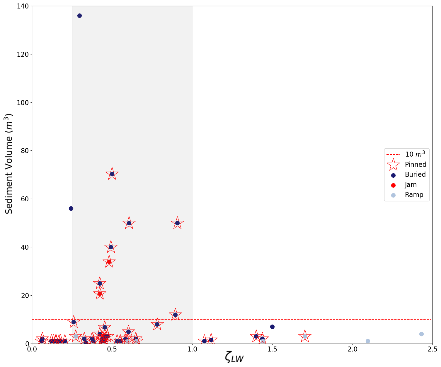
Figure 7A comparison of the ratio of the LWD length to channel width (ζLW) at 1 m above the channel bottom versus the trapped debris flow sediment volume. The color of each point is based on the class of the LWD. The bridge and loose LWD classes were removed because those classes did not actively restrict sediment movement downstream. The shaded gray region denotes the ratio of ζLW values associated with the maximum sediment retention volumes. The dashed line separates deposits greater than and less than 10 m3.
The analysis of sediment volume with respect to channel slope showed no strong relationship between measured volume and slope if all of the measured deposits were considered. However, lower channel slope is correlated with sediment volume above a threshold size of 10 m3 (Fig. 8). The largest debris flow deposits were observed where the local pre-fire channel slope was >5 and <25∘. No post-fire slope data are available in cases where the channel slope may have changed, but qualitative field observations indicate that source areas scoured to bedrock, and steepened and depositional areas aggraded, creating shallower slopes.
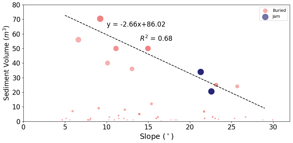
Figure 8Slope angle (degrees) versus the trapped debris flow sediment volume. The points are scaled by deposit volume size between the minimum (12 m3) and maximum (70 m3) volumes in the buried and jam LWD classes. A linear regression line is fit to all deposits larger than 10 m3.
The total volume stored behind LWD was larger or comparable in size to sediment stored in terminal fans for most of the drainages (Fig. 9). The Gartner et al. (2014) volume model overpredicted the volume of the observed terminal fans by 1–4 orders of magnitude, whereas the Pelletier and Orem (2014) model provided estimates that were closer in magnitude to the terminal fan observations (excluding Tad 4 where the terminal fan was removed by erosion).
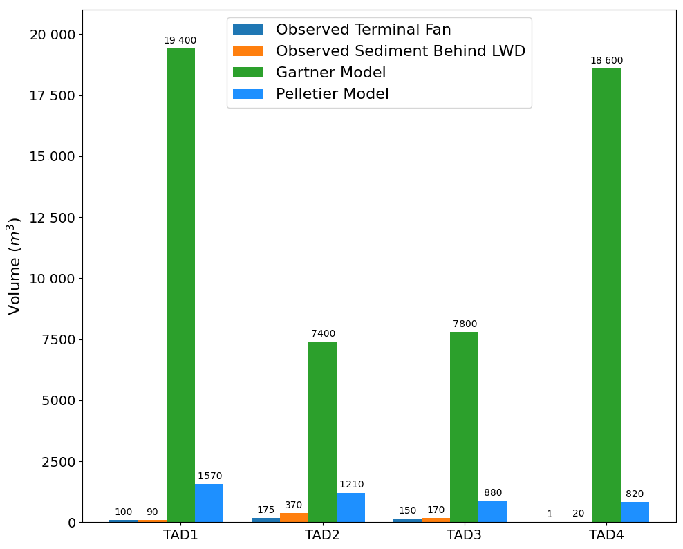
Figure 9Comparison of the trapped debris flow sediment volume behind LWD and the unconstrained debris flow sediment volume stored in terminal fans at the basin outlet. In addition, model estimates of post-wildfire sediment volumes at the basin outlet from Pelletier and Orem (2014) and Gartner et al. (2014) are displayed. The observed and modeled sediment volumes are shown above each bar with units of m3.
Our wood-break analysis showed that the velocity required to break wood (in the considered idealized geometry) varied across wood lengths and diameters. We found clear spatial patterns of velocity by applying the peak velocity from the largest rainstorm on the study site with LWD that was either buried or in a jam. In Tad 1, where the field velocity measurement was made, we found that the measured LWD in the channel are all larger than the wood geometry that would be broken by a velocity of 4 m s−1, with the exception of the LWD at the bottom of the watershed where the channel widens and debris flow sediment is deposited in a fan (Fig. 10). This result agrees well with the breaking velocity approach. In the other drainages (Tad 2–4) wood with measurements below the breaking velocity was primarily located in wide channel reaches where velocity would be expected to slow; otherwise the wood geometry is consistently larger than the modeled breaking velocity (Fig. 10).
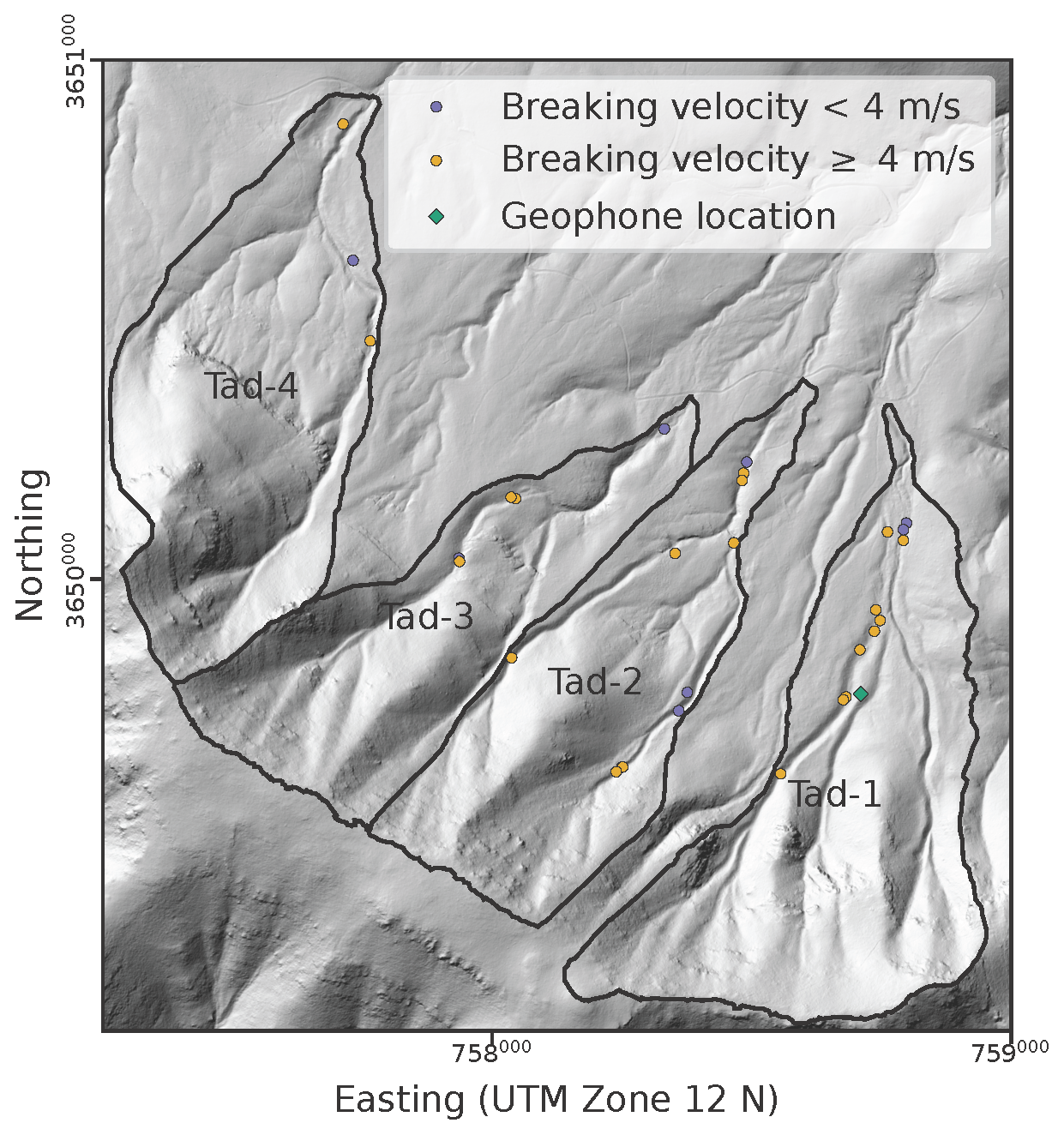
Figure 10Map of estimated velocity based on the wood dimensions. The velocity (4 m s−1) is used as a threshold because it was the maximum velocity measured by the geophones.
This study examines how post-fire debris flows moving through small headwater channels in forested environments retain debris flow sediment, where debris flow sediment is stored, and the geomorphic/wood characteristics that influence local deposition. Field data combined with modeling are used to understand how LWD influences debris flow volume storage and how LWD can be used to estimate flow velocity. Better constraints on sediment volume and velocity will ultimately lead to more accurate debris flow runout modeling and damage assessments (Kean et al., 2019; Barnhart et al., 2021).
Field measurement data indicate that wood characteristics played an important role in the depositional volume and location. For example, the maximum diameter of LWD in a channel reach was related to the total deposit volume stored. The majority of wood diameters measured were greater than 10 cm, possibly because wood of smaller diameters was destroyed by the fire. The total duration of the fire at any location is unknown; however, 10–100 h fuels are 2.5–7.6 cm, and it is likely that wood with diameters less than 10 cm was fully consumed. Consequently, in forest environments with smaller-diameter wood (e.g., chaparral), the effect of wood on sediment storage may be limited compared to forests with larger trees. Moreover, the class of the LWD strongly influenced deposit volume storage, with LWD that was buried or in a jam containing the most sediment (Fig. 3). Ramps retained little sediment, likely because they are unstable features.
The combined influence of channel morphology and LWD also influenced debris flow sediment storage. The ratio of wood length to channel width (ζLW) shows that sediment is preferentially stored where LWD spans at least one-quarter of the channel width. When LWD is longer than the channel width, it does not effectively stop sediment because it cannot be oriented fully perpendicular to the flow field. In cases where the LWD is less than one-quarter of the channel width, the flow can move around or reorient the LWD, making the wood less effective for storage (see Fig. 3b for an example of sediment storage in half the channel width and flow movement through the other half of the channel). Identifying critical reaches of potential sediment storage might be done a priori using channel width measurements from high-resolution topography, if a characteristic LWD length could be estimated in a region. Prior work has shown that channel width increases as a function of discharge (e.g., w=cQb) (Leopold et al., 1964). However, in the steep headwater catchments in our study area, width does not appear to change predictably as a function of drainage area (Fig. 4c). Instead, narrow local channel reaches allowed LWD to deposit and then store debris flow sediment moving from upstream. Our comparison of field-measured active channel width to widths extracted from lidar topography shows a high degree of correlation, indicating that lidar-derived width measurements are a viable alternative when field measurements are difficult to obtain (Fig. 4).
The effect of slope on sediment storage also reflects the interaction between the LWD and channel morphology. There is no relation between slope and all measurements of deposit volume. However, a more narrow analysis of the stored deposit volume >10 m3 shows deposit volume increases as channel slope decreases. This indicates that small amounts of sediment can be retained and stored regardless of the channel slope. However, larger deposits accumulated on shallow slopes. Consequently, energy dissipation on shallow slopes may help to encourage more deposition behind LWD than on steep slopes where flow energy is higher, and slope may be a useful predictor of LWD sediment storage.
The volume of deposition at the terminal fan for each basin outlet modeled using Eq. (2) overpredicted the fan deposit by several orders of magnitude. The Gartner et al. (2014) volume model has been shown to be successful in the region where it was developed (the Transverse Range of southern California) and where a large contribution of sediment is derived from hillslope erosion (Rengers et al., 2021), but it overpredicts at this study site. In contrast, Eq. (3) developed by Pelletier and Orem (2014) predicted sediment volumes at the terminal fan that were closer to the observed volumes. This might be because that model was developed in a similar region of New Mexico, with a similar elevation/climate (both at 2500–3000 m) and lithology (rhyolite). The forced storage of debris flow sediment by LWD in the Tadpole study area retained a larger or comparable volume of sediment, as was observed at the terminal fan of the basin outlets, which may explain some deviations from the Pelletier and Orem (2014) volume model. Moreover, the Tadpole study area has steep slopes on Tadpole Ridge that rapidly decrease at drainage areas of less than 1 km2 (Table 1), but the region studied by Pelletier and Orem (2014) maintained steady slopes and channel scour at larger drainage areas prior to deposition (greater than 1 km2). Therefore, the total volume observed in their model may be calibrated on observations of more sediment scour. Consequently, regionally calibrated empirical models may be the best approach for regional volume predictions, but local influences of site geomorphology may add to variability in predictions versus observations.
Our greenstick analysis of wood breakage helps to quantify the flow threshold where LWD may no longer have a substantial effect on retaining sediment. As flows become larger and increase in velocity, LWD will break or move and retain fewer debris flow deposits. The presence of unbroken wood pinned against trees after the debris flow events implies that those wood pieces did not experience stresses in excess of yield strength. Our wood-breaking velocity analysis using Eq. (8) agrees well with field observations. Some of the wood-breaking velocities for selected LWD in relevant geometries are lower than the observed peak velocity at the geophones of 4 m s−1 (Fig. 10). These deviations likely reflect potential for velocity differences across channels Tad 1 to Tad 4, as well as changes in channel morphology that could reduce flow speed, such as wide channels or lower slopes. Despite these uncertainties, overall the predicted velocities generally correspond with our expectations of wood larger than a breaking velocity of 4 m s−1 in the narrow confined channels and less than the breaking velocity at wide channel sections or near the basin outlet where the channel becomes unconfined. Therefore, this approach may be a potential tool for estimating debris flow velocities, which could be used to constrain model simulations.
In summary, this study indicates that in regions where there is a potential for substantial LWD interaction with debris flow sediment, the LWD may strongly control the overall location of sediment deposition and alter predictions of deposit volume. The amount of sediment stored behind LWD exceeded the sediment deposited in the terminal fan in three out of four cases. In situations where the debris flow momentum was smaller than the breakage capacity of the wood, we saw that LWD can substantially influence debris flow sediment storage. However, in larger debris flows, LWD may not be sufficient to retain sediment within the channel before reaching a terminal deposition zone (Booth et al., 2020). Consequently, the effect of LWD on sediment storage will be dependent on the rainfall rate (Gartner et al., 2014), which ultimately controls the debris flow size and watershed characteristics, such as channel width variations. In addition, debris flow sediment stored by LWD may periodically load channels with sediment, potentially leading to more extreme responses and downstream sedimentation during future storms when this sediment is mobilized. At this study site, sediment stored behind wood with diameters exceeding 10 cm may remain in channels and be available for future debris flows because of the slow decay rate for wood with D>10 cm (Harmon and Sexton, 1996). These observations give a snapshot of the influence of LWD for an observed set of rainfall and watershed characteristics. More work would be beneficial to develop a framework to model the potential storage as a function of rainfall intensity, stem density, drainage area, and channel width.
Large woody debris (LWD) is often entrained and transported during debris flows. In some cases the LWD can interact with the flow to retain sediment in channels, which influences predictions of debris flow volume expected at channel outlets. In this study we observed that debris flow sediment retention in steep headwater streams was dependent on both the characteristics of the LWD and the channel morphology. LWD with larger diameters retain more sediment, and the ratio of LWD length to channel width strongly controls sediment retention. The largest deposits were found at the lowest channel slopes; however, LWD retained small volumes of debris flow sediment regardless of the overall channel slope. Future predictions of the location of debris flow sedimentation in small headwater streams could be achieved by estimating a characteristic wood length and identifying areas where the ratio of wood length to channel width is between 0.25 and 1. Additionally, we found that observations of LWD dimensions sufficient to hold back sediment without breaking may be a useful future tool for estimating debris flow velocity, and this may be helpful in determining thresholds below which LWD may influence deposit volumes.
Data used for the analyses in this study are available in Rengers et al. (2022b, https://doi.org/10.5066/P9I564PP) and Rengers et al. (2022a, https://doi.org/10.5066/P9NYZ9JC).
FKR, JWK, LAM, and AMY developed the field instrumentation design. DC designed the field survey strategy. LAM, FKR, AMY, ANG, OJH, KRB, and RB helped with field data collection and collation. KRB led the wood-break velocity analysis. FKR prepared the manuscript and performed the data analysis with contributions from all co-authors.
The contact author has declared that none of the authors has any competing interests.
Any use of trade, firm, or product names is for descriptive purposes only and does not imply endorsement by the US Government.
Publisher’s note: Copernicus Publications remains neutral with regard to jurisdictional claims in published maps and institutional affiliations.
This work was supported in part by the US Geological Survey Landslide Hazards Program. The authors are grateful for helpful review feedback from Jon Pelletier, Helen Dow, and Andrew Mitchell, as well as one anonymous reviewer.
This paper was edited by Olivier Dewitte and reviewed by Andrew Mitchell and one anonymous referee.
Abbe, T. B. and Montgomery, D. R.: Large woody debris jams, channel hydraulics and habitat formation in large rivers, Regul. River., 12, 201–221, https://doi.org/10.1002/(SICI)1099-1646(199603)12:2/3<201::AID-RRR390>3.0.CO;2-A, 1996. a, b
Abbe, T. B. and Montgomery, D. R.: Patterns and processes of wood debris accumulation in the Queets river basin, Washington, Geomorphology, 51, 81–107, https://doi.org/10.1016/S0169-555X(02)00326-4, 2003. a
Barnhart, K. R., Jones, R. P., George, D. L., McArdell, B. W., Rengers, F. K., Staley, D. M., and Kean, J. W.: Multi-Model Comparison of Computed Debris Flow Runout for the 9 January 2018 Montecito, California Post-Wildfire Event, J. Geophys. Res.-Earth, 126, e2021JF006245, https://doi.org/10.1029/2021JF006245, 2021. a, b
Benda, L., Miller, D., Bigelow, P., and Andras, K.: Effects of post-wildfire erosion on channel environments, Boise River, Idaho, Forest Ecol. Manag., 178, 105–119, https://doi.org/10.1016/S0378-1127(03)00056-2, 2003. a
Bendix, J. and Cowell, C. M.: Fire, floods and woody debris: Interactions between biotic and geomorphic processes, Geomorphology, 116, 297–304, https://doi.org/10.1016/j.geomorph.2009.09.043, 2010. a
Bonnin, G. M., Martin, D., Lin, B., Parzybok, T., Yekta, M., and Riley, D.: Precipitation-Frequency Atlas of the United States. Semiarid Southwest (Arizona, Southeast California, Nevada, New Mexico, Utah), Vol. 1, Library of Congress Classification Number GC1046.C8U6 no.14 v.1, U.S. Department of Commerce. Location is Silver Springs, MD, 1–65, 2006. a
Booth, A. M., Sifford, C., Vascik, B., Siebert, C., and Buma, B.: Large wood inhibits debris flow runout in forested southeast Alaska, Earth Surf. Proc. Land., 45, 1555–1568, https://doi.org/10.1002/esp.4830, 2020. a, b, c, d
Cannon, S., Gartner, J. E., Wilson, R. C., Bowers, J. C., and Laber, J. L.: Storm rainfall conditions for floods and debris flows from recently burned areas in southwestern Colorado and southern California, Geomorphology, 96, 250–269, https://doi.org/10.1016/j.geomorph.2007.03.019, 2008. a
Chen, S., Chao, Y., and Chan, H.: Typhoon-dominated influence on wood debris distribution and transportation in a high gradient headwater catchment, J. Mt. Sci., 10, 509–521, https://doi.org/10.1007/s11629-013-2741-2, 2013. a, b
Chen, X., Wei, X., and Scherer, R.: Influence of wildfire and harvest on biomass, carbon pool, and decomposition of large woody debris in forested streams of southern interior British Columbia, Forest Ecol. Manag., 208, 101–114, https://doi.org/10.1016/j.foreco.2004.11.018, 2005. a
Coho, C. and Burges, S.: Dam-break floods in low order mountain channels of the Pacific Northwest, Water Resource Series Technical Report 138, Department of Civil Engineering, University of Washington, Seattle, WA, 1–70, https://www.ce.washington.edu/sites/cee/files/pdfs/research/hydrology/water-resources/WRS138.pdf (last access: 9 May 2023), 1994. a
Comiti, F., Lucía, A., and Rickenmann, D.: Large wood recruitment and transport during large floods: a review, Geomorphology, 269, 23–39, https://doi.org/10.1016/j.geomorph.2016.06.016, 2016. a, b, c
Conard, S. G. and Regelbrugge, J. C.: On estimating fuel characteristics in California chaparral, in: 12th Conference on Fire and Forest Meteorology, Jekyll Island, Georgia, 26–28 October 1993, Society of American Foresters Boston, 120–129, https://www.fs.usda.gov/psw/publications/4403/On_Estimating.pdf (last access: 9 May 2023), 1994. a
Engineering Toolbox: Wood Density, https://www.engineeringtoolbox.com/wood-density-d_40.html (last access: 22 March 2022), 2022. a
Ennos, A. and Van Casteren, A.: Transverse stresses and modes of failure in tree branches and other beams, P. Roy. Soc. B-Biol. Sci., 277, 1253–1258, https://doi.org/10.1098/rspb.2009.2093, 2010. a, b, c, d
Faustini, J. M. and Jones, J. A.: Influence of large woody debris on channel morphology and dynamics in steep, boulder-rich mountain streams, western Cascades, Oregon, Geomorphology, 51, 187–205, https://doi.org/10.1016/S0169-555X(02)00336-7, 2003. a
Gartner, J. E., Cannon, S. H., and Santi, P. M.: Empirical models for predicting volumes of sediment deposited by debris flows and sediment-laden floods in the Transverse Ranges of southern California, Eng. Geol., 176, 45–56, https://doi.org/10.1016/j.enggeo.2014.04.008, 2014. a, b, c, d, e, f, g, h
Grabowski, J. and Wohl, E.: Logjam attenuation of annual sediment waves in eolian-fluvial environments, North Park, Colorado, USA, Geomorphology, 375, 107494, https://doi.org/10.1016/j.geomorph.2020.107494, 2021. a
Halsey, R. W.: Fire, Chaparral, and Survival in Southern California, Sunbelt Publications, San Diego, California, ISBN: 9780932653697, 2005. a
Harmon, M. E. and Sexton, J.: Guidelines for measurements of woody detritus in forest ecosystems, https://digitalrepository.unm.edu/lter_reports/148 (last access: 9 May 2023), 1996. a
Jones, T. A. and Daniels, L. D.: Dynamics of large woody debris in small streams disturbed by the 2001 Dogrib fire in the Alberta foothills, Forest Ecol. Manag., 256, 1751–1759, https://doi.org/10.1016/j.foreco.2008.02.048, 2008. a
Kean, J. W., Staley, D. M., and Cannon, S. H.: In situ measurements of post-fire debris flows in southern California: Comparisons of the timing and magnitude of 24 debris-flow events with rainfall and soil moisture conditions, J. Geophys. Res.-Earth, 116, F04019, https://doi.org/10.1029/2011JF002005, 2011. a
Kean, J. W., Coe, J. A., Coviello, V., Smith, J. B., McCoy, S. W., and Arattano, M.: Estimating rates of debris flow entrainment from ground vibrations, Geophys. Res. Lett., 42, 6365–6372, https://doi.org/10.1002/2015GL064811, 2015. a
Kean, J. W., McGuire, L., Rengers, F., Smith, J. B., and Staley, D. M.: Amplification of postwildfire peak flow by debris, Geophys. Res. Lett., 43, 8545–8553, https://doi.org/10.1002/2016GL069661, 2016. a
Kean, J. W., Staley, D. M., Lancaster, J. T., Rengers, F. K., Swanson, B. J., Coe, J. A., Hernandez, J., Sigman, A., Allstadt, K. E., and Lindsay, D. N.: Inundation, flow dynamics, and damage in the 9 January 2018 Montecito debris-flow event, California, USA: Opportunities and challenges for post-wildfire risk assessment, Geosphere, 15, 1140–1163, https://doi.org/10.1130/GES02048.1, 2019. a, b
Keller, E. A. and Swanson, F. J.: Effects of large organic material on channel form and fluvial processes, Earth Surf. Processes, 4, 361–380, 1979. a
Kramer, N. and Wohl, E.: Rules of the road: A qualitative and quantitative synthesis of large wood transport through drainage networks, Geomorphology, 279, 74–97, https://doi.org/10.1016/j.geomorph.2016.08.026, 2017. a
Lancaster, S. T. and Grant, G. E.: Debris dams and the relief of headwater streams, Geomorphology, 82, 84–97, https://doi.org/10.1016/j.geomorph.2005.08.020, 2006. a
Lancaster, S. T., Hayes, S. K., and Grant, G. E.: Effects of wood on debris flow runout in small mountain watersheds, Water Resour. Res., 39, 1168, https://doi.org/10.1029/2001WR001227, 2003. a, b
Leopold, L., Wolman, M., and Miller, J.: Fluvial processes in geomorphology, WH Freeman, San Francisco, California, ISBN: 0486685888, 1964. a
Lucía, A., Comiti, F., Borga, M., Cavalli, M., and Marchi, L.: Dynamics of large wood during a flash flood in two mountain catchments, Nat. Hazards Earth Syst. Sci., 15, 1741–1755, https://doi.org/10.5194/nhess-15-1741-2015, 2015. a, b, c
Manners, R. B., Doyle, M., and Small, M.: Structure and hydraulics of natural woody debris jams, Water Resour. Res., 43, W06432, https://doi.org/10.1029/2006WR004910, 2007. a
May, C. L. and Gresswell, R. E.: Processes and rates of sediment and wood accumulation in headwater streams of the Oregon Coast Range, USA, Earth Surf. Proc. Land., 28, 409–424, https://doi.org/10.1002/esp.450, 2003. a, b, c
May, C. L. and Gresswell, R. E.: Spatial and temporal patterns of debris-flow deposition in the Oregon Coast Range, USA, Geomorphology, 57, 135–149, https://doi.org/10.1016/S0169-555X(03)00086-2, 2004. a, b, c
Megahan, W.: Channel sediment storage behind obstructions in forested drainage basins draining the granitic bedrock of the Idaho batholith, in: Sediment Budgets and Routing in Forested Drainage Basins, edited by: Swanson, F. J., Janda, R. J., Dunne, T., and, Swanston, D. N., USDA Forest Service, General Technical Report PNW-141, 114–121, 1982. a
Montgomery, D. R., Abbe, T. B., Buffington, J. M., Peterson, N. P., Schmidt, K. M., and Stock, J. D.: Distribution of bedrock and alluvial channels in forested mountain drainage basins, Nature, 381, 587–589, https://doi.org/10.1038/381587a0, 1996. a
Montgomery, D. R., Collins, B., Buffington, K., and Abbe, T.: Geomorphic effects of wood in rivers, in: The Ecology and Management of Wood in World Rivers, edited by: Gregoery, S., Boyer, K., and Gurnell, A., International Conference on Wood in World Rivers held at Oregon State University, Corvallis, Oregon, 23–27 October 2000, 21–47, ISBN: 1-888569-56-5, 2003a. a
Montgomery, D. R., Massong, T. M., and Hawley, S. C.: Influence of debris flows and log jams on the location of pools and alluvial channel reaches, Oregon Coast Range, Geol. Soc. Am. Bull., 115, 78–88, https://doi.org/10.1130/0016-7606(2003)115<0078:IODFAL>2.0.CO;2, 2003b. a, b, c, d
National Wildfire Coordinating Group: NWCG Glossary of Wildland Fire, PMS 205, https://www.nwcg.gov/publications/pms205 (last access: 28 August 2022), 2022. a
Nyman, P., Smith, H. G., Sherwin, C. B., Langhans, C., Lane, P. N., and Sheridan, G. J.: Predicting sediment delivery from debris flows after wildfire, Geomorphology, 250, 173–186, https://doi.org/10.1016/j.geomorph.2015.08.023, 2015. a
Palucis, M. C., Ulizio, T. P., and Lamb, M. P.: Debris flow initiation from ravel-filled channel bed failure following wildfire in a bedrock landscape with limited sediment supply, GSA Bulletin, 133, 2079–2096, https://doi.org/10.1130/B35822.1, 2021. a
Pelletier, J. D. and Orem, C. A.: How do sediment yields from post-wildfire debris-laden flows depend on terrain slope, soil burn severity class, and drainage basin area? Insights from airborne-LiDAR change detection, Earth Surf. Proc. Land., 39, 1822–1832, https://doi.org/10.1002/esp.3570, 2014. a, b, c, d, e, f, g, h, i
Piton, G., Horiguchi, T., Marchal, L., and Lambert, S.: Open check dams and large wood: head losses and release conditions, Nat. Hazards Earth Syst. Sci., 20, 3293–3314, https://doi.org/10.5194/nhess-20-3293-2020, 2020. a
rapidlasso GmbH: LAStools – efficient LiDAR processing software (version 141017), rapidlasso GmbH, http://rapidlasso.com/LAStools (last access: 3 January 2022), 2022. a
Rathburn, S., Bennett, G., Wohl, E., Briles, C., McElroy, B., and Sutfin, N.: The fate of sediment, wood, and organic carbon eroded during an extreme flood, Colorado Front Range, USA, Geology, 45, 499–502, https://doi.org/10.1130/G38935.1, 2017. a
Rengers, F. K., McGuire, L. A., Kean, J. W., Staley, D. M., Dobre, M., Robichaud, P. R., and Swetnam, T.: Movement of sediment through a burned landscape: Sediment volume observations and model comparisons in the San Gabriel Mountains, California, USA, J. Geophys. Res.-Earth, 126, e2020JF006053, https://doi.org/10.1029/2020JF006053, 2021. a, b
Rengers, F. K., McGuire, L. A., Barnhart, K. R., Youberg, A. M., Cadol, D., Gorr, A. N., Hoch, O. J. A. K., and Beers, R.: Tadpole Fire Debris Flow and Wood Collector Measurements May 2021, U.S. Geological Survey data release [data set], https://doi.org/10.5066/P9NYZ9JC, 2022a. a, b
Rengers, F. K., McGuire, L. A., Youberg, A. M., Gorr, A. N., Hoch, O. J., Barnhart, K. R., Cadol, D., and Beers, R.: Tadpole Fire Field Measurements following the 8 September 2020 Debris Flow, Gila National Forest, NM, U.S. Geological Survey data release [data set], https://doi.org/10.5066/P9I564PP, 2022b. a, b
Richmond, A. D. and Fauseh, K. D.: Characteristics and function of large woody debris in subalpine Rocky Mountain streams in northern Colorado, Can. J. Fish. Aquat. Sci., 52, 1789–1802, https://doi.org/10.1139/f95-771, 1995. a
Scholle, P.: Geologic Map of New Mexico, Tech. rep., New Mexico Bureau of Geology and Mineral Resources, ISBN: 883905168, 2003. a
Shrestha, B. B., Nakagawa, H., Kawaike, K., Baba, Y., and Zhang, H.: Driftwood deposition from debris flows at slit-check dams and fans, Nat. Hazards, 61, 577–602, https://doi.org/10.1007/s11069-011-9939-9, 2012. a
Steeb, N., Rickenmann, D., Badoux, A., Rickli, C., and Waldner, P.: Large wood recruitment processes and transported volumes in Swiss mountain streams during the extreme flood of August 2005, Geomorphology, 279, 112–127, https://doi.org/10.1016/j.geomorph.2016.10.011, 2017. a
Struble, W. T., Roering, J. J., Burns, W. J., Calhoun, N. C., Wetherell, L. R., and Black, B. A.: The Preservation of Climate-Driven Landslide Dams in Western Oregon, J. Geophys. Res.-Earth, 126, e2020JF005908, https://doi.org/10.1029/2020JF005908, 2021. a
Surian, N., Righini, M., Lucía, A., Nardi, L., Amponsah, W., Benvenuti, M., Borga, M., Cavalli, M., Comiti, F., Marchi, L., Rinaldi, M., and Viero, A.: Channel response to extreme floods: insights on controlling factors from six mountain rivers in northern Apennines, Italy, Geomorphology, 272, 78–91, https://doi.org/10.1016/j.geomorph.2016.02.002, 2016. a, b, c
Swanson, F. J. and Lienkaemper, G. W.: Physical consequences of large organic debris in Pacific Northwest streams, vol. 69, Department of Agriculture, Forest Service, Pacific Northwest Forest and Range Experiment Station, https://www.fs.usda.gov/research/treesearch/25155 (last access: 9 May 2023), 1978. a, b, c
Tang, H., McGuire, L. A., Rengers, F. K., Kean, J. W., Staley, D. M., and Smith, J. B.: Evolution of debris flow initiation mechanisms and sediment sources during a sequence of post-wildfire rainstorms J. Geophys. Res.-Earth, 124, 1572–1595, https://doi.org/10.1029/2018JF004837, 2019. a
U.S. Forest Service: Tadpole Fire Burned-Area Report, FS-2500-8 (2/20), 2020. a
U.S. Forest Service: Angeles National Forest Webpage, https://www.fs.usda.gov/angeles (last access: 27 March 2022), 2022. a
U.S. Geological Survey: 3DEP Lidar Point Cloud Data, https://apps.nationalmap.gov/viewer/ (last access: 15 February 2019), 2019. a
U.S. Geological Survey: Emergency Assessment of Post-Fire Debris-Flow Hazards, https://landslides.usgs.gov/hazards/postfire_debrisflow/ (last access: 27 March 2022), 2022. a
Vascik, B. A., Booth, A. M., Buma, B., and Berti, M.: Estimated Amounts and Rates of Carbon Mobilized by Landsliding in Old-Growth Temperate Forests of SE Alaska, J. Geophys. Res.-Biogeo., 126, e2021JG006321, https://doi.org/10.1029/2021JG006321, 2021. a
Vaz, P. G., Merten, E. C., Warren, D. R., Robinson, C. T., Pinto, P., and Rego, F. C.: Which stream wood becomes functional following wildfires?, Ecol. Eng., 54, 82–89, https://doi.org/10.1016/j.ecoleng.2013.01.009, 2013. a, b
Wohl, E.: Floodplains and wood, Earth-Sci. Rev., 123, 194–212, https://doi.org/10.1029/2007wr006522, 2013. a
Wohl, E., Ogden, F. L., and Goode, J.: Episodic wood loading in a mountainous neotropical watershed, Geomorphology, 111, 149–159, https://doi.org/10.1016/j.geomorph.2009.04.013, 2009. a
Zelt, R. B. and Wohl, E. E.: Channel and woody debris characteristics in adjacent burned and unburned watersheds a decade after wildfire, Park County, Wyoming, Geomorphology, 57, 217–233, https://doi.org/10.1016/S0169-555X(03)00104-1, 2004. a