Enabling dynamic modelling of coastal flooding by defining storm tide hydrographs

Coastal flooding is driven by the combination of (high) tide and storm surge, the latter being caused by strong winds and low pressure in tropical and extratropical cyclones. The combination of storm surge and the astronomical tide is defined as the storm tide. To gain an understanding of the threat posed by coastal flooding and to identify areas that are especially at risk, now and in the future, it is crucial to accurately model coastal inundation. Most models used to simulate the coastal inundation scale follow a simple planar approach, referred to as bathtub models. The main limitations of this type of models are that they implicitly assume an infinite flood duration, and they do not capture relevant physical processes. In this study we develop a method to generate hydrographs called HGRAPHER, and we provide a global dataset of storm tide hydrographs based on time series of storm surges and tides derived from the Global Tide and Surge Model (GTSM) forced with the ERA5 reanalysis wind and pressure fields. These hydrographs represent the typical shape of an extreme storm tide at a certain location along the global coastline. We test the sensitivity of the HGRAPHER method with respect to two main assumptions that determine the shape of the hydrograph, namely the surge event sampling threshold and coincidence in the time of the surge and tide maxima. The hydrograph dataset can be used to move away from planar inundation modelling techniques towards dynamic inundation modelling techniques across different spatial scales.

1 Introduction

Over the course of the 21st century, coastal populations have become increasingly at risk of flooding due to sea-level rise (SLR) (Oppenheimer et al., 2019). In addition, the number of people living in coastal areas below 10 m elevation worldwide is projected to increase from over 600 million people today to more than 1 billion people by 2050 under all shared socioeconomic pathway scenarios (Merkens et al., 2016), which means that the exposure will increase. Global coastal flood risk assessments can help identify areas that are potentially exposed to flooding under both current and future climate conditions (Ward et al., 2015). To set up these flood risk assessments, it is important to understand the dynamics of storm surges generated from strong winds and low pressure in tropical cyclones (TCs) and extratropical cyclones (ETCs) and how these generate coastal flooding (Resio and Westerink, 2008). Flood models can be used to model these coastal inundation dynamics resulting from extreme storm tides, where the storm tide is defined as the combination of storm surge and the tide (Colle et al., 2010).

Coastal inundation models have varying levels of complexity. Global models all follow a simple planar approach (Brown et al., 2018; Dullaart et al., 2021a; Kirezci et al., 2020; Lincke and Hinkel, 2018; Muis et al., 2016). These models, often referred to as bathtub models, assume that any land that is below a specific static water level and that is connected to the sea will be inundated. The main limitation of the planar approach is that it assumes an infinite flood duration (e.g. temporal evolution of a storm surge) and does not capture the physical hydrodynamic processes that drive coastal flooding. This can be partly addressed by accounting for water-level attenuation (Vafeidis et al., 2019; Haer et al., 2018; Tiggeloven et al., 2020). Local- to regional-scale models generally apply a (hydro)dynamic modelling approach that captures the physical processes that drive flooding (Lewis et al., 2013; Pasquier et al., 2019; Vousdoukas et al., 2018). Model comparisons at a regional scale have shown that in terms of flood extent and depth the dynamic modelling approach is more accurate than the planar approach (Ramirez et al., 2016; Vousdoukas et al., 2016a). Generally, the planar approach overestimates the flood extent due to the assumption that flood propagation is only limited by topography and that high water levels are maintained for an infinite duration (Stephens et al., 2021). The main reasons for applying the planar approach across different spatial scales, instead of the dynamic approach, are the simplicity of setting up a planar model, low computational costs, and limited requirements for input data.

Due to the advances in high-performance computing and the development of reduced-physics dynamic inundation models (Leijnse et al., 2021; Yin et al., 2016; Bates et al., 2010), there is the potential to improve flood mapping across different spatial scales and step away from using the planar approaches for coastal inundation modelling. The first applications of dynamic inundation models at a continental scale have been published (e.g. Vousdoukas et al., 2016a). However, flood maps are often derived for a specific return period (RP), for example a flood map corresponding to the 1-in-100-year water level. While planar models only need information about the height of the extreme water level, dynamic models also need information about the duration. The temporal evolution of an extreme water level, composed of tide and surge, is referred to as the hydrograph (Chbab, 2015; Sebastian et al., 2014; Salisbury and Hagen, 2007). Throughout this study we use the term hydrograph to refer to the storm tide hydrograph. Hydrograph characteristics that determine the flood severity are, among others, the maximum storm tide level, base duration, and overall shape. For example, when the water level is elevated for a longer period of time, particularly close to the time of high water when defence exceedance is most likely, the water will propagate further inland (Santamaria-Aguilar et al., 2017; Quinn et al., 2014). Currently, a global dataset of hydrographs that can be applied for dynamic inundation modelling for specific RPs is lacking. Vousdoukas et al. (2016a) took the first step towards dynamic inundation modelling at the continental scale for Europe. In this study, the temporal evolution of extreme water levels is incorporated by the use of a generic empirical formulation. The surge hydrograph is assumed to be an isosceles triangle with a duration based on a linear fit relationship between modelled surge heights and the half-event duration. In reality the rising and falling limb of the surge hydrograph can have a distinct shape that has different durations and varies from location to location (MacPherson et al., 2019). The tidal component in Vousdoukas et al. (2016a) is represented by taking the highest tidal level from a 10-year simulation. Instead, a time-varying value could be used to include tidal variation, including the spring-neap cycle, in a more accurate way. While some advances have been made in modelling storm tide hydrographs, the current understanding of the temporal evolution of sea levels during extremes is limited.

The aim of this study is to address this research gap by developing and applying a globally applicable method (HGRAPHER) to generate hydrographs. In doing so, we pave the way for coastal flood mapping using dynamic models across different spatial scales. First, we review the various methods available to define a hydrograph and their main assumptions. Second, building on existing literature, we present the open-source HGRAPHER method with a global dataset of hydrographs for 23 226 locations along the world's coastline. As input, we use 38 years of storm surge and tide simulations (1979–2018) derived from the Global Tide and Surge Model (GTSM) forced with the ERA5 climate reanalysis (Muis et al., 2020). Third, the sensitivity of the HGRAPHER method is tested with respect to two main assumptions that determine the shape of the hydrograph, namely (1) using normal high tide or spring tide and (2) the coincidence of the surge and tide maximum or a time offset between the two maximums. Last, we discuss the limitations of our methodology and ways forward.

2 Available methods to generate hydrographs

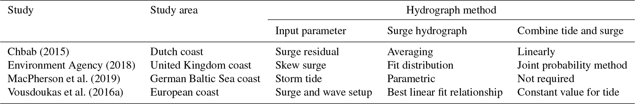
In this section we give an overview of four hydrograph-generating methods. The reason for including these studies on hydrographs in this review, from the wide variety of studies that exists on this topic (e.g. Sebastian et al., 2014; Chbab, 2015; Environment Agency, 2018; MacPherson et al., 2019; Vousdoukas et al., 2016a; Xu and Huang, 2014; Salisbury and Hagen, 2007), is that they all have a clearly distinct methodology. Based on this review, we can select the hydrograph-generating method that best fits our study goals. All four methods use multi-year water-level time series from tide gauge stations or model simulations as input, but they differ in terms of input parameter used, the way the surge hydrograph is computed, and how tide and surge levels are combined. Table 1 summarizes the main characteristics of the four methods.

Table 1 Main characteristics of the four hydrograph methods.

The first method by Chbab (2015) starts by computing the residual water level. The surge residual is the difference between the predicted tide and the storm tide level (Fig. 1). Predicted tides are estimated by harmonic analyses to determine the amplitude and phase of the different tidal constituents. To define the surge hydrograph, events are selected from the residual time series by means of the peaks-over-threshold (POT) method using 1.5 m as a threshold. A 48 h time window lasting from 24 h before until 24 h after the surge maximum is extracted. The final step to obtain the surge hydrograph is normalizing and averaging all 48 h time series of surge levels. To test the sensitivity of the surge hydrograph to the chosen parameters, a sensitivity analysis is performed. They conclude that the upper 50 % of the normalized surge height (normalized surge height > 0.5) is not affected when either the threshold or time window length is increased or decreased. This is an important finding because it indicates that the surge hydrograph is most robust close to the time of high water when defence exceedance is most likely (Santamaria-Aguilar et al., 2017; Quinn et al., 2014). However, a longer time window (of e.g. 72 or 96 h) results in a longer base duration. The argument given for using a 48 h time window is that 48 h is the typical duration of a storm along the Dutch coastline. The surge hydrograph is added linearly to the average tidal cycle where the surge maximum is assumed to coincide with the tide maximum. To generate a hydrograph corresponding to a specific RP, the unitless surge hydrograph is scaled to a certain water level. For example, if the average maximum tide is 1 m and the 100-year storm tide is 3 m, the surge hydrograph is multiplied by 2. In areas with a large tidal range and a wide and shallow continental shelf, tide–surge interaction may induce a time offset between the two maxima (Fig. 1). For example, in the North Sea the surge maximum generally occurs 2.5 h before the tidal maximum (Chbab, 2015; Horsburgh and Wilson, 2007). This is because a storm surge increases the depth and thereby modulates the influence of bottom friction and the speed of the tidal wave (Pugh, 1996; Rego and Li, 2010). The time offset can be taken into account by computing the time offset between the surge and tidal maxima for all surge events above the POT 99th percentile (POT99). Subsequently, the average offset is used to shift the surge time series relative to the tidal maximum.

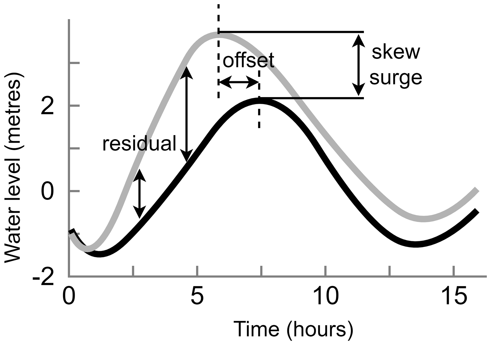
Figure 1 Schematic of the residual, offset, and skew surge. Time series of the tide (grey line) and the tide including meteorological effects (black line) are shown.

The second method, developed by the UK Environment Agency (2018), starts by computing the skew surge. Skew surge (Fig. 1) refers to the difference between the maximum storm tide level and maximum tidal level within a tidal cycle, irrespective of their timing (Williams et al., 2016). An important reason for using skew surge instead of the surge residual is that the latter can arise due to tide–surge interaction (Idier et al., 2019). In contrast to the surge residual, for the skew surge there is no need to account for timing offsets, apart from some locations where a dependency between skew surge and high tidal levels is observed (Santamaria-Aguilar and Vafeidis, 2018). To generate the skew surge hydrograph, the 15 most extreme skew surges are selected. An argument for selecting this number of events is not given. Both the high and low water skew surge values are extracted for each storm event. Subsequently, the high and low water skew surge values are interpolated to a 15 min time series and normalized. Then, the duration of each of the 15 surges at particular percentiles (i.e. 10 %, 20 %, and so on) is calculated. The maximum duration at each percentile is used to compute the skew surge hydrograph. The study by the UK Environment Agency does not combine the skew surge hydrograph with tidal-level time series.

The third method by MacPherson et al. (2019), which further developed the method from Wahl et al. (2011, 2012), starts by identifying storm tide events. To do this, a POT method is used. Using POT is preferred over annual maxima because the number of events extracted is typically higher with POT, resulting in a more robust representation of the local storm tide characteristics in the hydrograph. Then, each event is characterized through a parameterization scheme. A total of 17 parameters are calculated, such as peak water level, event duration, and the flow (rising limb) and ebb (falling limb) curve shape. Subsequently, synthetic hydrographs are generated through Monte Carlo simulations using the obtained parameters. This means that for a single return period multiple storm tide hydrographs are available with different shapes but the same maximum water level.

The fourth method by Vousdoukas et al. (2016a) starts by computing the high tide water level (HTWL). The HTWL is calculated as a constant water level that consists of the mean sea level (MSL) and the maximum tide elevation taken from a 10-year time series. The assumption that the maximum high tidal level occurs along the entire duration of the event, thereby neglecting tidal variations, can significantly overestimate the water level in places with large tidal variability, such as north-western Australia. The HTWL is then combined with time-varying storm surge levels and wave setup to obtain total water levels. Time series of storm surge levels (1979–2014) are taken from Vousdoukas et al. (2016b) and wave setup is approximated by 20 % of the significant wave height, both based on the ERA-Interim global climate reanalysis (Dee et al., 2011). To obtain information about the temporal evolution of an extreme event, extreme events are identified in the available time series of surge and wave setup. For each identified event the duration and peak water level are extracted. Subsequently, a best-linear-fit relationship between the duration and peak water level is estimated. To conclude, the combined hydrograph consists of the HTWL combined with a symmetric triangle-shaped time series on top of it, representing the surge and wave setup for a certain return period.

Comparing the four methods, we find that the hydrograph-generating methods that are developed for application at smaller scales are tailored towards the local water-level characteristics. This makes them less suitable for application at larger scales. For example, in the study by Chbab (2015), a threshold of 0.5 m is used to identify extreme surge events in time series. However, at the global scale surge levels exceeding 0.5 m do not occur in some regions such as the south of the Caribbean. The hydrograph-generating method developed by the UK Environment Agency (2018) is developed for regions that experience a substantial tidal range such as the UK, as it is based on skew surge values. However, the complete global coastline does not experience such high tides. In addition, MacPherson et al. (2019) developed a method that is applicable in areas with a small tidal range, making it well suited for the German Baltic Sea coast and larger scales such as the entire Baltic Sea but inapplicable at continental to global scales. The last study that we discussed (Vousdoukas et al., 2016a) takes a more simple approach to define hydrographs for continental Europe. The tidal component is represented by a constant value and is combined with a triangle-shaped time-varying storm surge. Overall, the study by Vousdoukas et al. (2016a) is a step towards modelling inundation at larger scales using hydrographs. However, substantial improvements can be made to the hydrograph-generating method. To this end, we will build on Chbab (2015) because, most importantly, the method used in this study does take a time-varying surge and tide component into account. In addition, instead of representing the surge by a triangle shape in the combined hydrograph like Vousdoukas et al. (2016a), the method from Chbab (2015) allows the rising and falling limb of the hydrograph to have different shapes. This results in a more accurate representation of the shape of the storm surge in the combined hydrograph. It is especially important that the hydrograph represents the water level correctly close to high water when defence exceedance is most likely and because the water will propagate further inland if the water level is elevated for a longer period of time (Santamaria-Aguilar et al., 2017; Quinn et al., 2014).

3 Methods

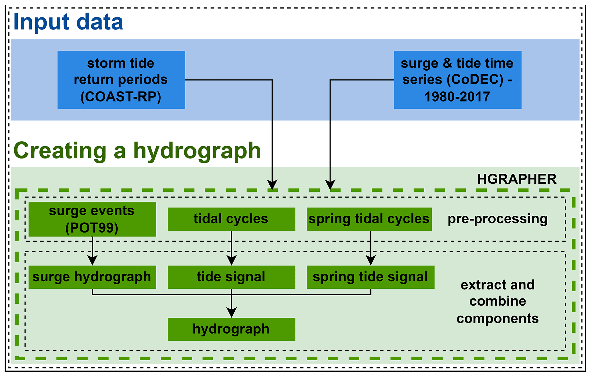
Figure 2 summarizes the main steps of the HGRAPHER hydrograph-generating model. Storm tide levels, tidal time series, and storm tide RPs are used as input. First, extreme events are identified in the surge time series and used to compute a normalized surge hydrograph. Second, the average tide signal is computed from the tidal time series, Third, the hydrograph is generated by combining the average tide signal with the normalized surge hydrograph. To create the final hydrograph, this generic shape is scaled to an absolute water-level height for specific RPs based on a global coastal dataset of storm tide return periods (COAST-RP; Dullaart et al., 2021b).

Figure 2 Modelling framework.

3.1 Input data

Time series of storm tides (1980–2017) at a 10 min interval from 23 226 output locations are taken from the Coastal Dataset for the Evaluation of Climate Impact (CoDEC)–ERA5 dataset (Muis et al., 2020). The CoDEC-ERA5 dataset was generated by forcing the 2D depth-averaged hydrodynamic Global Tide and Surge Model (GTSM) with wind and pressure fields from the ERA5 climate reanalysis (Hersbach et al., 2019). GTSM forced with ERA5 has shown to accurately simulate maximum surge heights of historical TC and ETC events (Dullaart et al., 2020). In addition, a comparison between modelled and observed annual maxima showed a mean bias of −0.04 m (with a standard deviation of 0.32 m) (Muis et al., 2020). Overall, the time series of surge and tidal levels from the CoDEC-ERA5 dataset are of good quality and therefore valid input data to HGRAPHER. The surge time series are computed as the difference between a storm tide simulation and a tide-only simulation. As a result, the surge time series include non-linear tide–surge interaction effects (Horsburgh and Wilson, 2007). The output locations are located at every 50 km along the coastline. In addition, the locations of tide gauge stations are included. In order to scale the hydrograph to a storm tide level that corresponds with a certain RP, we use storm tide RPs from the global COAST-RP dataset (Dullaart et al., 2021b). In contrast to other global storm tide RP datasets, COAST-RP explicitly takes into account low-probability high-impact TCs (Dullaart et al., 2021a) by making use of 3000 years of synthetic TC tracks from the STORM dataset (Bloemendaal et al., 2019).

3.2 Creating a hydrograph

3.2.1 Surge hydrograph

The following procedure is used for each of the 23 226 output locations individually. To generate a hydrograph of the surge, we start with extracting independent extremes from the surge time series based on the peaks-over-threshold (POT) method. Using the POT method for selecting extremes is preferred over annual maxima, as the latter could result in excluding extreme events that happened in the same year. We use the 99th percentile over the complete time series as a threshold, and we select peaks that are at least 72 h apart to ensure independent events (Wahl et al., 2017; Vousdoukas et al., 2016b; Haigh et al., 2016). The threshold results in the selection of on average one surge event per year and 40 events over the full time series. Setting the threshold is a trade-off between having an event set of sufficient size to compute a representative average shape without including too many relatively small surge events that would too strongly affect the resulting shape (see Sect. 4.4). For each selected surge event, we first extract the time series from 36 h before, until 36 h after the peak (Fig. 3a). Second, each 72 h surge event is normalized (i.e. dividing each surge level by the peak) such that the maximum surge value is equal to 1 (unitless). Third, we combine the selected surge events to calculate the average surge hydrograph. This is done by determining the time (relative to the peak) at which a specific surge height (from 0 to 1 with increments of 0.01) is exceeded. As an example, in Fig. 3a we show that for one surge event the exceedance time at a normalized surge height of 0.25 is 14.0 h before and 26.0 h (16.0 + 10.0) after the surge maximum occurred, as indicated by the black arrows. Then, for each normalized surge height the average exceedance time is computed, similarly to Chbab (2015), resulting in an average curve. Because the shape of the rising and falling limb of the surge can differ, the exceedance time is calculated separately for each, and they are subsequently merged into the final average surge hydrograph.

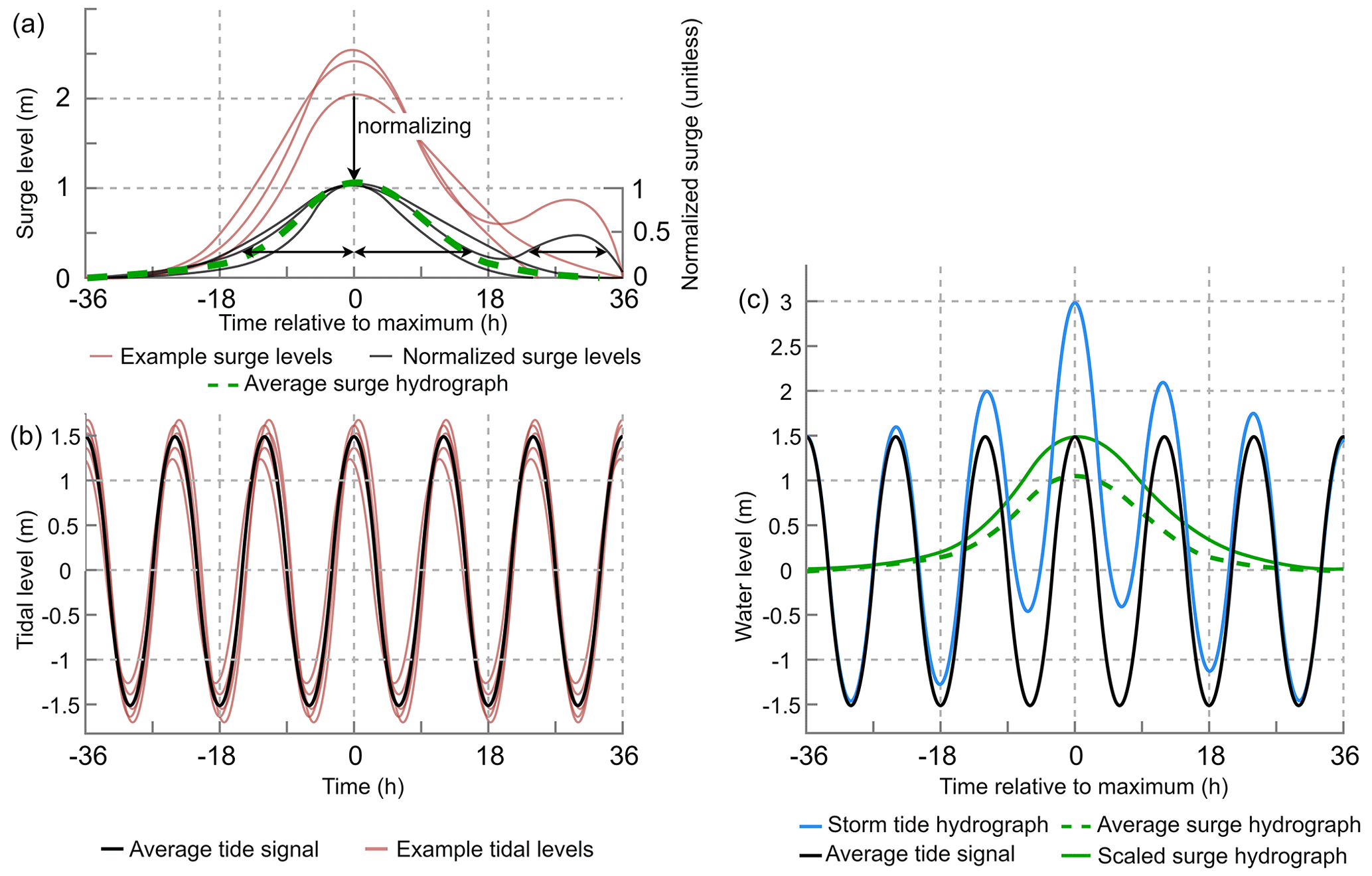
Figure 3 Visualization of the steps leading to the storm tide hydrograph of a hypothetical 1-in-100-year event of 3.0 m with the (a) surge hydrograph, where the black arrows indicate the period over which a normalized surge height of 0.25 is exceeded. Note that for the falling limb we take the sum of the two time periods for which this is the case. (b) Average tide signal and (c) storm tide hydrograph. The average surge hydrograph is scaled to 1.5 m such that the combined water level equals the 1-in-100-year storm tide level of 3.0 m.

3.2.2 Average and spring tide signal

Next, we combine the surge hydrograph with the average tide signal (Fig. 3b). To create a curve representing the average tide signal we take three steps. First, we split the tidal series from the period 1980–2017 up into segments that are each 24 h and 50 min long. The start and end times of the tidal cycles are selected from the tide time series by searching for a minimum around 24 h and 50 min after the previous low tide. The segment length is based on the phase of the M2 tidal component, which is equal to a lunar day (24 h and 50 min). At most locations around the world the M2 is the main tidal component. Second, we compute the mean over all tidal segments to obtain the average tide segment. Third, we duplicate the average tide segment to obtain a longer tidal time series, which we refer to as the average tide signal.

In addition, we extract the spring tide signal because a storm surge event happening at spring tide can result in a very different shape of the hydrograph. The spring-neap tide cycle takes 2 weeks. To extract the average spring tide signal, we first search for the highest tide every 2 weeks. Second, we select 72 h of the tidal time series before and after the spring tide maximum. This procedure is repeated for the available time series of the tide (1980–2017), after which we compute the mean over all spring tides to extract the average spring tide signal.

3.2.3 Storm tide hydrograph

The surge hydrograph is combined with the average tide or spring tide to create a storm tide hydrograph (Fig. 3c). In theory the surge maximum can coincide with any tide. However, in shallow regions the timing will be influenced by interaction effects between the surge and the tide, which result in a phase difference. This is for example the case in the North Sea where the tidal wave will start travelling faster under storm conditions due to the increased water level which reduces the bottom friction (Horsburgh and Wilson, 2007; Resio and Westerink, 2008). To determine whether a typical time offset between the surge and tide should be taken into account, we extract the distribution of the timing offset between the surge and tidal maximum during the most extreme surge events (POT99). For most locations around the globe, the distribution of the timing offset does not show a clear signal (see Sect. 4.4). Therefore, we assume that the surge and tidal maximum coincide. With HGRAPHER a hydrograph can be generated for a total water level of interest. In this study we use storm tide levels corresponding to a 100-year return period (RP100) because this is an often-used coastal protection standard (Lamb et al., 2018; FEMA, 1968). If, for example, the RP100 storm tide level is 3.0 m and the average high tide is 1.5 m, this means the unitless average surge hydrograph has to be scaled up to 1.5 m such that the maximum surge plus the maximum tide are equal to 3.0 m (Fig. 3c).

4 Results

4.1 Storm surge hydrographs

For each output location from the CoDEC-ERA5 dataset, a surge hydrograph is generated. For illustration, results are shown for La Rochelle in France and Marco Island in the United States (Fig. 4a and b). We find a storm surge duration (i.e. the time over which the normalized surge height is above zero) of 54 h in La Rochelle and 42 h in Marco Island. Other studies find comparable storm surge durations of 40 h for Hoek van Holland and 45 h for Den Helder in the Netherlands (Chbab, 2015) and between 40 and 70 h for the German Baltic Sea coast (MacPherson et al., 2019). The difference in storm surge duration between La Rochelle and Marco Island is likely caused by the different types of storms occurring in these regions. TCs can cause a fast shift from onshore to offshore winds when making landfall, which results in the surge becoming negative in just a couple of hours. Hurricane Irma is an example of a TC that made landfall near Marco Island and caused such a fast shift in surge levels. The normalized surge level time series have a strong irregular behaviour. This originates from the fact that the surge time series are obtained by subtracting tide-only simulations from total water-level simulations (including tidal and meteorological forcing). Therefore, the surge time series are the residual water levels that include tide–surge interaction effects, and we believe this partly explains the irregular behaviour. Differences in the evolution of storms over time can also contribute to the variability observed at the different time steps of the normalized surge levels, particularly in areas that are affected by TCs and ETCs, as the characteristics of the two types of storms differ considerably (Domingues et al., 2019). In addition, not all 40 events are extreme over their complete lifetime, which means that noise is affecting the lower ends of the hydrograph. Taking the mean over the normalized surge heights removes this irregular shape. At the global scale a distinct pattern shows up in certain regions (Fig. 4c). In Europe for example, the average storm surge duration is substantially lower in the North Sea compared to the Atlantic coastline and the Baltic Sea. Last, we computed the difference in surge hydrograph duration between the 25th and 75th percentile at a normalized surge height of 0.75 (Fig. A1). This can provide some insights into the variability of flood duration, assuming that inundation might start to occur around the 0.75 normalized surge height.

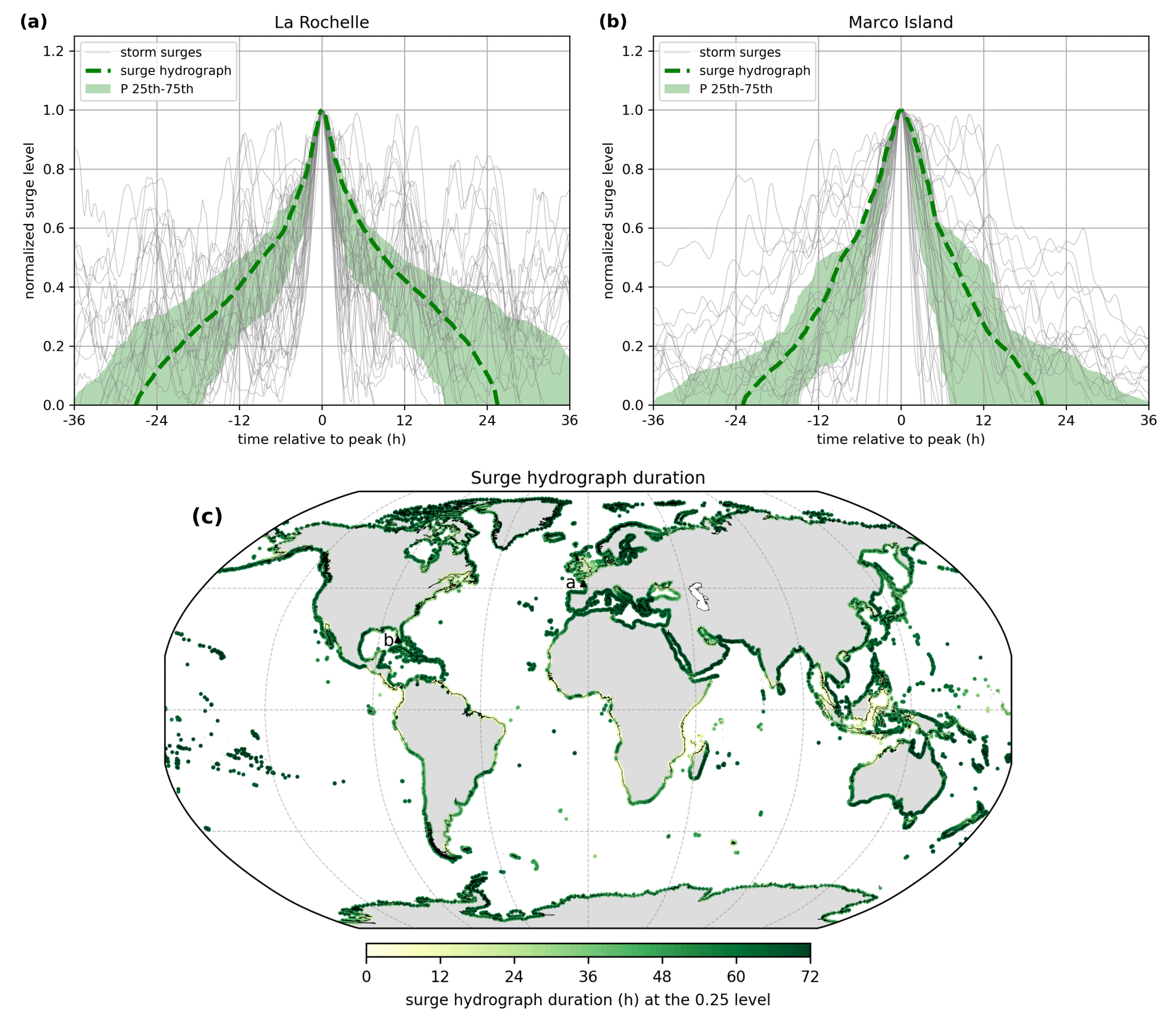
Figure 4 Surge hydrograph (dashed green line) for (a) La Rochelle and (b) Marco Island. Normalized surge levels are shown in grey, and the green shaded area represents the 25th–75th percentile. Panel (c) shows the surge hydrograph duration at 0.25, with the locations of La Rochelle and Marco Island indicated by a and b, respectively.

4.2 Average (spring) tide signal

For each output location the average and spring tide signals are computed. Although the tidal range at La Rochelle is substantially larger than at Marco Island, the general shape of the average tide signal is comparable (Fig. 5a and b). Both locations show a large variation in amplitude between tidal cycles. For spring tide, the variation in the tidal amplitude between the tidal cycles is smaller. Note that the grey shaded area exceeds the red shaded area at both locations during the first and third high tide because the average spring tide signal is computed by taking the average over a 2-week period, while the average tide signal is computed by taking the average over the daily tidal cycle of 24 h and 50 min. Furthermore, the duration of the first and second high and low tide cycle of a tidal day differs at Marco Island. This is caused by the type of tide at this location, which is a mixed semidiurnal tide (i.e. a tidal regime with two high and low tides per tidal day of different size) (Song et al., 2011). Computing the average tide signal can be difficult at locations with a very small tidal amplitude and mixed semidiurnal tide such as Montevideo (Fig. A1). Because of the large number of shapes that the tidal cycles can have here, taking the average will not completely represent all possible shapes. However, because the average high tide values are correctly represented by the average (spring) tide signal, the findings are not affected to a large extent. For La Rochelle the maximum average tide signal increases with 46 % from 1.85 m based on all tidal cycles to 2.70 m when taking the average of the spring tidal cycles. In Marco Island the maximum average tide signal is 0.40 m, and the maximum average spring tide is 0.59 m (+48 %). The larger absolute difference in La Rochelle means that for an extreme storm tide to occur, the timing of the surge maximum relative to the (spring) tide maximum is more important compared to Marco Island. When applying HGRAPHER, it is important to understand the typical characteristics of a storm tide in the area of interest because this information is needed to choose between the average and spring tide signal. For example, in north-western Australia the difference between the maximum average and spring tide signal exceeds 1.5 m (Fig. 5c), indicating that in this region an extreme storm tide is much more likely to occur during spring tide. Therefore, using the average spring tide signal should be considered. At the global scale, the difference between the average and spring tide signal maxima exceeds 0.5 and 1.0 m at 24 % and 3 % of all output locations, respectively.

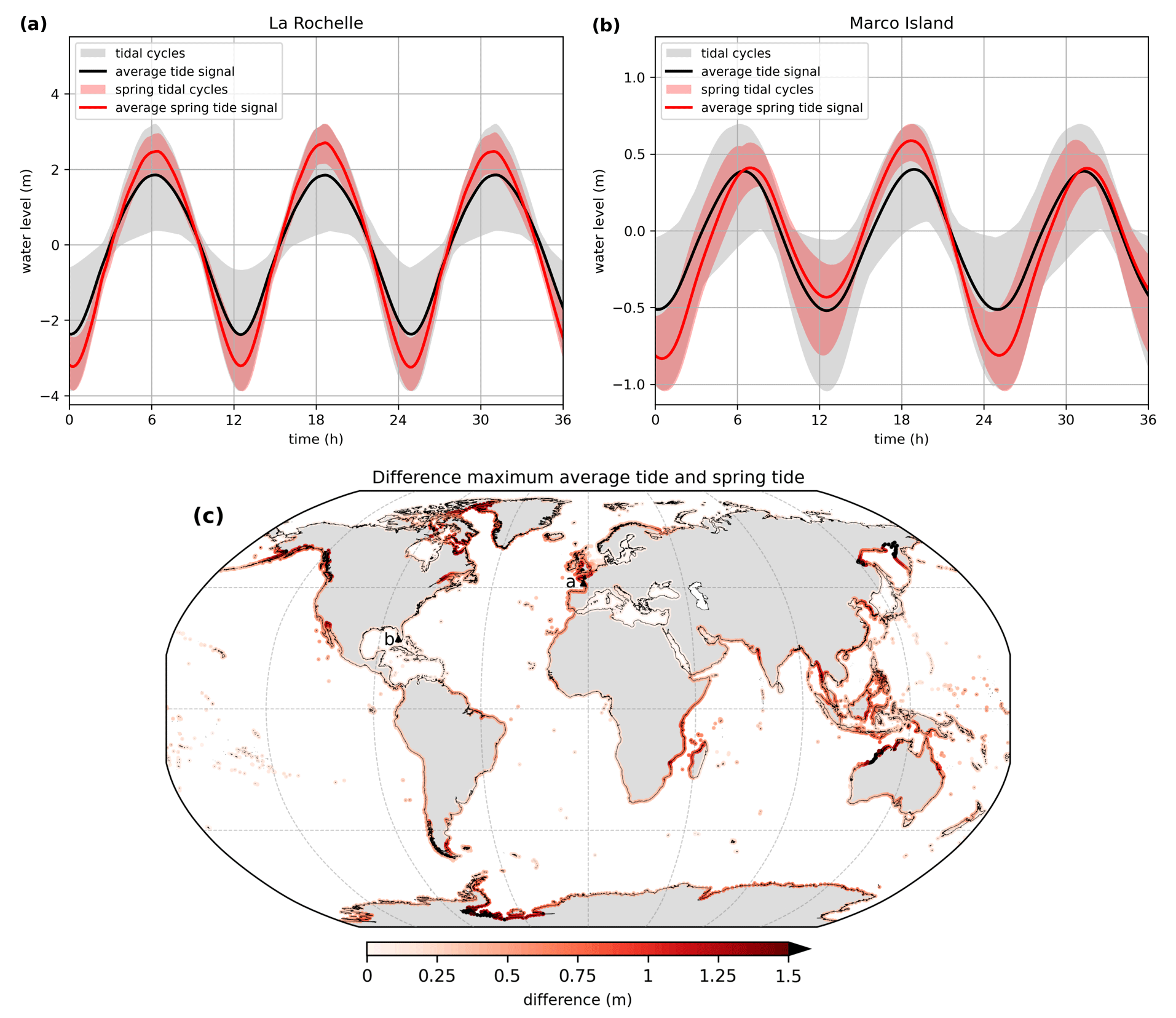
Figure 5 Average tide signal (black line) for (a) La Rochelle and (b) Marco Island. The grey shaded area shows the range of all tidal cycles. The average spring tide signal is shown in red, and the red shaded areas indicate all tidal cycles that are used to compute the average spring tide signal. Panel (c) shows the absolute difference between the maximum average tide signal and average spring tide signal. The locations of La Rochelle and Marco Island are indicated by the letters a and b, respectively.

4.3 Storm tide hydrographs

The surge hydrograph is scaled up to a certain water level and combined with the average tide signal to obtain the storm tide hydrograph (Fig. 6a and b) that corresponds to the 1-in-100-year (RP100) storm tide level from the COAST-RP dataset (Dullaart et al., 2021b). In La Rochelle the RP100 storm tide level is 3.76 m, and the average high tide is 1.85 m. Therefore, the unitless surge hydrograph is scaled up to 1.91 m such that the combined water level equals the RP100 storm tide level. At Marco Island the RP100 storm tide level is 2.18 m, to which the tide contributes 0.40 m and the surge 1.78 m. From the RP100 storm tide hydrograph that we create globally it is possible to deduce the relative contribution of the surge (Fig. 6c). Especially in areas where the maximum spring tide signal substantially exceeds (> 0.5 m) the maximum average tide signal, the surge contribution might be too large compared to observed historical events. This effect is counteracted by the assumption that the surge and tide coincide in time. As a result, a smaller surge is sufficient to get to the desired RP100 storm tide level compared to the situation where a time offset is implemented to combine the average tide signal with the scaled surge hydrograph. Last, the surge hydrographs are based on the surge residual, including tide–surge interaction effects. These interaction effects tend to be positive at low tide and negative at high tide (Horsburgh and Wilson, 2007). As a result, we might overestimate the contribution of the surge to the combined hydrograph at high tide.

Figure 6 RP100 storm tide hydrograph (blue line) for (a) La Rochelle and (b) Marco Island. The average tide signal (black line), average surge hydrograph (green line), and scaled surge hydrograph (dashed green line) are also shown. Panel (c) shows the relative contribution of the surge to the RP100 storm tide hydrograph maximum as a percentage. The locations of La Rochelle and Marco Island are indicated by the letters a and b, respectively.

4.4 Assumptions underlying the hydrograph

HGRAPHER is based on certain assumptions to create the storm tide hydrographs. Here, we aim to better understand how these assumptions influence the results. First, we assume that the POT99 threshold results in the selection of a set of surge events from the residual time series that represents the typical evolution of a surge event at any location. However, using a higher or lower POT percentile to select surge events will give different results, depending on the typical characteristics of a location. We illustrate this using La Rochelle and Marco Island as an example. Using a higher (POT99.5) or lower (POT98) POT percentile does not result in a clearly deviating surge hydrograph at La Rochelle (Fig. 7a). At Marco Island however (Fig. 7b), a clear difference can be observed between the surge hydrographs. Using the higher POT99.5 percentile (i.e. only using the ∼ 20 most extreme surge events) results in a hydrograph that is more narrow and has a shorter duration. This is most likely caused by the different types of storms that occur at Marco Island. Using a higher POT percentile as threshold will result in an event set with a relatively larger share of TCs compared to ETCs. This indicates that surge events caused by TCs are typically shorter compared to ETC-related surge events at Marco Island. Wahl et al. (2011) also showed that the peak of the surge hydrograph can show a dependency to the intensity of the underlying surge events. At the global scale, it can be observed that the surge hydrograph duration (at the unitless 0.5 level) is typically shorter in the Caribbean and north-western Pacific Ocean when only using the more extreme surge events (i.e. POT99.5 relative to POT98) for generating a surge hydrograph (Fig. 7c). Outside TC-prone areas the variability in surge hydrograph duration, either positive or negative, is less pronounced. Overall, to select the best POT percentile to generate the surge hydrograph, knowledge about the local conditions is required. For example, if surge events happen very infrequently (i.e. less than once per year), a percentile higher than POT99 should be used. Correspondingly, in areas where TCs occur, such a higher POT percentile should be chosen if the research focusses on TCs. For this, knowledge about the number of historical TC storm surge events is required. Conversely, if the goal is to create a RP1 storm tide hydrograph, a lower POT percentile is warranted compared to when one is interested in the RP100 storm tide hydrograph.

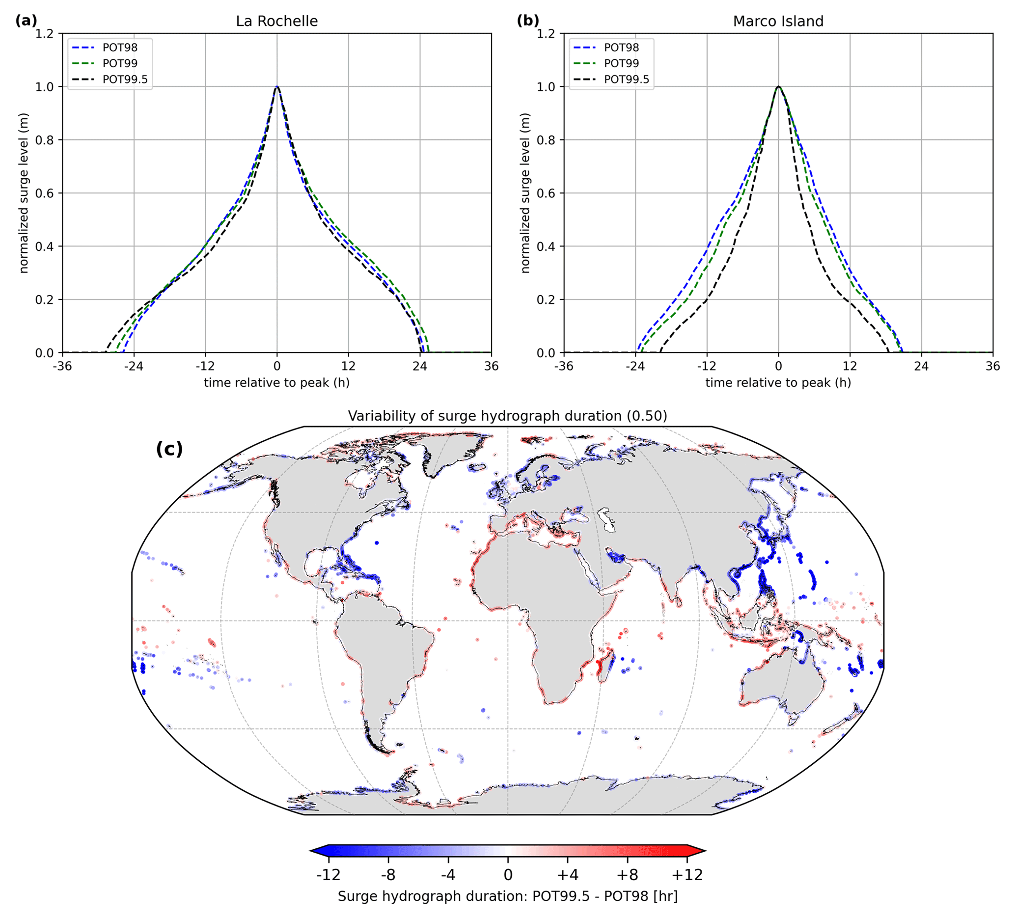
Figure 7 POT99 surge hydrograph (dashed green line) for (a) La Rochelle and (b) Marco Island. The dotted blue and black lines show the average surge hydrograph based on the surge events that exceed the POT98 and POT99.5 percentile. Panel (c) displays the difference in surge hydrograph duration in hours at a normalized surge level of 0.5, computed as POT99.5 minus POT98.

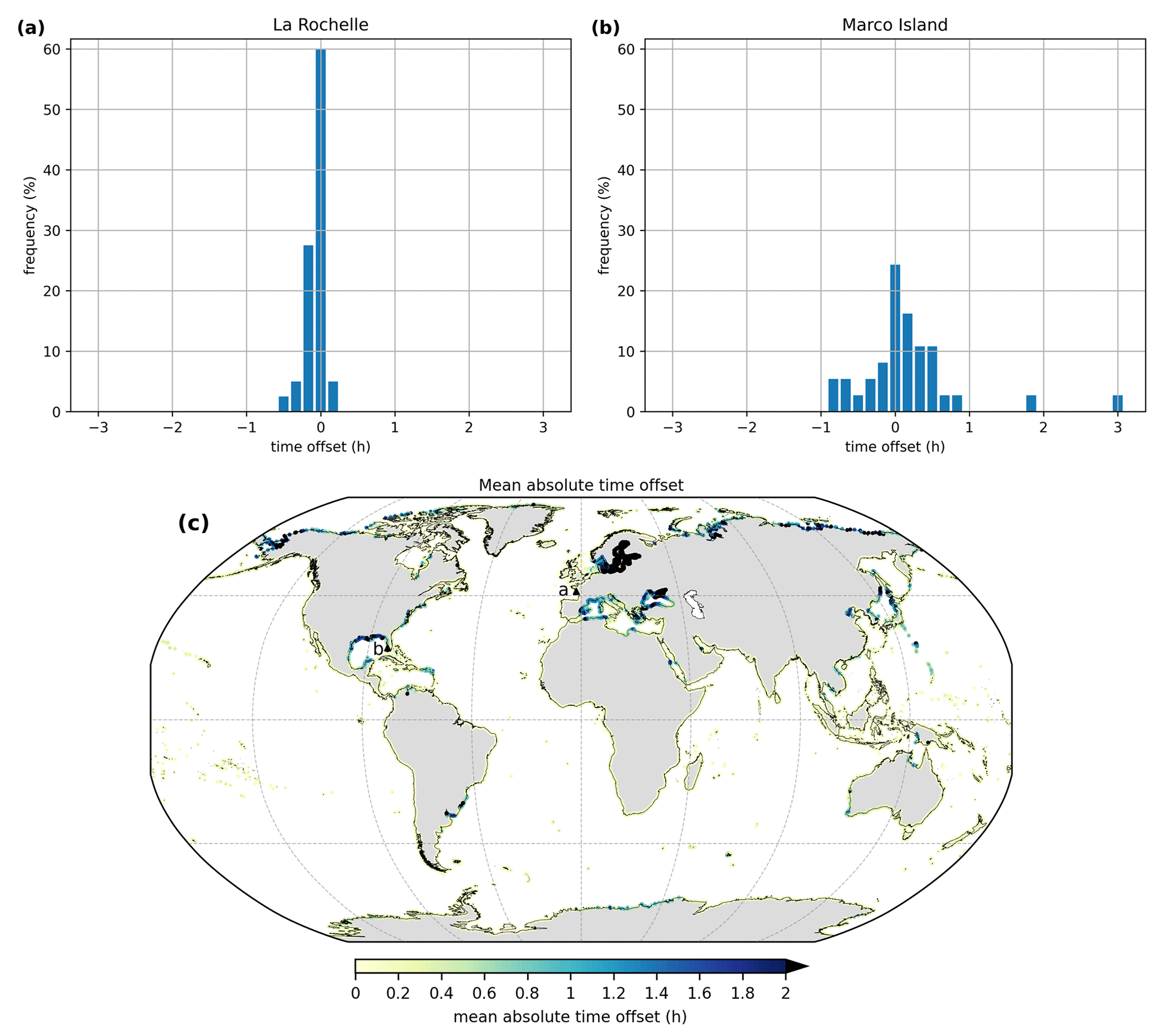
Figure 8 Time offset distribution of the POT99 storm tide maxima relative to astronomical high tide at (a) La Rochelle and (b) Marco Island. Each blue bar represents a 10 min period. Panel (c) shows the mean absolute time offset in hours. The locations of La Rochelle and Marco Island are indicated by the letters a and b, respectively.

Second, when combining the surge hydrograph with the average tide signal we assume that the maxima of the two coincide in time. Including a time offset will lead to a storm tide hydrograph of which the water level is elevated over a longer period of time, potentially increasing the severity of a flood event. To test this assumption we compute the time offset at La Rochelle and Marco Island (Fig. 8a and b), which is defined as the timing of the maximum storm tide relative to astronomical high tide (Fig. 1). What can be observed at both output locations is that the distribution is centred around zero. However, at Marco Island the distribution is more spread out, indicated by a standard deviation of 0.68 compared to 0.13 for La Rochelle. At the global scale, large mean absolute time offsets are observed in areas with either a very small tidal range, such as the Baltic Sea and the Mediterranean Sea, or a diurnal tide regime in combination with large TC-induced storm surges, such as the Gulf of Mexico (Fig. 8c). We show the absolute time offset instead of the actual values because this way all areas where large time offsets occur are revealed, including areas with both positive and negative time offsets. The globally averaged absolute mean offset is 33 min, and the median is 9 min. To conclude, the assumption that the surge and tide maxima coincide is appropriate at most output locations. However, at certain locations it should be considered to include a time offset when creating a storm tide hydrograph.

5 Discussion and conclusion

This study improves the understanding of the duration and shape of extreme sea-level events along the global coastline. It provides a novel global dataset of storm tide hydrographs, which is an important first step in moving away from the planar approach towards dynamic inundation modelling. The open-source HGRAPHER model can generate hydrographs and allows users to create storm tide hydrographs for an RP of interest. Here, we used time series of surge, tide, and storm tide levels from the CoDEC dataset (Muis et al., 2020) as input and generated storm tide hydrographs with a 1-in-100-year return period based on COAST-RP (Dullaart et al., 2021b). Users have multiple options, including (1) using the average tide signal or spring tide signal, (2) defining a POT percentile to select surge events for generating the surge hydrograph, (3) including a time offset for combining the surge hydrograph with the tide, (4) defining for which RP a storm tide hydrograph should be generated, and (5) using other time series or return periods as input data for HGRAPHER.

Several aspects of our methodology could be further improved. First, we use 38 years of surge-level time series that are obtained by subtracting tidal-level time series from the storm tide level. As a result, the surge time series do not only contain the meteorological contribution to the sea level but also contain tide–surge interaction effects (Horsburgh and Wilson, 2007). This could be addressed by using a surge-only simulation, which would not be affected by interaction effects. Another aspect that could be improved is that our analysis is based on a 38-year time series. This provides a limited number of events, specifically for regions that do not regularly experience extremes, such as the equatorial regions. Potentially we could extend our analysis by using a large set of synthetic events, such as those presented for TCs in Dullaart et al. (2021a). For extra-tropical regions, seasonal forecasts could be used to create a large ensemble of events (Haarsma et al., 2016). The advantage of a large set of synthetic events is that it would allow us to assess if hydrographs are different for different RPs. This is currently not possible because of the small sample size.

Second, we do not account for different types of storms. TCs and ETCs have distinct meteorological characteristics, resulting in a different evolution of the water level over time. For example, TCs can have stronger wind speeds and a lower air pressure than ETCs, resulting in a higher storm surge (Keller and DeVecchio, 2016). ETCs on the other hand generally affect a larger coastal area because they are often larger in size than TCs (Irish et al., 2008). The typical radius of a TC is between 100 and 500 km, while for an ETC it is in the range of 100–2000 km. In addition, once TCs move inland the wind direction can become offshore directly at the coast, resulting in a storm surge sign that quickly changes from positive to negative. An example of this is during TC Irma, which made landfall in Florida in 2017 (Cheng and Wang, 2019). A potential direction for future research would be to separate storm surges by type of storm that caused them and develop a surge hydrograph individually for TCs and ETCs. This would require much longer surge time series (representing thousands of years instead of decades) that could be created using, for example, large climate model ensembles (Haarsma et al., 2016) or synthetic tracks of TCs (Bloemendaal et al., 2020).

Third, the average tide signal is computed by taking the average over thousands of tidal cycles with a duration of 1 lunar day, lasting 24 h and 50 min. For the majority of the output locations HGRAPHER correctly extracts the average (spring) tide signal. However, in areas with a mixed tidal regime the daily uneven magnitude of the two high tides is averaged out. This is because over time it alters whether the first or second high tide is the highest tide during that lunar day. Including the mixed tidal regime characteristics at these locations, such as Montevideo (Fig. A2), would result in a more realistic storm tide hydrograph. However, for this to happen multiple storm tide hydrographs that have different shapes but reach the same maximum water level have to be generated. This would make the storm tide hydrograph dataset less easily applicable in large-scale flood hazard assessments.

A final limitation is that our analysis does not include waves. Wave setup can increase storm tide levels at the coast. Therefore, it is often an important component of extreme sea levels, and including a dynamic wave setup component in HGRAPHER is a potential direction for future research. To accomplish this, we could make use of a parametric approach that has been used in previous global-scale studies to obtain estimates of wave setup (Vousdoukas et al., 2018; Kirezci et al., 2020).

HGRAPHER and the global dataset of storm tide hydrographs improve our understanding of the duration and shape of storm tide levels. They provide a basis to move towards more dynamic inundation modelling across different spatial scales, and as a next step, the hydrographs could be applied as boundary conditions in inundation modelling. This way, the time component is taken into account when modelling inundation, which will substantially improve the accuracy of coastal flood hazard assessments across different spatial scales.

Appendix A

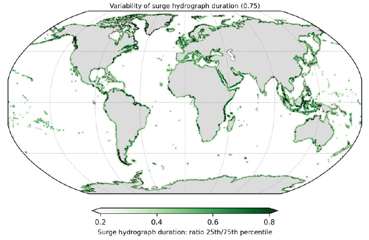
Figure A1 Ratio of the surge hydrograph duration of the 25th and 75th percentile at the normalized surge height 0.75. The ratio is computed by dividing the 25th percentile value by the 75th percentile value.

Figure A2 Average tide signal (black line) for Montevideo. The grey shaded area shows the range of all tidal cycles. The average spring tide signal is shown in red, and the red shaded area indicates all tidal cycles that are used to compute the average spring tide signal.