Estimating the likelihood of roadway pluvial flood based on crowdsourced traffic data and depression-based DEM analysis

Water ponding and pluvial flash flooding (PFF) on roadways can pose a significant risk to drivers. Furthermore, climate change, growing urbanization, increasing imperviousness, and aging stormwater infrastructure have increased the frequency of these events. Using physics-based models to predict pluvial flooding at the road segment scale requires notable terrain simplifications and detailed information that is often not available at fine scales (e.g., blockage of stormwater inlets). This brings uncertainty into the results, especially in highly urbanized areas where micro-topographic features typically govern the actual flow dynamics. This study evaluates the potential for flood observations collected from Waze – a community-based navigation app – to estimate the likelihood of PFF at the road segment scale. We investigated the correlation of the Waze flood reports with well-known flood observations and maps, including the National Flood Hazard Layer (NFHL), high watermarks, and low water crossings data inventories. In addition, highly localized surface depressions and their catchments are derived from a 1 m resolution bare-earth digital elevation model (BE-DEM) to investigate the spatial association of Waze flood reports. This analysis showed that the highest correlation of Waze flood reports exists with local surface depressions rather than river flooding, indicating that they are potentially useful indicators of PFF. Accordingly, two data-driven models, empirical Bayes (EB) and random forest (RF) regression, were developed to predict the frequency of flooding, a proxy for flood susceptibility, for three classes of historical storm events (light, moderate, and severe) in every road segment with surface depressions. Applying the models to Waze data from 150 storms in the city of Dallas showed that depression catchment drainage area and imperviousness are the most important predictive features. The EB model performed with reasonable precision in estimating the number of PFF events out of 92 light, 41 moderate, and 17 severe storms with 0.84, 0.85, and 1.09 mean absolute errors, respectively. This study shows that Waze data provide useful information for highly localized PFF prediction. The superior performance of EB compared to the RF model shows that the historical observations included in the EB approach are important for more accurate PFF prediction.

1 Introduction

This study developed and tested a new data-driven framework for short-term flash flood likelihood estimation at the scale of road surface depressions based on crowdsourced traffic data. Flash flooding is considered one of the most hazardous natural disasters that affect people worldwide (Kousky, 2018). Analysis of flash floods over the contiguous United States shows that flash flood frequency and property damage have increased in the past 2 decades (Ahmadalipour and Moradkhani, 2019). Pluvial flash flooding (PFF) is defined as localized floods caused by an overwhelmed natural or engineered drainage system (Carter et al., 2015; Rosenzweig et al., 2018). PFF can reduce the reliability of roadway networks by decreasing capacity, increasing travel time, reducing safe speed, and increasing accident risks and deaths through lane submersion (Agarwal et al., 2005; Suarez et al., 2005; Smith et al., 2004).

Most urban flood studies have focused on fluvial and coastal flooding rather than PFF. Rosenzweig et al. (2018) identified three reasons for pluvial flooding being less studied: (1) it is assumed that stormwater infrastructure, such as sewers, culverts, and pumps, are sufficient to prevent pluvial flooding, (2) pluvial flooding is believed to be a nuisance with minimal impacts, and (3) lack of monitoring data to capture short-duration precipitation over small urban watersheds.

In the past, stormwater minor system (curbs, gutters, inlets, pipes, and channels) have been designed to minimize nuisance hazards associated with a 10-year or less recurrence interval rainfall (US Department of Transportation FHWA, 1979). More recent roadway facilities are designed and evaluated for 50 and 100-year events (Mark and Marek, 2011), but in older urban areas undersized conveyance systems remain (Jack et al., 2021). With climate change, growing urbanization, and increasing imperviousness, the frequencies of extreme rainfall events and nuisance flooding are increasing (United Nations, 2019; Hemmati et al., 2021, 2020), leading to increased risks from pluvial flooding. Mobility disruption is a noticeable consequence of PFF (Douglas et al., 2010; Yin et al., 2016; Coles et al., 2016; Li et al., 2018). For example, Pregnolato et al. (2017) estimated that a driver facing 10 cm of standing water must not drive faster than 40 km h⁻¹ to maintain safe driving, stopping, and steering without loss of control. Furthermore, according to the National Weather Service (National Weather Services, 2022) 30 cm of standing water can be sufficient to float most cars.

In order to warn drivers about rapidly changing flash flood conditions, high-resolution predictive models are needed at navigational scale (road segment and intersection). Simplified terrain models, such as the rapid flood spreading model (RFSM; Lhomme et al., 2008), height above nearest drainage model (HAND; Nobre et al., 2011), and hierarchical filling and spilling models (Zhang and Pan, 2014; Chu et al., 2013; Wu et al., 2019; Samela et al., 2020) can estimate inundation extent in less complex terrains where the dynamics of flow, velocity, and momentum are negligible (Teng et al., 2017). Statistical methods are also able to predict flooding by analyzing historical observations, however, since they learn from the past, updating procedures are required to make them adaptive to accelerated future changes as they are built upon the assumption that similar conditions in the future will cause flooding. A notable advantage of statistical PFF models is their ability to capture impacts of unobserved variables and uncertainties from historical observations, as well as the ability to rapidly update the models as new data become available and system dynamics change. Haghighatafshar et al. (2020) suggested that designing stormwater infrastructure based on storm recurrence intervals is ambiguous, while statistical models can provide the basis of a more resilient system by taking uncertainties of vulnerability and hazard of pluvial flooding into account. Many studies have investigated statistical flood modeling to predict flooding by applying statistical and machine learning methods such as classification models, Bayesian frameworks, and random forest models (Tien Bui and Hoang, 2017; Solomatine and Ostfeld, 2008; Tehrany et al., 2013; Zahura et al., 2020). Other studies have combined deterministic physics-based models with statistical models for forecasting applications (Li and Willems, 2020; Zhao et al., 2018).

Empirical and data-driven models require flooding observation data with high spatiotemporal resolution. The average duration of flash flooding events in the United States has been 3.5 h during the last two decades (Ahmadalipour and Moradkhani, 2019), limiting the applicability of aerial imagery to obtain sufficiently frequent flash flooding observations. To fill this data gap, there is increasing interest in the application of newer “crowdsourced” data into flood modeling, monitoring, and impact assessment (Molinari et al., 2018; Gaitan et al., 2016; See, 2019; Assumpcao et al., 2018; Praharaj et al., 2021a; Helmrich et al., 2021; Zhu et al., 2022; Liu et al., 2021; Schnebele et al., 2014). Previous crowdsourced flood data studies have involved engaging citizens in collecting four types of data: streamflow or rain gauge readings, videos, text messages, and image postings (Li and Willems, 2020; Assumpcao et al., 2018; Zhu et al., 2022; Liu et al., 2021; Schnebele et al., 2014; Le Coz et al., 2016; Smith et al., 2017; Cervone et al., 2015; Wang et al., 2018; Pereira et al., 2020; Moy De Vitry et al., 2019). Also, Zhu et al. (2022) and Liu et al. (2021) applied artificial intelligence techniques to extract flooding waterlogging from microblog information shared in crowdsourcing apps. A big challenge in using crowdsourced data is identifying the accurate location and flood extent from posted pictures, videos, and texts. However, even with the challenges mentioned above, researchers have concluded that integrating crowdsourced data into flood models improves the overall performance and timeliness of forecasts, hence increasing flood hazard awareness (Assumpcao et al., 2018; Goodrich et al., 2020).

The majority of studies have implemented crowdsourced data into physics-based models as complementary data for model setup, calibration, validation, and data assimilation (Zahura et al., 2020; Assumpcao et al., 2018; Smith et al., 2017). However, physics-based models can be limited in flood prediction at road segment scales due to highly complex and interconnected variables that contribute to flooding in urban environments (Coles et al., 2016; Rafieeinasab et al., 2015). Micro-topographic features, steep slopes, and varying surface materials can generate different types of flow regimes at small spatial scales. Dual-drainage hydrodynamic models that couple equations for the underground sewer system and surface flow require detailed layouts of urban drainage systems that can be of varying quality, particularly in older urban areas where PFF is most prevalent (Haghighatafshar et al., 2020; Smith et al., 2017; Sadler et al., 2018; Berndtsson et al., 2019). Finally, catchments that drain into roadways are often very small and ungauged, leading to further uncertainties in estimating road inundation (Versini et al., 2010). Hence accurate high-resolution real-time physics-based hydrodynamic modeling in urban areas is computationally extensive and rarely considered feasible (Mignot et al., 2006; Sanders et al., 2020).

In this study, we address these gaps and limitations of PFF probability estimation on roadways by incorporating crowdsourced navigation data from the Waze navigation app as highly localized flood observations into high-resolution data-driven models that can be updated and implemented rapidly to provide near-real-time navigational warnings. The framework developed has three steps. In the first step, road surface depressions and their upstream catchments are delineated from a high-resolution digital elevation model using simplified flow-routing and hierarchical fill spill approaches. In the second step, two statistical and machine learning models – empirical Bayes (EB) and random forest (RF) – are developed and tested to predict PFF frequency using roadway, catchment, depression, and rainfall characteristics. In the third step, the probability of roadway flooding and flood maps are generated that could be disseminated to navigation software. To our knowledge, this study is the first to develop real-time PFF likelihood maps at road segment scales using data-driven models and crowdsourced traffic data. With the widespread use of smartphones and crowdsourced applications, this study shows the benefits of integrating crowdsourced data and statistical modeling approaches into roadway flood awareness and management systems.

2 Methodology

The three steps of the framework developed are shown in Fig. 1. The first step involves data preprocessing to create the dataset needed for modeling. The second step fits statistical and machine learning models to the historical dataset, and the third step performs the roadway flooding likelihood estimation for future storms. These steps are described in more detail in sections below.

Figure 1 Methodology framework (basemap from ESRI-2021).

2.1 Step I: Preprocessing

The dataset preprocessing in Step I includes three primary components that are described in detail in the sub-sections below and depicted in Fig. 1. First, road surface depressions and their upstream catchments are delineated. Second, storm events and their characteristics are determined from continuous rain gauge observations; third and last, flood alerts are assigned to corresponding depressions and storm events.

2.1.1 Depression extraction

The first step of data preprocessing is to find road surface depressions that are prone to PFF. Generally, surface depressions are defined as the difference between the hydrologically conditioned digital elevation model (DEM) (Lindsay and Dhun, 2014) and the raw DEM. In hydrologically connected DEM elevations internally draining sinks are raised to form a flat area that can drain to downstream. Locating surface depressions in a highly urbanized terrain is challenging due to micro-topographic and underground features (such as curbs, stormwater inlets, etc.) that determine the actual flow path. In addition, using a high-resolution DEM (1 m) introduces hierarchical depressions with different orders of magnitude in a spatial scale, from highly localized (minor pits) to surface depressions that cover more than one neighborhood (residual depressions). Therefore, a nested hierarchy of depressions must be considered to extract depressions compatible with urban features.

In this paper, the “sink evaluation” tool of the Arc Hydro toolbox (Djokic et al., 2011) is utilized to extract a nested hierarchy of surface depressions. The sink evaluation tool scans the bare-earth DEM (BE-DEM) and characterizes low-lying cells. The process of local depression extraction is an iterative process that examines each sink, raises the elevation of low-lying cells to fill the sink, and then reapplies the process on the resulting DEM. This procedure is depicted in Fig. 2. In the first sink evaluation step, Level-1 depressions are delineated and raised (Fig. 2a). In the second step, the DEM resulting from the first level fill (Fig. 2e, red areas) is evaluated and Level-2 depressions are delineated. This process can be repeated until the area is fully hydrologically conditioned and no higher-level depressions remain. The number of steps required in this process is dependent on the resolution of the DEM and the complexity of the depressions in the landscape.

Figure 2 Hierarchical filling of surface depressions (basemap from ESRI-2021).

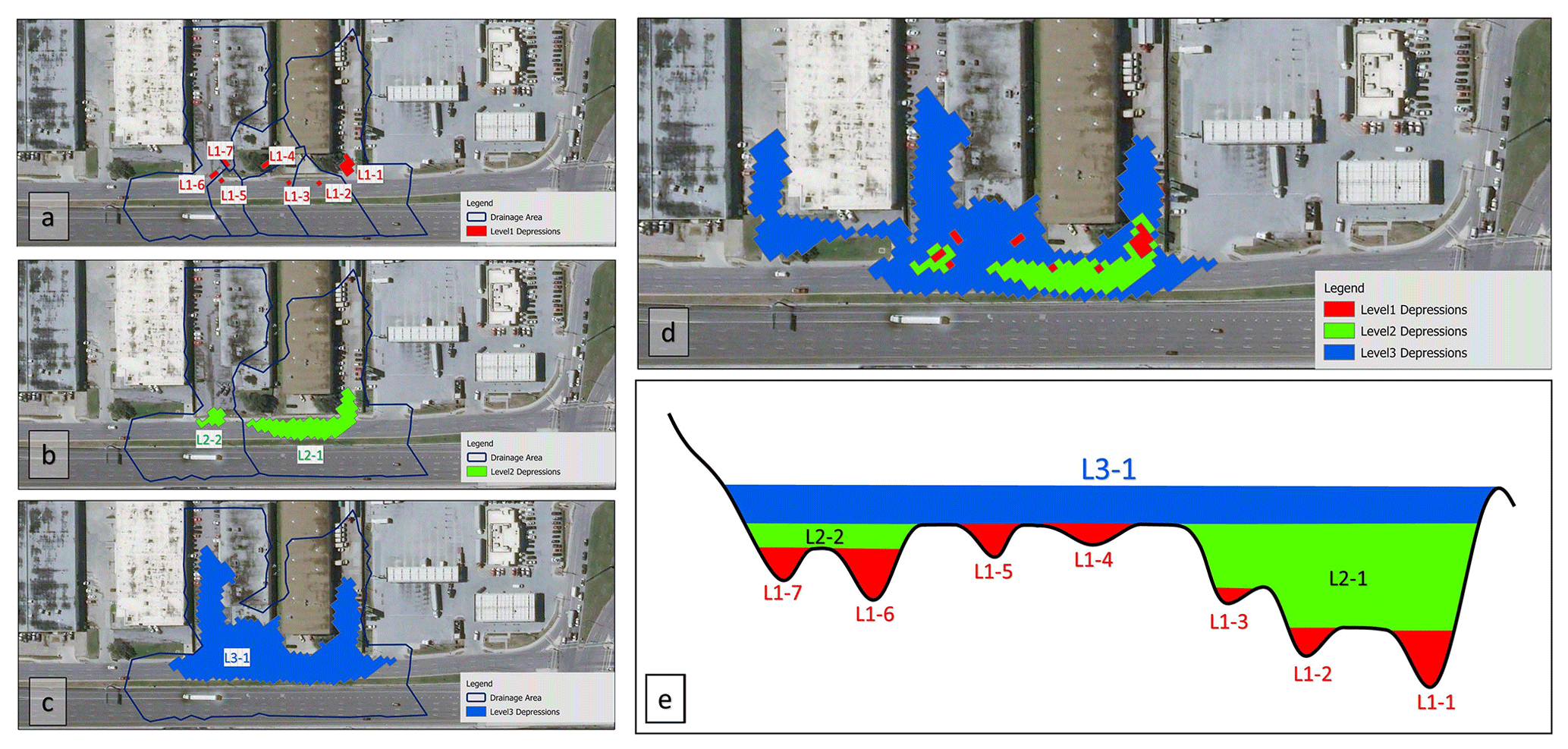
Due to the complexity of urban terrain, the spatial scale of depressions at each hierarchy level is quite variable, and depressions at the same level can be as large as a neighborhood or as small as a pothole. Initially, depressions at all hierarchical levels were extracted. Since 15 cm of standing water has minimal impact on most cars (National Weather Services, 2022), depressions with maximum depth smaller than 15 cm are removed from further analysis. Next, those depressions that best represent and align with urban topographic features that block flow, such as roadway curbs and gutters, are manually selected as flood-prone depressions. Flood-prone depressions are then selected by examining overlays of the depressions and Waze flood reports, as well as the areas of depressions and road surfaces that the depression covers. Heuristics for this procedure are presented in detail in Sect. 2.1.5. Figure 2e shows 10 depressions (L1-1 to L1-7, L2-1, L2-2, and L3-1) extracted on a road segment with three depression levels. Level-1 depressions and L2-2 appear as single cell or too small pits on the road surface to cause traffic disruption. However, L2-1 aligns with road curbs and gutters and could cause traffic disruptions by covering a large area and all lanes of the roadway. Therefore, L2-1 is manually selected as the smallest depression that is prone to PFF and could affect traffic flow on this road segment. (Note that L3-1 includes L2-1; hence, it will be filled only after L2-1 has filled and disrupted traffic flow already. Hence, L3-1 does not need to be included in the model for traffic navigation purposes.)

2.1.2 Physical depression and catchment descriptors

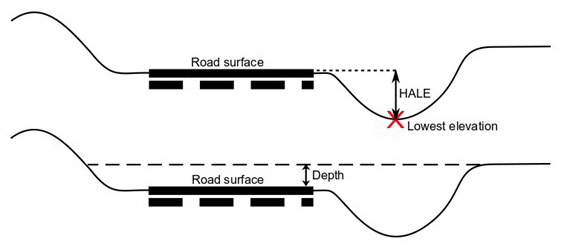
After delineating road surface depressions, physical descriptors of depressions and their upstream catchments are computed as follows. Two sets of characteristics, summarized in Table 1, are defined for every depression that is selected in the previous extraction step: physical depression descriptors (PDDs) and physical catchment descriptors (PCDs; Kalantari et al., 2014). PDD features describe the depression topography that is likely to affect water accumulation. These features are area, average depth assuming the depression is filled, and the height of road DEM cell elevations above the lowest elevation of the depression (hereafter called height above lowest elevation, or HALE). The HALE feature indicates which DEM cells on road surface would be inundated first and what is the accumulated depth required for flood water to reach that grid cell. Figure 3 shows a schematic of the HALE and depth features. The PCD features are derived from the upstream catchment that drains into each depression. The extracted features are average slope, fractions of the upstream catchment with a steep slope (defined as steeper than 8 %), percentage of imperviousness, and the net log-transformed drainage area, hereafter called net drainage area (NetDA), which is computed using Eq. (1):

$$\begin{array}{}\text{(1)}& \mathrm{NetDA}=\mathrm{Log}\left(\mathrm{CA}\right)\times I,\end{array}$$

where CA is the catchment area in m², and I is the percentage imperviousness of the catchment based on the National Land Cover Dataset (NLCD).

Log(CA) was used in this equation, reflecting the nonlinear relationship between catchment area and flood likelihood. This can happen since the larger the drainage area is, the higher are the impacts of infiltration, loss, and stormwater drainage that we are not considering in this analysis.

Table 1 Physical depression/catchment descriptors.

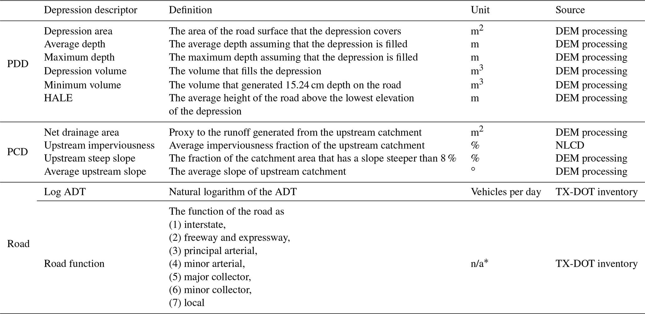
^* n/a: not applicable.

Figure 3 Schematic of HALE and depth features.

2.1.3 Traffic exposure

Crowdsourced data are generated by volunteer contributions, which results in more data availability on roads with higher traffic volumes. Therefore, including a feature in the model that captures roadway traffic exposure to flooded areas is necessary to consider the likelihood of reporting a flooded depression. For this purpose, two additional variables are included in the framework (Table 1): (1) the natural logarithm of annual daily traffic (ADT) and (2) the road function as defined by the Texas Department of Transportation (TX-DOT).

2.1.4 Storm event definition and storm clustering

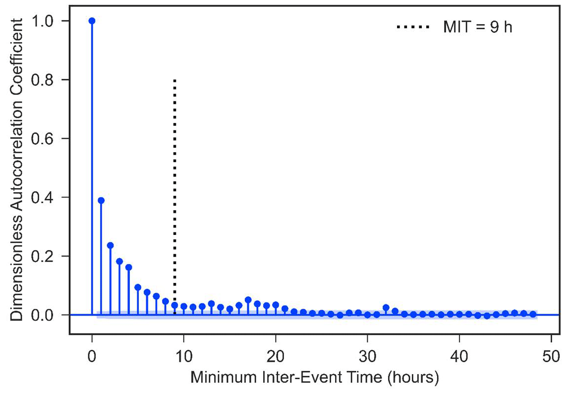
Raw precipitation data are obtained from Automated Surface Observing Systems (ASOS) stations in continuous 5 min interval rain pulse observations. To predict the probability of depression flooding during a storm of particular severity, independent storm events must be derived from the continuous data. In this study, the minimum inter-event time (MIT) method is used to define independent storm events. The MIT approach defines a storm event as rainfall that follows and is followed by a minimum dry (rainless) period called the minimum inter-event time. The MIT value can be calculated using different approaches. A reasonable estimate of the MIT value is the lag time at which the serial autocorrelation between rain pulses reaches a pre-set low threshold and remains steady (Asquith et al., 2005). In this study, the MIT value is diagnosed using the correlogram method to visualize the autocorrelation of a rain pulse time series to find the lag time that makes a rain pulse independent of its preceding rain pulses. After defining independent storm events, storm characteristics, including accumulated precipitation; duration; average intensity; and maximum 15 min, 30 min, and hourly intensities, are calculated.

In similar storm events characteristics, similar locations of depression PFF is likely to occur. To capture this phenomenon, storms are clustered into classes with similar severity (light, moderate, severe) using the storm characteristics such as intensity, rainfall depth, and storm duration. For storm clustering, agglomerative hierarchical clustering is applied using a bottom-up approach that forms a single cluster for each storm event and successively merges clusters based on Ward's linkage method. Ward's linkage method minimizes the total increase in within-cluster variance (Edelbrock, 1979) caused by merging clusters. The benefit of using agglomerative clustering is that this algorithm is less sensitive to outliers and avoids creating a large number of small clusters for extreme storm events (Edelbrock, 1979).

2.1.5 Waze data preprocessing

Waze is a GPS-based traffic navigation app that collects crowdsourced information about road conditions. The Waze app aggregates traffic incidents reported by its users as traffic alerts. Traffic alerts are geotagged points with two attributes that specify their lifetime: “publish date” and “last seen”. The Waze app has no pre-qualification for users to post a report, consequently not all of the flood-labeled alerts are reliable to be used as flood observations. Praharaj et al. (2021b) showed that 71 % of Waze flood alerts are reliable in Norfolk, Virginia. To investigate Waze alerts' authenticity, we matched flood-related alerts to the most recent rainfall event and computed the delay between alerts' publishing and rainfall end-time. A temporal threshold can be found by analyzing the cumulative distribution of delays that determines whether a flood report is related to a storm event.

In addition to alert timing, we also compared the locations of Waze alerts to publicly available datasets of high-flood-risk locations, including the National Flood Hazard Layer (NFHL), high watermarks and low water crossings data inventories from the North Central Texas Council of Government (NCTCOG), and the road surface depressions computed as described in the methodology section. The NFHL is a spatial dataset that uses river flood hazard information provided by the Federal Emergency Management Agency (FEMA) to generate flood hazard maps showing areas at high risk of flooding. We investigated the proximity of Waze alerts to the high-flood-risk locations to find the spatial accordance of flood alerts to these locations.

One challenge in adopting Waze flood-related alerts as roadway PFF observations is assigning the alerts to the appropriate flooded location because the coordinates of alert points do not perfectly align with flooded location coordinates. The distance between the flooded location and alerts depends on many unknown factors such as drivers' reaction times, direction, and sight distance. Posting a flood alert requires Waze users to complete three steps (three selections) in the app while driving or riding and users can post a flood alert before or after passing the flooded road segment. Hence assigning flood alerts to the proper depression must be done carefully. Waze data do not provide the direction of travel. However, no constraints regarding the travel direction have been used for assigning flood alerts to flooded depressions, since depressions can cross both sides of the road.

In this study, three independent individuals were each asked to separately visually assess a map of historical flood alerts laid over surface depressions and assign alerts to depressions using the following criteria: a cluster of more than two flood alerts should be available near the depression and the depression must be distinct from other nearby surface depressions. Flood alerts posted from bridges and elevated highways are excluded since BE-DEM does not represent bridge surfaces. Figure 4 shows a schematic example of alerts that can be assigned to the depicted depression and some that should remain unassigned because they are isolated and too far from a depression.

Figure 4 Alert assignment.

2.2 Step II: modeling

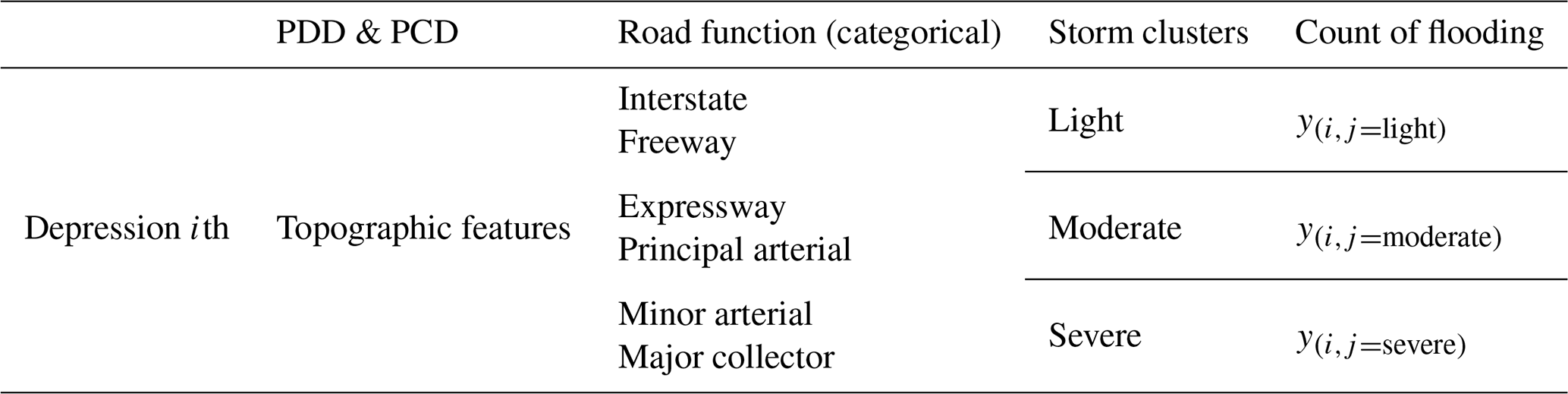
Pluvial flooding on any given surface depression is a binary variable that can be modeled as a Bernoulli trial of flood failure (i.e., non-flooded) or success (i.e., flooded). If a depression has one or more Waze flood alerts linked to it, the depression is labeled as flooded (success). Assuming that the probability of being flooded is smaller than the non-flooded situation and that the likelihood of flooding in a particular storm event for each depression only relies on its characteristics and the storm magnitude (i.e., is independent of the probability of flooding on other depressions), a random variable y_i,j will define the count of successes (flooding) out of the N trials (N storm events of cluster j) on depression i. The purpose of this study is to estimate the random variable y_i,j using extracted topographic features, road function, and storm severity. Both statistical and machine learning models are implemented to estimate y_i,j, namely empirical Bayes and random forest. Table 2 summarizes the categories of pre-processed independent variables used in the modeling.

Table 2 Count dataset of PFF events.

2.2.1 Empirical Bayes model

In a highly urbanized area there are numerous uncertain and unobserved site-specific features that affect localized PFF likelihood, such as storm inlet's age, capacity, and condition. For example, consider two road surface depressions (A and B) with similar PDD, PCD, road type, and ADT that experience the same storm. Suppose depression A is located in a neighborhood with lower infrastructure maintenance services, and its drainage system clogs more often. Then, despite similar descriptive features, higher flood frequency should be expected at depression A. The empirical Bayes (EB) algorithm, a simplified and faster version of Bayes theory, takes advantage of the historical count of reported flood events from the Waze data to better reflect the impacts of these types of uncertain and unobserved variables. The EB approach has previously been implemented in many fields to address the impacts of unobserved variables in estimating rare events, including hydrology. The EB method uses the joint global prior and site-specific counts and produces the posterior probability y_i by employing a weighted average as shown in Eq. (2) (Fill and Stedinger, 1998; Kuczera, 1982; Smith et al., 2014; Hauer et al., 2002; Lord et al., 2005; Strupczewski et al., 2001).

$$\begin{array}{}\text{(2)}& \mathrm{EB}\left(y\right)=w\times \mathit{\mu }+(\mathrm{1}-w)\times y,\end{array}$$

where w is the EB weight factor, μ is the expected flood frequency on depressions similar to a given depression, and y is the number of flood events on a given depression.

The expected flood frequency for similar depressions (μ) is the global prior probability distribution from a fitted regression model, which in this study is a negative binomial regression model. The number of flood events (y) is the historical site-specific flood event observation from the Waze data.

2.2.2 Negative binomial distribution

Based on Waze flood observations, the variance of flood frequencies on depressions with similar PDD, PCD, road type, and ADT is assumed to be greater than the average of flood frequencies (i.e., E(y)<Var(y)). This assumption is appropriate given the importance of unobserved variables on the PFF formation on roads such as storm inlet conditions. In other words, among n similar surface depressions, k depressions, where k≪n experience flooding significantly more than average. This fact leads to an over-dispersed dataset where E(y)<Var(y). Studies have shown that in the case of over-dispersed data, y_i follows a Poisson distribution with the rate parameter λ_i, where λ_i follows a Gamma distribution with the dispersion parameter ϕ and the rate parameter $\mathit{\varphi }/{\mathit{\mu }}_i$. The resulting distribution is Poisson–Gamma, also called the negative binomial (NB) distribution (Zou et al., 2017). The probability mass function of the NB distribution is given in Eqs. (3) and (4). Therefore, in this study, the expected flood frequency on similar depressions in the EB equation (Eq. 2) is derived from a negative binomial (NB) regression model that is fit to the count dataset shown in Table 2. NB parameters (ϕ and β_i) are estimated using the maximum likelihood estimation method.

$$\begin{array}{}\text{(3)}& P\left(y\right)={\displaystyle \frac{\mathrm{\Gamma }\left(y+\mathit{\varphi }\right)}{\mathrm{\Gamma }\left(y+\mathrm{1}\right)\mathrm{\Gamma }\left(\mathit{\varphi }\right)}}{\left({\displaystyle \frac{\mathit{\varphi }}{\mathit{\varphi }+\mathit{\mu }}}\right)}^{\mathit{\varphi }}{\left({\displaystyle \frac{\mathit{\mu }}{\mathit{\mu }+\mathit{\varphi }}}\right)}^y,\end{array}$$

where ϕ is the dispersion parameter of the NB distribution, y is number of flood events on depression i, and μ is the expected flood frequency on a given depression based on similar depressions (Eq. 4).

$$\begin{array}{}\text{(4)}& \mathit{\mu }=\exp \left(\sum {\mathit{\beta }}_k{x}_k\right),\end{array}$$

where β_k is the coefficient of kth regressor variable in the fitted regression model and x_k is the value of kth regressor on a given depression model selection for the NB regression model and is implemented using the Bayesian information criterion (BIC). In model selection, minimizing the BIC to the simplest model with the least number of exploratory variables is reasonable. Reducing the BIC by adding more explanatory variables increases the risk of overfitting and loss of generality. Equation (5) shows the calculation of BIC.

$$\begin{array}{}\text{(5)}& \mathrm{BIC}=-\mathrm{2}\log \mathrm{}\left(L\right)+K\cdot Ln\left(n\right)\end{array}$$

L is the maximum likelihood of the model representing the overall fit of the model, K is the number of model parameters, and n is the sample size.

It can be shown that the weight in the EB equation based on the NB regression is calculated as $\frac{\mathit{\varphi }}{\mathit{\mu }+\mathit{\varphi }}$; hence, we can rewrite Eq. (2) as Eq. (6). ϕ is the NB parameter (Eq. 3 estimated using maximum likelihood estimation). For more information regarding the mathematics of deriving the EB weight factor, refer to Zou et al. (2017).

$$\begin{array}{}\text{(6)}& \mathrm{EB}\left(y\right)={\displaystyle \frac{\mathit{\varphi }}{\mathit{\mu }+\mathit{\varphi }}}\mathit{\mu }+{\displaystyle \frac{\mathit{\mu }}{\mathit{\mu }+\mathit{\varphi }}}y,\end{array}$$

where ϕ is the dispersion parameter of NB distribution. The EB model's predictive power is estimated using the mean absolute error (MAE). The MAE shows the average error of the fitted values across the observations. The lower the MAE, the better the EB estimates fit the observations. The MAE is calculated using Eq. (7):

$$\begin{array}{}\text{(7)}& \mathrm{MAE}={\displaystyle \frac{\mathrm{1}}{n}}\sum _{i=\mathrm{1}}^n|y_i-{\widehat{y}}_i|,\end{array}$$

where n is the sample size, y_i is number of flood events on depression i, and ${\widehat{y}}_i$ is the EB predicted number of flood events on depression i.

2.2.3 Random forest

Random forest (RF) is a supervised ensemble machine learning algorithm that uses multiple decision tree learners to increase predictive performance (Breiman, 2001). A decision tree consists of a hierarchy of nodes, each of which represents a conditional decision rule that splits the data into different decision paths. The final prediction of RF is the average prediction of all decision trees; each tree is built from a bootstrap sample of observations and a subset of features. The RF has been widely used for data-driven modeling in the field of water resources (Sadler et al., 2018). This algorithm can handle large and imbalanced datasets and is well known to be easy to train. An important strength of the RF is that its convergence rate is independent of noise and sparsity in the descriptive variables. RF models are useful for estimating the contribution of features in the target variable (in this case, flood frequency). The node impurity in each node of the RF is the measure of homogeneity of the target values at that node, which is the variance of target values in a regression problem. The normalized reduction in the node impurity achieved by adding a specific feature to a tree defines the importance of that feature. In RF, the average of importance of a feature in all trees weighted by the number of samples involved in each split is the overall feature importance.

In this study, RF regression is executed using the Scikit-Learn library in the Python environment (Pedregosa et al., 2011). The number of decision tree learners in the RF regression is optimized by the algorithm. For hyperparameter tuning and model selection, a randomized cross-validated grid search is applied on a wide range of model parameters and MAE is used to measure parameter performance and select the best-performing parameter set. The resulting parameters are then used to estimate the frequency of PFF at every depression for each storm class using Eq. (8).

$$\begin{array}{}\text{(8)}& \mathrm{RF}\left(y\right)=\mathrm{RF}(\mathrm{PDD},\mathrm{PCD},\mathrm{road}\mathrm{features},\mathrm{storm}\mathrm{type}),\end{array}$$

where RF(y) is the random forest prediction of number of flood events on a given depression.

2.2.4 Model evaluation

To evaluate the performance of the proposed model, the following approaches are used. First, 80 % of the historical data, randomly selected, are used in model training. Model testing is then implemented using the remaining 20 % of the data held out from the training process. The performance of the models is then assessed using the MAE of the predictions. In order to ensure that the models are stable and their performance does not change with different train-test sets, the models are trained and evaluated for several randomly chosen training sets and the variation in their performance is considered in selecting the best models for the final step of the framework.

Then, to further assess the improvements in PFF event estimation using topographic and historical Waze observations, the EB and RF models are compared with three simple benchmark models. First, the average model (Eq. 9) assumes that the average PFF counts from historical Waze observations apply to all depressions and all storms without considering storm type and topographic feature. Second, the storm-based average model uses the average of the PFF count in each storm cluster without considering topographic features (Eq. 10). Finally, a regression model is used that predicts PFF based on topographic, road type, and storm features but without implementing EB to update the prior probability (Eq. 4).

$$\begin{array}{}\text{(9)}& p_i=\sum _{i=\mathrm{1}}^n{\displaystyle \frac{y_i}{N_{\mathrm{t}}}},\end{array}$$

where p_i is the likelihood of flooding on depression i, y_i is the number of reported floodings on depression i, n is total number of depressions, and N_t is number of total storm events.

$$\begin{array}{}\text{(10)}& p_{i,j}=\sum _{i=\mathrm{1}}^n{\displaystyle \frac{y_{i,j}}{N_j}},\end{array}$$

where p_i,j is the likelihood of flooding on depression i and storm type j, y_i,j is the number of reported floodings on depression i and storm type j, and N_j number of total storms of cluster j.

2.3 Step III: flood probability estimation

Finally, in Step III, the most accurate model from Step II is used to produce flood probability maps for every storm cluster across the region of interest. The probability of flooding is calculated using Eq. (11).

$$\begin{array}{}\text{(11)}& p_{i,j}={\displaystyle \frac{{\widehat{y}}_{i,j}}{N_j}},\end{array}$$

where ${\widehat{y}}_{i,j}$ is the predicted number of floodings on depression i and storm type of j.

3 Case study background and datasets

The described methodology was evaluated in the city of Dallas, Texas, USA (Fig. 5), which is the third-largest city in Texas with a population of more than 1 million. Dallas' elevation ranges from 137 to 168 meters (450 to 550 ft), and it is mostly flat. According to the Texas Department of Transportation (TXDOT), almost 20 % of crashes, equal to 248 vehicle crashes in the City of Dallas in 2018, happened on either standing water or wet road surface conditions. According to an analysis conducted by the First Street Foundation, flooding can expose 1841 mi of Dallas roadways (out of 6064 mi) to the risk of becoming impassable (F. S. Foundation, 2020). However, currently available fire-rescue dispatch software, including that used by the Dallas Fire Rescue Department (DFRD), assumes empty and dry roads for routing rescue vehicles. This has resulted in rescue delays and occasional loss of life on flooded roadways, which provided the motivation for this study.

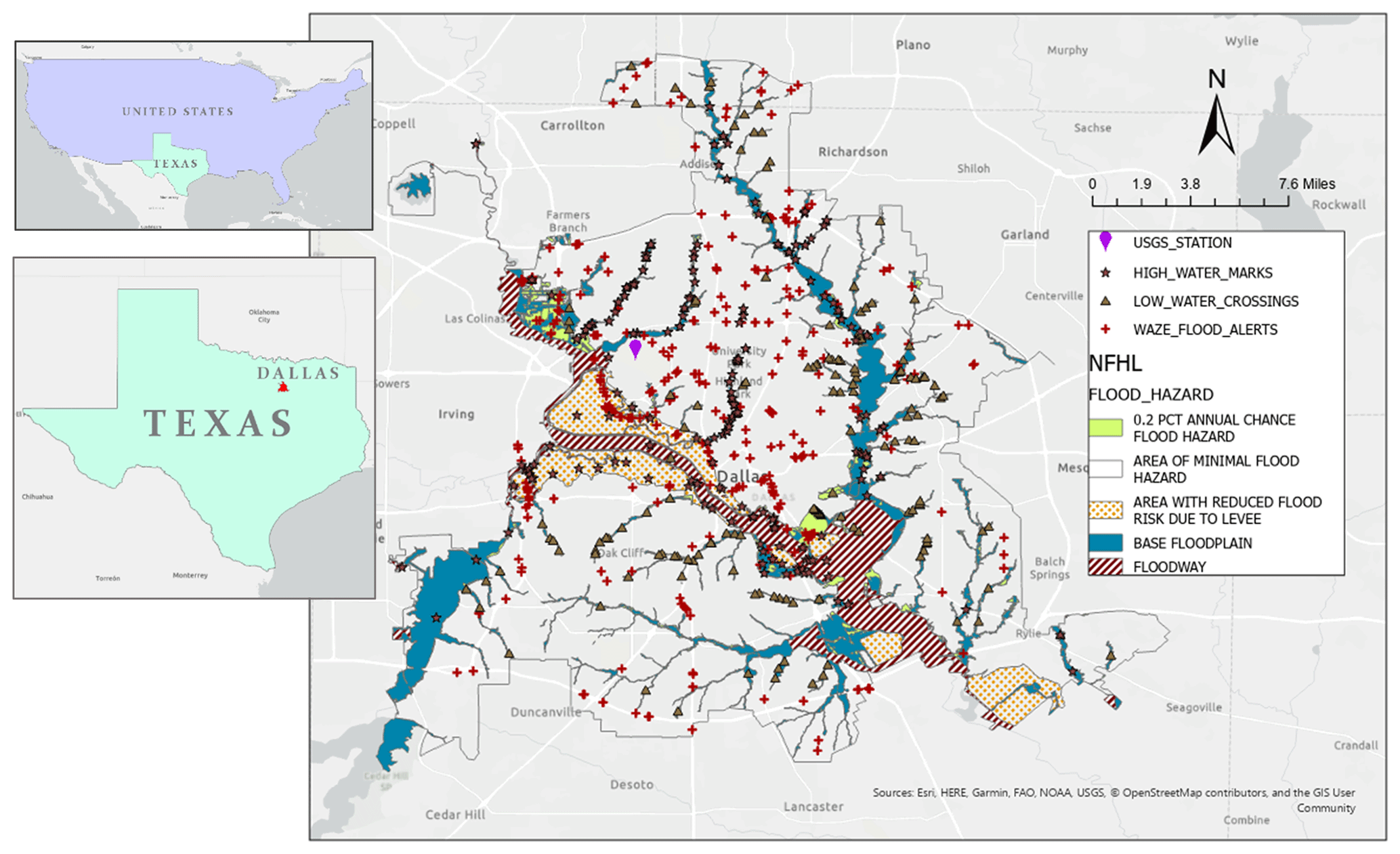
Figure 5 Study area and datasets (basemap from ESRI-2021).

For this case study, several datasets were used. First, a 1 m resolution bare-earth digital elevation model (BE-DEM) was obtained from the North Central Texas Council of Government (NCTCOG), which was derived from a quality level 2 Lidar survey performed by Digital Aerial Solutions, LLC, in 2018, under contract with the Unites States Geological Survey (USGS) and National Resources Conservation Services (NRCS). The BE-DEM dataset's name is TX Pecos Dallas 2018 D19, with horizontal accuracy of ±0.682 m at a 95 % confidence level and non-vegetated vertical accuracy (NVA) of 0.196 m.

For rainfall, 15 min precipitation observations were obtained from the USGS ASOS station at Dallas Love Field Airport (DAL; Fig. 5). Precipitation observations from 1 January 2017 to 1 March 2020 were used. Next, the US Department of Agriculture's (USDA) National Land Cover Database (2016; Homer and Fry, 2012) is used to extract catchment imperviousness. The imperviousness raster over Dallas has a 30 m resolution and ranges from 0 % to 100 %, with a mean of 33.87 % and standard deviation of 32.98 %.

Waze alerts were obtained from the NCTCOG, which is a Waze partner in the Waze Connected Citizen Program (CCP). The NCTCOG granted us access to the Waze data for the period of 21 April 2018 (the start of NCTCOG's Waze partnership) to 20 March 2020. Waze alerts are classified into seven main categories: accident, jam, construction, miscellaneous, hazard or weather (hazard-weather), road-closure, and others. The “hazard-weather” data itself are divided into several subcategories. Alerts in the “flood” subcategory and ones which have any form of the word “flood” in their report description, such as “right lane flooded”, are potentially flood-related and were included in this study, resulting in 5652 Waze alerts.

The locations of these Waze alerts were shown in Fig. 5, along with the NFHL river flood zones. Figure 6a shows that the majority (around 70 %) of alerts during the study period were posted in areas with minimal river flood hazard, which comprise approximately 76 % of the study area (Fig. 6b). Another 18 % of the alerts were posted in areas of reduced river flood risk due to levees, which were not breached during the study period. This indicates that PFF is likely the cause of most Waze alerts.

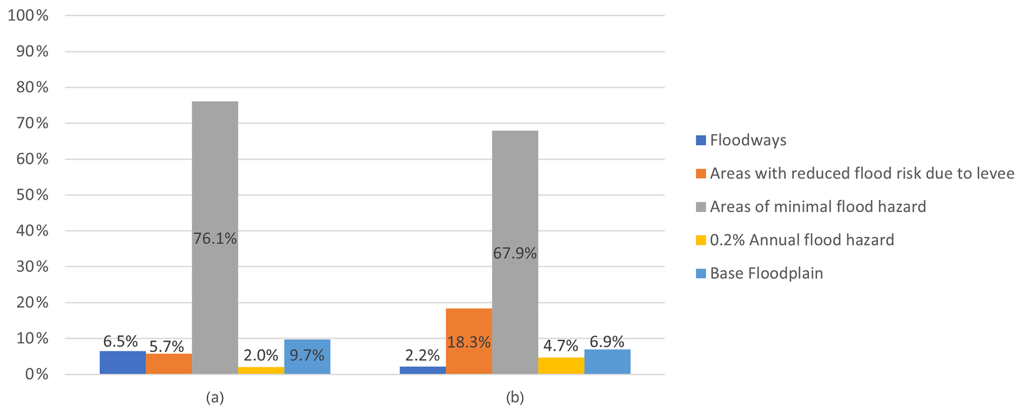
Figure 6 (a) Distribution of NFHL flood zone areas across the study region, (b) flood alerts in NFHL flood zones.

To further investigate the potential causes of Waze flood alerts, the high-water marks inventory and low-water crossing dataset were obtained from the Texas Natural Resources Information System (TNRIS). The high-water marks inventory contains historic high water level reports from flooded water bodies or structures at 334 locations across the city of Dallas (Fig. 5). The low-water crossing dataset includes 175 locations where surface water has crossed roads during high-flow conditions (Fig. 5). Analyzing Waze alert distances to the nearest high-water mark and low-water crossing shows that the vast majority of alerts are more than 200 m from both low-water crossings and high-water marks (Fig. 7).

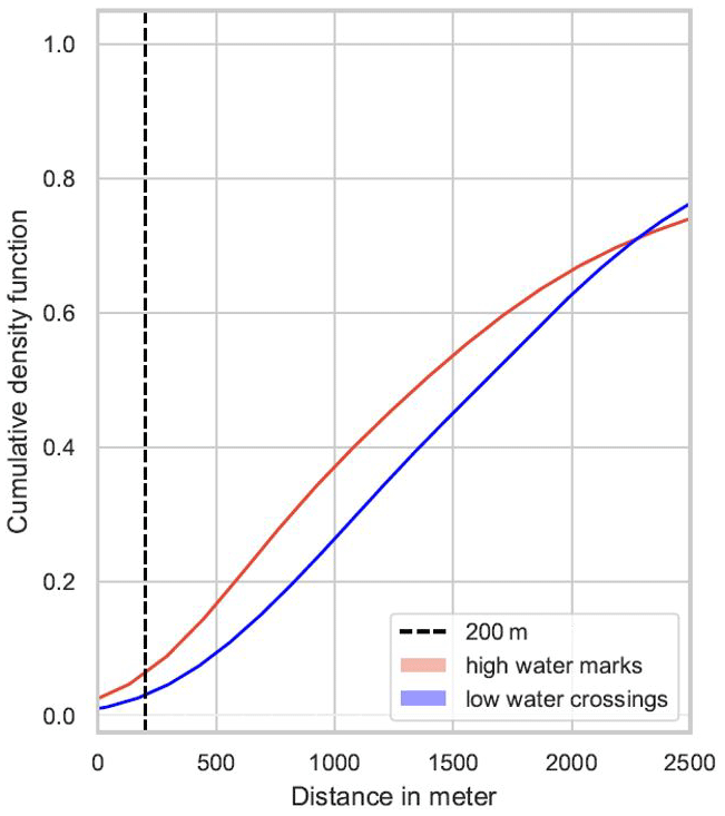
Figure 7 Cumulative density of alert distances to the closest high-water mark and low-water crossing.

These findings show how complementary flood observations such as Waze data are needed to assess roadway conditions more comprehensively than available official datasets. Thus, in order to predict local roadway PFF, it is necessary to consider local surface depressions as low-lying areas where surface runoff can accumulate during storms.

4 Data pre-processing results

4.1 Depression extraction

Following the procedure explained in the methodology, almost 380 000 surface depressions were extracted over the city of Dallas. Only 315 depressions are located on roads and are deeper than 6 in. Among these 315 depressions, 191 depressions were proximal to reliable Waze flood alerts more than twice. To consider only chronically flooding areas, the rest of this analysis is focused only on these 191 surface depressions.

4.2 Storm event definition

As can be seen in Fig. 8, the autocorrelation coefficient of rain pulses first reaches a low value and remains steady at a lag time of 9 h; accordingly, MIT =9 h is chosen to convert the continuous precipitation data into independent storm events.

Figure 8 Autocorrelation of rain pulses.

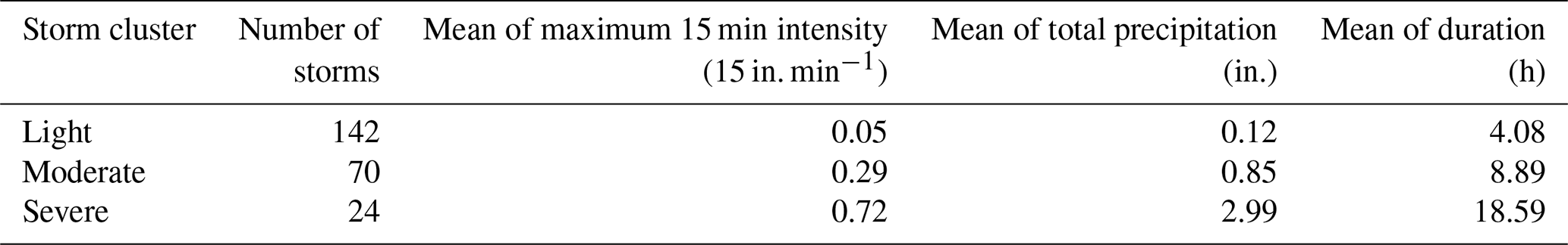
Using MIT =9 h, 236 independent storm events are extracted from 1 January 2017 to 1 March 2020. Storm characteristics are then tested for their utility in generating independent storm clusters with comparable storms. The maximum 15 min interval intensity and the total accumulated precipitation were found to generate the most comparable storms with agglomerative clustering. Figure 9 shows the dendrogram that illustrates how clustering the storms into three groups captures acceptable dissimilarity between storm severity, which are defined as light, moderate, and severe storms. The vertical axis of the dendrogram depicts the dissimilarity between storms, and the horizontal axis represents storms. The position of each split on the vertical axis shows the dissimilarity of the two clusters on sides of the split. Table 3 shows summary statistics for the three storm clusters.

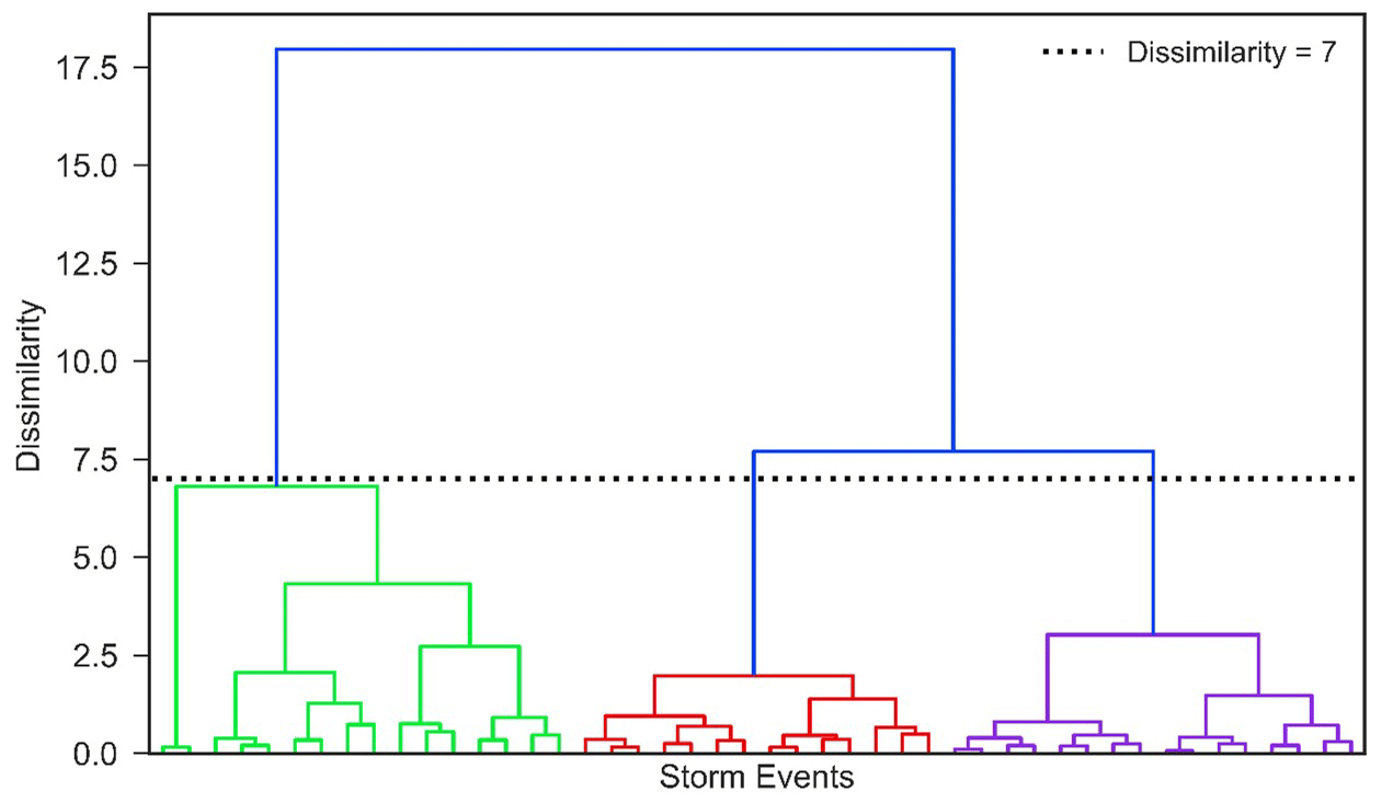
Figure 9 Tree-based dendrogram of agglomerative clustering; green, red, and purple lines represent within-cluster dissimilarities in light, moderate, and severe storms, respectively.

Table 3 Summary statistics of storm clusters.

4.3 Waze data preprocessing

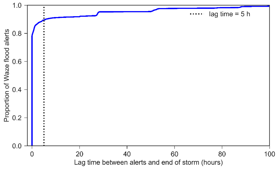
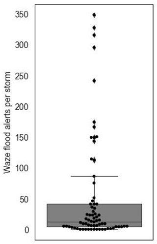
Potential flood-related alerts posted in the time span of 21 April 2018 to 20 March 2020 are matched to their preceding storm. Figure 10 gives the distribution of delays between the alert's published time and storm end. Figure 10 shows that more than 90 % of Waze flood alerts are posted within 5 h of storms. Therefore, potential flood-related alerts posted later than 5 h after storms were considered outliers (noise) and removed from the analysis. This process left 4996 flood-related alerts out of the initial 5652 alerts. The number of flood alerts posted per storm event ranged from 0 to 375, with the distribution depicted in Fig. 11. During the study period, 150 storms occurred but only 98 storms caused Waze flood alerts. On average, each storm event had 10 flood alerts. The process of flood alert assignment explained in the methodology section was performed for the 4996 flood alerts in the Dallas case study by three independent individuals. With the given criteria, where more than four alerts were clustered around a depression, 100 % agreement between the annotators was observed in the assignment of alerts to depressions. Disagreement between annotators in alert to depression assignment was observed in locations where less than four alerts are clustered around a depression. The first author reviewed alerts that indicated disagreement, and if the specified criteria for making the assignment were not met, alerts were removed from the analysis. Among the 4996 flood alerts that were filtered, 2665 alerts were assigned to 191 independent surface depressions using the approach described in the methodology section (Sect. 2.1.5).

Figure 10 Distribution of delay in alert posting from storm end.

Figure 11 Total number of flood-related alerts per storm.

5 Modeling results

The performance of the proposed framework in estimating flood frequency is evaluated using both the empirical Bayes (EB) and random forest (RF) models and compared to the baseline models. Results from the best-performing model, EB, are then examined in more detail in the following sections.

Table 4 NB model estimation results.

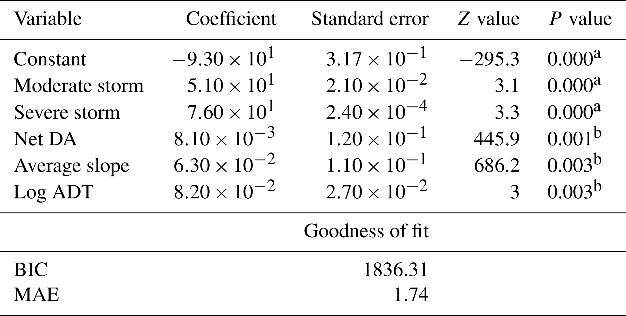
^a Significant with more than 99 % confidence. ^b Significant with more than 95 % confidence.

Figure 12 Prediction of the number of roadway PFF events.

5.1 Model parameters and performance

Parameters for the fitted NB model (Eq. 4) are presented in Table 4. The dispersion parameter of the fitted NB regression model (ϕ of Eq. 3) is 2.943. A value of ϕ>1 demonstrates that the over-dispersion assumption is valid, whereas ϕ<1 shows an under-dispersed dataset. The MAE value achieved from fitting the NB distribution is 1.74, which shows that the flood frequencies fit to the prior probability distribution have an average error equal to 1.74 flood events out of 150 storms. The EB estimate of the fitted NB regression model, computed based on Eq. 6, reduces the MAE on the training set to 0.88 flood events.

Figure 13 Prediction of the number of PFF using benchmark models and EB.

For the RF model, hyperparameter tuning is implemented using a 3-fold cross-validated randomized search in the Scikit-Learn library in Python programming environment. The best-performing model is found to have 10 trees. The features with the highest importance (based on impurity-based feature importance calculated by the Scikit-Learn library) in the RF model are severe storms, maximum depth, average upstream slope, log ADT, and the net drainage area. The MAE of RF estimates on the training set is 0.73.

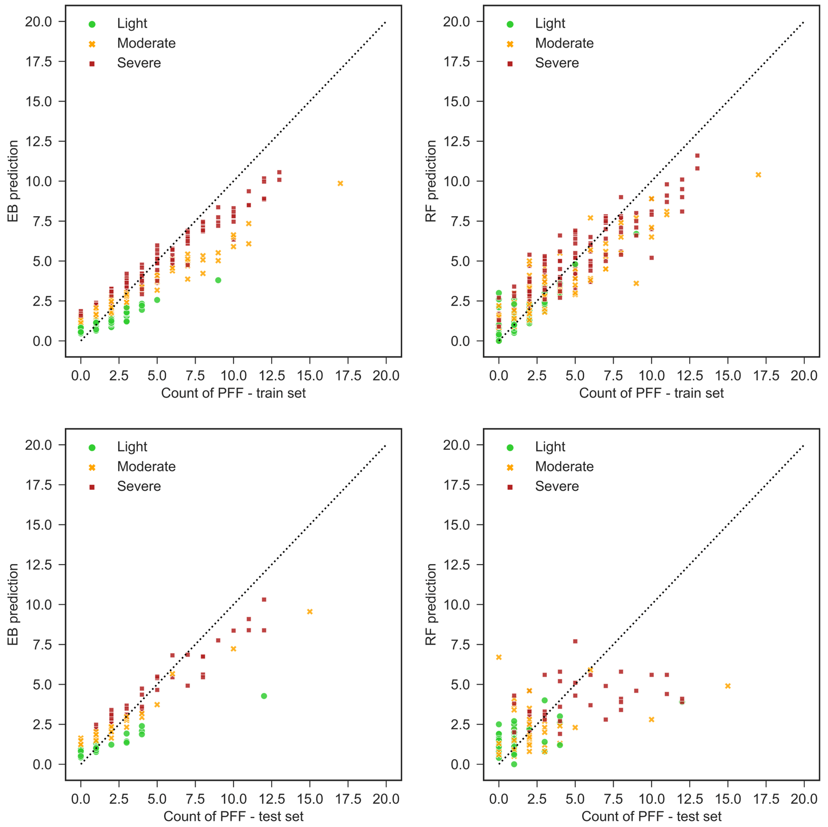
The predictive power of both models is evaluated on the held-out test dataset. The EB approach predicts the number of flood events for unseen situations with MAE =0.92, while the RF model's evaluation MAE is considerably higher, with MAE =2.1. To minimize the impact of particular train-test datasets on the model's performance, the dataset is randomly split 50 times and the model performance statistics are re-evaluated for each split. The EB model has an average MAE of 0.89, as opposed to the average MAE of 1.92 attained by the RF model. EB's predictive capability is also more stable across the 50 runs than the RF model, with the standard deviation of MAEs attained from different runs being 0.11 and 0.18, respectively. Figure 12 shows the prediction power of the models on the train and test datasets.

It can be seen that the RF model is a better fit on the training dataset, but its lower performance on the test set shows that it is overfitting on the training set while the EB approach has more consistent performance on both datasets. The superiority of the EB model shows that the unobserved features play a significant role in PFF formation on road segments and a Bayesian approach is more successful in capturing the effects of these features.

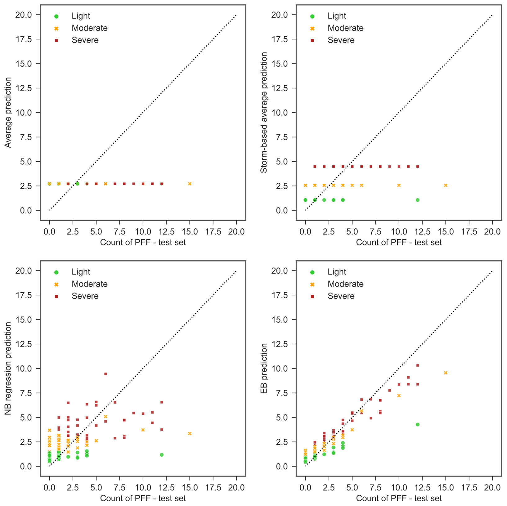
Next, the EB model that is found superior to the RF model is compared with the simple benchmark models given in the methodology section. Figure 13 demonstrates how the flood counts will be predicted on the test dataset using each benchmark model, NB regression, and EB model. Table 5 summarizes the performance of the EB approach, NB regression, and benchmark models. It can be seen that the MAE for both training and testing sets improves by adding storm clusters to the average model. This increase is more noticeable in light storms (almost 50 % improvement for both training and testing dataset).

Table 5 Summary performance of models.

However, adding topographic and observed flooding variables, as in the EB model, increases the accuracy of PFF count estimation for severe storms more than moderate and light storms. This shows that topographic features are more important in the formation of PFF when storms are more severe. Also, if PFF is observed at a particular location, then it is more likely to be observed at that depression again.

5.2 Flood likelihood estimation

The EB approach is superior in predicting the total number of flood events; hence, this approach is used to estimate flood likelihoods from the frequency of PFF events (Eq. 11). Figure 14 shows a higher PFF likelihood during severe storms compared to light and moderate storms. Generally, we can see that flood likelihoods are higher when flooding has been posted. However, as discussed in the methodology section, true negative situations cannot be identified with voluntary crowdsourced data (i.e., there could be flooding that no Waze user has reported).

Figure 14 Distribution of flood likelihoods in reported versus non-reported floods.

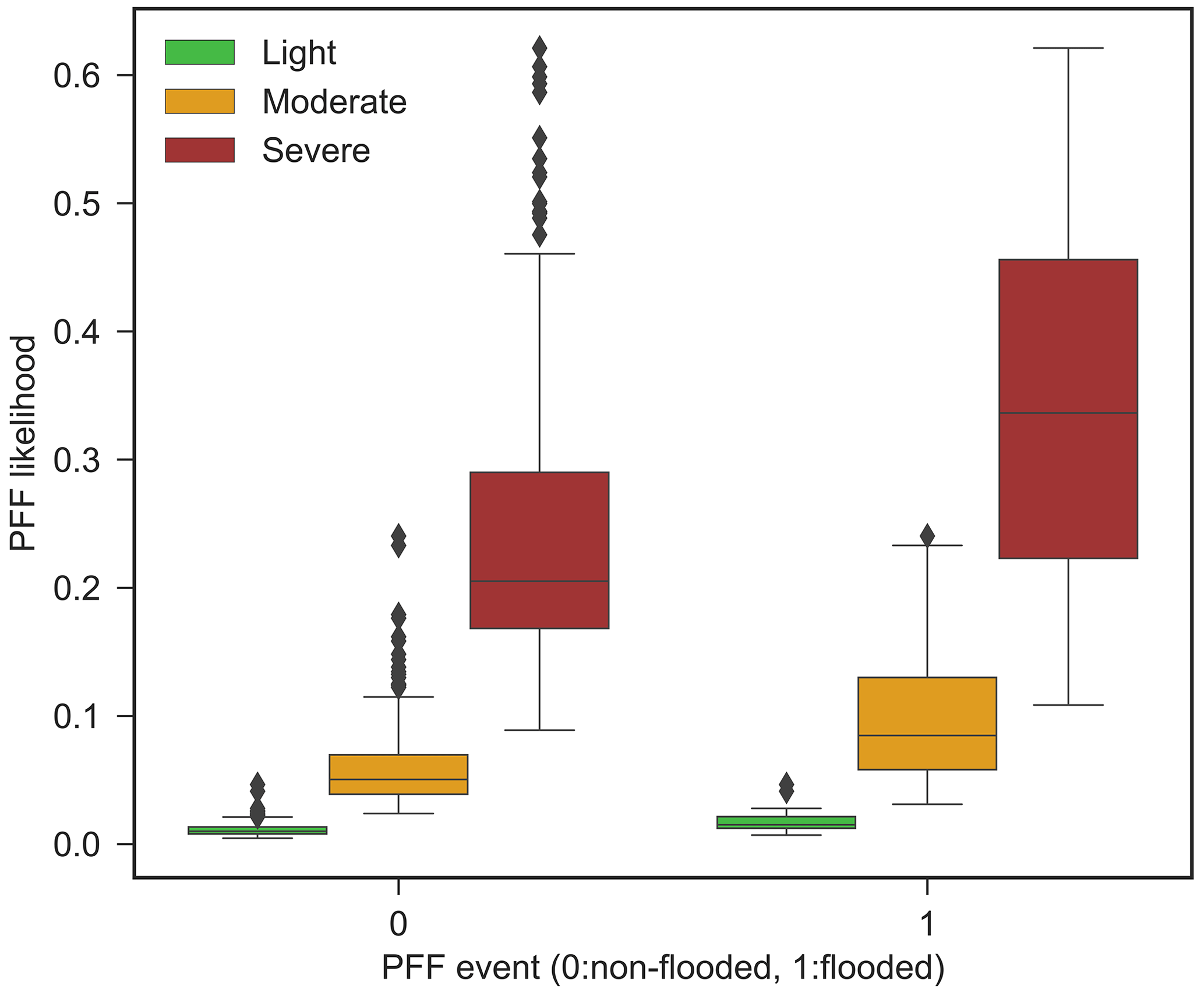
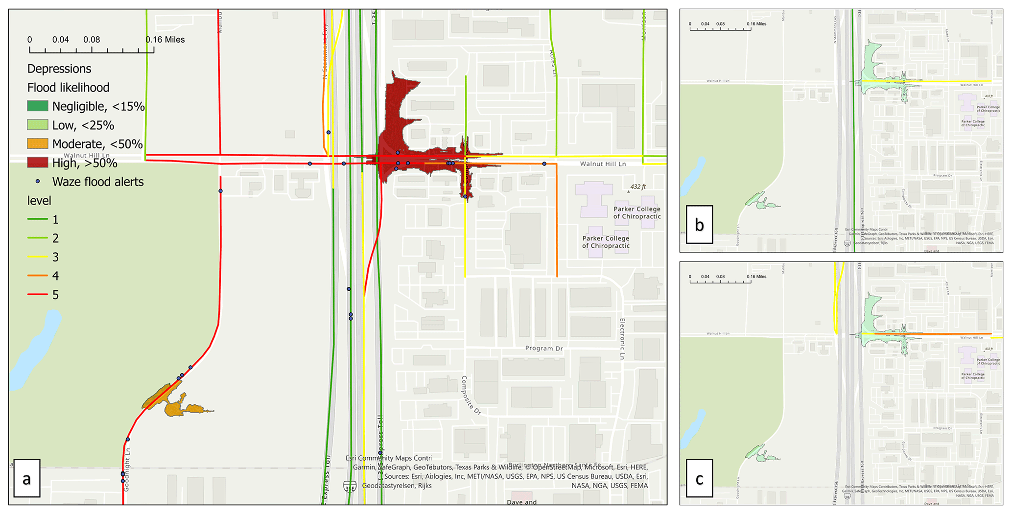
Figure 15 PFF probability map versus flood alerts and traffic jams from 13:00 to 17:00 CST on (a) Friday, 22 September with a severe storm; (b) Friday, 29 September 2018, rainless; and (c) Friday, 15 September 2018, rainless.

Figure 14a shows an example of a flood probability map for severe storms, along with historical flood-related alerts and traffic jams reported by Waze during one particular severe storm that occurred on 22 September 2018. Figures 14b and c show the same information during the same time and day of the week for the following and preceding weeks. Waze traffic jam reports include severity and congestion levels ranging from 1 (lowest) to 5 (highest), which denote the level of traffic slow down or complete shutdown. Negligible, low, moderate, and high flood probabilities are defined as less than 10 %, less than 30 %, less than 50 %, and higher than 50 %, respectively. In Figure 14a, high traffic levels (Waze jam levels of 5) can be seen near a depression with high PFF probability (more than 50 %). Figure 14 indicates that traffic jams during severe storm are noticeably higher than at similar time intervals before and after the storm. These maps suggest that the traffic jam on the storm date, which agrees with the flood likelihood, is likely to be an anomaly relative to typical traffic conditions at this intersection. This finding is consistent with the flood alerts and predictions of severe flooding at this location during the storm.

6 Discussion

The EB model is superior compared to the RF and benchmark models in predicting the number of flood events; hence, this model is used to estimate flood probabilities for storm clusters. The distribution of estimated flood probabilities (Fig. 14 and Table 5) are plausible given the magnitude of the storms. For example, the light storms have an average duration of 4 h and an average total precipitation of 0.1 in., which is quite low and flooding would not be expected during these storms. Flood-related alerts that are posted during these rainfall events can be assumed to be noise and disregarded for future studies. Based on the NB regression line that is fitted to the count of observed flood events, we expect to see 7.6 and 5.2 times more flood events in moderate and severe storms, respectively, compared to light storms. The NB model also shows that increases in the upstream net drainage area and average slope increase the probability of flooding, as would be expected. Furthermore, log ADT has a direct relationship with the probability of observing a PFF event because frequently traveled roads are more likely to have Waze postings. This finding shows the limitations of estimating flood events from crowdsourced Waze datasets that tend to neglect flood events on less-traveled roads. The superior performance of the EB approach shows the significant impact of unobserved site-specific features such as stormwater inlet conditions in predicting the likelihood of PFFs on roadways. By using historical observations, the EB approach better identified frequently flooded locations (road surface depressions), perhaps due to site-specific features such as under-sized stormwater inlets. Data were not available on these features for this study. In highly urbanized areas, these types of uncertainties in engineered structures, particularly in older areas of the city where record keeping can be poor, add to temporal uncertainties such as changing climate and land use that can affect flood formation. Despite these limitations, this study showed that localized traffic-related flood alerts are helpful in estimating PFF probabilities over a 3-year period. For longer periods, periodically retraining the model to account for changes in infrastructure and climate is recommended.

To make effective use of crowdsourced traffic data, extensive preprocessing is needed to evaluate the reliability of the data and map flood alerts, which are not necessarily posted at the exact location of the flooding, to plausible nearby depressions. This process, which was done manually in this study, can introduce errors and bias to the analysis. With more data and integration of other data sources (e.g., flood sensors and stormwater inlets), an automated mapping process could be developed that could potentially reduce these errors.

Furthermore, the approach taken in this study only considers flood-prone locations reported by Waze users. Numerous parameters affect human exposure to flooded locations, such as the number of Waze users that pass a road segment, road type, road function, day of week, and time of day. Hence, a similar flood extent on the road can cause significantly different magnitudes of traffic disruption at different times and locations and, therefore, different flood reports. Data-driven models also have limitations due to the previously discussed dataset constraints.

The EB model accounts for heterogeneity by utilizing historical frequencies. However, because of the bias and uncertainty in the Waze data, as discussed in Sect. 2.1.5, the EB model estimates will be skewed and less accurate for depressions situated on local and less-traveled routes. While major routes are more important than minor routes for minimizing exposure to roadway PFF, these limitations must be acknowledged. It is possible that, with more data, an approach to extrapolating findings on major roads to minor roads could be developed. To develop a more unbiased flood prediction model, we suggest that crowdsourced data be used as complementary data in conjunction with other data sources and models to account for less frequently traveled areas and times (e.g., during the Covid-19 pandemic, which was not included in this study, when traffic was significantly reduced).

7 Conclusions

This analysis is a first step in exploring approaches to implement crowdsourced data from the Waze app into flash-flood prediction. For this case study, Waze flood alerts were primarily posted in areas outside of mapped river flood hazards and low water crossings, suggesting the need for and importance of modeling rainfall-induced or pluvial flash flooding (PFF). The statistical and machine learning (ML) models implemented in this study demonstrated the feasibility of modeling PFF in terrain depressions based on storm, catchment, and road properties. The EB approach is found to be superior in terms of predictive power compared to RF. This shows the importance of unobserved site-specific features on roadway PFF, which the EB approach captures by incorporating historical site-specific PFF observations to produce posterior probability. Both statistical and machine learning models achieve smaller MAEs for severe storms compared with moderate and light storms. This shows that the modeled depression and catchment descriptors are more explanatory in severe storms when infiltration is reduced and drainage systems are more likely to be overwhelmed. The high accuracy of the proposed methodology in the Dallas case study shows that crowdsourced traffic data have value for high spatiotemporal resolution flash flood prediction. Stakeholders and decision-makers could benefit from the developed model for identifying locations that require stormwater utility maintenance or capital investment. Further research is needed to fully exploit crowdsourced data applicability as a complementary data source using more authoritative data sources and physics-based models.