Generating landslide density heatmaps for rapid detection using open-access satellite radar data in Google Earth Engine

Rapid detection of landslides is critical for emergency response, disaster mitigation, and improving our understanding of landslide dynamics. Satellite-based synthetic aperture radar (SAR) can be used to detect landslides, often within days of a triggering event, because it penetrates clouds, operates day and night, and is regularly acquired worldwide. Here we present a SAR backscatter change approach in the cloud-based Google Earth Engine (GEE) that uses multi-temporal stacks of freely available data from the Copernicus Sentinel-1 satellites to generate landslide density heatmaps for rapid detection. We test our GEE-based approach on multiple recent rainfall- and earthquake-triggered landslide events. Our ability to detect surface change from landslides generally improves with the total number of SAR images acquired before and after a landslide event, by combining data from both ascending and descending satellite acquisition geometries and applying topographic masks to remove flat areas unlikely to experience landslides. Importantly, our GEE approach does not require downloading a large volume of data to a local system or specialized processing software, which allows the broader hazard and landslide community to utilize and advance these state-of-the-art remote sensing data for improved situational awareness of landslide hazards.

1 Introduction

Rapid response to landslide events (and other natural hazards) is necessary to assess damage and save lives. This response effort includes ground-based teams of local residents, government officials and logistics coordinators, scientists, engineers, and more, all working together to identify critically damaged areas (e.g., Benz and Blum, 2019; Inter-Agency Standing Committee, 2015). Yet, many response efforts are impeded by a lack of detailed information on the condition or location of damaged areas following large and widespread landslide events (Lacroix et al., 2018; Robinson et al., 2019). In addition to rapid response efforts, it is also important to construct accurate landslide inventories in the weeks to months following these events (Froude and Petley, 2018; Roback et al., 2018; Williams et al., 2018). These detailed inventories are used to improve understanding of where landslides occur; to quantify erosion; and to look for areas where secondary hazards, such as outburst flooding due to landslide dams, may be occurring (Collins and Jibson, 2015; Kirschbaum et al., 2015; Kirschbaum and Stanley, 2018; Roback et al., 2018). It is therefore necessary to develop tools with freely available data that can be used to map the landslide extent and level of damage following catastrophic events.

Remote sensing techniques are commonly used to construct landslide inventories over large areas following catastrophic events (e.g., Bessette-Kirton et al., 2019; Roback et al., 2018). Satellite-based optical imagery provides high-quality information for landslide mapping. Many studies have leveraged these data with manual (e.g., Harp and Jibson, 1996; Massey et al., 2020) and semi-automated and/or automated mapping techniques to identify landslides (e.g., Amatya et al., 2019, 2021; Ghorbanzadeh et al., 2019; Hölbling et al., 2015; Lu et al., 2019; Mondini et al., 2011, 2013; Stumpf and Kerle, 2011). While optical imagery provides high-quality data, it is often limited in rapid response efforts because optical imagery requires daylight as well as shadow- and cloud-free conditions for accurately identifying landslides. Persistent cloud cover can prevent landslide mapping from satellite optical imagery for weeks to months (e.g., Lacroix et al., 2018; Robinson et al., 2019).

Satellite-based synthetic aperture radar (SAR) circumvents some of the optical data limitations because it can penetrate clouds and operate day or night, but SAR data are still limited by geometric shadow and distortion (e.g., Adriano et al., 2020; Mondini et al., 2021). SAR data have been used for nearly 2 decades to investigate landslides (e.g., Colesanti and Wasowski, 2006; Hilley et al., 2004; Roering et al., 2009). However, most studies have focused on interferometric SAR (InSAR), which measures the radar phase change between two acquisitions in order to quantify ground surface deformation (e.g., Handwerger et al., 2019; Huang et al., 2017b; Intrieri et al., 2017; Schlögel et al., 2015).

SAR backscatter intensity- and coherence-based change detection can also be used to detect landslides, floods, and other types of natural hazards (Burrows et al., 2020; DeVries et al., 2020; Jung and Yun, 2020; Mondini et al., 2019, 2021; Rignot and Van Zyl, 1993; Tay et al., 2020; Yun et al., 2015). Changes in backscatter and coherence occur when there are changes in ground surface properties (e.g., reflectance, roughness, dielectric properties) before and after landslide events. Coherence-based change detection methods work best in urban areas because normally the coherence is high prior to an event and there is a reduction in coherence from damage after an event. However, backscatter change detection methods can outperform coherence-based methods in densely vegetated mountainous regions because in these areas coherence is always low (i.e., no change) while the backscatter can change (see Jung and Yun, 2020, for a detailed comparison between these methods). Currently, SAR-based change detection methods are under-utilized for landslide identification following catastrophic events, which we believe is primarily due to data access and the specialized processing and software required to analyze SAR data.

In this study, we develop tools and strategies to detect individual landslides and areas with high landslide density (i.e., heatmaps) that can aid in rapid response and in constructing landslide inventories. We define rapid response landslide detection as the period of time within 2 weeks of a landslide event (Burrows et al., 2020; Inter-Agency Standing Committee, 2015; Williams et al., 2018). Our tools run in Google Earth Engine (GEE), a free cloud-based online platform, using only freely available data (Gorelick et al., 2017). Recent studies have used GEE to identify floods (e.g., DeVries et al., 2020) and landslides (e.g., Scheip and Wegmann, 2021), investigate land cover (e.g., Huang et al., 2017a) and surface water change (e.g., Donchyts et al., 2016), monitor agriculture (e.g., Dong et al., 2016), and more. For landslide detection, we measure changes in SAR backscatter from the open-access Copernicus Sentinel-1 (S1) satellites. Our approach requires the spatial coordinates of the area of interest (AOI) and the dates and duration of the landslide-triggering event. We test our landslide detection tools for recent events occurring under different environmental conditions. To better investigate landslide detection for different types and sizes of landslide, we analyze (1) the 2018 rainfall-induced landslides in Hiroshima Prefecture, Japan; (2) the 2018 earthquake-triggered landslides in Hokkaidō, Japan; (3) 2020 rainfall-triggered landslides in Huong Phung, Vietnam; and (4) 2020 rainfall-triggered landslides in Quang Nam, Vietnam (Fig. 1). To determine the most effective strategies for landslide detection, we perform a sensitivity analysis for the 2018 Hiroshima event by varying the time span (i.e., number of images) of SAR data used to measure changes in backscatter before and after the landslide-triggering event and by incorporating topographic slope- and curvature-based masks to remove regions where landslides are unlikely to occur. We then apply our most effective landslide detection strategies to the other case studies. We do not make systematic quantitative comparisons with other remote-sensing-based data used for landslide detection – e.g., SAR-based coherence (data not available in GEE) or the normalized difference vegetation index (NDVI). However, we do make quantitative comparisons of our findings with optical-data-based landslide inventories and qualitative comparisons with optical data from the Copernicus Sentinel-2 (S2) satellites for validation of our SAR-based landslide detection. Lastly, we applied our landslide detection tools to support rapid response to the August 2021 earthquake-triggered landslide event in Haiti (Fig. 1). The 2021 Haiti event occurred during the writing of this paper and provides the first real-time application of our landslide detection approach for rapid response. Our work highlights the utility of using changes in SAR backscatter data to detect areas that have likely experienced landslides following catastrophic events, which is necessary for rapid response and for generating landslide inventories in mountainous regions that commonly have persistent cloud cover. Importantly, our GEE approach does not require specialized SAR software or downloading large volumes of data to a local system, so the broader hazard communities can utilize these state-of-the-art remote sensing data.

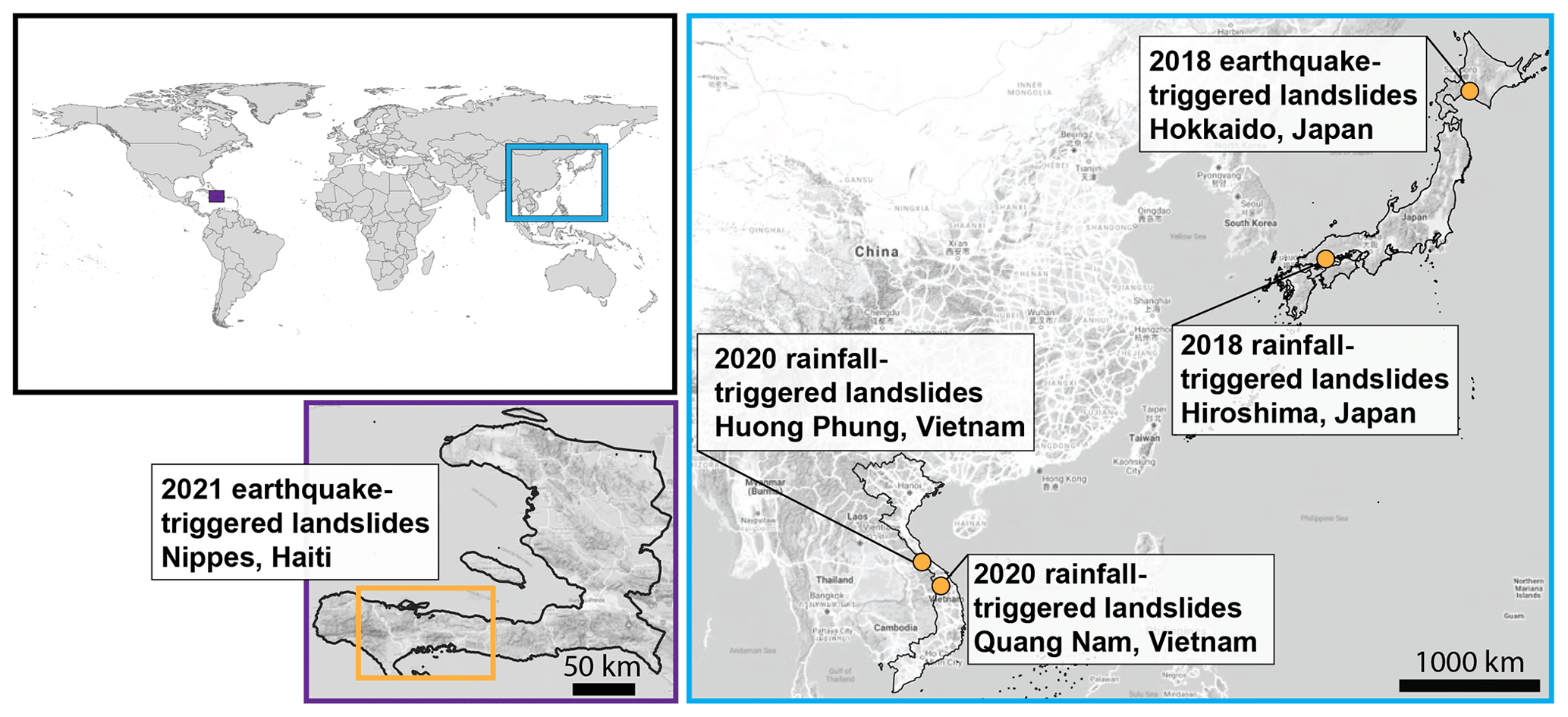
Figure 1 Google terrain map showing the location of landslide case studies. © Google Maps 2021.

2 Methods

The main goals of our work are to provide open-access tools in GEE that will enable users to utilize freely available SAR data to (1) detect areas that have likely experienced landslides as fast as possible after triggering events (i.e., rapid detection) and (2) identify landslides for event inventory mapping. We define “detection” and “mapping” using the framework described by Mondini et al. (2021), where detection is “the action of noticing or discovering single or multiple landslide failures in the same general area” and mapping “refers to the action of delineating the geometry of a landslide”.

The use of SAR data is particularly important when optical data are limited due to cloud cover. Our methodology is developed in the GEE “playground” (browser-based graphical user interface) using the JavaScript application programming interface (API) (Gorelick et al., 2017). This interface allows for coding, mapping/visualization, documentation, and more, and the products can be easily exported for offline analyses. The GEE codes developed here are published on GitHub and as shared GEE script links (see “Code and data availability”).

2.1 SAR backscatter in Google Earth Engine

We analyzed changes in the SAR backscatter from the S1 satellite constellation to detect ground surface changes associated with landslides. The S1 constellation currently consists of two satellites, S1A and S1B, launched in March 2014 and April 2016, respectively. Each satellite has a minimum 12 d revisit time for a given area. Using data from both satellites provides a minimum 6 d revisit time. The S1 satellites carry a C-band radar sensor with a wavelength of ∼ 5.6 cm. Depending on the location of the AOI, both ascending (asc) and descending (desc) S1 data may be available (see worldwide acquisition coverage, https://sentinel.esa.int/web/sentinel/missions/sentinel-1/observation-scenario last access: 4 March 2022). Currently, S1 data are the only SAR data available in GEE.

GEE provides Level-1 S1 Ground Range Detected (GRD) backscatter intensity coefficient (σ^∘) images. The backscatter coefficient is defined as the target backscattering area (radar cross-section) per unit ground area. All scenes are processed to remove thermal noise, have undergone radiometric calibration (but not radiometric terrain flattening), and are orthorectified using the Shuttle Radar Topography Mission (SRTM) digital elevation model (DEM) (Farr et al., 2007) or the Advanced Spaceborne Thermal Emission and Reflection Radiometer (ASTER) DEM for areas above 60^∘ latitude. All S1 GRD data values are provided in logarithmic units of decibels (dB) calculated as $\mathrm{10}\times {\log }_{\mathrm{10}}\left(\mathit{\sigma }{}^{\circ }\right)$. The backscatter coefficient is a measure that can be used to determine if the radar signal is scattered towards or away from the SAR sensor. The direction of scattering is primarily controlled by the geometry of the landscape relative to the radar look direction and the electromagnetic properties of the land cover. The GEE S1 GRD collection is updated daily and new data are uploaded to GEE within 2 d of them becoming available. GEE ingests all of the available ascending and/or descending images on the fly.

GEE provides GRD images with 10 m pixel spacing and up to four polarization modes: (1) vertical transmit/vertical receive (VV), (2) horizontal transmit/horizontal receive (HH), (3) vertical transmit/horizontal receive (VV + VH), and (4) horizontal transmit/vertical receive (HH + HV). HH and HV polarizations are mostly acquired in polar regions, which are thus unlikely to be useful for landslide detection. For this study we only used SAR data in the VH polarization. Cross-polarizations, such as VH and HV, are sensitive to forest biomass structure (Le Toan et al., 1992) and are therefore useful to identifying landslides in vegetated areas. We encourage users of our methods to explore the use of other polarizations.

2.2 Landslide detection approach

Our landslide detection approach requires the user to select an AOI and time period before (T_pre) and after (T_post) the event of interest (EOI). The AOI can be a small region or a large mountain range, and the EOI can last from seconds (e.g., earthquakes) to several days (e.g., storms). Thus, it is important to consider the spatial and temporal scale of the EOI when selecting the AOI, T_pre, and T_post. Furthermore, T_pre and T_post will vary depending on the goal of the project (i.e., rapid detection or constructing full event inventories).

To reduce noise from poor-quality data, we removed all pixels with values ≤ −30 dB (based on a recommendation from the GEE S1 Data Catalog). We also reduce transient noise and error by stacking images to create pre-event (I_pre) and post-event (I_post) backscatter intensity stacks. SAR data stacking has been shown to significantly improve the signal-to-noise ratio in SAR data (e.g., Cavalié et al., 2008; Zebker et al., 1997). Thus, the SAR image stacks provide backscatter data that are more representative of the pre- or post-event ground surface properties. Each stack was calculated as the temporal median of the pre-event and post-event SAR data. We constructed image stacks using ascending data, descending data, and combined ascending and descending data. The combined ascending and descending data (also referred to here as “asc and desc”) were calculated as the mean of the ascending and descending stacks.

We detected potential landslides by examining the change in the backscatter coefficient using the standard SAR intensity log ratio approach, I_ratio, defined as $I_{\mathrm{ratio}}=\mathrm{10}\times {\log }_{\mathrm{10}}(I_{\mathrm{pre}}/I_{\mathrm{post}})$ (e.g., Jung and Yun, 2020; Mondini et al., 2019, 2021). Because GEE provides the backscatter coefficient data in dB, I_pre−I_post is equivalent to the I_ratio (logarithm quotient rule). The I_ratio can be either positive or negative, with positive values corresponding to a decrease in the post-event SAR backscatter intensity. SAR backscatter changes following landslide events occur because landslides cause major changes in ground surface properties that alter the radar reflectance, hillslope geometry, roughness, and dielectric properties (Adriano et al., 2020; Mondini et al., 2021; Rignot and Van Zyl, 1993).

We also note that other ground surface change, for instance due to flooding, agriculture, mining, deforestation, and more, can also be detected by examining I_ratio (e.g., Jung and Yun, 2020; Tay et al., 2020) and may cause false positives. To help reduce false positives, we removed areas that are unlikely to correspond to landslides (e.g., small lakes, rivers, flat surfaces, hilltops) by using threshold-based masks made from the topographic slope and curvature calculated from the 1 arcsec (∼30 m) resolution NASADEM, which comprises reprocessed SRTM data with improved height accuracy and filled missing elevation data (NASA JPL, 2020). We refer to this mask throughout this paper as the “DEM mask”. Since landslides typically initiate on steep hillslopes, slopes of less than a few degrees can be masked, as these are the areas that generally correspond to non-landslide locations. However, slope thresholds will vary in different regions. Additionally, it is common for landslides to run out into lower-slope areas; therefore it is important to initially consider a wide range of slope values when searching for landslide deposits. We also mask out larger water bodies, including oceans and some lakes and river shorelines, using the water body data stored in the NASADEM layer.

2.3 SAR change detection performance and determination of most effective detection strategies

To determine the performance and most effective strategies of our SAR backscatter change detection for landslides, we performed both quantitative and qualitative comparisons with mapped landslide inventories and satellite optical imagery. We quantitatively evaluated our results with a previously published landslide inventory for the 2018 Hiroshima landslide event using receiver operating characteristic (ROC) curves (Fan et al., 2006). We provide a qualitative visual comparison with published landslide inventories for the 2018 Hiroshima, 2018 Hokkaidō, and 2021 Haiti landslide events and qualitative visual comparisons with S2 optical images for the 2018 Hiroshima, 2018 Hokkaidō, and 2020 Vietnam events. We note that in most cases, especially for rapid response, neither cloud-free optical images nor an external landslide inventory is likely to be available prior to investigation. In some cases, partial-cloud-cover optical images can be used to reveal some parts of landslides and help constrain identification of landslides from SAR data. Therefore, we also include S2 imagery in our GEE tools.

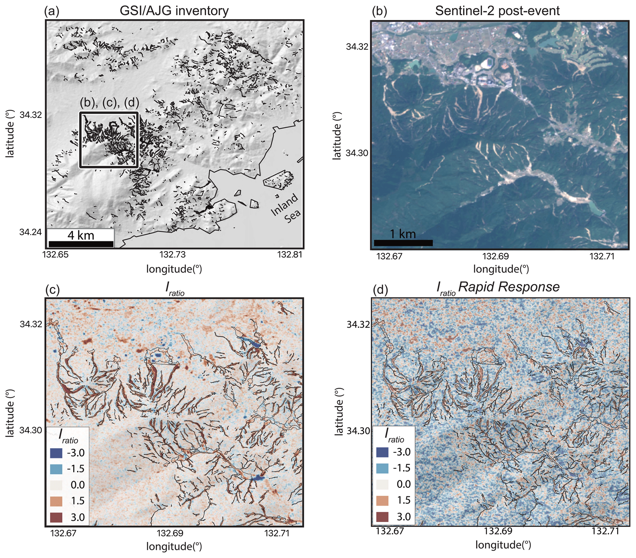
Figure 2 Rainfall-triggered landslides in 2018 in Hiroshima Prefecture. (a) NASADEM hillshade map with black polygons showing the GSI–AJG landslide inventory and the black box highlighting a sub-area of the AOI for plots (b)–(d). (b) Sentinel-2 optical image showing landslide scars. (c) SAR backscatter intensity change for combined ascending and descending stacks. SAR backscatter change maps were created from stacks made from 142 combined ascending and descending pre-event SAR images collected between 1 May 2015 and 29 June 2018 and 133 post-event SAR images collected between 9 July 2018 and 29 May 2020 and represent our best-case landslide identification. (d) SAR backscatter intensity change for simulated rapid response consisting of stacks made from the same 142 pre-event SAR images and 5 post-event SAR images collected between 9–24 July 2021. Red colors correspond to a decrease in post-event backscatter intensity (positive I_ratio values). Black polygons in (c) and (d) show the GSI–AJG landslide inventory. No DEM mask is applied to (c) or (d).

We quantified the success of our SAR backscatter change approach to identify true landslides for an extreme rainfall event that caused widespread landsliding in Hiroshima, Japan, in 2018. In this case study, we determined the detection performance using ROC curves, which measures our detection compared to an external landslide inventory under a variety of thresholds for discriminating between landslide and non-landslide pixels. We compared our SAR change detection to the landslide inventory made by the Geospatial Information Authority of Japan (GSI) and Association of Japanese Geographers (AJG) (see “Code and data availability”). To make a better comparison between our SAR change detection approach and the published landslide inventory, we manually removed landslides with an area < 100 m² from the GSI–AJG inventory for a better match with the minimum size of a 10 m × 10 m S1 SAR pixel. The ROC analyses were performed outside of the GEE platform using the MATLAB software package. We computed the ROC curves for all pixels within the ∼277 km² Hiroshima AOI shown in Fig. 2a. For these analyses, each pixel in the SAR intensity change raster was classified as a landslide if the I_ratio pixel value was greater than a threshold value or as non-landslide if it was less than the threshold value. The ROC curve is calculated by varying the I_ratio threshold values (I_TR). The initial I_TR,ROC is set as the minimum I_ratio value in the dataset and is increased until reaching the maximum value (thus we explore the entire range of I_ratio values). We then compared these classified pixels to the true landslides in the GSI–AJG inventory. For each threshold, the false positive rate, defined as the ratio of false positives to true non-landslide pixels, is compared to the true positive rate, defined as the ratio of true positives to true landslide pixels. The best performance is determined by maximizing the area under the ROC curve (AUC) (Fan et al., 2006). An AUC of 1 corresponds to a perfect classifier, while an AUC of 0.5 is equivalent to a random selection (50 % true positive rate and 50 % false positive rate). To maximize the AUC, we performed a sensitivity analysis by varying the pre-event and post-event time periods, the satellite acquisition geometry (i.e., asc, desc, or asc and desc), and the thresholds used for slope angle and curvature for the DEM mask. We then apply these lessons learned for optimal landslide detection strategies within the other case studies.

The main goal of our SAR change detection performance analysis was to determine the most effective detection strategies for landslide identification. While we validated and refined our landslide detection approach with external inventories and optical data in this study, it is important to emphasize that these external data are not required for landslide detection, and our tools are specifically designed to be used without an external landslide inventory and without optical data.

2.4 Landslide density heatmaps

To identify areas that have likely experienced landslides, which is particularly useful for rapid response, we implemented a landslide density heatmap approach. The heatmap is a data visualization technique that consists of a raster made by calculating the density of potential landslide pixels in a location over a given radius using a kernel density estimation. In this way, the landslide density heatmap is a proxy for potential landslide occurrence and not a heatmap of observed landslides classified using other methods. Several recent studies have applied a landslide density map approach to identify critically damaged areas, rather than focusing on the location of individual landslides (e.g., Bessette-Kirton et al., 2019; Burrows et al., 2020; Rosi et al., 2018). Our landslide density heatmaps are similar to these other density maps; however instead of counting individual landslides, we calculate the density of individually detected pixels over a fixed area. We define the pixels used in the heatmap by selecting an I_ratio threshold for heatmaps (I_TR,H). We manually explored I_TR,H using I_ratio percentiles to find the threshold value that visually highlights true landslides and reduces noise and false positives (see Sect. 4.2 for further explanation). All pixels ≥ I_TR,H are classified as potential landslide pixels, and all pixels below the threshold are excluded from the analyses. By using percentile-based thresholds, we are able to determine thresholds that correspond to landslides in different regions around the world. The I_TR,H is different from the thresholds used in the ROC–AUC analyses (I_TR,ROC) because I_TR,H must be defined without the use of an external landslide inventory.

We construct heatmaps using both GEE and QGIS. We use GEE to identify the potential landslide pixel locations and then export these as a KML file for heatmap construction in QGIS. Once in QGIS, the pixel locations are converted to a local UTM coordinate system, and then the heatmap is made using the Heatmap (Kernel Density Estimation) processing toolbox. The Heatmap toolbox requires selection of a radius, output raster size, and a kernel shape. We found good results with an output pixel size of 100 m and either a quartic or an Epanechnikov kernel shape. We did not identify a single best value to define the radius but generally found that radius values between ∼1–3 km were appropriate. We encourage users of our tools to explore the heatmap radius as it may vary depending on the AOI and EOI. In addition, we include an option to generate heatmaps directly in GEE.

3 Test sites

3.1 Rainfall-triggered landslides, 2018, Hiroshima, Japan

A record-breaking rainfall event occurred between 28 June and 8 July 2018 in west and central Japan that resulted in widespread floods and landslides. There were more than 200 fatalities, 20 000 damaged buildings, and 8500 damaged houses caused by these natural disasters. Hiroshima Prefecture had an especially high 108 fatalities, 14 862 damaged buildings, and 689 destroyed houses, significantly more than other prefectures, which was primarily due to the ∼8000 triggered landslides (Adriano et al., 2020; Hirota et al., 2019; Miura, 2019). Between 1–7 July 2018 there was approximately 500 mm of rainfall in Hiroshima Prefecture. Cloud cover prevented full landslide detection from optical images during the event period, and partial cloud cover remained for the month following the event.

The study AOI (Fig. 1) has a mixture of land cover including dense forest with little infrastructure in the mountains and farmlands and with residential areas and cities in the valleys. Within our ∼277 km² AOI, there were 3370 landslides mapped by the GSI–AJG. The minimum, mean, and maximum elevation is 0, 210, and 850 m, respectively. The mean slope angle is $\mathrm{14}{}^{\circ }\pm \mathrm{11}{}^{\circ }$ (± SD – standard deviation) with a maximum slope of 64^∘. Adriano et al. (2020) also used SAR intensity change with data from Advanced Land Observing Satellite-2 (ALOS-2) to successfully identify landslides for the same EOI.

3.2 Earthquake-triggered landslides, 2018, Hokkaidō, Japan

From 3–5 September, Typhoon Jebi passed over Japan, which brought about 100 mm of precipitation. A M_w 6.7 earthquake struck the Iburi–Tobu area of Hokkaidō Prefecture located in north Japan on 6 September 2018. The powerful ground motion (station HKD126 records up to 0.67 g; or 153 cm s⁻¹ peak ground velocity) caused liquefaction and triggered ∼6000 landslides, which destroyed and buried 394 buildings and killed 41 people (Yamagishi and Yamazaki, 2018; Zhang et al., 2019a). Most of the coseismic landslides were classified as coherent shallow debris slides (Zhang et al., 2019a). Due to cloud cover, full landslide detection from optical images was not available until 5 d later. Thus, optical imagery would have also been viable for rapid response for this event. Nonetheless, we use this EOI to test our GEE SAR-based detection tools.

We defined our study AOI (Fig. 1) as a 1170 km² region with a high landslide density (Zhang et al., 2019a). The land cover in our AOI includes dense forests in the mountains and farmlands and cities in the valleys. The minimum, mean, and maximum elevation is 0, 129, and 625 m, respectively. The mean slope angle is $\mathrm{10}{}^{\circ }\pm \mathrm{8}{}^{\circ }$ (±1 SD) with a maximum slope of 84^∘. This EOI was also previously investigated using SAR change detection methods by Adriano et al. (2020), Burrows et al. (2020), and Jung and Yun (2020). These studies showed that both coherence change and backscatter intensity change detection methods work to characterize the landslides; however the backscatter-based methods outperform SAR coherence change detection in the vegetated mountains (Jung and Yun, 2020).

3.3 Rainfall-triggered landslides, 2020, Huong Phung and Quang Nam, Vietnam

There were several major landslide events in Vietnam in October 2020 that were related to a particularly wet period between 6–28 October as the country was hit by six tropical cyclones (Van Tien et al., 2021). We examined landslide events from Huong Phung Commune on 18 October 2020 and Quang Nam Province on 28 October 2020 (Van Tien et al., 2021). We selected a 1080 km² AOI in Huong Phung and a 416 km² AOI in Quang Nam (Fig. 1). Cloud cover prevented full landslide detection from optical images during the event period, and partial cloud cover remained until February 2021.

The landslides in Huong Phung occurred in an area that had a mean slope angle of $\mathrm{17}{}^{\circ }\pm \mathrm{10}{}^{\circ }$ (±1 SD) with a maximum slope of 70^∘. The landslides in Quang Nam occurred in an area that had a mean slope angle of $\mathrm{21}{}^{\circ }\pm \mathrm{9}{}^{\circ }$ with a maximum slope of 71^∘. Both landslide areas in Vietnam are covered with dense forested vegetation and farmlands.

3.4 Earthquake-triggered landslides, 2021, Haiti

While writing this paper, a major M_w 7.2 earthquake struck on 14 August 2021 in Haiti and caused widespread landsliding in the southwestern part of the country (Martinez et al., 2021a). The earthquake epicenter was near Nippes, Haiti (∼120 km west of Port-au-Prince) (https://earthquake.usgs.gov/earthquakes/eventpage/us6000f65h/executive, last access: 4 March 2022). Heavy rainfall from Tropical Storm Grace further contributed to the disaster 2 d after the earthquake by triggering additional landslides and flooding and hindering the earthquake response (https://appliedsciences.nasa.gov/what-we-do/disasters/disasters-activations/haiti-earthquake-landslides-flooding-2021, last access: 4 March 2022). We were able to test our landslide detection approach in real time to support the response effort. We used our GEE tools to generate a landslide density heatmap for a ∼6500 km² region.

4 Results

We consider five independent landslide events to evaluate our method within Japan, Vietnam, and Haiti. We use the Hiroshima EOI to determine the most effective landslide detection strategies. We then apply our findings to the other test cases and make qualitative comparisons with cloud-free optical imagery and published landslide inventories (Hokkaidō and Haiti) to help assess the landslide detection performance.

4.1 Determining effective strategies for detecting landslides

To determine the most effective strategies for landslide detection with SAR backscatter change and to quantify detection success, we explored several different strategies and compared our findings with the GSI–AJG inventory for the 2018 Hiroshima event using the AUC scores computed from the ROC curves. These different strategies included changing the total number of SAR images used in the pre-event and post-event stacks; applying slope and curvature thresholds (i.e., DEM mask); applying I_ratio thresholds to highlight landslides and construct heatmaps; and using ascending, descending, or combined ascending and descending data. We define the “best-case” strategy as the approach that maximizes the AUC score.

First, we calculated the SAR backscatter change for the 2018 Hiroshima event using all of the SAR data that were available as of 29 May 2020 (when we began this study) to construct pre- and post-event stacks. The pre-event stack consisted of 142 images (100 ascending and 42 descending) with the first image collected 1152 d before the EOI and the last image collected 12 d before the EOI. The post-event stack consisted of 133 images (74 ascending and 59 descending) with the first image collected 1 d after the EOI and the last image collected 684 d after the EOI. Figure 2 shows the SAR-based backscatter change for a sub-area of our AOI. The SAR-based backscatter change shows many localized areas with I_ratio>2 that correspond to true landslides (Fig. 2c). These relatively high I_ratio areas have planform geometries typical of the debris flow type landslides (long, narrow, and channelized) that occurred during the 2018 rainfall event. We find most landslides have a positive I_ratio, i.e., I_post<I_pre, but there were also some places with negative I_ratio values within landslide scars as discussed in Adriano et al. (2020). Direct comparison with the cloud-free S2 optical imagery and the GSI–AJG inventory provided initial validation that SAR backscatter change can successfully detect landslides.

By comparing our change detection result with the GSI–AJG inventory, we found AUC scores of 0.7363, 0.7409, and 0.7712 for ascending, descending, and ascending and descending, respectively, using the complete pre- and post-event stacks. We repeated these analyses by changing the time duration for images included in T_pre and T_post to 12, 6, 3, and 1 months (Fig. 3). We varied the time span to simulate the impact of different quantities of available data for future studies. The highest AUC occurred when using all available pre-event and post-event data and by combining asc and desc data. We found that stacking large numbers of SAR images improves the signal-to-noise ratio.

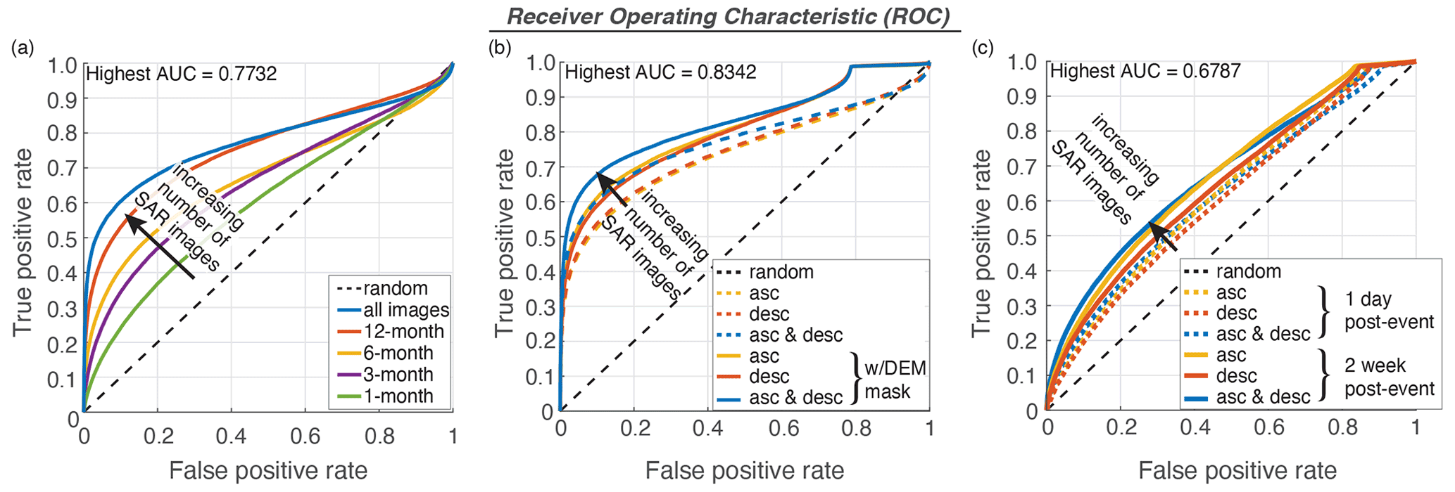
Figure 3 Receiver operating characteristic (ROC) analyses to determine the most effective strategy for landslide identification. (a) Colored lines show ROC curves as a function of the pre-event stack time period (T_pre) and post-event stack time period (T_post). (b) ROC curves using all available pre- and post-event data (highest AUC in a). Dashed colored lines correspond to ascending (asc), descending (desc), and ascending and descending data. Solid colored lines show the same data with the addition of the DEM mask slope and curvature thresholds. (c) ROC curves with DEM mask for rapid response detection using all pre-event SAR data and post-event data acquired 1 d and 1 week following the landslide event.

Next we used topographic data to help reduce false positives (Fig. 3b). To determine the slope and curvature thresholds, we used our most effective landslide identification strategy from the previous analyses (i.e., all available pre-event and post-event data) and found the slope and curvature thresholds that maximized the AUC. We found that we can further improve the AUC to 0.8101, 0.8041, and 0.8342 (best case) for asc, desc, and asc and desc, respectively, by using a DEM mask to exclude areas with low topographic slopes (<5^∘) and convex curvature ($>-\mathrm{0.005}$ m⁻¹). These areas of very low slope correspond to flat regions, such as cities and valley bottoms, and areas of relatively high positive curvature correspond to hilltops, where landslides are less likely to occur. Importantly, applying slope- and curvature-based masks makes a large improvement in landslide detection, but the specific slope and curvature threshold values will vary for other locations.

4.2 Determining effective strategies for rapid response

To identify landslides for rapid response (i.e., within 2 weeks of the landslide event), we applied the DEM mask from Sect. 4.1 and explored landslide detection scenarios where we have limited post-event data. Ideally, for rapid response, the first available image or first few available images following a catastrophic event will provide key information for identifying damaged areas. Thus, our methodology was designed with the goal of being able to provide information to responders on the location of critically damaged areas as quickly as possible.

For the 2018 Hiroshima simulated rapid response, we calculated the SAR backscatter change for a stack consisting of all of the available pre-event imagery and post-event imagery collected within 2 weeks of the EOI. The first post-event images were acquired on 10 July 2018 on both ascending and descending tracks, less than 1 d after the rainfall ended. By making comparison with the GSI–AJG inventory, we found an AUC of 0.6212 (Fig. 3c). The second set of post-event images was acquired on 16 July 2018 on both ascending and descending tracks. Incorporating four total post-event images improved the landslide signals and increased the AUC to 0.6787. Examination of the I_ratio within the landslides' areas shows some elongated debris flow shapes (Fig. 2d) but with a considerably lower signal-to-noise ratio when compared to using post-event stacks with many more images (Fig. 2c). Importantly, the AUC improves rapidly over the first week with the transition from two to four post-event images, indicating that the images immediately following the event provide key information on the location of damage for rapid response. While the AUC scores are relatively low for the rapid response analyses due to the low signal-to-noise ratio of the post-event images and it is challenging to identify individual landslides from the I_ratio, the SAR-based backscatter intensity change still provides key information that can be used to identify the critically damaged areas.

4.3 Landslide detection with SAR-based-change landslide density heatmaps

To rapidly detect areas with high landslide density, we developed a landslide density heatmap approach in GEE. As described above, the heatmap is a data visualization tool that uses the density of potential landslide pixels in a location over a given radius to generate a raster. A key step in generating a heatmap is to define the I_TR,H that classifies true landslide pixels. To select the best I_ratio threshold that corresponds primarily to true landslides, we examined data for the 2018 Hiroshima landslide event. We found that an I_TR,H value that includes all pixels ≥ the 99th-percentile value over the full AOI best highlights the true landslides and removes most of the false positives (Fig. 4; see Fig. A1 for other case studies). For both the simulated rapid response and the data stack that includes years of post-event data, the 99th percentile highlights true landslides while greatly reducing the false positives. Comparison with the 90th-percentile and 80th-percentile thresholds shows how the number of false positives increases rapidly by including a larger range of I_ratio values. We will use the 99th percentile as our I_ratio threshold for the remainder of the study.

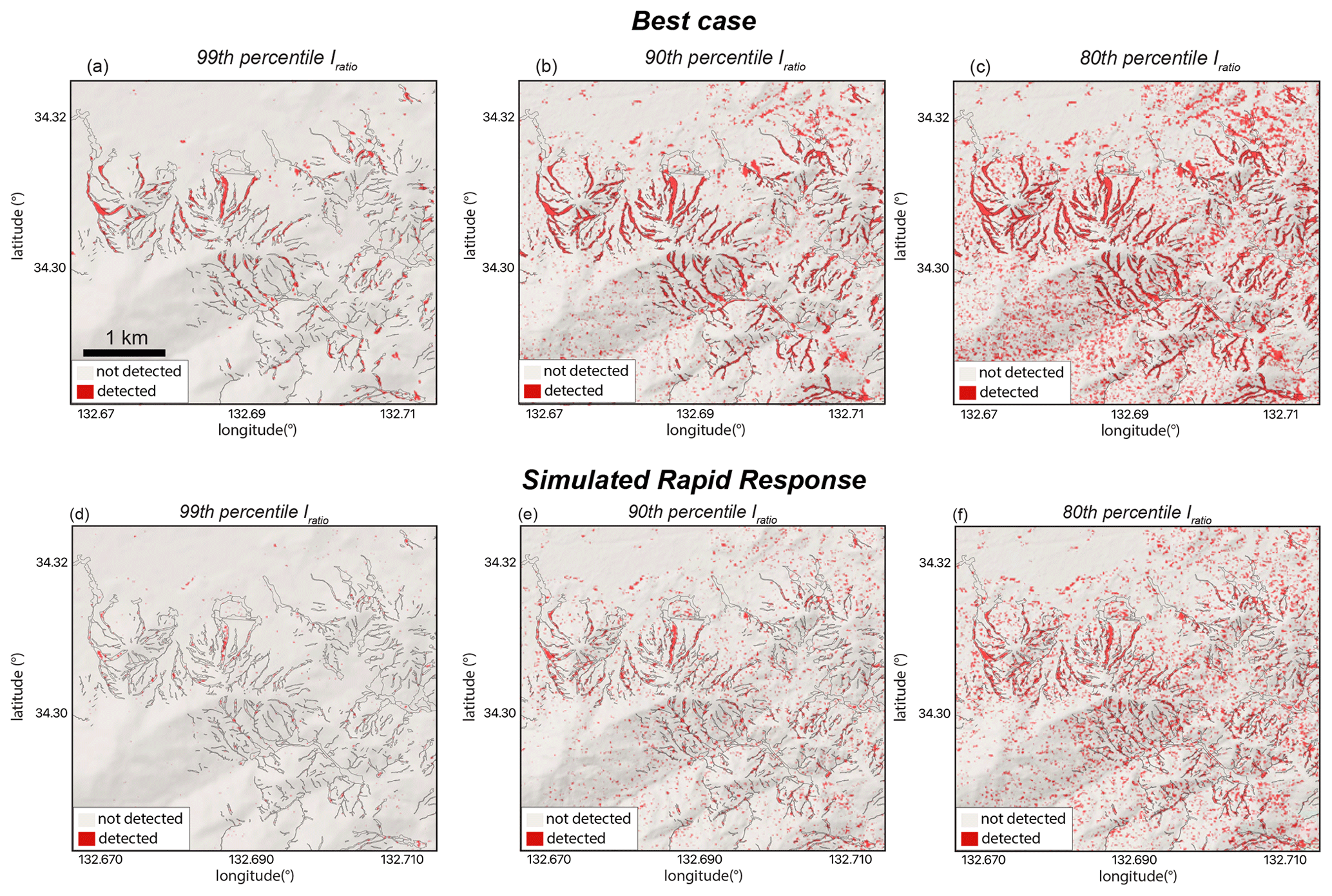
Figure 4 Detected landslides based on I_ratio threshold values (I_TR,H) for the 2018 Hiroshima landslide event. (a–c) The 99th-, 90th-, and 80th-percentile thresholds for detecting landslides for the best-case landslide detection strategy that consists of stacks made from 142 combined ascending and descending pre-event SAR images collected between 1 May 2015 and 29 June 2018 and 133 post-event SAR images collected between 9 July 2018 and 29 May 2020. (d–f) The 99th-, 90th-, and 80th-percentile thresholds for detecting landslides for the simulated rapid response that consists of stacks made from the same 142 pre-event SAR images and 5 post-event SAR images collected between 9–24 July 2021. Images are draped over NASADEM hillshade. DEM mask is used to remove low topographic slopes (<5^∘) and convex curvature ($>-\mathrm{0.005}$ m⁻¹). Thin black polygons show the GSI–AJG landslide inventory.

Figure 5 shows our landslide density heatmap for the simulated rapid response scenario for the 2018 Hiroshima EOI. The heatmap highlights that the areas critically damaged by landslides, as shown by comparison with the GSI–AJG inventory, can be located within 2 weeks of the landslide-triggering event. Areas with bright red colors correspond to the areas with the highest potential landslide density and/or the largest landslides.

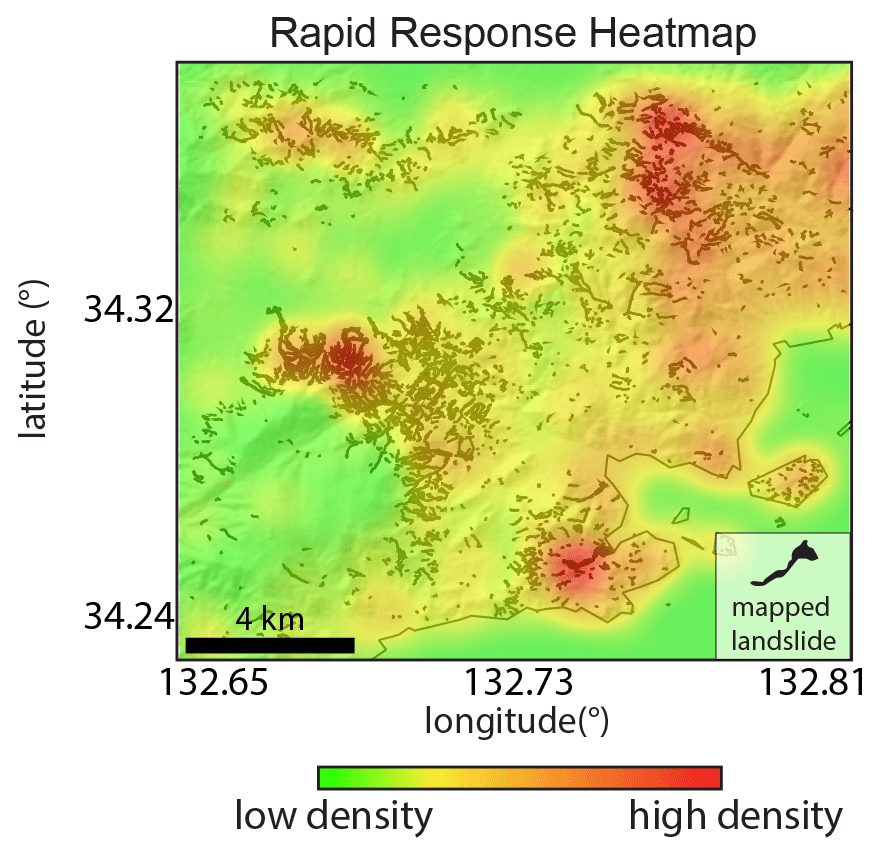
Figure 5 Simulated rapid response heatmap for the 2018 Hiroshima landslide event. Heatmap with red colors showing a high density of potential landslides draped over NASADEM hillshade. Black polygons are from the GSI–AJG inventory. Pre-event stack created from 142 combined ascending and descending SAR images collected between 1 May 2015 and 29 June 2018 and post-event stack created from 5 SAR images collected between 9–24 July 2021. Heatmap radius set to 1 km. DEM mask is used to remove low topographic slopes (<5^∘) and convex curvature ($>-\mathrm{0.005}$ m⁻¹).

4.4 Other case studies

Our analyses of the 2018 Hiroshima event provide us with useful guidelines for landslide detection and rapid response. To further test our approach, we applied our most effective strategies for rapid response to the 2018 earthquake-triggered landslides in Hokkaidō, Japan, and 2020 rainfall-triggered landslides in Huong Phung and Quang Nam, Vietnam. Our most effective strategies include using a DEM mask and a large pre-event stack of combined ascending and descending data. We note that the specific values for the DEM mask will vary from location to location, so we recommend exploring a range of values. For these case studies, we simulated rapid response scenarios by limiting T_post to 2 weeks of the EOI.

4.4.1 Simulated rapid response for the 2018 earthquake-triggered landslides, Hokkaidō, Japan

We defined the simulated rapid response scenario pre-event time period between 1 August 2015 and 5 September 2018 and the post-event time period between 6–21 September 2018 for the Hokkaidō event. These time periods resulted in a pre-event stack with 150 combined ascending and descending images and a post-event stack with 3 combined ascending and descending images. We found that the rapid response heatmap characterized the areas with high landslide density (Fig. 6a). Direct visual comparison with the published inventory from Zhang et al. (2019a) shows good agreement between the areas detected by our SAR backscatter change heatmap and the true landslides. Figure 6b–d show a close-up of an area with a particularly high landslide density. The I_ratio values and the I_ratio ≥ the 99th percentile show strong and clear signals that correspond to true landslides. In addition, the I_ratio values ≥ the 99th percentile appear to correspond almost entirely to true landslides, and examination of the 99th-percentile map and heatmap allows for straightforward landslide detection.

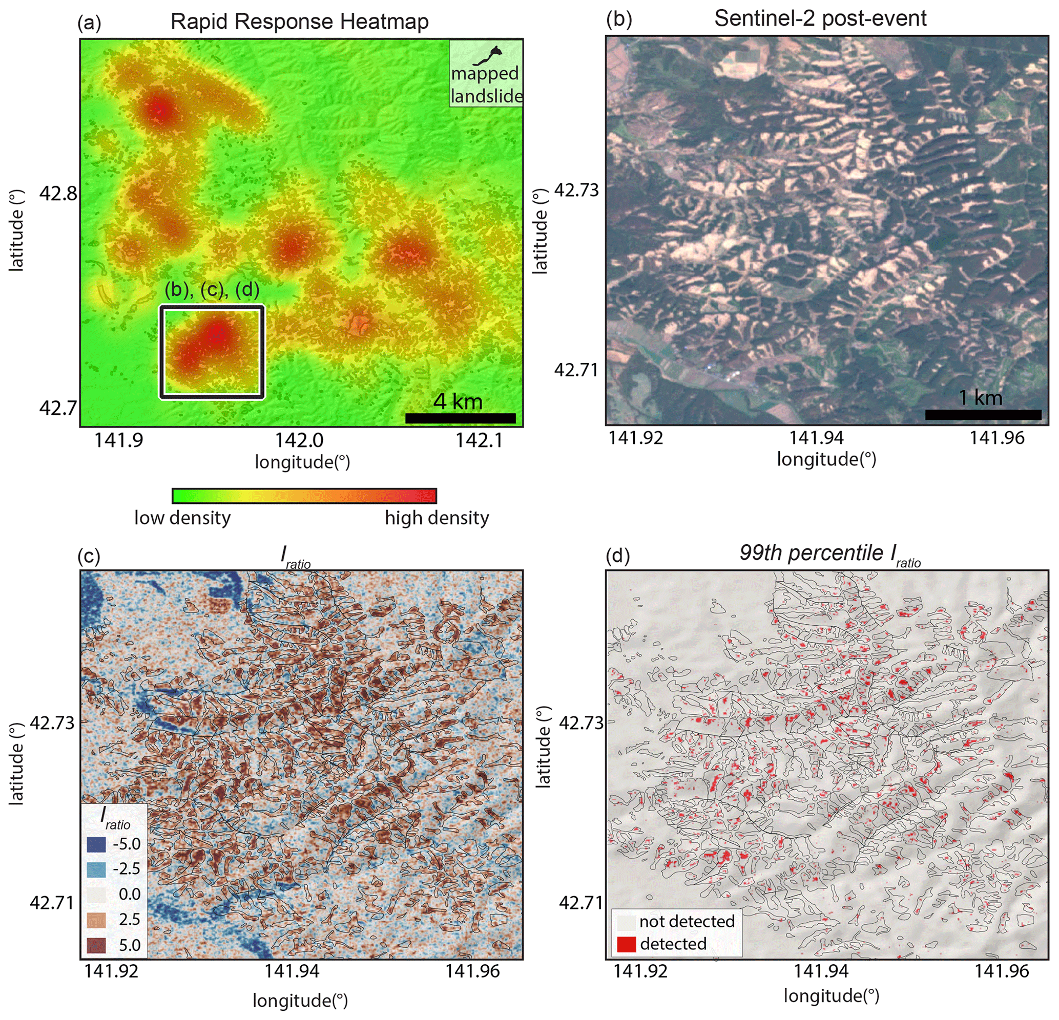
Figure 6 Simulated rapid response heatmap for the 2018 Hokkaidō landslide event. (a) Heatmap with red colors showing a high density of detected landslides draped over the NASADEM hillshade. Heatmap radius set to 1 km. (b) Post-event Sentinel-2 optical image for sub-area shown in (a). (c) I_ratio map for sub-area draped over the NASADEM hillshade. (d) I_ratio threshold map with red pixels that are ≥ the 99th-percentile I_ratio draped over the NASADEM hillshade. Black landslide polygons in (a), (c), and (d) are from Zhang et al. (2019a). SAR images are made from stacks consisting of 150 pre-event SAR images collected between 1 August 2015 and 5 September 2018 and 3 post-event SAR images collected between 6–21 September 2018. DEM mask is used to remove low topographic slopes < 10^∘ in (a) and (d). No curvature mask is used because the landslides appear to have been sourced from hilltops.

4.4.2 Simulated rapid response for 2020 rainfall-triggered landslides, Huong Phung and Quang Nam, Vietnam

We constructed landslide density heatmaps for simulated rapid response for the October 2020 landslide events in AOIs in Huong Phung (Fig. 7) and Quang Nam (Fig. 8), Vietnam. There were hundreds of landslides triggered during this unusually wet period, but no published inventory of them is currently available (to our knowledge). For the Huong Phung event, we defined the pre-event period as between 1 October 2016 and 17 October 2020 and the post-event period as between 19 October and 1 November 2020. This resulted in 229 combined ascending and descending pre-event SAR images and 4 post-event SAR images. For the Quang Nam event, we defined the pre-event period as between 1 October 2016 and 27 October 2020 and the post-event period as between 29 October and 7 November 2020. This resulted in 253 combined ascending and descending pre-event SAR images and 4 post-event SAR images. The heatmaps for both events clearly show areas with high density of detected landslides. We checked areas on the heatmaps that showed high landslide density by comparing pre- and post-event S2 optical imagery (Figs. 7 and 8). The optical imagery shows that the heatmaps successfully highlighted areas with high landslide density. We also observed some false positives in the heatmap for the Huong Phung area. We observed apparent high landslide density that appeared to correspond to false positives related to clearcutting of trees (Fig. 7e).

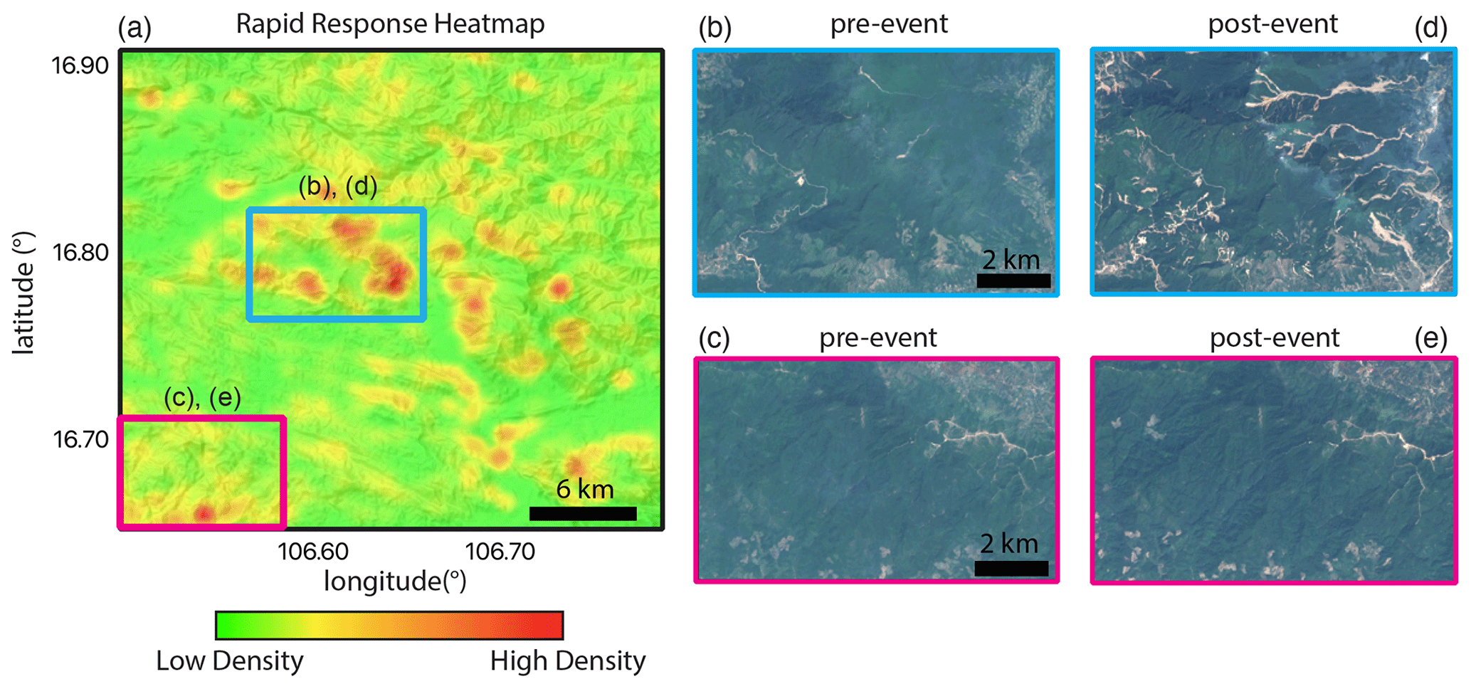
Figure 7 Simulated rapid response heatmap for Huong Phung, Vietnam. (a) Heatmap draped over the NASADEM hillshade of the topography with red colors corresponding to areas with high potential landslide density. Heatmap made from stacks consisting of 229 pre-event SAR images collected between 1 October 2016 and 17 October 2020 and 4 post-event SAR images collected between 19 October and 1 November 2020. Heatmap radius set to 1 km. DEM mask is used to remove low topographic slopes < 10^∘ and convex curvature > −0.005 m⁻¹. Blue and magenta rectangles show zoomed-in areas in figures (b)–(e). Pre-event (b, c) and post-event (d, e) Sentinel-2 optical images for high–landslide-density and low-landslide-density zones identified with the heatmap. High-density zones in (c) and (e) appear to correspond to deforestation.

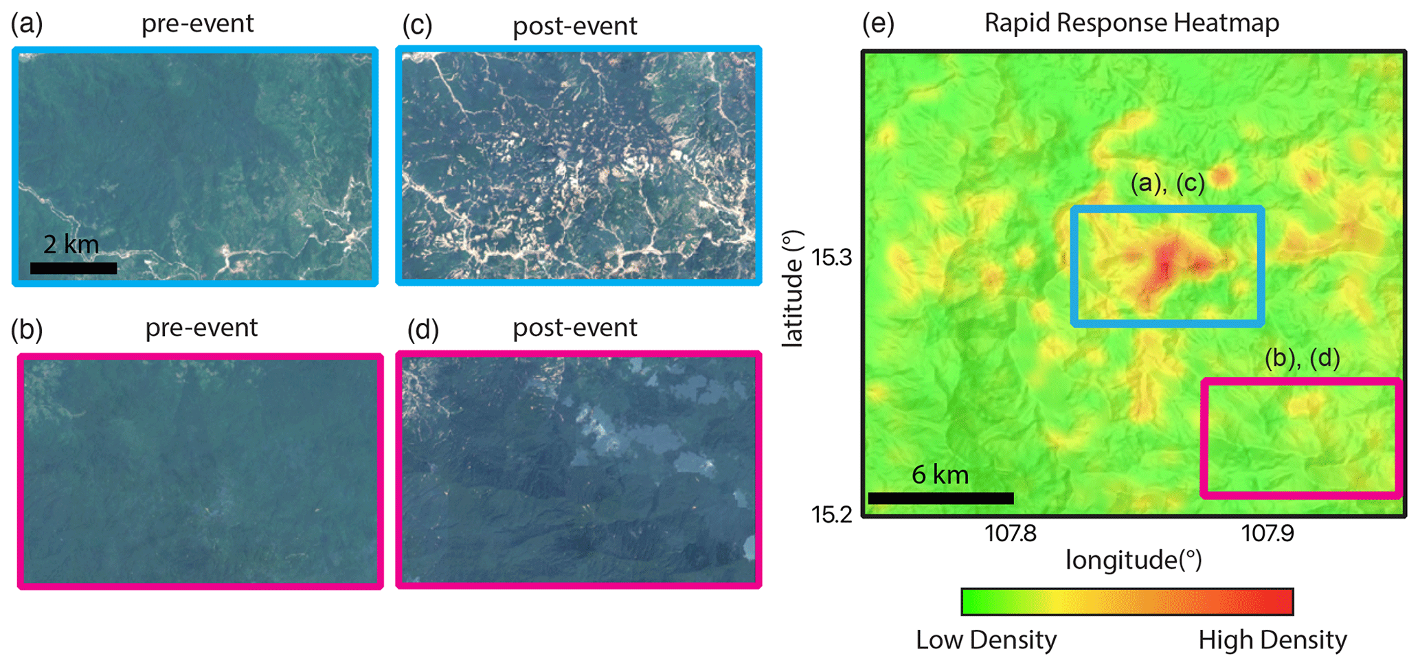
Figure 8 Simulated rapid response heatmap for Quang Nam, Vietnam. (a–d) Pre- and post-event Sentinel-2 optical images for high-landslide-density and low-landslide-density zones identified with the heatmap. (e) Heatmap draped over the NASADEM hillshade of the topography with red colors corresponding to areas with high potential landslide density. Heatmap made from stacks consisting of 253 pre-event SAR images collected between 1 October 2016 and 27 October 2020 and 4 post-event SAR images collected between 29 October and 7 November 2020. Heatmap radius set to 1 km. DEM mask is used to remove low topographic slopes < 10^∘ and convex curvature > −0.005 m⁻¹. Blue and magenta rectangles show zoomed-in areas in (a)–(d).

4.5 Application of landslide density heatmaps to support rapid response for 2021 Haiti earthquake

On 15 August 2021, just 1 d after the 2021 Nippes, Haiti, M_w 7.2 earthquake, we used our GEE tools to generate a landslide density heatmap. Our heatmap only includes the landslides triggered by the earthquake and not those triggered by Tropical Storm Grace 2 d later. We defined the pre-event period as between 1 August 2017 and 13 August 2021 and the post-event period as between 14–15 August 2021. This resulted in 104 descending pre-event SAR images and 1 descending post-event SAR image. Note that because there was only a single descending image collected immediately after the event, we used a descending-only stack to create the heatmap. We found an area of high landslide density located ∼ 56 km west of the epicenter (Fig. 9a). We posted our landslide heatmap on the NASA Disasters Mapping Portal (https://maps.disasters.nasa.gov/arcgis/apps/MinimalGallery/index.html?appid=3b785d8e1ff943e59a9810f67181b8d3, last access: 4 March 2022) on 17 August 2021, where numerous other remote sensing datasets were hosted including the SAR coherence-based damage proxy map (DPM) and coseismic S1 interferogram that were produced by the Advanced Rapid Imaging and Analysis (ARIA) team at NASA's Jet Propulsion Laboratory and California Institute of Technology in collaboration with the Earth Observatory of Singapore (EOS). The SAR-based products are particularly important because cloud cover prevented full optical-based landslide mapping for weeks after the earthquake (Martinez et al., 2021a).

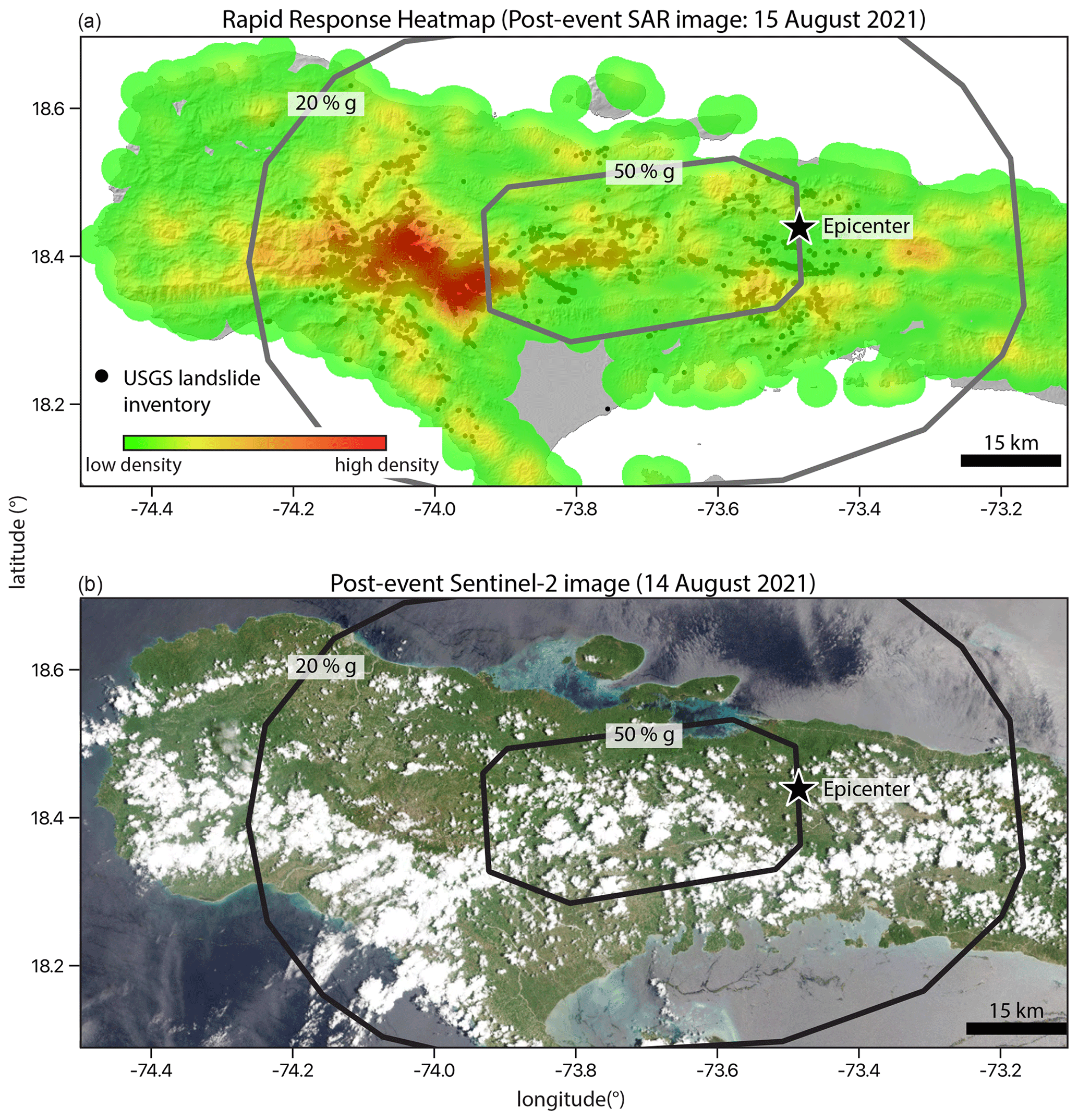
Figure 9 Real-time rapid response heatmap for the 2021 earthquake-triggered landslides in Haiti. (a) Landslide heatmap draped over the NASADEM hillshade of the topography with red colors corresponding to areas with high potential landslide density. Heatmap made from stacks consisting of 104 descending pre-event SAR images collected between 1 August 2017 and 13 August 2021 and 1 descending post-event SAR image collected on 15 August 2021. Heatmap radius set to 3 km. DEM mask is used to remove low topographic slopes < 10^∘. Dark circles show the USGS landslide inventory (Martinez et al., 2021a). (b) Post-event Sentinel-2 optical imagery showing high cloud cover on the day of the earthquake. (a, b) Black star shows the M_w 7.2 earthquake epicenter, and contours show the peak ground acceleration data as a percentage of gravity (g) provided by the USGS (see “Code and data availability”).

The first available optical-based landslide inventory was produced on the day of the earthquake (14 August 2021) using a heavily cloud covered S2 image (Fig. 9b) with the Semi-Automatic Landslide Detection (SALaD) approach (Amatya et al., 2021). Due to the cloud cover, only a ∼300 km² area had partial visibility, and ∼525 landslides were mapped (https://maps.disasters.nasa.gov/arcgis/apps/MinimalGallery/index.html?appid=3b785d8e1ff943e59a9810f67181b8d3, last access: 4 March 2022). The USGS then released a larger preliminary rapid landslide inventory that included 3625 landslides over a ∼5000 km² area between 17–23 August 2021 made from Planet and Maxar optical imagery and published a final inventory of 4893 landslides made from Sentinel-2, WorldView, and Planet imagery in December 2021 (Martinez et al., 2021a; see “Code and data availability”). We found good agreement between our SAR-based landslide heatmap and the area of highest landslide density mapped with optical imagery, providing further evidence that our SAR-based approach is well suited for rapid response following major catastrophic landslide events (Fig. 9a). A comparison of different landslide datasets and methodologies to support the response and recovery effort is ongoing and will be the topic of future work.

5 Discussion

5.1 Landslide detection using SAR backscatter change

Our results show that SAR-based backscatter intensity change in GEE can be used to detect landslides over large areas. The main goal of this study was to develop a methodology for those without SAR expertise or specialty processing software that can be used to create landslide density heatmaps that can aid in rapid response to catastrophic landslide events. We performed sensitivity tests and quantitative analysis for the 2018 Hiroshima landslide event in order to help guide future investigations that do not have an external landslide inventory to help refine their approach. We demonstrated that the landslides in Hiroshima Prefecture, as well as the other case studies, caused an overall decrease in the SAR backscatter coefficient, which resulted in a relatively large positive I_ratio (Figs. 2 and A2). Furthermore, we found that the true landslides are well characterized by I_ratio values that are ≥ the 99th percentile (Figs. 4 and 6d).

We found that increasing the total number of SAR images used in the SAR backscatter intensity stacks improved landslide detection performance (Fig. 3). Our study also confirms findings of previous work (e.g., Adriano et al., 2020) that the detection performance was further improved by applying a DEM mask to remove areas where landslides were unlikely to occur. Additionally, combining ascending and descending geometry SAR data into a single stack together improved landslide detection when compared to using ascending or descending data individually (Fig. 3). Combining ascending and descending data into a single stack helps reduce bias introduced from the acquisition geometry (e.g., radar shadows, foreshortening, layover). The combined effect of stacking hundreds of images with both geometries can improve the ability to detect landslides. Our findings indicate that future catastrophic events will benefit from a large number of pre-event images (S1 data have been collected since 2014). However, there is likely a point at which there are diminished returns on adding additional pre-event data because of increased computation time. Additionally, we expect further improvements in landslide detection as more advanced SAR processing methods are incorporated into GEE. A recent GEE toolset by Mullissa et al. (2021) implements border noise correction, speckle filtering, and radiometric terrain normalization into the S1 data that may improve our landslide detection capability, but these methods are not yet incorporated into our GEE tools.

The landslide type and size also appear to impact our landslide detection performance. The minimum pixel size of the S1 GRD data is 10 m, with a pixel resolution of ∼3 and 22 m. This resolution limits our ability to detect small landslides with lengths or widths < 20 m, and as a result larger landslides are more likely to be detected. Furthermore, users should exercise caution interpreting individual pixels that are isolated in space as landslides. Landslides are most often constituted by clusters of nearby pixels. Therefore, SAR change detection with S1 data will work better in areas with larger landslides, such as the 2018 Hokkaidō landslide event. The type of landslide also impacts the detection success and must be considered when setting slope and curvature thresholds. Detection of channelized landslides, such as debris flows, benefits from curvature thresholds that remove convex hillslopes from the analyses, while rockslides or translational landslides may initially occur along convex hillslopes (e.g., 2018 Hokkaidō landslide event). Additionally, removing areas with low slope angles may remove the landslide deposit from the detection analyses. Therefore, we suggest performing landslide detection with a range of slope and curvature thresholds for each specific field area.

The next step after identifying landslide areas is to construct landslide inventories. The ability to construct accurate landslide inventories generally improves with time when additional post-event SAR images are collected. GEE has drawing tools that can be used to add a marker (i.e., point location) or draw a line, polygon, or rectangle. Data from GEE, such as SAR backscatter change maps, can also be easily exported as GeoTIFF files for mapping in GIS software. Although not fully explored in this work, we have added a threshold-based approach that classifies pixels with certain I_ratio values as landslides and can be used for mapping. This is the same I_ratio threshold used to make the heatmaps (I_TH,H). This approach is included in our GEE toolset (see “Code and data availability”). We also note that GEE has machine learning capabilities that can be used to help identify landslides.

5.2 Landslide density maps

Landslide density maps have been used to identify spatial trends in landslide occurrence and to identify areas that were critically damaged during landslide events (e.g., Bessette-Kirton et al., 2019; Burrows et al., 2020; Rosi et al., 2018). These density maps are also well suited for rapid response because they do not require detailed and time-consuming mapping. Additionally, landslide density maps can also be compared or combined with empirical landslide susceptibility models, which typically operate with a coarse resolution (kilometer-scale pixels), to further refine landslide detection capabilities (Burrows et al., 2021).

Landslide density maps are typically made by counting the number of landslides within a fixed area. For example, Bessette-Kirton et al. (2019) used a 2×2 km grid with optical satellite imagery and assigned high landslide density to >25 landslides, low landslide density to 1–25 landslides, or no landslides for landslides triggered during Hurricane Maria in Puerto Rico, USA. Burrows et al. (2020) used SAR coherence change with S1 and ALOS-2 data at a $\sim \mathrm{200}\times \mathrm{220}$ m resolution to generate coherence change density maps for landslides triggered by the 2015 M_w 7.8 Gorkha, Nepal, earthquake; the 2018 M_w 6.7 Hokkaidō, Japan earthquake; and two 2018 Lombok, Indonesia, earthquakes of M_w 6.8 and 6.9.

Our landslide density heatmap approach is similar to other density maps; however instead of counting individual landslides, we calculate the density of individually detected pixels over a fixed area. That means that the landslide density is calculated at the sub-landslide scale. One major advantage of our heatmap approach with SAR change detection in GEE is that the processing can be done within a short period of time (normally within a few minutes) once the post-event SAR imagery is available in GEE. The results can be easily interpreted and can highlight areas with the highest amount of change detection. Furthermore, this method can be easily integrated with population density or land use maps to further prioritize rescue missions after a significant landslide event. For the landslide EOIs we examined, we found our heatmap approach was able to highlight areas with high landslide density for the real-time (Haiti) and simulated (Japan and Vietnam) rapid response scenarios.

5.3 Challenges with rapid response landslide detection

Despite the overall success of our case studies, we acknowledge there are many challenges when attempting to detect landslides for rapid response. In this section, we focus on the challenges and possible sources of error in the rapid response products. The main challenges of rapid response include the following: (1) uncertain location and size of AOI, (2) SAR backscatter intensity changes that do not correspond to true landslides, and (3) computational limitations in GEE.

5.3.1 Identifying the AOI and EOI

One major consideration for rapid response is correctly identifying the correct AOI and EOI for the investigation. This is not a straightforward endeavor, and our work here has certainly benefited from performing retrospective analyses with known EOIs and AOIs (except for Haiti). For rapid response, prompt identification of the location and the scale of an event soon after a disaster is difficult, and therefore the location and the size of AOI are likely to be somewhat unknown. To help identify the AOI and EOI for rapid response in real time, we recommend consulting the International Charter Space and Major Disasters (https://disasterscharter.org/, last access: 4 March 2022) and/or blogs such as The Landslide Blog (https://blogs.agu.org/landslideblog/, last access: 4 March 2022). Furthermore, depending on the event, additional information can also be used to identify the AOI. For example, for rainfall-triggered landslides, satellite-based precipitation estimates, such as those provided by the Global Precipitation Measurement (GPM) mission or from the European Centre for Medium-Range Weather Forecasts (ECMWF), can be useful in identifying regions with higher landslide susceptibility (these products are also available in GEE). There are also freely available global landslide models that aim to identify likely landslide areas in near real time. Kirschbaum and Stanley (2018) identified potential landslide areas with the Landslide Hazard Assessment for Situational Awareness (LHASA) model, which combines satellite-based precipitation estimates from GPM with a global landslide susceptibility map. A second version upgraded LHASA from categorical to probabilistic outputs (Stanley et al., 2021). LHASA version 2.0 also estimates the potential exposure of population and roads to landslide disasters (Emberson et al., 2020). These exposure estimates could conceivably be used to identify the locations where landslides are most likely to have severe impacts. Our heatmap approach could benefit from guidance and comparison with predictions or “nowcasts” from LHASA. For earthquake-triggered landslides, the users can incorporate ShakeMaps and Ground Failure earthquake products produced by the US Geological Survey and set the AOI to cover the regions with high predicted ground failure or with high peak ground acceleration. We implemented this strategy successfully for the 2021 Haiti event. Additionally, consideration of population density or township maps can be used to help determine an AOI.

5.3.2 Challenges using the landslide heatmap

We found our heatmap approach can be used to identify areas with high landslide density. In order to construct a heatmap, we had to select an I_ratio threshold (I_TH,H), kernel density shape, and kernel density radius. We found that an I_TH,H ≥ the 99th percentile of the entire AOI characterized the true landslides in all case studies. However, because the I_TH,H is based on the 99th-percentile value of the entire AOI, by definition the heatmap will always highlight some pixels (e.g., false positives) even if there is no landslide event. In many cases, these false positives will be related to natural and human-made ground surface change, including but not limited to deformation from mining, construction, deforestation, agriculture, flooding, snow cover, and changes in reservoir water levels. We observed numerous places where SAR backscatter coefficient change is not related to landslides (Figs. 2c and d, 4, 6c and d). The DEM mask helps remove some, but not all, of these false positives. Land use/cover maps have also been successfully implemented to help reduce false positives (e.g., Adriano et al., 2020) but have not been applied in our work. If there is no actual ground deformation in the AOI, we expect the 99th-percentile pixels to be randomly distributed, and therefore the heatmap will not highlight a specific region. We are not able to directly assess the number of false negatives with the heatmap because this approach is not used to map individual landslide polygons.

To further explore potential issues with our heatmap approach, we constructed a heatmap for our Hokkaidō AOI during a period of time with no known landslide events just prior to the Iburi earthquake (Fig. 10). We set the pre-event time period from 1 August 2015 to 5 June 2018 and the post-event time period from 6–21 June 2018. Our heatmap detected a large area near the center of the AOI. Upon further inspection, we found this change in backscatter intensity was related to the filling of a large reservoir. The reservoir was not entirely masked out of our heatmap because the edges of the reservoir area have slopes > 10^∘. While we expect false positives to exist using this method, we show that overall, the high density of ground surface change after a known landslide-triggering event points to the overarching spatial distribution of landslides.

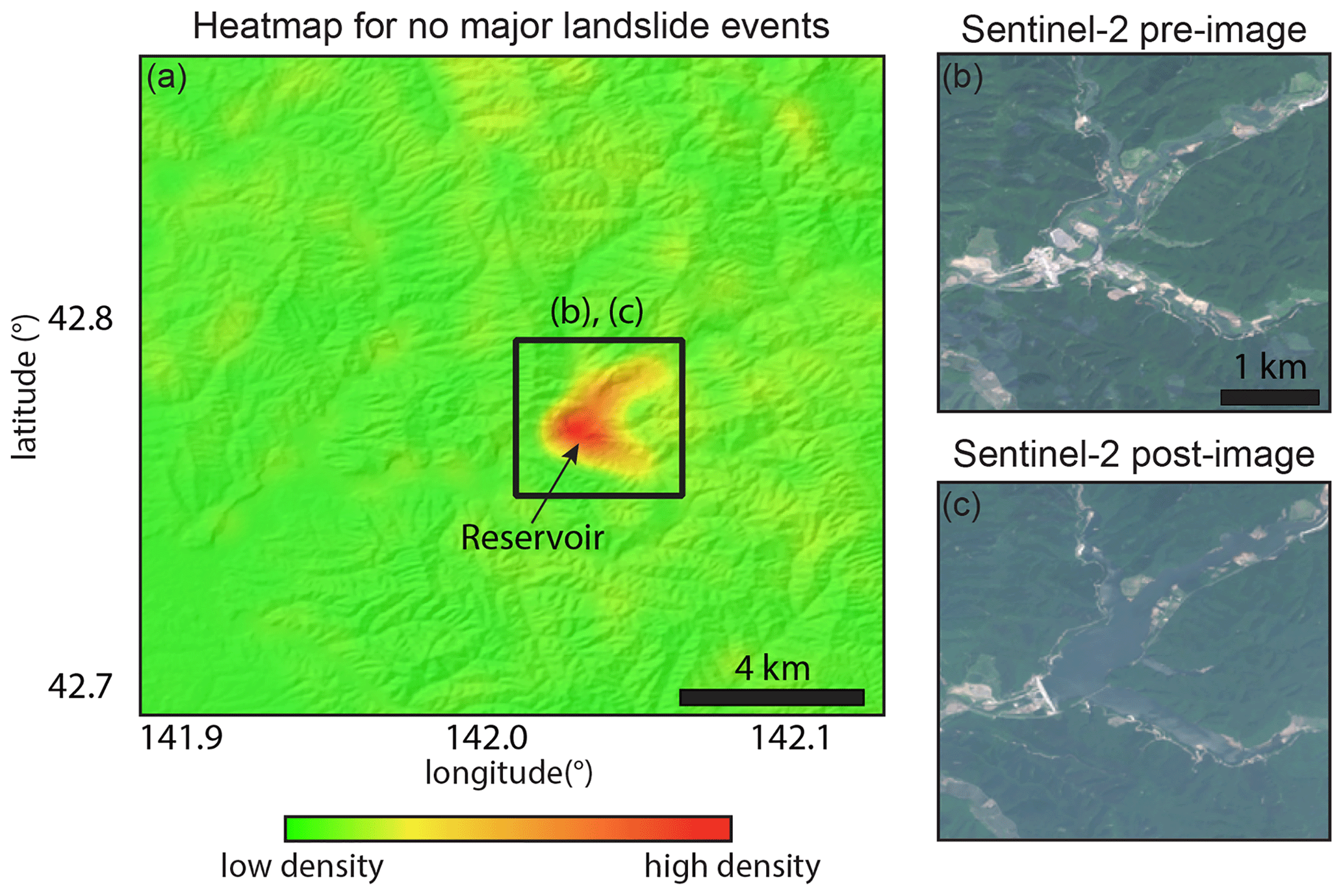
Figure 10 Heatmap made during a period with no major landslide events in Hokkaidō, Japan. (a) Heatmap draped over the NASADEM hillshade with red colors corresponding to areas with high density of ground surface change. Heatmap made from stacks consisting of 127 pre-event SAR images collected between 1 August 2015 and 6 June 2018 and 5 post-event SAR images collected between 6–21 June 2018. Heatmap radius set to 1 km. High-density region in heatmap corresponds to true ground surface change related to infilling of a large reservoir. Because the reservoir perimeter has slopes > 10^∘, it was not masked out of our analyses. (b, c) Pre- and post-image Sentinel-2 optical images showing the infilling of the reservoir.

5.3.3 Computation limits in GEE

Although GEE enables analyses of large quantities of data, it is a shared cloud computing resource and as such has user limits. GEE restricts the total number of simultaneous processing requests and the maximum duration of requests and computational memory (Gorelick et al., 2017). Thus, computational issues can arise in GEE when trying to process extremely large datasets (>500 images) over large areas (>3500 km²). To overcome these issues, we suggest starting with small AOIs and then enlarging the AOI or using multiple AOIs instead of one large single AOI. Additionally, for events that occur after 2021, there are a large number of pre-event data that may be redundant and only increase computational time. Thus, we suggest limiting the pre-event time period to <4 years.

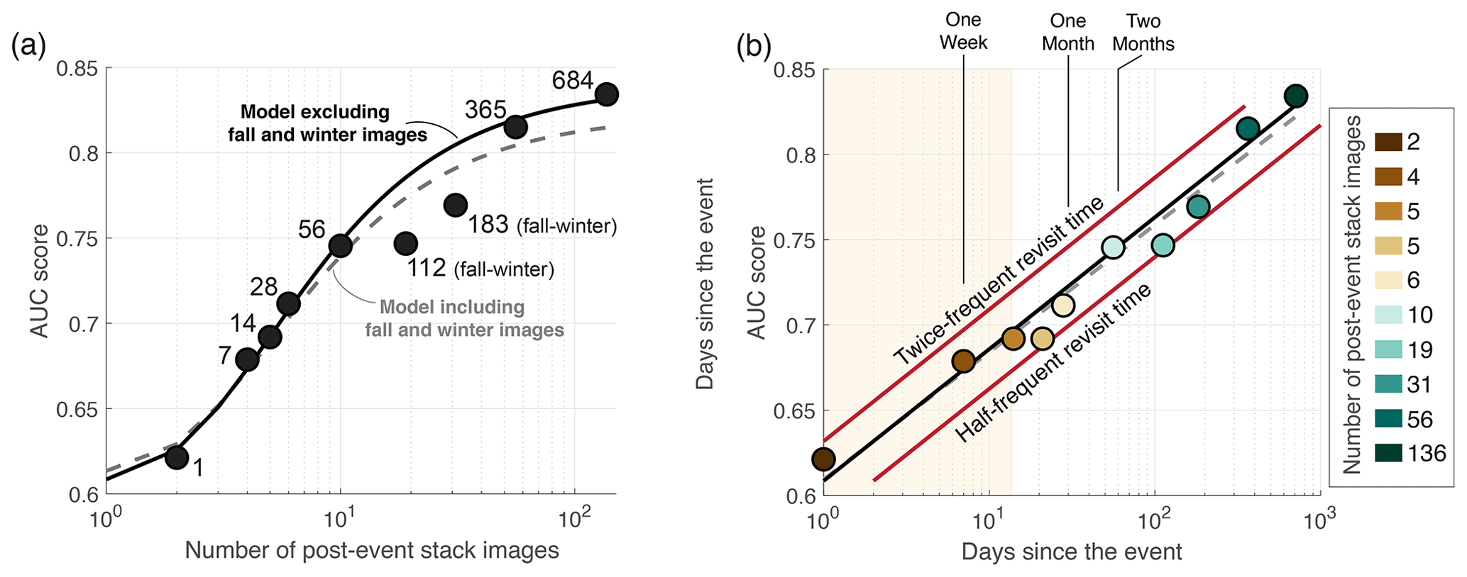
Figure 11 Area under the curve (AUC) score as a function of the increasing number of days and SAR images following the Hiroshima landslide event. (a) AUC score as a function of the number of SAR images used in the post-event stack. Dashed and solid black lines show exponential fit models with and without fall–winter SAR images, respectively. The rate of AUC increase decays exponentially with the number of images in the stack. Numbers next to black circles correspond to the number of days since the landslide event. The two fall–winter-labeled SAR images fall off the best-fit line, which we infer is due to seasonal differences in SAR backscatter intensity. (b) AUC score as a function of days since the Hiroshima landslide-triggering event. The dashed line shows the AUC score fit model, and the black line shows a model fit excluding fall–winter images. The light orange rectangle highlights the 2-week-long rapid response time period. The red lines indicate the predicted AUC score time series by assuming a satellite revisit time that is twice or half the S1 satellites for this region. The color scale corresponds to the number of images used in the post-event stack.

5.4 Satellite acquisition frequency and landslide detection

Given the relationship established in Sect. 4.1 between the number of images used in our pre- and post-event stacks and the AUC (Fig. 3), we explored how the satellite revisit frequency, as well as hypothetical changes in revisit frequency, could impact landslide detection. To better understand the relationship between the number of images and landslide detection success, we used all of the available pre-event images and continued to increase the T_post duration following the rainfall event to determine when we would achieve the maximum AUC for the Hiroshima case study (Fig. 11). The goal of this exercise was to determine how many post-event SAR images are needed for the best landslide identification shown in Sect. 4.1. This information is critical for understanding the level of potential SAR detection success to expect for future landslide events when no external landslide inventory exists. We found that the AUC continues to increase with post-event time, and thus the number of images acquired increases too. The AUC is >0.7 in just 28 d (6 post-event SAR images) after the event and reaches a maximum of 0.8342 at 684 d (136 post-event images) after the event. This increase in the AUC can be approximated as an increasing form of exponential decay, with a rapid increase in the AUC shortly after the event followed by a slower increase in the AUC several months after the event (Fig. 11a). By plotting the AUC scores with time, we found that the AUC scores increase roughly linearly with log time (Fig. 11b). Finally, using our AUC score model fits, we simulated the AUC score for hypothetical changes in the satellite revisit time. Our findings suggest that if the satellite revisit was twice the current revisit time, the modeled AUC score would be ∼0.7 just 1 week after the EOI, while if the revisit time was half the current revisit the modeled AUC score would be ∼0.65 (red lines in Fig. 11b). While this finding suggests that, in general, more frequently acquired SAR data will lead to improved ability to detect surface change, the level of improvement may change depending on site-specific influences.

Although we found that the AUC score increases following the EOI, the rate of AUC increase is temporarily reduced between 56 and 183 d after the event (Fig. 11a). We infer that this change in the rate of AUC increase is due to seasonal changes in vegetation. The image stacks made between 56 and 183 d after the event contain a relatively high number of images collected in fall and winter (between November 2018 and February 2019) when vegetation cover is likely reduced relative to the average yearly vegetation cover represented in the long-term pre-event stack. The change in the rate of AUC increase is clearly shown by examining the fitted lines in Fig. 11a. The rate of the AUC score increase returns back to the overall trend after the spring season, possibly due to the growth of vegetation. Seasonal changes in land cover must be taken into account when using SAR intensity change to identify landslides as these seasonal changes can result in false positives or obscure true positives (Jung and Yun, 2020). We are able to overcome seasonal changes by using a large quantity of data to effectively smooth over seasonality, but different strategies may be employed in cases where data are limited (i.e., examine data all from the same season).

5.5 Future work

We only explored SAR backscatter intensity change with the C-band Sentinel-1 satellites because these are the only SAR data freely available in GEE. However, our methodology can also be applied to SAR satellites operating with different radar wavelengths and different pixel resolutions (e.g., X- and L-bands). Recent work by Adriano et al. (2020) used SAR intensity change detection with data from the JAXA ALOS-2 satellite to identify landslides for the same EOI in Hiroshima Prefecture. ALOS-2 PALSAR-2 data have an L-band radar (∼24 cm radar wavelength), which better penetrates through dense vegetation. Unfortunately, we were not able to make a direct comparison with their dataset due to data availability. Similarly, Jung and Yun (2020) and Burrows et al. (2020) also used ALOS-2 data with SAR intensity change, as well as coherence change methods, to detect landslides after the 2018 Hokkaidō landslide event. Jung and Yun (2020) found that a multi-temporal intensity correlation method provided the best landslide detection in the vegetated mountains of Japan. ALOS-2 is collected relatively infrequently worldwide and is not freely available, which limits the use of our multi-temporal and open-source SAR backscatter change approach with these data. The NASA-ISRO SAR (NISAR) mission, which is currently expected to launch in January 2023, will operate with an L-band (∼24 cm) SAR sensor and is designed to fly by the same location every 12 d. As L-band data can generally produce improved results in vegetated regions (Yun et al., 2015; Jung and Yun, 2020; Burrows et al., 2020), we expect an improvement in our multi-temporal stacking SAR backscatter change approach to detecting natural hazards using images from the NISAR mission. Similarly to the Sentinel program the NISAR products will be publicly available. If GEE also ingests the NISAR products, the same GEE scripts provided in this study can be used for the NISAR images.

Although we were able to successfully identify many landslides, we expect that SAR backscatter intensity change for landslide detection may require different strategies in different environments. For example, landslides that occur in regions with different types of land cover or in regions that have significant seasonal changes (e.g., snowfall, vegetation cover) may require all pre-event and post-event data to be from the same season. Also, SAR data collection is not the same in all places around the world. For areas that have more frequent S1 data collection, we expect better ability to rapidly identify landslides, while the opposite is true for regions with less data collection. For our future work, we will use our GEE approach to explore how multi-temporal backscatter intensity change stacking identification methods perform in different environments and in different climates given each will have different quantities of available S1 data. We will also test if the recently released GEE package for border noise correction, speckle filtering, and radiometric terrain normalization can improve our landslide detection capability (Mullissa et al., 2021). Nonetheless, our methodology presented throughout this paper, including stacking strategies and I_ratio values, provides a good starting point for all landslide events worldwide.

6 Conclusions

In this paper, we developed a new methodology to rapidly detect landslides (and other ground surface changes) and generate landslide density heatmaps using freely available SAR data, topographic data, and open-source tools on the Google Earth Engine platform. Our approach does not require specialized SAR processing software, and furthermore, it does not require the user to download large volumes of data to a local system. We found that the log ratio of two multi-temporal SAR backscatter intensity image stacks, composed of pre- and post-landslide event data, can detect areas with high landslide density for rapid response (within 2 weeks of a landslide event). We found the best strategy to detect landslides was to combine all available SAR images acquired on ascending and descending satellite flight paths with topographic data to mask out areas that were unlikely to experience landsliding and to construct landslide density heatmaps. We also found that landslide detection capability increases rapidly over the first 2 months and then continues to increase slowly with more image acquisitions. This finding implies that satellites with higher repeat acquisitions may provide more accurate landslide identification that can assist with rapid response. Alternatively, SAR data operating with longer radar wavelengths will help reduce noise and could improve landslide detection, especially for rapid response. Future SAR missions, like the L-band NASA-ISRO NISAR mission, which is currently expected to launch in January 2023, will also provide publicly available data. If Google Earth Engine ingests the NISAR data, our methodology could be used for Sentinel-1 and NISAR, which will undoubtedly improve the ability to detect and monitor natural hazards.

Appendix A: Additional figures

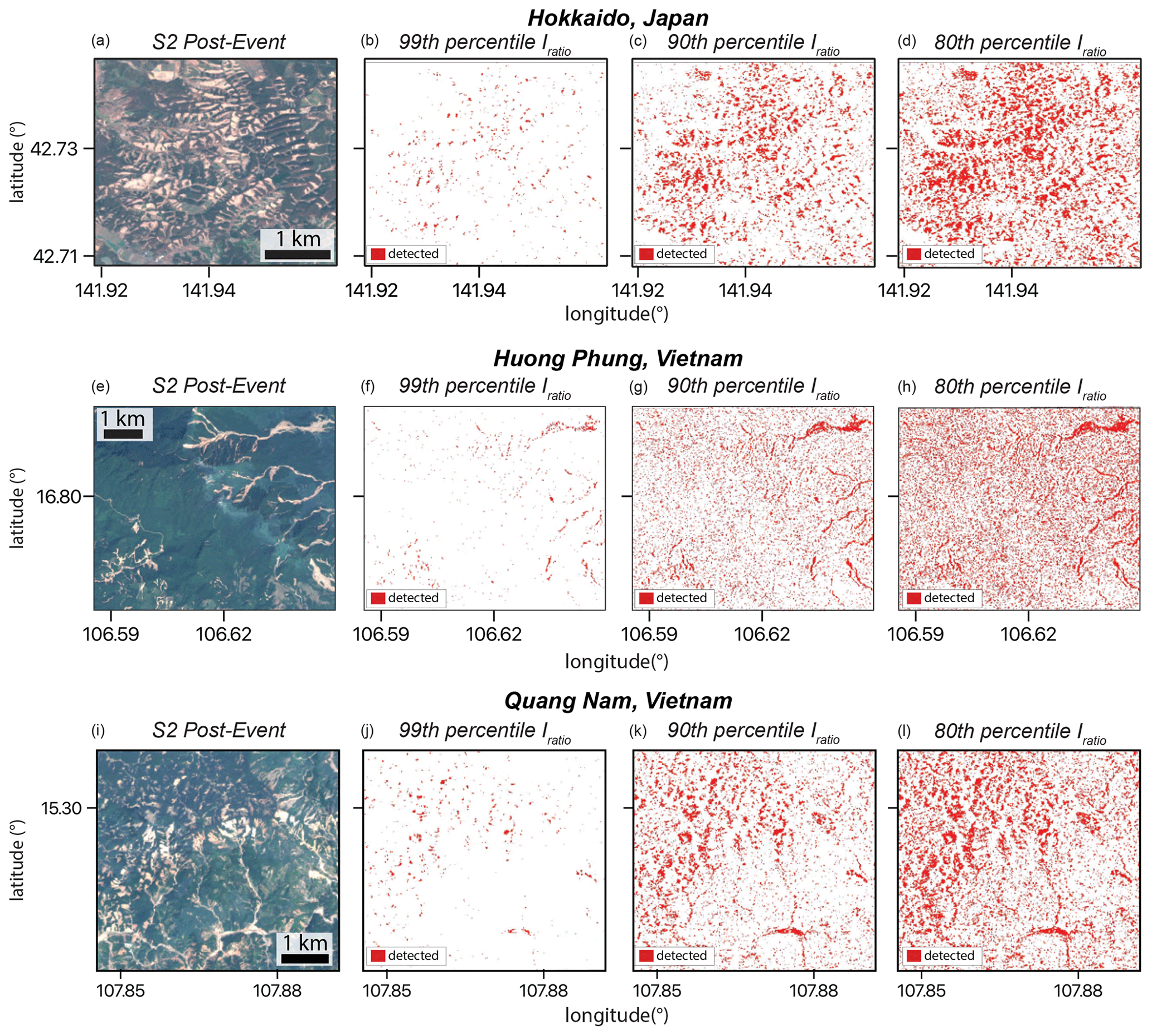
Figure A1 Detected landslides based on I_ratio threshold values (I_TR,H). Sentinel-2 (S2) post-event optical imagery and 99th-, 90th-, and 80th-percentile thresholds for detecting landslides for (a–d) Hokkaidō, Japan; (e–h) Huong Phung, Vietnam; and (i–l) Quang Nam, Vietnam.

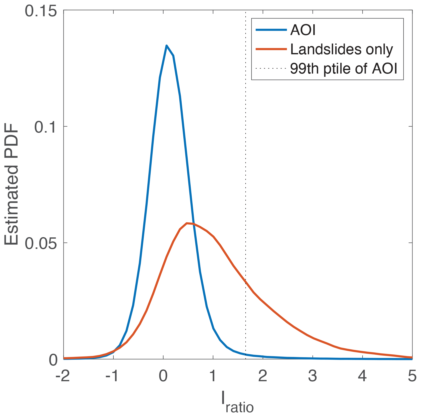
Figure A2 Kernel density function of I_ratio values for the 2018 Hiroshima landslide event. Blue line shows I_ratio distribution for the full AOI including both landslide and non-landslide areas. Red line shows I_ratio distribution for the true landslides mapped by GSI–AJG. I_ratio calculated using combined ascending and descending stacks from 142 pre-event SAR images collected between 1 May 2015 and 29 June 2018 and 133 post-event SAR images collected between 9 July 2018 and 29 May 2020. This plot corresponds to our best-case landslide detection described in Sect. 4.1.