Simulation of tsunami induced by a submarine landslide in a glaciomarine margin: the case of Storfjorden LS-1 (southwestern Svalbard Islands)

A modelling approach to understand the tsunamigenic potentiality of submarine landslides will provide new perspectives on tsunami hazard threat, mostly in polar margins where global climatic change and its related ocean warming may induce future landslides. Here, we use the L-ML-HySEA (Landslide Multilayer Hyperbolic Systems and Efficient Algorithms) numerical model, including wave dispersion, to provide new insights into factors controlling the tsunami characteristics triggered by the Storfjorden LS-1 landslide (southwestern Svalbard). Tsunami waves, determined mainly by the sliding mechanism and the bathymetry, consist of two initial wave dipoles, with troughs to the northeast (Spitsbergen and towards the continent) and crests to the south (seawards) and southwest (Bear Island), reaching more than 3 m of amplitude above the landslide and finally merging into a single wave dipole. The tsunami wave propagation and its coastal impact are governed by the Storfjorden and Kveithola glacial troughs and by the bordering Spitsbergen Bank, which shape the continental shelf. This local bathymetry controls the direction of propagation with a crescent shape front, in plan view, and is responsible for shoaling effects of amplitude values (4.2 m in trough to 4.3 m in crest), amplification (3.7 m in trough to 4 m in crest) and diffraction of the tsunami waves, as well as influencing their coastal impact times.

1 Introduction

Submarine landslides represent one of the most common potential offshore geohazards in the continental slopes of the northern high-latitude margins (Elverhøi et al., 2002; Lee et al., 2009). There, the slope failures are essentially focused at their trough mouth fans (Dowdeswell et al., 2008; Rebesco et al., 2014; Llopart et al., 2016; Ercilla et al., 2022, and references therein). Some landslides may also cause tsunamis, as has been evidenced for the Storegga landslide (3000 km³, at 8.1 kyr), with wave amplitudes of ∼ 20 m at the shore (Bondevik et al., 2003; Haflidason et al., 2005; Kvalstad et al., 2005), or the Hinlopen landslide (1150 km³, at 30 kyr), with wave amplitudes of ∼ 40 m (a.s.l.) (Winkelmann et al., 2008; Vanneste et al., 2006). In the Fram Strait (500 to 1000 km³), located between the main ice retreat areas of Greenland and Svalbard, waves of up to 5.6 m were triggered (Berndt et al., 2009). The factors controlling slope failures in the northern high-latitude margins are still not fully understood. The most common causal factors are the interlayering of underconsolidated glacially derived sediments and low-permeability interglacial hemipelagic clay rich layers, combined with tectonic- and isostatic-related seismicity and/or gas hydrate dissociation (Canals et al., 2004; Kvalstad et al., 2005;Sierro et al., 2009; García et al., 2011; Casas et al., 2013; Vanneste et al., 2014; Moernaut et al., 2017; Llopart et al., 2019).

The understanding of the tsunamigenic potential of submarine landslides still needs to be improved (Chiocci and Ridente, 2011; Løvholt et al., 2020). In this sense back analysis of specific events is commonly used to advance their understanding, as well as to contribute to the hazard assessments of future landslides (Macías et al., 2015; Rodríguez-Morata et al., 2019; Sun and Leslie, 2020). In the European northern high-latitude margins, e.g. Svalbard and Greenland coasts, the tsunami threat has been assessed for a few past landslides. It is important to point out that the tsunami geohazard associated with Holocene landslides such as the Bjørnøyrenna (Laberg and Vorren, 1993), which is the largest landslide (volume of about 1100 km³) in the Barents Sea continental margin; the Nyk landslide in central Norway (Lindberg et al., 2004); or the giant Andøya landslide (northeastern Norwegian–Greenland Sea) (Bugge et al., 1987; Laberg et al., 2000), have not been accurately modelled. The tsunami modelling of recent landslides in this region is important because it will allow us to infer the tsunami potential of future landslides due to climate change and its related ocean warming. Both those interconnected issues are significantly affecting the northern high-latitude margins and may contribute to an increase in the occurrence of submarine landslides, both large and small, in the nearby future, mostly due to gas hydrate dissociation and isostatic-rebound-related earthquakes (Maslin et al., 1998; Tappin, 2010; Urlaub et al., 2013).

Today, the archipelago of Svalbard is one the fastest warming areas of the Arctic Ocean, experiencing an increase in the melting of their glaciers and a rise in the temperature of ocean water circulating along its continental margin (Meleshko et al., 2004; Førland et al., 2013; Skogseth, 2020). This fact may provide adequate conditions to trigger unloading earthquakes and to increase pore water pressure by gas hydrate breakdown, which can destabilize slope sediments (Solheim et al., 2005; Berndt et al., 2009), i.e. the occurrence of landslides and tsunamis in the near future. Both landslides and tsunamis may represent a danger to offshore infrastructures, associated with present and future hydrocarbons exploitation and other renewable energies (Zhang et al., 2019). Tsunamis may also have an impact on the coastal areas of the nearby regions of northwestern Europe, considering the increasing human pressures of these areas (Imamura et al., 2019). The geological record of the Svalbard continental margin can help us to assess the possible tsunamis induced by future landslides. In fact, the sedimentary record of its continental slope evidences numerous landslides, such as the Storfjorden LS-1 landslide, which forms part of the Storfjorden trough mouth fan, and even other recent landslides located in the interfan area of the Storfjorden and Kveithola trough mouth fans (TMFs) (Pedrosa et al., 2011; Rebesco et al., 2012; Lucchi et al., 2012; Llopart et al., 2015).

The relatively medium-size tsunami potential of Storfjorden LS-1 provides new insights into tsunami wave characteristics and evolution. It will help to better understand possible future tsunami hazard in high latitudes. Geomorphic and geotechnical data have been integrated into the L-ML-HySEA (Landslide Multilayer Hyperbolic Systems and Efficient Algorithms) landslide tsunamigenic model simulating landslide dynamics, tsunami wave generation, propagation and coastal impact.

2 Geological setting

Svalbard is located west of the epicontinental Barents Sea and Norwegian continental margin (Fig. 1a). The archipelago resulted from the opening of the northern Atlantic. The major northwest–southeast fault zone is associated with the Knipovich Ridge and the Hornsund Fault Zone (HFZ), crossing the Spitsbergen Island and spreading western of the Barents (Worsley, 1986; Eiken et al., 1994; Engen et al., 2008; Faleide et al., 2008) (Fig. 1b). The post-rift activity of these fault zones has contributed to deforming the Plio-Pleistocene sedimentary sequence (Faleide et al., 1993, 2008; Fiedler and Faleide, 1996). This fault zone has been reactivated by isostatic loading and unloading rebound periods (Pirli et al., 2013; Newton and Huuse, 2017) that are responsible for the local seismicity in the continental margin and can become the trigger of slope failures (Hampel et al., 2009; L'Heureux et al., 2013; Bellwald et al., 2016). Historical earthquakes with magnitudes up to M_w∼ 5 have been recorded (Auriac et al., 2016) (Fig. 1c).

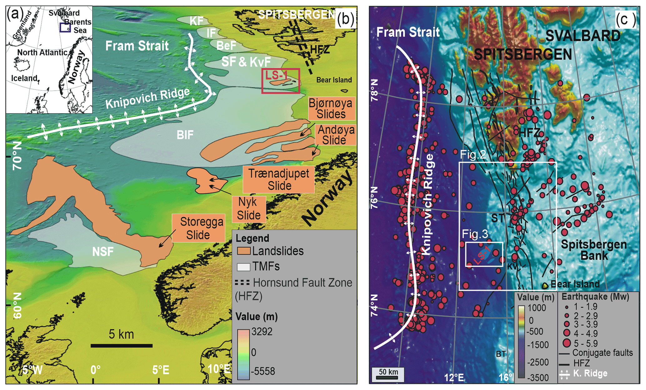
Figure 1 Geographic and geological settings of Storfjorden LS-1. (a) Location map of the study area (blue rectangle). (b) Shaded relief map taken from the International Bathymetric Chart of the Arctic Ocean (IBCAO) version 3.0 (Jakobsson et al., 2012) of the North Atlantic Ocean (Norwegian and Barents seas). The major trough mouth fans (grey polygons) and the major submarine landslides (orange polygons) are located on the map. Compilation from Haflidason et al. (2005), Laberg et al. (2000), Laberg and Vorren (1993), Lindberg et al. (2004), Sejrup et al. (2005), and references therein. KF: Kongsfjorden Fan; IF: Isfjorden Fan; BeF: Bellsund Fan; SF & KvF: Storfjorden Fan and Kveithola Fan; BIF: Bear Island Fan; NSF: North Sea Fan. (c) Shaded relief map of the northwestern Barents Sea (Ottesen et al., 2005) displaying the location of the Hornsund Fault Zone (HFZ) and the historical earthquakes recorded from 1960 to 2018 (source from IRIS catalogue; Incorporated Research Institutions for Seismology). This map also shows the locations of Figs. 2 and 3.

The northwestern Barents continental slope is affected by the Storfjorden and Kveithola TMFs (Fig. 2), created by the high sediment input from the Storfjorden and Kveithola glacial troughs crossing the continental shelf, during the onset of the major Northern Hemisphere glaciations, around 2.6–2.7 Ma (Faleide et al., 1996; Butt et al., 2000; Knies et al., 2009). The Storfjorden TMF seafloor is shaped by the relatively large Storfjorden landslide (LS-1) that extends from the shelf edge to the lower continental slope. In spite of their fresh morphological expression, the seismic stratigraphy indicates that LS-1 (Fig. 3c) is a palaeolandslide above the 0.2 Ma R1 reflector (Rebesco et al., 2012), which is then draped by regional 100 ms (∼ 8 m, considering 1600 m s⁻¹ sediment velocity) thick sediment units (Lucchi et al., 2012; Llopart et al., 2015), and the sliding mass is a subtabular depositional body, between 3 and 5 ms thick (Pedrosa et al., 2011). The high-resolution seismic stratigraphy in the southern Storfjorden TMF is dominated mainly by an alternation of acoustically stratified and transparent units. Eight seismic stratigraphy units (A to G, from top to bottom) have been identified above the R1 reflector (Fig. 3c). Based on acoustic facies they are as follow: the stratified units A, C, E and G and the transparent units B, D and F. The stratified units are usually continuous with high amplitude and draping the existing topography, while the transparent units present an irregular upper boundary and usually a basal erosive surface that describe individual lenses. Comparable seismic facies have also been found in other TMFs (Laberg and Vorren et al., 1993; Cofaigh et al., 2003).

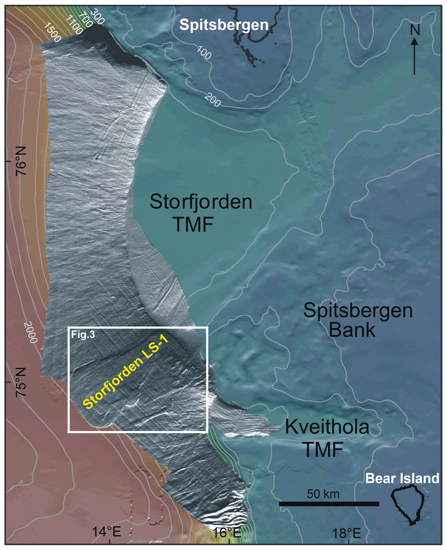
Figure 2 Shaded relief map from merging the regional dataset (colour map, 250 m; Ottesen, 2005) and high-resolution datasets (grey map, 75 m) of the Storfjorden and Kveithola TMFs, where the Storfjorden LS-1 landslide reaches full data coverage.

3 Dataset and methods

3.1 Bathymetric data

For slide modelling, high-resolution multibeam bathymetry datasets from different cruises (SVAIS (The development of an Arctic ice stream-dominated sedimentary system: The southern Svalbard continental margin) onboard BIO (Buque de Investigación Oceanográfica) Hespérides, 2007; EGLACOM (Evolution of a GLacial Arctic COntinental Margin: the southern Svalbard ice stream-dominated sedimentary system) onboard R/V Explora, 2008) have been integrated (Fig. 2). Data processing consisted of cleaning and filtering the navigation data, noise reduction and data editing using the Computer Aided Resource Information System (CARIS) HIPS and SIPS software. Data were gridded at 75 m and partially cover the Storfjorden and Kveithola TMFs (∼ 15 300 km²). The bathymetric mosaic was completed with lower-resolution bathymetry data at 250 m provided by the Norwegian Hydrographic Service (NHS); these were collected between 1965 and 1985 (Ottesen et al., 2005). Moreover, regional gridded bathymetry data for the Arctic Ocean area (IBCAO version 3.0; https://gebco.net, last access: 15 October 2020), interpolated to 2.5 km bin size, were only used for regional figures (Fig. 1b).

Figure 3 Storfjorden and Kveithola interfan TMFs. (a) Shaded relief colour map of the southwestern continental slope of the Storfjorden and Kveithola interfan TMFs. The orange line marks the headwall, and the white lines indicate its sidewalls. The pink line corresponds to the multichannel seismic profile (EG-06) acquired during the EGLACOM cruise. (b) Slope gradient values. Artefacts are induced by the slope parallel to the ship tracks. (c) The top corresponds to the Topographic Parametric Sonar (TOPAS) subbottom profile (modified from Llopart et al., 2015) and multichannel seismic profile (EG-06, modified from Rebesco et al., 2014), acquired during the SVAIS cruise. Both profiles are displayed at the same horizontal and vertical scales to show matching of acoustic facies. The bottom shows the line drawing of the multichannel seismic profile displaying the seismic stratigraphy, where the R1 reflector (in blue) is the base of Storfjorden LS-1 and its top is the unit D (Pedrosa et al., 2011; Rebesco et al., 2014; Llopart et al., 2015). TWTT: two-way travel time. (d) Table with the seismic units and subunits, ages, and their lithologies (modified from Llopart et al., 2015).

3.2 Tsunami numerical modelling

The L-ML-HySEA is a mathematical model, which implements a two-phase model to reproduce the interaction between the landslide granular material and the fluid. In the present work, a multilayer non-hydrostatic shallow-water model is considered in order to model the evolution of the ambient water, taking into account dispersive water waves (Fernández-Nieto et al., 2018), and to simulate the kinematics of the Storfjorden LS-1 landslide using the Savage–Hutter model (Eq. 3) (Fernando-Nieto et al., 2008).

The L-ML-HySEA model was validated using laboratory experimental data for landslide-generated tsunamis. A milestone in the validation process of this code consisted in the numerical simulation of the Lituya Bay 1958 mega tsunami with real topobathymetric data obtained from González-Vida et al. (2019). The simulation was also used to generate initial conditions for the Method of Splitting Tsunami (MOST), in order to be initialized for the landslide-generated tsunami scenarios of the National Tsunami Hazard Mitigation Program (NTHMP) mandatory benchmarks in the USA (EDANYA Research Group, HySEA; results for NTHMP's tsunami benchmarking process for landslide-generated tsunamis are available at https://edanya.uma.es/hysea/index.php/benchmarks/landslide-generated, last access: 1 January 2015).

L-ML-HySEA needs to incorporate the physical properties of the sediment involved in the landslides. In the Storfjorden (LS-1) case, properties determined by Lucchi et al. (2013) and Llopart et al. (2019) were used. For the purpose of modelling, we have assumed that the landslide took place in a single event. The simulation has been performed by considering a ∼ 1.3^∘ critical slope repose angle, since that value has given the best results across the models.

3.2.1 Reconstruction of pre-landslide bathymetry and landslide body geometry

To perform the L-ML-HySEA numerical simulation, it is necessary to reconstruct the pre-bathymetry before the seafloor failure (Macías et al., 2015). For this aim, we used the high-resolution multibeam bathymetry together with seismic profiles published to define the landslide location, its body geometry and its buried thickness (Pedrosa et al., 2011; Lucchi et al., 2012; Rebesco et al., 2012, 2014; Llopart 2015). We assume that the sedimentary infill thickness of 100 ms (Llopart et al., 2015) is roughly similar inside and outside of the landslide and then the present-day bathymetry reproduces the pre-Storfjorden LS-1 100 ms difference.

The pre-Storfjorden LS-1 landslide (Fig. 4a) has been calculated by filling the current headwall and lateral-scarp areas using the cartographic sewing technique on the bathymetry with B splines (Lee et al., 1997) and defining a network of B-spline patches (Eck and Hoppe, 1996). The corresponding control vertices splines were developed using CAD (computer-aided design) software tools through contour lines from the DEM (digital elevation model) and defined by a tolerance rectangle. When creating the spline, the tolerance rectangle is displayed in the form of construction lines. The control vertices of the rectangle, which are shown as circles, influence the spline curves. The spline is tangent to the tolerance rectangle at the start and end points. In this way, the curve ends up adapting to the hypothetical geometry that best fits each patch. Once the splines were developed, patches were densified through the existing DEM and the points were calculated through the splines, generating a new complete DEM without patches. This procedure uses only data points that are not affected by the landslide and assumes convergence of both datasets (boundary conditions) where the slide scars terminate. A second step involves obtaining the volume of the slid sediment body (Fig. 4b) by calculating the difference between the reconstructed pre- and post-landslide bathymetry.

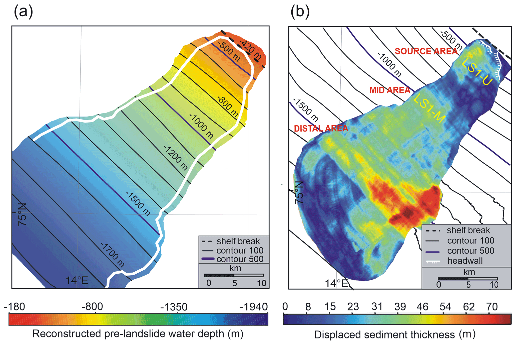
Figure 4 The Storfjorden LS-1 landslide geometry. (a) Reconstruction of pre-landslide seafloor morphology. (b) Available displaced sediment thickness in metres. Note the location of the different sliding upper and middle sectors (LS1-U and LS1-M, respectively).

3.2.2 The L-ML-HySEA model equations and discretization

The Multilayer-HySEA model consists of a two-phase model that represents the interaction between a submarine or subaerial landslide (composed by granular material) and the ambient fluid. A multilayer non-hydrostatic shallow-water model is considered for modelling the evolution of the ambient water, and for simulating the kinematics of the submarine/subaerial landslide the Savage–Hutter model is used. As can be found in Fernández-Nieto et al. (2018) the simplest model that can be used for this purpose consists of a single fluid layer (Eq. 1) modelled by a non-hydrostatic shallow-water equation coupled with a Savage–Hutter model (Eq. 2).

$$\begin{array}{}\text{(1)}& {\displaystyle }\text{S-W system}\left\{\begin{array}{l}{\partial }_{t}h+{\partial }_x\left(hu\right)=\mathrm{0},\\ {\partial }_t\left(hu\right)+{\partial }_x\left(h{u}^{\mathrm{2}}+\frac{\mathrm{1}}{\mathrm{2}}g{h}^{\mathrm{2}}\right)\\ -gh{\partial }_x\left(H-z_s\right)=n_a\left(u_s-u\right),\end{array}\right.\text{(2)}& {\displaystyle }\text{S-H system}\left\{\begin{array}{l}{\partial }_t{z}_s+{\partial }_x\left(z_s{u}_s\right)=\mathrm{0},\\ {\partial }_t\left(z_s{u}_s\right)+{\partial }_x\left(z_s{u}_s^{\mathrm{2}}+\frac{\mathrm{1}}{\mathrm{2}}g\left(\mathrm{1}-r\right)z_s^{\mathrm{2}}\right)\\ -g\left(\mathrm{1}-r\right)z_s{\partial }_{x}H=-r{n}_a\left(u_s-u\right)+{\mathit{\tau }}_P,\end{array}\right.\end{array}$$

where g is the gravity acceleration (g=9.81 m s⁻²); H(x) is the non-erodible bathymetry measured from a predetermined reference level, z_s(x,t) denotes the thickness of the layer of granular material at each point x at time t, h(x,t) is the total water depth, and η(x,t) represents the free surface (measured from the same aforementioned fixed reference level) and is given by $\mathit{\eta }=h+z_s-H$. u(x,t) and u_s(x,t) are the averaged horizontal velocity for the water and for the granular material, respectively, and $r=\frac{{\mathit{\rho }}_{\mathrm{1}}}{{\mathit{\rho }}_{\mathrm{2}}}$ is the ratio of densities between the ambient fluid and the granular material. The friction between the fluid and the granular layer is parameterized with the term n_a(u_s−u). Finally, τ_P(x,t) represents the friction between the granular slide and the non-erodible bottom surface. The parameterization follows the system proposed in Pouliquen and Forterre (2002).

These two models are coupled through the boundary conditions at their interface. The parameter r represents the ratio of densities between the ambient fluid and the granular material (slide liquefaction parameter).

Usually, it is formulated that

$$\begin{array}{}\text{(3)}& r={\displaystyle \frac{{\mathit{\rho }}_{\mathrm{f}}}{{\mathit{\rho }}_b}},{\mathit{\rho }}_b=\left(\mathrm{1}-\mathit{\phi }\right){\mathit{\rho }}_s+\mathit{\phi }{\mathit{\rho }}_{\mathrm{f}},\end{array}$$

where ρ_s represents the typical density of the granular material and ρ_f is the density of the fluid (ρ_s>ρ_f), both considered constant, and φ represents the porosity ($\mathrm{0}\le \mathit{\phi }<\mathrm{1}$). In this model φ is supposed to be constant in space and time, and, consequently, the ratio r is also constant. This ratio r ranges from 0 to 1 (i.e. $\mathrm{0}<r<\mathrm{1})$ and is a value difficult to estimate even in a uniform material, as it depends on the porosity (and ρ_f and ρ_s are also assumed constant) (Fig. 5).

Nevertheless, this system is not accurate enough for modelling landslides where the dispersive effects are relevant, so the model to be considered in this work and described in the next section is the L-ML-HySEA.

Figure 5 Schematic figure to describe the multilayer system, with water height (h), unchanged non-erodible bathymetry (H), depth-averaged velocity in the x direction (μ_α), depth-averaged velocity in the z direction (ω_α), sediment thickness (z_s), non-hydrostatic pressure at the interface ($P\mathit{\alpha }-\mathrm{1}/\mathrm{2}$), free-surface elevation measured from a fixed reference level (η) and the number of layers (L).

The fluid model

The ambient fluid is modelled by a multilayer non-hydrostatic shallow-water system (Férnandez-Nieto et al., 2018) so that dispersive water waves can be taken into account. The model is obtained by a process of depth averaging of the Euler equations and can be interpreted as a semi-discretization with respect to the vertical coordinate.

The total pressure is decomposed into the sum of hydrostatic and non-hydrostatic components, in order to take into account dispersive effects. In this process, the horizontal and vertical velocities are supposed to have constant vertical profiles. The resulting multilayer model admits an exact energy balance, and when the number of layers increases, the linear dispersion relation of the linear model converges to the same of Airy's theory. Finally, the model proposed in Férnandez-Nieto et al. (2018) can be written in a compact form as

$$\begin{array}{}\text{(4)}& \left\{\begin{array}{l}{\partial }_{t}h+{\partial }_x\left(hu\right)=\mathrm{0},\\ {\partial }_t\left(h{u}_{\mathit{\alpha }}\right)+{\partial }_x\left(h{u}_{\mathit{\alpha }}^{\mathrm{2}}+\frac{\mathrm{1}}{\mathrm{2}}g{h}^{\mathrm{2}}\right)-gh{\partial }_x\left(H-z_s\right)\\ +u_{\mathit{\alpha }+\frac{\mathrm{1}}{\mathrm{2}}}{\mathrm{\Gamma }}_{\mathit{\alpha }+\frac{\mathrm{1}}{\mathrm{2}}}-u_{\mathit{\alpha }-\frac{\mathrm{1}}{\mathrm{2}}}{\mathrm{\Gamma }}_{\mathit{\alpha }-\frac{\mathrm{1}}{\mathrm{2}}}=-h\left({\partial }_x{p}_{\mathit{\alpha }}+{\mathit{\sigma }}_{\mathit{\alpha }}{\partial }_z{p}_{\mathit{\alpha }}\right)-{\mathit{\tau }}_{\mathit{\alpha }},\\ {\partial }_t\left(h{w}_{\mathit{\alpha }}\right)+{\partial }_x\left(h{u}_{\mathit{\alpha }}{w}_{\mathit{\alpha }}\right)+w_{\mathit{\alpha }+\frac{\mathrm{1}}{\mathrm{2}}}{\mathrm{\Gamma }}_{\mathit{\alpha }+\frac{\mathrm{1}}{\mathrm{2}}}\\ -w_{\mathit{\alpha }-\frac{\mathrm{1}}{\mathrm{2}}}{\mathrm{\Gamma }}_{\mathit{\alpha }-\frac{\mathrm{1}}{\mathrm{2}}}=-h{\partial }_z{p}_{\mathit{\alpha }},\\ {\partial }_x{u}_{\mathit{\alpha }-\frac{\mathrm{1}}{\mathrm{2}}}+{\mathit{\sigma }}_{\mathit{\alpha }-\frac{\mathrm{1}}{\mathrm{2}}}{\partial }_z{u}_{\mathit{\alpha }-\frac{\mathrm{1}}{\mathrm{2}}}+{\partial }_z{w}_{\mathit{\alpha }-\frac{\mathrm{1}}{\mathrm{2}}}=\mathrm{0},\end{array}\right.\end{array}$$

for $\mathit{\alpha }\in \mathit{\{}\mathrm{1},\mathrm{2},\mathrm{\dots },L\mathit{\}}$, with L being the number of layers and where the following notation has been used:

$$f_{\mathit{\alpha }+\mathrm{1}/\mathrm{2}}={\displaystyle \frac{\mathrm{1}}{\mathrm{2}}}\left(f_{\mathit{\alpha }+\mathrm{1}}+f_{\mathit{\alpha }}\right){\partial }_z{f}_{\mathit{\alpha }+\mathrm{1}/\mathrm{2}}={\displaystyle \frac{\mathrm{1}}{h\mathrm{\Delta }s}}\left(f_{\mathit{\alpha }+\mathrm{1}}-f_{\mathit{\alpha }}\right),$$

where f denotes one of the generic variables of the system (i.e. u_α, w_α and p_α), $\mathrm{\Delta }s=\mathrm{1}/L$ and

$$\begin{array}{ll}{\displaystyle }{\mathit{\sigma }}_{\mathit{\alpha }}& {\displaystyle }={\partial }_x\left(H-z_s-h\mathrm{\Delta }s\left(\mathit{\alpha }-\mathrm{1}/\mathrm{2}\right)\right){\mathit{\sigma }}_{\mathit{\alpha }-\mathrm{1}/\mathrm{2}}\\ {\displaystyle }& {\displaystyle }={\partial }_x\left(H-z_s-h\mathrm{\Delta }s\left(\mathit{\alpha }-\mathrm{1}\right)\right).\end{array}$$

A schematic picture of model configuration is where the total water height h is decomposed along the vertical axis into L≥1 layers (Fig. 5). The depth-averaged velocities in the x and z directions are written as u_α and w_α, respectively. The non-hydrostatic pressure at the interface $z_{\mathit{\alpha }+\mathrm{1}/\mathrm{2}}$ is denoted by $p_{\mathit{\alpha }+\mathrm{1}/\mathrm{2}}$. The free-surface elevation measured from a fixed reference level (for example the still-water level or mean level in the ocean) is written as η and $\mathit{\eta }=h-H+z_s$, where again H(x) is the unchanged non-erodible bathymetry measured from the same fixed reference level. τ_α=0, for α>1 and τ₁ is given by

$${\mathit{\tau }}_{\mathrm{1}}={\mathit{\tau }}_{\mathrm{b}}-n_a\left(u_s-u_{\mathrm{1}}\right),$$

where τ_b stands for a classical Manning-type parameterization for the bottom shear stress and, in this model, is given by

$${\mathit{\tau }}_{\mathrm{b}}=gh{\displaystyle \frac{n^{\mathrm{2}}}{h^{\mathrm{4}/\mathrm{3}}}}{u}_{\mathrm{1}}\left|u_{\mathrm{1}}\right|,$$

and n_a(u_s−u₁) accounts for the friction between the fluid and the granular layer. The latest two terms are only present at the lowest layer (α=1). Finally, for $\mathit{\alpha }=\mathrm{1},\mathrm{\dots },L-\mathrm{1}$, ${\mathrm{\Gamma }}_{\mathit{\alpha }+\mathrm{1}/\mathrm{2}}$ parameterizes the mass transfer across interfaces, and those terms are defined by

$${\mathrm{\Gamma }}_{\mathit{\alpha }+\mathrm{1}/\mathrm{2}}={\sum }_{\mathit{\beta }=\mathit{\alpha }+\mathrm{1}}^L{\partial }_x\left(h\mathrm{\Delta }s\left(u_{\mathit{\beta }}-\stackrel{\mathrm{‾}}{u}\right)\right),\stackrel{\mathrm{‾}}{u}={\sum }_{\mathit{\alpha }=\mathrm{1}}^L\mathrm{\Delta }s{u}_{\mathit{\alpha }}.$$

Here, we suppose that ${\mathrm{\Gamma }}_{\mathrm{1}/\mathrm{2}}={\mathrm{\Gamma }}_{L+\mathrm{1}/\mathrm{2}}=\mathrm{0}$, which means that there is no mass transfer through the seafloor or the water free surface. To close the system, the boundary condition

$$p_{L+\mathrm{1}/\mathrm{2}}=\mathrm{0}$$

is imposed at the free surface, and the boundary conditions

$$u_{\mathrm{0}}=\mathrm{0},w_{\mathrm{0}}=-{\partial }_t\left(H-z_s\right)$$

are imposed at the bottom. The last two conditions enter into the incompressibility relation for the lowest layer (α=1), given by

$${\partial }_x{u}_{\mathrm{1}/\mathrm{2}}+{\mathit{\sigma }}_{\mathrm{1}/\mathrm{2}}{\partial }_z{u}_{\mathrm{1}/\mathrm{2}}+{\partial }_z{w}_{\mathrm{1}/\mathrm{2}}=\mathrm{0}.$$

It should be noted that the hydrodynamic model described here and the morphodynamic model described in the next subsection are coupled through the unknown z_s, which, in the case of the model described here, is present in the equations and in the boundary condition ($w_{\mathrm{0}}=-{\partial }_t\left(H-z_s\right))$.

Some dispersive properties of the system (4) were originally studied in (Férnandez-Nieto et al., 2018). Moreover, for a better-detailed study on the dispersion relation (such as “phase velocity”, “group velocity” and “linear shoaling”) the reader is referred to the work of Macías et al. (2020).

Along the derivation of the hydrodynamic model presented here, the rigid-lid assumption for the free surface of the ambient fluid was adopted. Therefore, pressure variations induced by the fluctuation on the free surface of the ambient fluid over the landslide are neglected.

The landslide model

The 1D Savage–Hutter method implemented in the model is given by system (2). The friction law τ_P (Pouliquen and Forterre, 2002) is given by the expression

$${\mathit{\tau }}_P=-g\left(\mathrm{1}-r\right)\mathit{\mu }{z}_s{\displaystyle \frac{u_s}{\left|u_s\right|}},$$

where μ is a constant friction coefficient with a fundamental role because it controls the movement of the landslide. Usually, μ is given by the Coulomb friction law as it is the simplest parameterization that can be used in landslide models. However, it is well known that a constant friction coefficient does not allow for models to reproduce the steady uniform flows over rough beds that are observed in the laboratory for a range of inclination angles. In the work of Pouliquen and Forterre (2002), in order to reproduce these flows, the authors introduced an empirical friction coefficient μ that depends on the norm of the mean velocity u_s on the thickness z_s of the granular layer and on the Froude number $\mathit{Fr}=\frac{u_s}{\sqrt{g{z}_s}}$. The friction law is given by

$$\mathit{\mu }\left(z_s,u_s\right)=\left\{\begin{array}{ll}{\mathit{\mu }}_{\mathrm{start}}\left(z_s\right)+{\left(\frac{\mathit{Fr}}{\mathit{\beta }}\right)}^{\mathit{\gamma }},& \mathrm{for}\mathit{Fr}<\mathit{\beta },\\ \left({\mathit{\mu }}_{\mathrm{stop}}\left(z_s\right)-{\mathit{\mu }}_{\mathrm{start}}\left(z_s\right)\right)& \\ {\mathit{\mu }}_{\mathrm{stop}}\left(z_s\right),& \mathrm{for}\mathit{\beta }\le \mathit{Fr},\end{array}\right.$$

with

$$\begin{array}{ll}{\displaystyle }& {\displaystyle }{\mathit{\mu }}_{\mathrm{start}}\left(z_s\right)=\tan \left({\mathit{\delta }}_{\mathrm{3}}\right)+\left(\tan \left({\mathit{\delta }}_{\mathrm{2}}\right)-\tan \left({\mathit{\delta }}_{\mathrm{1}}\right)\right)\exp \left({\displaystyle \frac{-z_s}{d_{\mathrm{s}}}}\right),\\ {\displaystyle }& {\displaystyle }{\mathit{\mu }}_{\mathrm{stop}}\left(z_s\right)=\tan \left({\mathit{\delta }}_{\mathrm{1}}\right)+\left(\tan \left({\mathit{\delta }}_{\mathrm{2}}\right)-\tan \left({\mathit{\delta }}_{\mathrm{1}}\right)\right)\exp \left({\displaystyle \frac{-z_s\mathit{\beta }}{d_{\mathrm{s}}\mathit{Fr}}}\right),\end{array}$$

where d_s represents the mean size of the grains. β=0.136 and $\mathit{\gamma }={\mathrm{10}}^{-\mathrm{3}}$ are empirical parameters. tan (δ₁) and tan (δ₂) are the characteristic angles of the material, and tan (δ₃) is another friction angle related to the behaviour when starting from rest. This law has been widely used in the literature (see for instance Brunet et al., 2017).

It is important to remark that this slide model can also be adapted to simulate subaerial landslides. The presence of the term (1−r), in the definition of the Pouliquen–Forterre friction law, is due to the buoyancy effects, which must be taken into account only in the case that the granular material layer is submerged in the fluid. Otherwise, this term must be replaced by 1 in order to consider subaerial landslides.

In Macías et al. (2021) the reader can find the details about the numerical algorithms used to implement the model.

The discretization of the resulting systems is difficult. For the hydrostatic systems that are expressed as non-conservative hyperbolic systems, the natural extension of the numerical schemes proposed in Escalante et al. (2018, 2019) has been adopted and then solved using a second-order HLL (Harten–Lax–van Leer), positive-preserving, well-balanced, path-conservative finite-volume numerical scheme (see Castro Díaz and Fernandez-Nieto, 2012). Then, the non-hydrostatic pressure corrections at the vertical interfaces required the discretization of an elliptic operator, and that was done using standard second-order central finite differences. This resulted in a linear system that was solved using an iterative scheduled Jacobi method. Finally, the computed non-hydrostatic corrections were used to update the horizontal and vertical momentum equations at each layer, and, at the same time, the frictions were also discretized (see Escalante et al., 2018, 2019). For the discretization of the Coulomb friction term, the procedures presented in Fernández-Nieto et al. (2008) were followed.

The resulting 2D numerical scheme is well balanced for the water at rest stationary solution and is L^∞ stable under the normal CFL (Courant–Friedrichs–Lewy) condition. The scheme is also positive preserving; that means that the thickness of the water layer will be always positive or zero but never negative and can be used with emerging topographies.

For dealing with numerical experiments in 2D regions, the computational domain must be decomposed into cells or finite volumes with a simple geometry. Here, a Cartesian-type UTM (Universal Transverse Mercator) was used. The 2D numerical algorithm for the hydrodynamic hyperbolic component of the coupled system is well suited to be parallelized and implemented in GPU (graphics processing unit) architectures, as is shown in Castro et al. (2011). Unfortunately, the standard treatment of the elliptic part of the system is not compatible with the parallelization of the algorithms. However, in Escalante et al. (2018, 2019), a multi-GPU implementation was presented and made possible because of the compactness of the numerical stencil and the massive parallelization of the Jacobi method. Such a multi-GPU implementation of the complete algorithm results in much shorter computational times, and that is the reason why it was used in this work.

4 Results

4.1 The Storfjorden LS-1 landslide geometry

The Storfjorden LS-1 landslide is ∼ 60 km in length and covers an area of more than 1300 km² (Llopart et al., 2015). Three main morphological elements are imaged by the multibeam bathymetry: the headwall, sidewalls and sliding area (Fig. 3a). The headwall displays a well-defined seaward-concave scarp that forms an amphitheatre-like feature about 12 km long and > 50 m in relief. Its slide scar is incised into the shelf edge at 420–480 m water depth. The northwestern sidewall is defined by a striking 25 km long scarp, 35–40 m in relief, with a rectilinear to slightly sinuous pathway. The southeastern sidewall is 35 km long with 25 to 80 m of relief, representing the highest in the mid area (∼ 1500 m water depth). The width between the sidewalls is variable downslope. The sidewalls are roughly parallel and define a bottleneck shape of 18 km wide, down at ∼ 1330 m water depth, which increases to 32 km at ∼ 1900 m water depth. The sliding area displays an elongated lobate shape, in plan view, with an irregular seafloor. The seafloor gradients are typically 2 to 3^∘ at ∼ 1330 m water depth and < 2^∘ toward the distal ends (Fig. 3b). The chaotic landslide deposits in the upper slope (800 m depth) are shown in Fig. 3c (Llopart et al., 2015).

4.2 Submarine landslide and tsunami numerical simulations

The numerical simulation consists of several successive steps aimed at reconstructing (i) the smooth pre-landslide upper slope and landslide body geometry following the methods described in Sect. 3.2.1 (Fig. 4), (ii) the landslide dynamic (Fig. 6), (iii) the tsunami wave generation (Fig. 7), and (iv) the tsunami wave propagation and its impacts on the coast (Figs. 8 and 9).

4.2.1 Modelling the landslide dynamic

Once the smooth pre-landslide upper slope had been calculated, following the methods described in Sect. 3.2.1 (Fig. 4), the landslide body geometry was determined. The numerical landslide rupture simulation begins with the slope failure of Storfjorden LS-1, which assumes that it fails at once and moves downslope by gravitational forces (Macías et al., 2015). Conventional studies about submarine slides show the difficulty in assessing whether their occurrence represents unique events (Casas et al., 2016; Chiocci and Casalbore, 2017; Vázquez et al., 2022). The morphological results would also support that assumption for Storfjorden LS-1, due to the lack of retrogressive structures, which would point to a decrease in the tsunamigenic potential (Harbitz et al., 2006). A few local and small-scale slope failures seem to occur on the southeastern flank in the mid slope (∼ 1600 m deep), but they would not be significant in the modelling of the main landslide event, due to its low potential to transfer deformation to the water column.

In addition, by comparison with similar deposits from other continental slopes (Iglesias et al., 2012; Casas et al., 2013; Casas et al., 2013; Vanneste et al., 2006; Winkelmann et al., 2008), Storfjorden LS-1 shows a well-defined arcuate slide scar, mostly rectilinear side walls and a cutting basal shear surface. Its moving mass defines a subtabular body with chaotic deposits and without apparent internal discontinuities that sharply interrupt the lateral continuity of the surrounding deposits (Pedrosa et al., 2011; Lucchi et al., 2012). All these characteristics put together tentatively point to a single sliding process, not being demonstrated as multiple failures in the previous literature (Pedrosa et al., 2011; Lucchi et al., 2012; Rebesco et al., 2012, 2013). The difference between pre- and post-landslide bathymetries is 40 km³, a volume between 33 km³ proposed by Pedrosa et al. (2011) and 46 km³ by Llopart et al. (2015). The numerical landslide rupture simulation shows that the moving mass was comprised of two domains with different behaviour, based on the velocity pattern (Fig. 6a and b). At 1 min after the slide, an upper-slope domain (LS1-U, ∼ 500 m water depth, ∼ 3^∘ slope gradients) is related to the moving sediment nearest to the slide scar and moves faster (v_u=5 m s⁻¹) than the mid-slope domain (LS1-M, ∼ 1000 m water depth, 2^∘ slope gradients, v_m=1 m s⁻¹) (Fig. 6a, step 1; Fig. 7, step 1; Supplement video 1, EDANYA Research Group, 2022a). At 4 min, the velocity increases in the upper-slope domain as v_u= 30 m s⁻¹ and in the mid-slope domain as v_m=22 m s⁻¹ (Fig. 6, step 2; Fig. 7, step 2; Supplement video 1). At 20 min, the sliding velocity maximum in the frontal area is v_f= 20 m s⁻¹ and decreases gradually towards the sides of the slide with values around v_s= 15 m s⁻¹ (Fig. 6c, step 10; Fig. 7, step 10; Supplement video 1). At 25 min, the sediment sliding became homogeneous in the distal area (∼ 1500 m water depth). The velocity decreases gradually downslope, where the frontal area of sediment sliding velocities reach around v_f= 10 m s⁻¹ and in distal area v_s= 2–5 m s⁻¹.

The landslide characteristics modelled by L-ML-HySEA determine an average velocity (v_a) of 25 m s⁻¹, a terminal time (t_t) of ∼ 40 min and a characteristic distance (d_c) of at least ∼ 60 km.

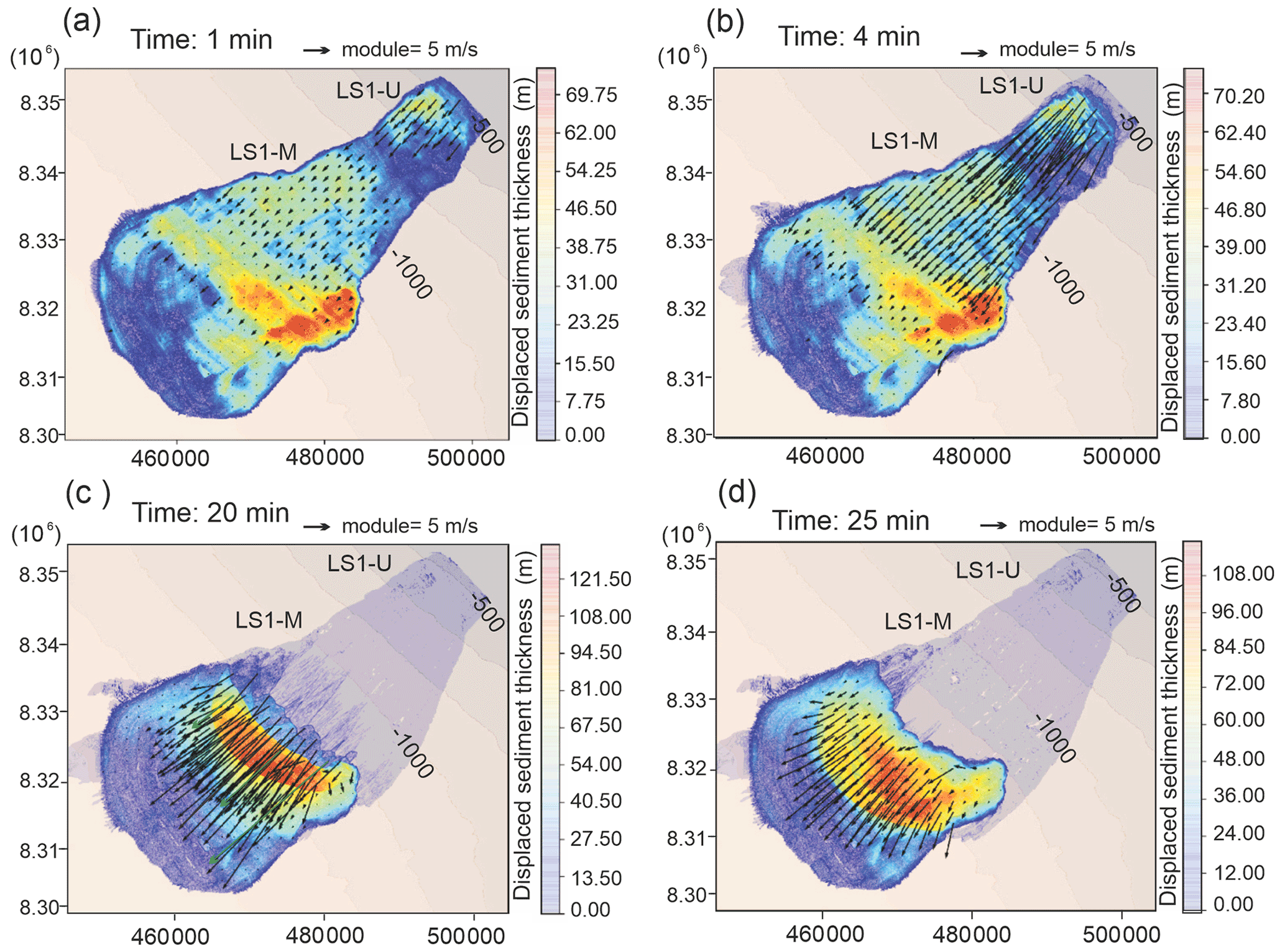
Figure 6 Velocity pattern of the landslide in different frames and the displaced sediment thickness. (a) A 1 min frame, where the upper-slope domain (LS1-U, ∼ 500 m water depth, 3^∘ slope gradient) with an average velocity v_u= 5 m s⁻¹ contrasts with the mid-slope domain (LS1-M, ∼ 1000 m water depth; 2^∘ slope gradients) with an average velocity v_m= 1 m s⁻¹. (b) A 4 min frame, with a progressive velocity increase in both areas (v_u= 30 m s⁻¹ and v_m= 22 m s⁻¹, respectively). (c) A 20 min frame, where velocity is maximum in the frontal area as v_f= 20 m s⁻¹, coinciding with maximum sediment thickness displacement (122–108 m) and decrease towards the sides as v_s= 15 m s⁻¹. (d) A 25 min frame, where both moving masses are joined with central velocity v_f= 10 m s⁻¹ and lateral velocity v_s= 2–5 m s⁻¹ in the distal area (∼ 1500 m water depth).

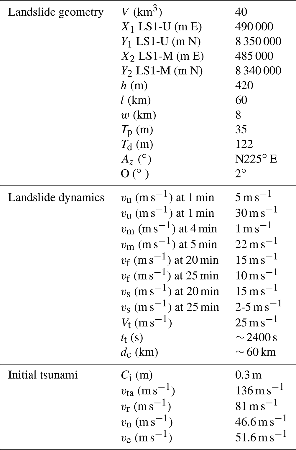
Table 1 Storfjorden LS-1 geometry and mechanical characteristics. The inputs for the model are related to the landslide geometry: the total volume (V), the longitude and latitude of the submarine landslide relative to the LS1-U slope area (X₁, Y₁) and the LS1-M slope area (X₂, Y₂), the initial depth (h) before the slope failure, the length (l) (long axis) and width (w) (small axis), the maximum thickness in the proximal and distal areas (T_p and T_d, respectively), the mean azimuth direction of the landslide (A_z), and the mean slope gradient (O). The outputs of the model are related to the landslide dynamic: velocities to the landslide in the upper slope (v_u) and the landslide located in the mid slope (v_m), sliding sediment in the frontal area (v_f), sliding sediment in the sides (v_d), total velocity (V_t), terminal duration (t_t), and characteristic distance (d_c). The outputs related to initial tsunamis: wave crest (C_i) tsunami velocity at 1900 m depth (v_ts), tsunami wave velocity during refraction (v_r), tsunami wave velocity toward the north (v_n) and tsunami wave velocity toward the southeast (v_e). LS1-U: Storfjorden landslide upper slope; LS1-M: Storfjorden landslide mid slope.

4.2.2 Tsunami wave generation

Free-water-surface changes at any point along the time are determined according to seafloor deformation (Fig. 7 and Supplement video 1). In the initial stage (4 to 5 min), the tsunami wave has two northwest–southeast-trending dipoles, LS1-U, smaller (25 km long) and more striking, and LS1-M, larger (35 km long) and smoother. They have been created by the water mass infilling the empty spaces produced by the sudden evacuations and uplifting of fast-downslope-moving mass. Both wave dipoles have the troughs in shallower waters (∼ 600 to 800 m) than their respective crests (∼ 700 to 1000 m water depth) (Fig. 7, steps 1 and 8). The synthetic marigram on the upper slope (station 1) of Storfjorden LS-1 (Fig. 9a, b and c) highlights the initial wave generation with the crest and trough well defined, registering a crest amplitude value of 0.4 m (above LS1-U) and a trough amplitude value of up to 1.1 m at 3 min, followed by a crest amplitude value of 0.3 m (Fig. 8, step 1; Fig. 9b; Supplement video 2, EDANYA Research Group, 2022b).

After 3 min, the two initial dipoles evolve into a single northwest–southeast-trending dipole (crest amplitude value of 0.3 m), whose trough (0.5 m) is also in shallower waters than the crest (Fig. 7, step 3; Fig. 8, step 1). Wave rebound occurs (Fig. 7, steps 4 to 9) when a maximum amplitude of ∼ 2.7 m is registered over the distal area of the landslide (Fig. 9c, station 2; Supplement video 2). At 7 to 9 min, a new crest wave amplitude value of 0.5 m appears parallel to the single dipole (Fig. 7, steps 4 to 5; Supplement video 1) in shallower waters. It enlarges with time up to 0.7 m, whereas the trough largely keeps its dimensions or relief. At the 16 min mark, the tsunami wave reaches the highest amplitude (at 1780 m water depth), with a trough amplitude value of 2 m and a crest amplitude value of 0.7 m (Fig. 9, station 2).

Figure 7 Main composition in 12 consecutive frames. (a) Evolution of the landslide, where two sliding sediment masses in the firsts 25 min can be distinguished, one in the upper slope (LS1-U) and the other one in the mid slope (LS1-M), which are merged into a unique one after 25 min. The colour scale corresponds to available sediment thickness to be displaced in metres. (b) Dipole wave evolution of the outgoing tsunami with the wave height values.

At 25 min, the tsunami wave evolves into a larger dipole above the landslide, opposite to the first ones, with a trough amplitude value of 0.5 m and a crest amplitude value of 0.3 m (at 1200 m water depth). This dipole gets smaller with time, with a crest amplitude value of 0.5 m in shallower waters (900 m water depth) covering large areas with time (Fig. 7, step 10).

4.2.3 Tsunami wave propagation and coastal impact

The tsunami wave dynamics are illustrated by the maps of the wave height across time (Fig. 8 and Supplement videos 1 and 2). Synthetic marigrams have been included at key locations in order to highlight the wave propagation and coastal impact in the northwestern flank of Spitsbergen Bank (Fig. 9d, station 3), the onshore area of the Kveithola glacial trough (Fig. 9e, station 4), Spitsbergen Bank (Fig. 9f, station 5), the onshore northern boundary of the mid shelf of Storfjorden glacial trough (Fig. 9g, station 7) and the onshore southwestern Spitsbergen coast (Fig. 9h and i, stations 7 to 8).

The initial tsunami wave starts propagating from the landslide area with a trough wave moving northeast towards the coast and a crest wave moving southwest (Fig. 8, step 3; Supplement videos 1 and 2). The tsunami waves propagate elliptically, with the crest and trough elongated in the northwest–southeast direction (Fig. 7, step 3) and a total velocity (v_ts) of ∼ 136 m s⁻¹. During the tsunami propagation from depth (∼ 1900 m) towards shallow water (∼ 250 m) (Fig. 8 and Supplement video 2), the refraction phenomenon occurs during shoaling. The synthetic marigram records the refraction clearly due to an irregular variation in the general amplitude pattern (Fig. 9d, station 3). Refraction effects in a wave front show a decrease in velocity down to v_r= 81 m s⁻¹ and an increase in amplitude. The values change from a trough amplitude of 0.25 m to a crest amplitude value of 0.18 m (Fig. 9e, station 4), and the values change from a trough amplitude of 4.2 m to a crest amplitude of 4.3 m (Fig. 9f, station 5). Furthermore, it can be observed that the tsunami propagation front displays a crescent shape.

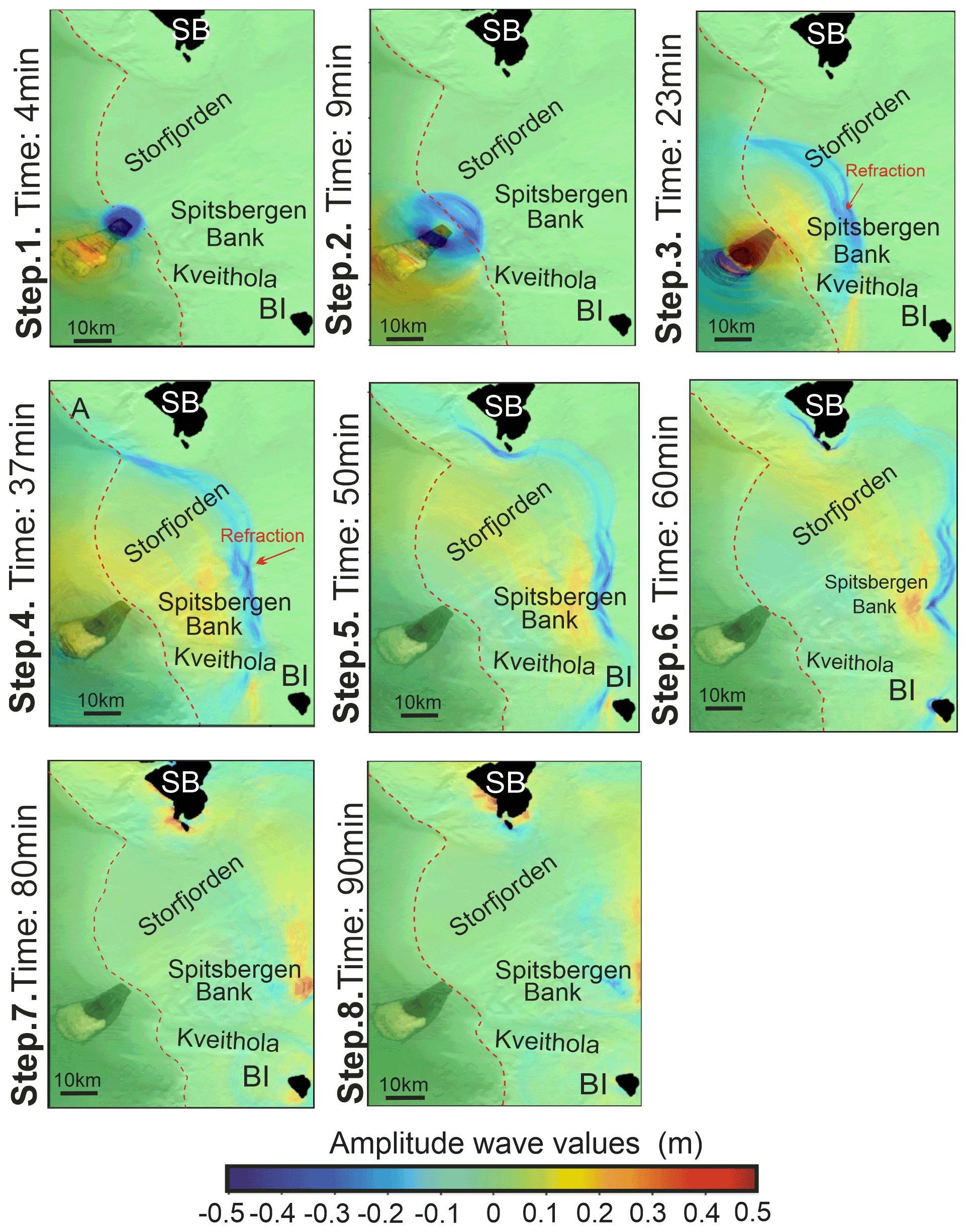
Figure 8 Eight steps displaying the tsunami waves generated at different times. The dotted red line indicates the shelf break. The first step shows the generation of the tsunami wave and its spread. At 23 min the outgoing wave suffers refraction. At 50 min the tsunami wave arrives at the northern coast of Spitsbergen and Bear Island, and at the 60 min, it hits the westernmost coast of Spitsbergen.

The tsunami arrival times are observed based on the propagation direction toward the coast. The impact of tsunami waves affects Sørkappøya at 50 min (southern Spitsbergen), with a trough amplitude value of 0.3 m, increasing to a crest amplitude value of 0.2 m at 75 min (Fig. 8, step 5; Fig. 9h). At the same time (50 min), the impact occurs at Kapp Dunér (northwestern Bear Island) with tsunami waves having a crest amplitude value of 0.3 m at 50 min, which increases to 0.5 m at 53 min (Fig. 8, step 5; Supplement video 2). After these two first coastal impacts, the tsunami affects different parts of both islands at different times. Southwestern Bear Island is reached by the tsunami waves at 60 min with a maximum crest amplitude value of 0.5 m (Fig. 8, step 6), followed by a trough amplitude value of 0.5 m at 65 min. Likewise, the north of Bear Island is affected by a trough amplitude value of 0.5 m (Fig. 8, step 6) and a crest amplitude value of 0.5 m at 80 min (Fig. 8, step 7). In Svalbard, Stormbukta Bay (southwestern Spitsbergen Island) is the next impacted coastline (Fig. 9a). There, the tsunami waves show specific velocity of v_s= 13 m s⁻¹ (at 18 m of depth), with trough amplitude values of 0.3 m at 63 min that increase crest amplitude values up to 0.32 m (85 to 95 min) (Fig. 8, steps 7 to 8; Fig. 9i). Finally, tsunami wave series propagating toward the coast occur until 2 h after the Storfjorden LS-1 landslide triggering (Supplement video 2).

Figure 9 Synthetic marigrams. (a) The location map of the synthetic marigrams above the reference stations, numbered in panel (a) (station 1 to 8). (b–i) Note the different arrival times, periods, wave heights and polarities at the different stations.

5 Discussion and conclusions

The L-ML-HySEA landslide tsunamigenic model provides a fast and consistent method for simulating landslide dynamics, tsunami wave generation, propagation and coastal impact. The results reveal several fundamental insights regarding the assessment of the main factors that control the characteristics and evolution of the Storfjorden LS-1 tsunamigenic landslide, as well as the related coastal hazard.

The submarine landslide geohazard studies are not easy to conduct due to the difficult access that the marine environment imposes, which makes it hard to obtain accurate analysis and monitoring. Our case study suggests that numerical modelling is of great help in understanding the dynamics of submarine landslide geohazard and their tsunamigenic potential. The Storfjorden upper continental slope presents critical conditions that need to be taken into account and warrants carrying out studies to assess slope stability. Several factors support this assertion: (i) the overpressure ratios measured in the subsurface sediments (Lucchi et al., 2013; Llopart et al., 2019) and (ii) the seismicity related to the active Hornsund Fault Zone (Hampel et al., 2009; Auriac et al., 2016; Pirli et al., 2013). In addition, (iii) the recent environmental stress represented by the factors mentioned above may intensify processes such as gas hydrate dissociation and fluid flow migration (León et al., 2021). Lastly, (iv) unloading rebound seismicity during ice retreat/melting (Berndt et al., 2009) also may contribute to triggering new submarine landslides.

5.1 Landslide dynamics and wave generation

Key landslide parameters for the generation of tsunamis commonly include volume, velocity and initial acceleration of the sliding mass (Harbitz et al., 2006; Urlaub et al., 2013; Løvholt et al., 2015; Macías et al., 2015; Urgeles et al., 2019) (Table 1). In our case study, the relationship between the above-mentioned parameters is also fundamental for the formation of a tsunami. The L-ML-HySEA model indicates that the 40 km³ of available displaced sediment volume moved by the Storfjorden LS-1 landslide is enough to trigger a tsunami. The morphosedimentary characteristics of the Storfjorden LS-1 landslide suggest that mass failure deposits could occur as a single event, as opposed to several, implying a better energy transfer to the water column (Vázquez et al., 2022, and references therein); therefore, velocity and initial acceleration also would be key to the formation of the tsunami. In this sense, for the phase velocity to be highly effective at the depths of Storfjorden LS-1 (H= 420 to 1900 m) during the tsunami wave onset, its value should be v_ta= 136 m s⁻¹ (Tinti et al., 2000; Fryer et al., 2004). The relatively average velocity (roughly 25 m s⁻¹, Table 1) obtained for our tsunami indicates that it was out of phase, and, therefore, it would not have been effective enough to create high-amplitude tsunami waves (Huggel et al., 2005; Evans et al., 2009; Pudasaini, 2014; Dietrich and Krautblatter, 2019).

Our results indicate that the characteristics of the tsunami wave are influenced by landslide dynamics at two stages of the downslope moving mass: initial (1 to 4 min) and late (20 to 25 min), with different velocity values (Fig. 6). The two initial wave dipoles, generated when seafloor failure occurs, are the consequence of two large seafloor depressions, one at the slide scar (i.e. main evacuation area) and the other one located between the two mass moving domains (Fig. 7 and Supplement video 1). At 25 min, a new dipole is formed, opposite to the previous ones. This new dipole is created when the faster sliding mass reaches the slower one and both masses merge producing a significant impact in the available displaced sediment thickness (100 m) of the distal moving mass. The increase in thickness would contribute to increasing the pressure in the water column, causing the uplift in the water surface and the enhancement of the tsunami waves (Ramadan et al., 2018; Ercilla et al., 2021). Thus, our study demonstrates that a proper understanding of landslide dynamics at their initial stages (or first motion) and of their deformation during the run-out is a crucial requirement for understanding the characteristics of the initial tsunami waves and the effects that those characteristics have on their evolution. In addition, our study also suggests that identifying the initial tsunami wave forms could reveal the tsunami sources, e.g. landslides (generating single or multiple trough and crest pairs) versus faults (generating a single or crest wave) (e.g. Macías et al., 2015; Ercilla et al., 2021; Estrada et al., 2021; Bécel et al., 2017).

5.2 Seafloor morphology

It is widely known that how a tsunami wave propagates is highly dependent on the morphology of the seafloor (Urlaub et al., 2013; Estrada et al., 2021). The model shows that tsunami waves propagate elliptically with respect to the northeast–southwest elongated seafloor shape of the landslide relief. In the Storfjorden LS-1 tsunami, the average velocity waves (v_ta= 136 m s⁻¹) travel northeastern and are focused between the continental shelf of Svalbard and of Bear Island, which helps to confine it and forces its direction of propagation (Fig. 8 and Supplement video 2). The continental shelf morphology determines tsunami shoaling, with the shallowest water depths located at Spitsbergen Bank (80 m water depth). The shoaling by the bank produces the refraction phenomenon and the amplification of the tsunami. As the tsunami propagates across the ocean, waves can undergo refraction, which is caused by segments of the wave moving at different speeds as the water depth along the wave front varies (Berkhoff, 1972). This effect produces variations in the amplitude of the tsunami waves and in their arrival times: 15 min later at southwestern Spitsbergen and 11 min later at northwestern Bear Island. When encountering an obstacle, the tsunami waves discharge their energy with great force, as in the case of Sørkappøya and Sørkapp at 75 min, decreasing the amplitude and slowing down the arrival time of the tsunami waves in the corresponding bay to 100 min (Supplement video 2). The tsunami wave arrival is recorded at 80 to 95 min at the eastern Hornsund fjord. On the other hand, the crescent shapes of the tsunami front seem to be conditioned by the Storfjorden and Kveithola glacial troughs separated by Spitsbergen Bank. The elongated negative reliefs of the glacial troughs would cause the funnelling of the tsunami seawater with relative higher specific velocities of propagation (v_s= 56 m s⁻¹ in the Storfjorden glacial trough at 320 m water depth). Therefore, the numerical simulations are a useful tool to assess tsunami hazard in places where local seafloor topography could advance or delay the tsunami waves and therefore the coastal impact.

The Storfjorden LS-1 modelling has demonstrated that the shelf seafloor morphology is a decisive factor: it influences the propagation velocity of the tsunami waves, the variations in wave amplitude (shoaling effect) and the impact of coastal arrivals (Iglesias et al., 2012; Estrada et al., 2021; Salaree and Okal, 2020).

5.3 Coastal location

The initial tsunami waves start propagating as negative and positive disturbance dipoles. The trough is always located towards the upper part of the margin, which determines that, in general, the first arrival to the coast corresponds to a sea level drop, hence decreasing the coastal impact. This factor, together with coastal location and orientation (i.e. angle of the waves with the coastline), conditions the polarities of the first arrival wave. In our study, the first arrival wave impacted with trough values of 0.1 to 0.5 m against the coast of southwestern Spitsbergen and crest values of 0.1 to 0.5 m against Bear Island (Fig. 8 and Supplement video 2).

5.4 Comparison with other landslide tsunamis: hazard assessment for the northern glaciated margins

Landslide parameters (age, area, volume, seafloor gradients, location and velocity) and related tsunami parameters (wave amplitude and velocity) of different landslide-inducing tsunamis have been compared with those defining Storfjorden LS-1 and its tsunami, in Table 2.

Table 2 Submarine landslides compared with Storfjorden LS-1. In the trigger column, the letters represent (A) weak-layer sedimentary architecture, (b) earthquake, (c) gas hydrate dissociation and (d) other additional factors. Deposit type: mass wasting (MW), large rafted blocks (LRBs), turbidity currents (TCs), debris flows (DFs) and slump blocks (SBs). References: Storfjorden LS-1 (Pedrosa et a., 2011; Lucchi et al., 2012; Rebesco et al., 2014; Llopart et al., 2015), Hinlopen (Winkelmann et al., 2008; Vanneste et al., 2006), Bjørnøyrenna (Laberg et al., 1999), Gebra Valley (García et al., 2009; Casas et al., 2013), Grand Banks (Piper et al., 1999; Fine et al., 2005), Storegga (Haflidason et al., 2004; Bondevik et al., 2012), Kongsfjorden TMF (Berndt et al., 2009), Trænadjupet (Laberg et al., 2002), Nyk (Lindberg et al., 2004), Skagway (Thomson et al., 2001; Synolakis et al., 2002), Lituya Bay (González-Vida et al., 2019) and BIG'95 (Iglesias et al., 2012).

This comparison highlights that not only large but also relatively small–medium-sized landslides could have triggered tsunamis in the past. Despite Storfjorden LS-1 having a smaller area and volume with respect to the larger landslides of the Kongsfjorden TMF, the amplitude value of their respective tsunami waves is roughly similar. The effects of global warming over the landslide-triggering factors (e.g. isostatic rebound seismicity and gas hydrate destabilization by the rise in temperature of the ocean water) is not likely to provoke the occurrence of such large landslides as those formed during glacial maxima and the transition from glacial to interglacial periods (Lee, 2009, and references therein). However, the present trend of global warning should over time increase the probability of slope instability, especially on those glaciated margins that have not yet failed after the last glacial to interglacial transition, for instance, the Bear Island, Kongsfjorden and Storfjorden TMFs (Berndt et al., 2009). Therefore, the results presented here should encourage us to continue working in the prediction of tsunamigenic landslide hazards and their coastal impact, mainly in the northern glaciated margins.

The water depth location of the landslide scar seems to influence the coastal impact of tsunami waves (Table 2). In the study area, they present low-amplitude values at the coastal area and their arrival times are longer (50 to 80 min) than the tsunamis modelled in the nearby coast of western Spitsbergen (Bernt et al., 2009), where the slope failure is at shallower water depths (200 m) and the distance to the nearby coast is shorter (∼ 90 km). Landslides triggered in shallower water result in more localized waves, and the elongated landslide velocity profile delays the appearance of the first positive landward-propagating wave, hence reducing the chances of constructive interference along the coast (Harbitz et al., 2006). This suggests that tsunami modelling based on past landslides should pay more attention to those sectors of the northern glaciated margins with narrower continental shelves and submarine landslide head scarps that are near the shoreline. The landslides located in the middle and northern parts of Norway are a good example of that (L'Heureux et al., 2013; Beaten et al., 2013). Also, much smaller collapses, either submarine or subaerial, also pose a significant local threat. In Norway, several rockslide tsunamis occurred in the 20th century, the most devastating in Storfjorden in 1934 (Blikra et al., 2005; Böhme et al., 2015). Although this is not the scope of the paper, they could be more frequent with an estimated rate of 1 event per 1000 years (Blikra et al., 2005).

In summary, our findings demonstrate that tsunami modelling based on past landslides using the L-ML-HySEA landslide tsunami model will be useful to provide new perspectives on tsunami hazard assessment in polar margins, where global climatic change and its related ocean warming may contribute to the activation of landslides. Landslide tsunami models will allow us to identify the areas with maximum and faster coastal impact and the effect of the local bathymetry on tsunami direction of propagation, shoaling, amplification and diffraction. This knowledge is very important for the design of early-warning strategies, as it will contribute to assess the key factors that are useful as emergency planning tools.