the Creative Commons Attribution 4.0 License.
the Creative Commons Attribution 4.0 License.
 | 21 Nov 2022
Analysis of the relationship between yield in cereals and remotely sensed fAPAR in the framework of monitoring drought impacts in Europe
Carmelo Cammalleri
Niall McCormick
Andrea Toreti
This study focuses on the relationship between satellite-measured fraction of absorbed photosynthetically active radiation (fAPAR) and crop yield cereals in Europe. Different features of the relationship between annual yield and multiple time series of fAPAR, collected during different periods of the year, were investigated. The two key outcomes of the analysis are the identification of the period: (i) from March to October as the one having the highest positive correlation between fAPAR and yield and (ii) from February to May as the period characterised by most of the estimated negative correlation. While both periods align well with the commonly assumed dynamic of the growing season, spatial differences are also observed across Europe. On the one hand, the Mediterranean regions report the highest correlation values (r>0.8) and the longest continuous periods with positive statistically significant results (up to 7 months), covering most of the growing season. On the other hand, the central European region is characterised by the most limited positive correlation values, with only 2 months or less showing statistically significant results. While marked differences in the overall capability to capture the full dynamic of yield are observed across Europe, fAPAR anomalies seem capable of discriminating low-yield years from the rest in most of the cases.
- Article
(8743 KB) - Full-text XML
- BibTeX
- EndNote


Drought is a multifaceted phenomenon threatening societies, economies, and ecosystems in a complex web of cascading effects (UNDRR, 2021). Among the major sectors that are impacted by drought, agriculture is still recognised as the most sensitive one (FAO, 2015, 2021; FAO et al., 2018), as reflected by the large share of reported impacts for agriculture over the majority of countries and drought events in Europe (Stahl et al., 2016).
Most drought monitoring systems recognise the prominent role of agricultural drought by refining indicators of meteorological drought in order to better account for impacts on vegetation growth (e.g. the standardized precipitation–evapotranspiration index – or SPEI; Vicente-Serrano et al., 2012) and/or by directly incorporating drought indicators that are based on remotely sensed vegetation indices (WMO and GWP, 2016). In particular, negative deviations from climatological values of satellite measurements of vegetation “greenness” – for example, the standardised anomalies of the fraction of absorbed photosynthetically active radiation (fAPAR) that are provided by the European Drought Observatory and the Global Drought Observatory (EDO and GDO, https://edo.jrc.ec.europa.eu, last access: November 2022) – are often adopted as a proxy variable for the adverse effects of drought on vegetation.
While such approaches are logically based on the connection between reduced vegetation greenness and diminished plant productivity, it is also well known that droughts occurring during different phenological stages may have different impacts on yield and production (i.e. Barros et al., 2021; Ceglar et al., 2020; Chaves et al., 2002; Demirevska et al., 2009; Monteleone et al., 2022; Stallmann et al., 2020; Zampieri et al., 2017). Consequently, greenness anomalies are not always directly related to reduction in yield, depending on the development stages of the vegetative cycle when they manifest. Some studies have tried to account for this concept by limiting the analysis to the growing period and excluding data for the plant dormancy phase (e.g. Rojas et al., 2011), by deriving key variation metrics (i.e. amplitude, integral, maximum) from the full growing season (e.g. Kang et al., 2018), or by focusing only on key periods (i.e. a specific month) that have been shown to correlate well with deviations in annual yield for a given study area (Bachmair et al., 2018).
Within the framework of the near-real-time monitoring of drought events, the task of evaluating and quantifying the actual relevance of an observed anomaly in vegetation greenness is complicated by the need to continuously update the status based on newly acquired data, without the benefit of the full picture of the complete vegetation cycle. This limits the possibility to implement some of the above-mentioned approaches as part of operational drought monitoring systems, beyond the simple masking of data acquired outside of a predefined period (e.g. the growing season). An example of an early warning system that accounts for the timing of the observed anomalies is the Anomaly Hot Spots of Agricultural Production (ASAP) decision support system (Rembold et al., 2019), where the seasonal progression (expansion, maturity, senescence) is explicitly considered in determining the warning level.
As part of the shift in the drought risk management paradigm from a reactive to a proactive approach, the move from simple hazard indicators to quantitative assessments of risk and impacts is likely to be further integrated within modern early warning systems (UNDRR, 2021). In this regard, independent estimates of actual drought impacts, such as the information that can be derived from records of yield deviations for different crop types, constitute a valuable reference. Unfortunately, this information is often collected at coarse spatial resolution and is available with a significant temporal delay. It is however very valuable to assess if anomalies in vegetation indices can be used to detect the effects of drought conditions and how their robustness as proxy for yield reduction varies in space and throughout the year. This can also enable the successive evaluation of the efficiency of remotely sensed indicators as a proxy for the effect of drought on vegetated land, and the refinement of their use as stress-forcing data for agro-economic models for the assessment of losses in agriculture due to droughts (García-León et al., 2021).
In this context, the primary goal of this study is to analyse to what extent the year-by-year dynamics of yield in Europe can be explained by a regularly updated operational vegetation drought indicator, in particular by the fAPAR anomalies produced by EDO. Yield data for cereals, recorded by Eurostat, are here used as a starting quantity to produce records of anomalies in yield at European scale. The spatio-temporal variations in the relationship between dekadal (i.e. 10 d) fAPAR anomalies and yearly yield deviations can help in identifying the periods of the year when fAPAR represents a reliable proxy information of yield reduction impacts in Europe. This would prove a quantitative basis for improving the assessment of drought impacts in agriculture, with potential benefits both for drought monitoring systems and for agro-economic models.
2.1 Eurostat yield dataset
Eurostat, the European Statistical Office, publishes regular reports of statistics on annual crops, including data on production, cultivated area, and yield for different crop types, at both national and sub-national aggregation levels (Eurostat, 2020), with the aim of providing a harmonised database of data collected by EU Member States and neighbouring countries.
For the purposes of this study, annual yield data on cereals (wheat and spelt, rye, barley, oats, grain maize, triticale, and sorghum) have been retrieved between 2001 (first full year with available fAPAR data) and 2018 (last available year in the Eurostat database at the time of this study), mostly at the spatial scale of Eurostat's so-called “NUTS 2” regions (hereafter referred to simply as regions). Only in the case of Germany and the UK were data at the NUTS 1 level used in order to maximise both data coverage and consistency in region size with the rest of the domain.
Since yield data are to be used for computation of deviations from the long-term average, temporal consistency in the data records is essential. For this reason, records that are flagged by Eurostat as estimated, provisional, unreliable, or with a definition that differs due to missing components were excluded from the analysis.
Systematic changes in the annual yield time series were removed by applying a Savitzky–Golay filter to account for advancement in technology and crop management (Tadesse et al., 2015), before standardised anomalies were computed only for those regions with more than 9 years of data (i.e. half of the analysed period). A linear de-trending was also tested (not shown), but a limited effect of this choice was observed on the obtained yield anomalies time series. Following this procedure, 240 regions with valid time series were obtained (out of the 267 regions considered at the start of the study).
2.2 MODIS fAPAR dataset
The fraction of absorbed photosynthetically active radiation (fAPAR) is one of the 50 essential climate variables recognised by the UN Global Climate Observing System (GCOS), mainly thanks to its direct relationship with primary production (https://gcos.wmo.int/en/essential-climate-variables/fapar, last access: November 2022).
fAPAR, and in particular its deviations from historical climatology, constitutes the ideal proxy variable for the effects of drought on vegetated lands (Rossi et al., 2008). In this context, remote sensing images collected by the MODerate resolution Imaging Spectroradiometer (MODIS) sensor represent a unique data source for drought studies due to the unprecedented longevity of the Terra satellite.
In this study, the standard MODIS Terra LAI/fAPAR product (i.e. MOD15A2H, Collection 6) is used (Myneni, 2015), in which global fAPAR maps are derived from the atmospherically corrected bidirectional reflectance distribution function (BRDF) recorded by MODIS in seven spectral bands, by solving the three-dimensional radiation transfer process through a look-up-table approach (Knyazikhin et al., 1998; Wang et al., 2001).
The standard MODIS product is distributed as 8 d composites (using a maximum composite method) at a spatial resolution of 500 m in 1200 km×1200 km tiles on a sinusoidal grid. Data include a quality assessment (QA) layer that allow for the detection of where the simplified back-up algorithm has been used.
Datasets of both fAPAR and fAPAR anomalies based on MOD15A2H raw data are regularly produced as part of the European Drought Observatory and the Global Drought Observatory (EDO and GDO, https://edo.jrc.ec.europa.eu, last access: November 2022) of the EU's Copernicus Emergency Management Service. The operational fAPAR dataset is obtained after a set of pre-processing procedures, including (1) screening of the low-quality data based on the QA flag layer, (2) spatial aggregation of the data (simple average) at 1 km resolution and re-projection onto a lat–long regular grid at 0.01∘ resolution with nearest neighbour resampling, (3) temporal aggregation at dekadal scale (three maps per month: days 1–10, 11–20, and 21–end-of-month) by means of a weighted average of the two closest 8 d images (weight proportional to the overlapping with the dekadal period), and (4) exponential temporal smoothing of the dekadal data (with smoothing parameter equal to 0.5; Brown and Meyer, 1961).
Here, the fAPAR anomalies were computed as standardised deviations from the reference period (2001–2018), only if at least 6 years of data were available and only where the long-term standard deviation was greater than 0.01 (to exclude areas of low variability, such as deserts or highly stable densely vegetated areas). The reference period of 2001–2018 is consistent with the one used for yield anomalies.
2.3 Analysis strategy
In this study, the analysis of the relationship between the dekadal time series of fAPAR anomalies and yearly crop yield is based primarily on the Spearman correlation coefficient (r). In order to carry out the analysis, the two main discrepancies between the two datasets, namely regarding the spatial units (i.e. regions versus cells) and temporal frequency (year versus dekad), must first be considered.
Given the focus of the study, the only fAPAR conditions that are relevant are the ones observed over arable land. Therefore, the fAPAR anomaly data were first upscaled to NUTS 2 regions as a weighted average of all the 0.01∘ resolution fAPAR anomaly values within a region, with a weighting factor based on the fraction of each grid cell classified as arable land according to the latest Corine land cover map (CLC2018, https://land.copernicus.eu/pan-european/corine-land-cover/clc2018, last access: November 2022). This masking allows for removing from the NUTS 2 average all grid cells where the fAPAR dynamics are not related to agriculture (e.g. forest and urban rural areas).
Regarding the temporal frequency, while fAPAR anomaly data are available throughout the year, similar studies (e.g. Rojas et al., 2011) have focused only on data collected during the growing season. A north-to-south gradient has been observed at the start, at the end, and for the length of the growing season in Europe, with April–September being a common period all over Europe, but with an early start in February and a late end in November over many areas (Rötzer and Chmielewski, 2001). Estimations of the growing season directly based on remotely sensed vegetation indices have also highlighted a very early start in the Mediterranean, around October/November of the previous year (i.e. Atzberger et al., 2014), likely related to combined effects (e.g. infesting weeds, early sowing, and emergence) on the remote sensing signal. Following these considerations, here we analyse an extended period, testing the relationship between the yield of a particular year and the fAPAR anomalies between the first dekad of October of the preceding year and the end of the current year, for a total of 45 dekadal time series.
The set of correlation analyses between each of the 45 dekadal time series of fAPAR anomalies and yearly yield data is used to construct a “correlogram”, which relates the dekad with the corresponding r value. The example of the Tuscany region in Italy (Fig. 1) highlights some common behaviours of the correlogram, such as a relative smooth transition between periods of positive and negative r values. Different analyses can be performed, depending on the critical values that are extracted from these plots and on the goal of the analysis. Here, we faced a problem in two different ways: (a) detecting periods of similar behaviour and accuracy but variable length and (b) detecting periods of similar length but variable accuracy and behaviour.
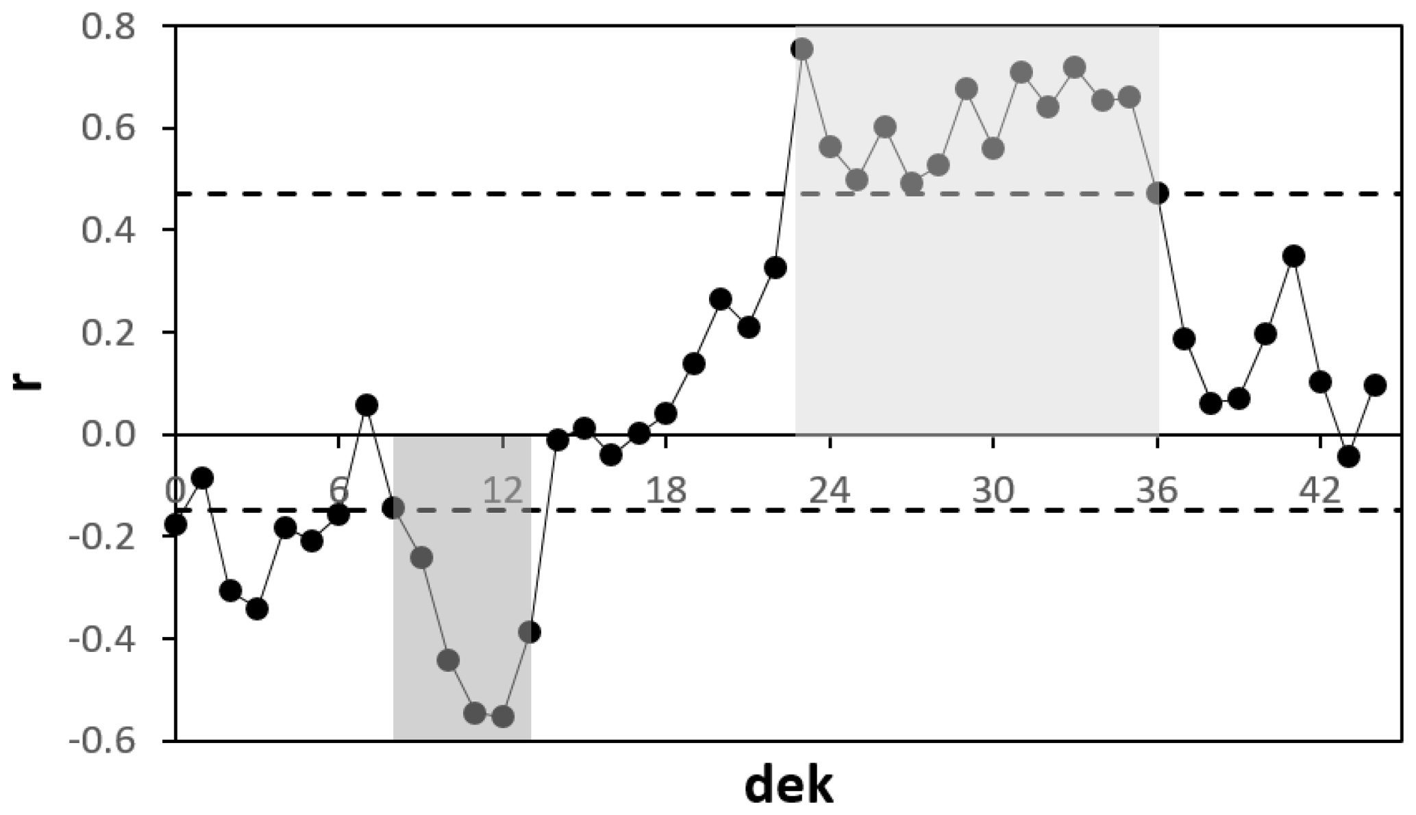
Figure 1Example of correlogram for one NUTS 2 region in Italy (ITI1, Tuscany). Each value represents the Spearman correlation coefficient between the fAPAR anomaly time series of a specific dekad and the yearly yield anomalies. The two horizontal dashed lines respectively represent the threshold for a positive statistically significant value at p=0.05 and the minimum negative threshold (, see the main text). Dekads are defined starting from the first one of October of the previous year (e.g. dek=23 refers to the last dekad of May of the current year).
For these two analyses, we distinguished between two different behaviours in the fAPAR–yield relationship, a direct relationship (i.e. negative anomalies in fAPAR correspond to negative anomalies in yield) and an inverse relationship. The latter may occur when strong vegetative growth is observed early in the season during drought years, especially in energy-limited conditions (van Hateren et al., 2021). We also distinguished between two levels of accuracy, statistically significant correlations (p<0.05, either positive or negative) and a less stringent condition where at least different than zero r values (i.e. ) are considered. This second tier of values represents those conditions where a statistically significant correlation (at p<0.05) is not achieved, but a positive/negative relationship can still be estimated. A value of 0.15 is used, as it corresponds to roughly of r at p=0.05 in the case of a full sample.
By defining a period as a streak of consecutive dekads of length (L) between 2 and 45, 990 periods of various length can be analysed for each region, and for each of these periods four main metrics (ranging between 0 and 1) are computed: (1) Fp+, the fraction of r values in the period that are positive and statistically significant (i.e. r>0 and p<0.05); (2) Fp−, the fraction of r values in the period that are negative and statistically significant (i.e. r<0 and p<0.05); (3) F+, the fraction of r values in the period that are at least positive (i.e. r>0.15); and (4) F−, the fraction of r values in the period that are at least negative (i.e. ). By definition, F+ and F− are always greater than or equal to Fp+ and Fp−, respectively. We can then focus on the longest periods (among the 990 periods) having homogeneous behaviour and accuracy for a given region (homogeneous periods hereafter), e.g. a period with . Due to the smooth dynamics observed in most correlograms, these homogeneous periods are rather well defined. In the rare instances when multiple homogeneous periods of the same length are found for a region, the period closer to the surrounding regions is selected.
In the example reported in Fig. 1, the dekads between 23 and 36 (light grey area) are clearly part of the longest period with all positive and statistically significant r values, L=14, while the dark grey area demarks the longest period with (L=6).
A further set of analyses is focused instead on a fixed time window selected among a limited range of lengths of the periods (i.e. a subset of periods among the 990 possible periods with length from 2 to 45). The boundary values of this subset of periods can be derived from the previous tests. Within these limits, an optimal positive (negative) period for each region can be defined as the period with the maximum (minimum) average r value. Differently from the first group of analyses, these optimal periods have varying Fp+ and F+ values (corresponding to the average r value) that can be used to quantify the robustness of the relationship between fAPAR and yield. This analysis is performed on a subset of periods to avoid selecting as optimal very short periods (i.e. of length 2) for regions with a prominent peak value or very long periods for regions where the correlogram is particularly flat.
Finally, while the analyses based on correlation give insight to the relationship between fAPAR and yield over the full spectrum of variability, a further test focused only on extreme low yields is also performed, given that in the context of drought monitoring it would be sufficient to be able to distinguish these conditions from the rest in order to successively detect the drought-affected years. Here, the total number of cells for each region with fAPAR anomalies (a common threshold used in extreme analyses) is computed during low yield years (yield anomalies ), and it is compared with the same during the other years (yield anomalies ). The assumption of this analysis is that the ratio of these two quantities should be greater than 1 in the case of a direct relationship.
3.1 Dynamics of yield anomalies and relationship with droughts
While negative anomalies in yield can often be associated with drought events, the full dynamic of standardised yield anomalies for cereals, as described in Sect. 2.1, cannot be exclusively ascribed to the occurrence of drought conditions. However, the ability to capture the year-by-year dynamics of yield using fAPAR anomalies is evaluated here with the goal of exploiting this relationship in the framework of drought monitoring, and hence the connection between low yields and droughts needs to first be assessed.
Figure 2 depicts the temporal evolution of yearly yield deviations, highlighting some clear spatial patterns of significantly negative anomalies (i.e. yield anomaly ). Following a review of the scientific literature for past drought events, it is possible to associate a documented main drought event with many of these large clusters, as summarised in Table 1. Seven main droughts are reported, ranging from the well-known drought in central Europe in 2003 (Rebetez et al., 2006) to the central–northern European drought of 2018 (Buras et al., 2020; Toreti et al., 2018).
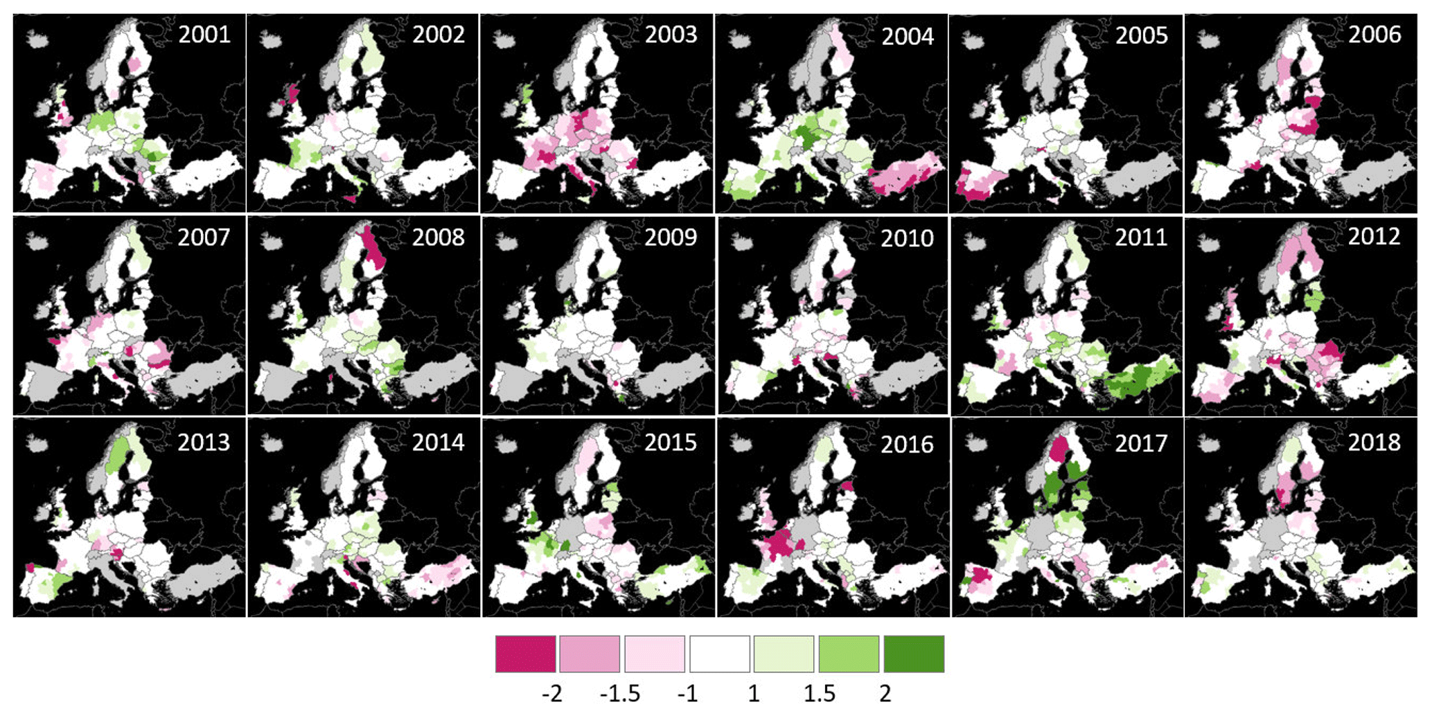
Figure 2Spatial distribution of annual standardised yield anomalies for the period 2001–2018. Anomalies are mapped at NUTS 2 level, with the exception of the areas detailed in Sect. 2.1. Data in grey are missing.
The existence of a cause–effect relationship between these largest spatial patterns observed in negative yield anomalies and the listed major drought events is further supported by the study of Spinoni et al. (2015), which categorised the listed events (except the last two, which occurred after that study) as being among the most severe in Europe according to meteorological drought indices.
Table 1Main European drought events between 2001 and 2018 corresponding to the large patterns in negative yield anomalies () observed in the maps reported in Fig. 2. References to the scientific literature of each event are also reported, with a brief description of the documented impacts for the agriculture sector.

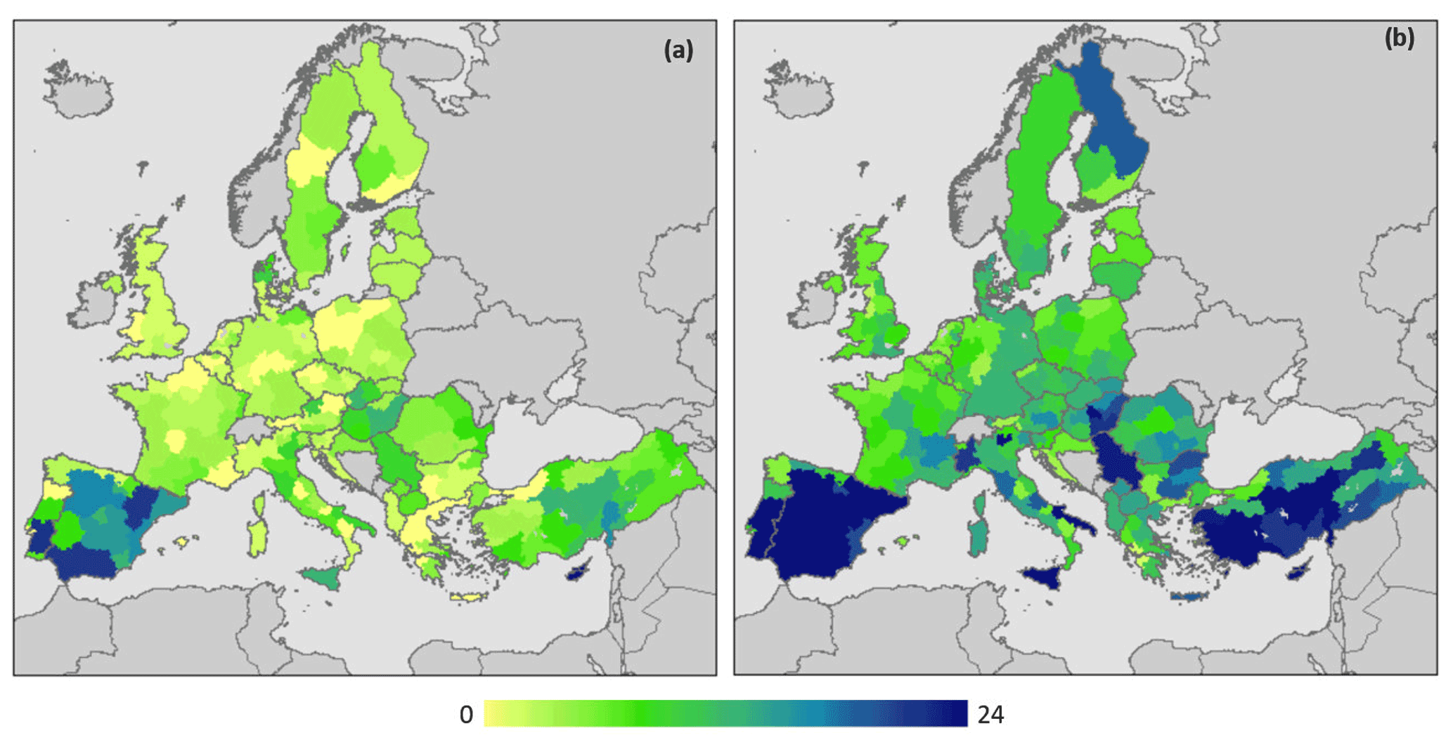
Figure 3Spatial distribution of the length (in dekads) of the longest period with (panel a) and (panel b).
For each of the drought events listed in Table 1, specific independent scientific references are also provided, which include details on the evolution of the meteorological conditions and the potential impacts on agriculture. Overall, analyses of these data tend to support the fact that the adopted dataset of yield anomalies shows the impacts on vegetation of the major European droughts, in conformance with the conclusions of other studies at regional level in Europe (Bachmair et al., 2018; Potopová et al., 2015), or for other parts of the world (e.g. Yang et al., 2020).
3.2 Detection of the homogeneous periods in the fAPAR–yield relationship
While many studies focused on the local maximum r value to detect when and where fAPAR and annual yield anomalies best correlate, isolated peak values may alter the perception of the robustness of fAPAR as a proxy variable for yield. In the context of an operational drought monitoring system, where continuous estimates should be provided rather than “one shot” predictions, information on longer homogeneous time periods is more valuable.
Focusing first on the positive r values, we analysed the periods with only statistically significant values (), or only at least positive values (). The maps in Fig. 3 report the local maximum lengths corresponding to these two quantities, namely positive homogeneous periods. Both of these maps show generally longer homogeneous periods in southern Europe, with the largest values observed for some Mediterranean regions (e.g. most of Spain, Cyprus, Sicily, Apulia, and Aegean–Mediterranean Turkey), and the smallest values (or no homogeneous period at all) mostly located in central Europe (i.e. Germany, Poland, and north-eastern France). On average, the maximum length of the periods with is limited in most of the cases (5.5 ± 4.3 dek, almost 2 months), whereas the values more than double in the case of (13.0 ± 8.3 dek, more than 4 months).
Generally, almost all the maximum r values in the correlograms are obtained in the dekads between mid-February and mid-September, which is expected since this period aligns well with what is commonly considered the growing season in Europe (Atzberger et al., 2014; Rötzer and Chmielewski, 2001). Nonetheless, a large variability in the length of both positive homogeneous periods is observed, with southern and central Europe confirmed to be not only the areas with the highest and lowest r values, respectively, but also the areas with the longest (i.e. 4–7 months) and shortest (up to 2 months) periods with consecutive statistically significant positive correlations.
Due to the large variability in the length of the homogeneous periods observed in Fig. 3, a direct analysis of the spatial patterns in the starting and ending dekads is not feasible. So, in order to synthetically evaluate the temporal location of these homogeneous periods, we analysed which dekads each of them covers and computed for every dekad the fraction of NUTS 2 regions (out of 240) that includes that particular dekad in the homogeneous period (Fig. 4). For example, dekad 27 (i.e. the first dekad of July starting from the beginning of October of the previous year) is part of the maximum homogeneous period in about 20 % and 50 % of the regions, for Fp+ and F+, respectively. It is worth noting that about 21 % of the NUTS 2 regions do not have a period (minimum 2 consecutive dekads) with .
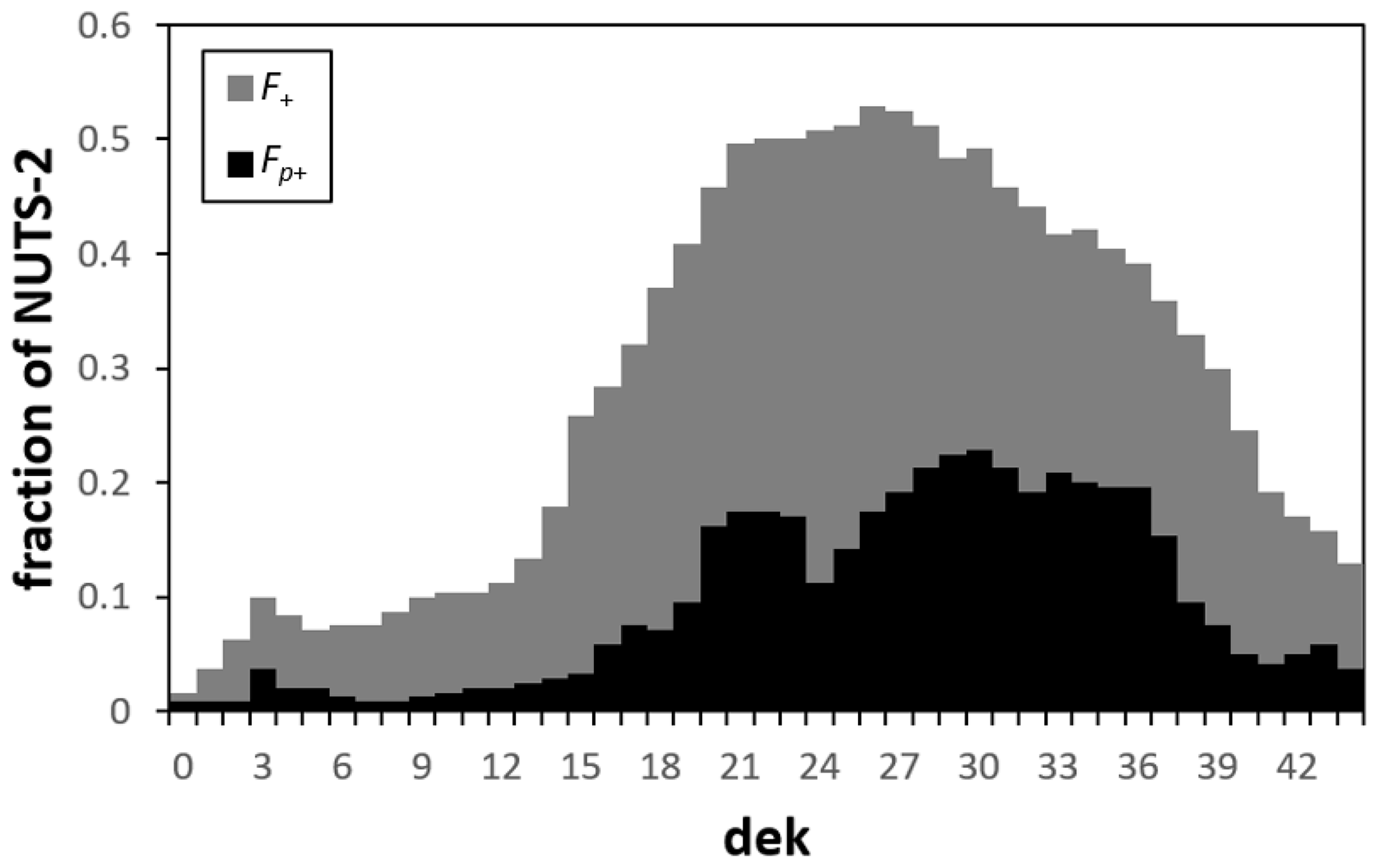
Figure 4Fraction of NUTS 2 regions for which each dekad is included in the longest homogeneous period with (black) or (grey).
It is possible to observe two “flexing points” in each of the two time series in Fig. 4 around 0.1 for Fp+ and 0.2 for F+. Starting from these values, we can detect two optimal homogeneous periods: from the end of April to mid-October (6 months) for Fp+ and from March to early November (8 months) for F+.
Moving to the negative correlation values, two maps analogous to the ones in Fig. 3 are reported in Fig. 5 for Fp− (panel a) and F− (panel b). These two maps show how the longest negative homogeneous periods are in general shorter than the ones for positive correlations, with an average value of 3.0 ± 1.6 dekads for Fp− and 7.0 ± 3.9 for F−. The lack of statistically significant negative r values is especially evident, with almost 50 % of the regions having no homogeneous periods with . The map for F− (Fig. 5b) allows for some additional considerations on the spatial distribution, with moderate maximum lengths (around 9 dekads) in most of western and central Europe and some high values (higher than 15 dekads) in some regions of southern Europe.
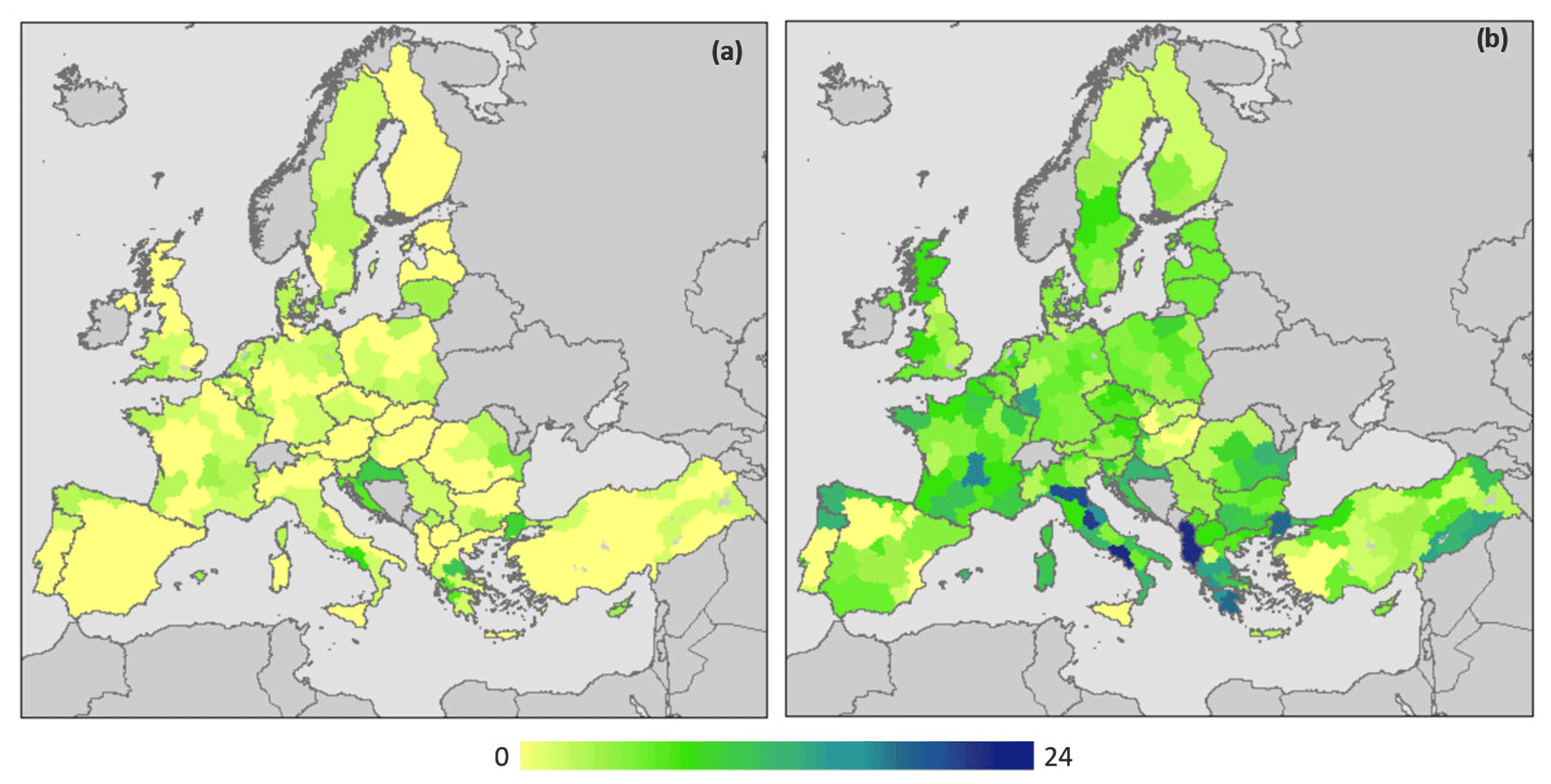
Figure 5Spatial distribution of the length (in dekads) of the longest period with (panel a) and (panel b).
In terms of temporal distribution, the histograms in Fig. 6 depict the fraction of NUTS 2 regions that includes that particular dekad in the negative homogeneous periods. Overall, the fraction values are lower than the ones observed for the positive periods (see Fig. 4), with two distinguishable peak periods in the F− values, the first in the early season (February–May) and the second after the end of the season (October–December, sowing period for the winter crops).
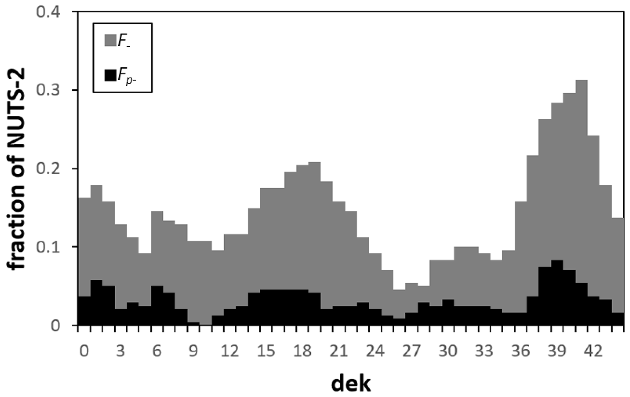
Figure 6Fraction of NUTS 2 regions for which each dekad is included in the longest homogeneous period with (black) or (grey).
Most of the homogeneous periods early in the season correspond to regions in western and southern Europe, and the late season periods are mostly located in central and northern Europe. In the framework of drought monitoring, the first can be potentially exploited as early warning signals of subsequent reduction in fAPAR due to drought (as seen in the positive homogenous periods that usually follow in the correlograms). The second mostly occurs right after the harvesting season and hence as no value for early warning systems.
3.3 Performance for a fixed time window
A clear outcome of the previous analyses is that the length of the homogeneous periods with negative correlations is limited compared to the positive correlations and mostly useful for drought monitoring only early in the growing season. Therefore, we focus only on the positive correlation values for the successive analyses. The two lengths (6 and 8 months) derived from the data depicted in Fig. 4 are used as the minimum and maximum boundary values to find the local optimal period for each region (see Sect. 2.3).
The results of this bounded analysis of the local optimal period are shown in Fig. 7, where the starting dekad (di, panel a) and ending dekad (de, panel b) of the optimal period are depicted for every region. Figure 7a shows a general pattern of an early start in central Europe (i.e. February/March) and in a few southern regions of the Mediterranean, as well as a late start (i.e. May/June) in most of southern and western Europe. This late start is of course in line with the previously observed negative correlations in February/May over the same regions. Analogously, Fig. 7b shows that the end of the optimal period occurs mostly around October/November, after the harvesting, in both southern and western Europe, and August/September in central Europe, with then mostly negative correlations in central and northern Europe occurring after this period (likely due to spurious correlations).

Figure 7Spatial distribution of (a) the starting dekad and (b) the ending dekad of the local optimal period based on the average correlation and bounded by a length from 6 to 8 months.
Given that these optimal periods have been derived based on the average r values in the 6- to 8-month period, the Fp+ and F+ values corresponding to these optimal periods can assume any values between 0 and 1 (no significant/positive r values to all significant/positive r values within the optimal periods). For this reason, we classified each region based on the combined values of these two metrics, as represented by the legend included in Fig. 8. In this map, the green areas show a good capability to reproduce the dynamic of yield deviation for the whole optimal period (the fraction of high r values in the two optimal periods is high), with the regions in dark green having the overall best performance (over half of dekads with statistically significant r values and more than with at least positive values). Conversely, the red regions show a poor capability of the fAPAR anomalies to capture the yield dynamics, with the dark red regions having less than of statistically significant values (i.e. less than a month) and less than of positive correlations during the optimal period.
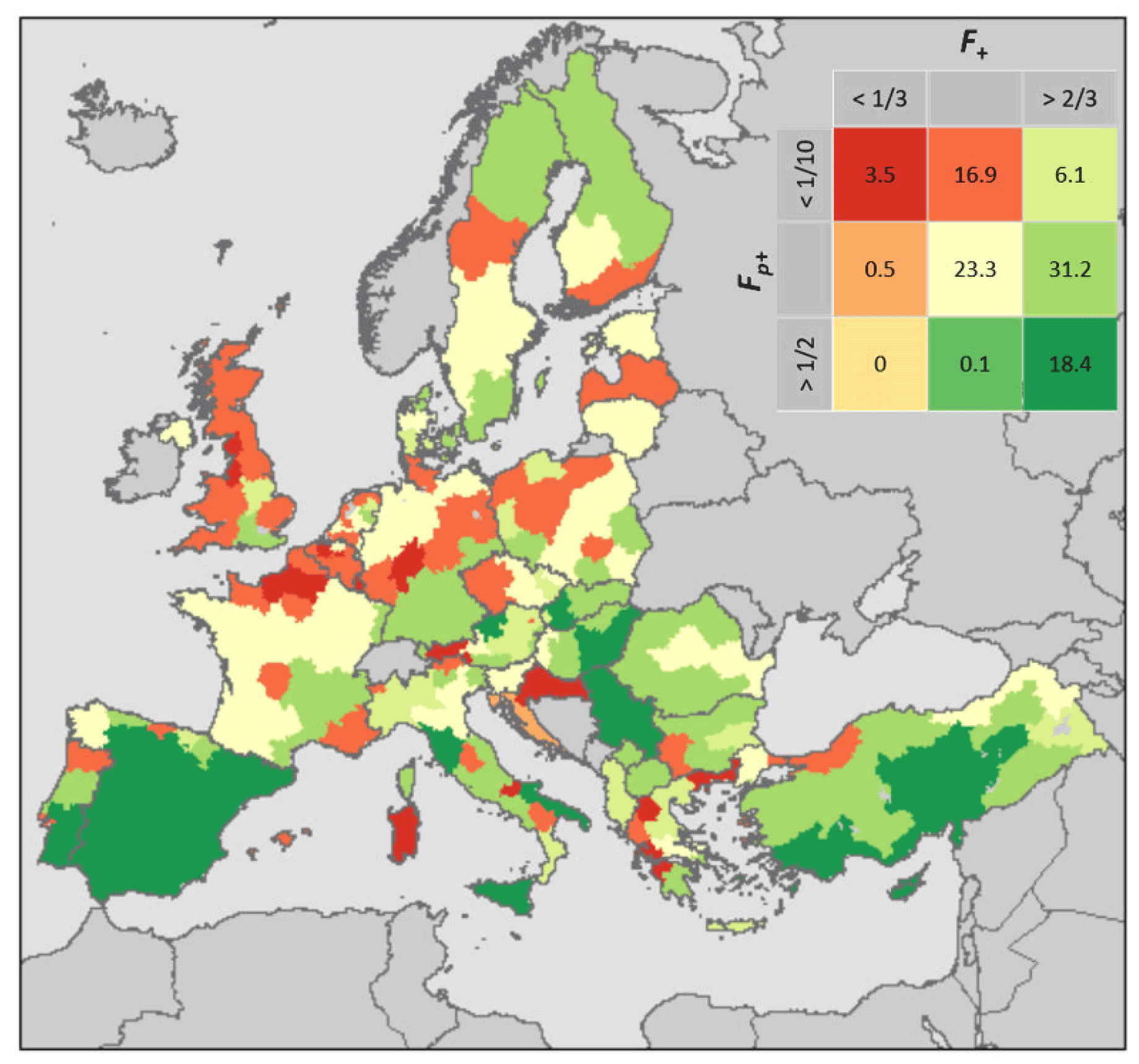
Figure 8Synthetic representation of the performance of dekadal fAPAR anomalies in reproducing the yearly yield variations during the local optimal period. The inserted legend shows the values of Fp+ and F+ for each category, with the numbers inside each square representing the percentage (%) of the total NUTS 2 regions (out of 240) that fall under each category.
Overall, slightly more than half (i.e. 55.8 %) of the study regions are classified in one of the green classes, with a predominance of these regions in the Mediterranean and south-eastern Europe. The rest of the study area is almost equally split between regions with average performance (yellow classes, 23.3 %), and poor performance (red classes, 20.9 %). Among the red classes, the majority of the regions fall in the category with intermediate F+ values () but low statistical significance (). Most of these regions are located in central Europe, between northern France, the United Kingdom, Germany, and Poland.
Spain stands out as having particularly robust performances, even among the generally good-performing Mediterranean area. While the start and end of the optimal period vary across the area (March to May, and September to November, respectively), the results are consistently in the best class (dark green in Fig. 8). Among the Mediterranean countries, some mixed results can be observed in Italy and Greece.
3.4 Detection of low yield years
The previous analyses show a noticeable difference in the performance of fAPAR anomalies to capture the full range of variability of yield anomalies across Europe, as quantified by the results on the optimal periods summarised in Fig. 8. For the same optimal periods, the number of fAPAR anomalies was cumulated for low yield years (yield anomaly ) and the other years, separately, and the ratio between these two quantities is depicted in Fig. 9.
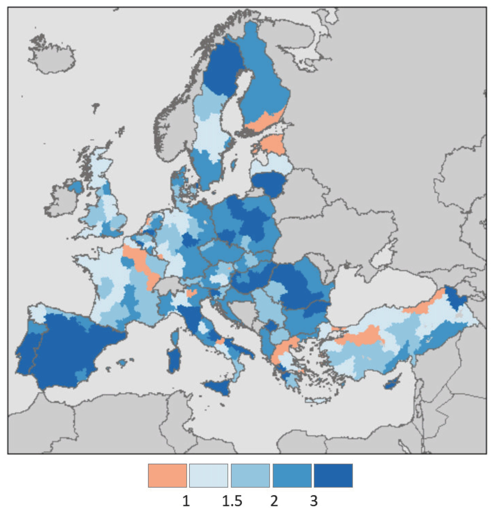
Figure 9Spatial distribution of the ratio between the number of fAPAR anomalies in the optimal period (see Sect. 3.3) during low-yield years (yield anomalies ) and other years (yield anomalies ).
Overall, values greater than 1 are observed over most of Europe in Fig. 9, suggesting a good performance of fAPAR anomalies to detect extreme low conditions in annual yield. While the ratio is only slightly higher than 1 in some regions where the previous analyses highlight poor performances (i.e. the UK and France), years with severe reductions in yield are still well captured by fAPAR.
Finally, the plot in Fig. 10 shows a comparison between the ratio computed on the optimal period (grey area) and the one computed on the full year (all 36 dekads, black area). Since the years are divided in the two categories based on yield data, the size of the two datasets is independent from the selected period (optimal or full year), making the intercomparison straightforward. The plot shows an overall increase in the ratio when only the dekads in the optimal period are considered, which translate to a better ability to discriminate low-yield years compared to simply accounting for all the anomalies observed across the full year.
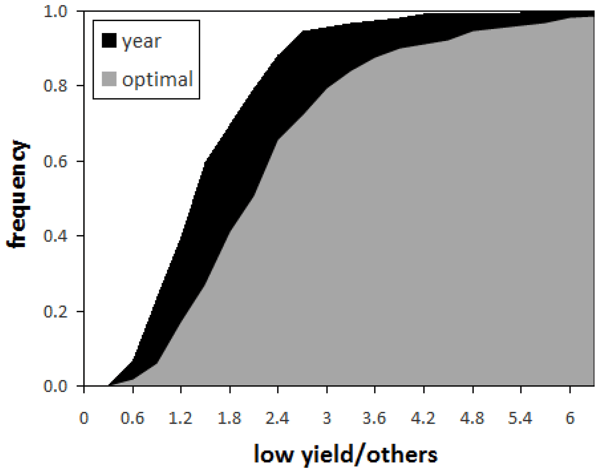
Figure 10Cumulated frequency of (i) the ratio between the number of fAPAR anomalies in the optimal period (see Sect. 3.3) during low-yield years (yield anomalies ) and other years (yield anomalies ) (optimal, grey area) and (ii) the ratio between the number of fAPAR anomalies in the full year (36 dekads) during low-yield years and other years (year, black area).
The value of the results reported in the previous section in the context of drought monitoring is related to the assumption that anomalies of cereal yields show the effects of drought on vegetation during drought years, as demonstrated, for example, by Brás et al. (2021), who quantified an approximately 9 % reduction in European cereal yields due to historical droughts (1961–2018), with an increasing intensity in more recent years. The spatial patterns in negative yield anomalies for the dataset used in this study, and the cross-comparison with documented past drought events, confirm the general assumption that low yields are recorded during drought years, even if not all the low yield values may be associated to droughts. These data confirm that understanding the role of fAPAR as proxy for yield is valuable for drought monitoring, even if a non-exclusive correspondence between low yield/fAPAR and drought exists.
Due to the focus on data commonly used in operational drought monitoring systems, a common element for all the performed analyses is the independent use of each dekadal fAPAR time series. While different results may be achieved by using metrics based on the full growing season (e.g. Kang et al., 2018), such analyses are not easily transferable to a near-real-time monitoring framework. Overall, the correlation coefficients computed using fAPAR collected during multiple dekads suggest a predominance of positive values over all regions. This is in line with the expected direct relationship between fAPAR and yield during the core growing season, as well as with most of the past studies which focused primarily on the positive correlation. Indeed, most of the maximum values of correlation seems to be located within the conventional growing season, and the south–north gradient observed in both of the positive homogeneous period maps (Fig. 3) is in broad agreement with the expected increasing gradient in growing season length observed over Europe (Rötzer and Chmielewski, 2001). However, there is not a perfect matching between the growing seasons and the periods with higher correlation values, and while studies on satellite-derived phenology have detected growing season lengths ranging from 5 to 9 months (Rötzer and Chmielewski, 2001), the average length of the periods with positive and statistically significant correlations seems to be shorter.
Consistently high positive correlation values are obtained over most of Spain, in line with a recent study over the region (García-León et al., 2019), which reported good performances of the satellite-based vegetation condition index (VCI) for different types of cereals, especially for winter wheat and barley. Over central Italy, Todisco et al. (2008) observed good correlation between yield in sunflower and sorghum with common drought indices (standardized precipitation index, SPI; and soil moisture severity index), with a maximum correlation around weeks 27–29 of the growing season (i.e. July) and statistically significant values for periods ranging from 2 to 4 months. Similar timing, but with a slightly shorter optimal length, has been observed in our analysis for the same area.
For Germany, Bachmair et al. (2018) found significant correlation values between VCI and vegetation health index (VHI) anomalies in the month of August, and yield deviations for maize, that are comparable with the maximum values observed for western Germany in our study. A mix of high correlation and missing data is reported in that study for eastern Germany, where our results are statistically significant only for a very limited period. These differences may be explained by the focus on specific crop types (not included in our study), as the same authors also highlight how the accuracy of their relationships varied for the different crops.
Similar to our results, Labudová et al. (2017) found significant correlation with SPI and standardized precipitation evapotranspiration index (SPEI) in the Danubian lowlands only for summer months, or for a very limited time (i.e. June) in the eastern Slovak lowlands. For these regions, the values of the maximum homogeneous period with ranged between 3 and 9 dekads as shown in Fig. 3.
The good results observed over the western Mediterranean and the countries around the Black Sea are in agreement with the findings of López-Lozano et al. (2015), who reported a similar pattern in their study based on a different fAPAR product (derived from another satellite sensor). This seems to suggest that the observed relationship is likely independent from the data source and more intrinsically connected to the capability of the physical quantity fAPAR to reflect the variation in yield under certain conditions.
The presence of limited periods with consecutive negative correlations early in the growing season may be related to the lagged response of vegetation to water deficits (Crow et al., 2012), which results in positive greenness anomalies early in the season followed by negative values later on (i.e. delay in the phenological cycle). Another explanation can be the limited immediate effect of water deficit during energy-limited periods (Zscheischler et al., 2015), which can also be the reason behind the general poor correlation between fAPAR and yield over regions where water is not a key limiting factor. This inverse relationship observed early in the season is currently under-explored in drought monitoring systems, which mostly focus on the direct relationship, and it may have an interesting role as an early warning tool under specific conditions. However, the results obtained in this study suggest a limited temporal extension and statistical robustness of the periods with inverse relationships, which are usually followed by much longer and robust periods of direct relationship.
The late start of the optimal period in many regions of the Mediterranean and western Europe, compared to the rest of the domain, is associated with the presence of these periods of inverse relationship early in the growing season. Given the particular climate of the Mediterranean region and the key role of dry and hot spring–summer months in propagating the water deficits in the area, a lagged response in vegetation is expected. In contrast, central Europe is characterised by an earlier start of the optimal period (March to August) compared to the Mediterranean and western Europe that seems to precede the expected growing season (June to October), further stressing the imperfect match between optimal period and growing season. For central Europe, Potopová et al. (2015) found a high yield–drought correlation for cereals (better than other crops) over Czech Republic between April–June, a result in line with our findings. The late start (April/May) in the northern regions of Scandinavia compared to central Europe is mostly explained by the lack of reliable fAPAR data earlier in the year due to low sun angles.
Focusing on the optimal period, mixed performances are obtained in Italy, with low agreement particularly in Sardinia and regions along the Apennine mountains. Although García-León et al. (2021) found a positive relationship between annually cumulated fAPAR anomalies and yield for most main crop types, the aggregation of the results at national scale does not allow the detection of differences among regions. Given the complex morphology of those regions, potential unreliability in the fAPAR estimates may be a possible cause for the poor performances. Complex morphology can also be the reason for poor results over a few other Mediterranean areas, such as Greece.
The spatial variability of the dependence of yield on water-limiting factors can be one of the explanations for the observed patterns, with a stronger correlation between fAPAR and yield over water-limited regions (Zampieri et al., 2017) and weaker relationships over regions where other factors may play a major role in controlling yield rather than simply greenness dynamics. Similar considerations were also made by López-Lozano et al. (2015), even when results are disentangled between different crop types (wheat, barley, and maize).
Indeed, another possible contributing factor underlying the spatial differences in the retrieved optimal periods can be the potentially variable responses of different cereal types included within the overall cereals Eurostat category. Since different predominant cereal types are cultivated locally, this variability can also contribute to the observed spatial variability in the results. This is supported by other studies that have demonstrated different responses for different crop types (García-León et al., 2021; Labudová et al., 2017). While applying the analysis to different cereal subcategories, or even different plant types, may be useful to better understand the relationship between fAPAR and yield for each specific crop, the results of this study for all cereals provide valuable experimental information on optimal periods that can be more easily integrated into an operational drought monitoring system, which focuses not only on agricultural drought impacts.
In this study, records of annual crop yield data for cereals were used to evaluate the performance of satellite-derived fAPAR time series data in capturing year-by-year variations in crop production for different periods of the year and growth stages of vegetation, given that fAPAR anomalies (or other greenness indices) are often used in drought studies to capture the effect of drought events on vegetation in the absence of yield data.
Overall, the analysis of the correlograms computed by plotting anomalies of dekadal fAPAR values against yearly yield deviations was used for three main purposes:
-
investigation of continuous streaks of dekads with homogeneous behaviour (direct vs. inverse) and agreement (i.e. statistical significance) but with different temporal length,
-
investigation of fixed-length (6 to 8 months) optimal periods, defined as the function of the maximum average r within the given range of lengths, and
-
evaluation of the capability of fAPAR anomalies during the optimal periods to discriminate between low-yield and other years.
The analyses confirm the period of March to October as being the most relevant to positively correlate anomalies of fAPAR and crop yield, being the period when most of the highest values of correlation are estimated and when most of the continuous periods with statistically significant and positive r values are located. There is generally a good agreement between these findings and both the duration and temporal location of the commonly defined growing seasons in Europe, even if spatial patterns in periods with positive correlations and growing season can also be rather different. While some periods with consistent negative correlations are also observed between February and May, these are generally too limited in length to be considered a primary source of information to reproduce yield dynamics, but they have potential as valuable early warning information sources.
The average growing period in Europe is usually characterised by a marked south-to-north gradient, which is also observed in our analysis of the 6- to 8-month optimal periods based on average r values. Some clear spatial patterns emerge in this analysis, such as the early start in most of central Europe and the southern Mediterranean, as well as the late start in southern and western Europe. These spatial patterns do not exactly match commonly observed satellite-derived growing seasons, so they provide an independent assessment of which phases of the phenological cycle are more valuable to capture yield variations – valuable information that can be incorporated into operational drought monitoring systems.
Another key output of the study is the generally good correlation between fAPAR anomalies and crop yield anomalies over most of the Mediterranean regions and across the full range of variability of yield data. This result can be explained by the strong dependency of both yield and vegetation greenness on water-limiting factors, as also suggested by López-Lozano et al. (2015) and Zampieri et al. (2017). Given the well-documented high vulnerability of this region to drought and the increasing threat posed by climate change (Cammalleri et al., 2020; Dubrovský et al., 2014), this result suggests the possibility to link satellite-observed fAPAR anomalies with actual impacts in agriculture, as a promising new development that merits further exploration.
This study also highlights the overall limited correlation, outside of very short time periods, between fAPAR and yield over most of the NUTS 2 regions in central Europe. Further analyses may be needed to better understand the reason behind this result. In this context, a recent study by Beillouin et al. (2020) has demonstrated how simple climate variables (i.e. high temperature and low precipitation) can explain much of the yield variability in central Europe, in contrast with the situation in southern Europe. It is important to further remark that even over these regions where the overall performance is limited, fAPAR anomalies are still successful in discriminating between low-yield years and the rest, which is still a relevant feature to be further exploited in drought monitoring systems.
The fAPAR dataset used in this study can be retrieved from the Joint Research Centre Data Catalogue at http://data.europa.eu/89h/91a222a0-74fe-468f-b53a-b622aa1161cf (EDO, 2021).
CC designed the experiments with inputs from AT and NMC. CC developed the codes and performed the analyses. CC prepared the paper with contributions and revisions from all co-authors.
The contact author has declared that none of the authors has any competing interests.
Publisher's note: Copernicus Publications remains neutral with regard to jurisdictional claims in published maps and institutional affiliations.
This paper was edited by Brunella Bonaccorso and reviewed by Marthe Wens and one anonymous referee.
Atzberger, C., Klisch, A., Mattiuzzi, M., and Vuolo, F.: Phenological metrics derived over the European continent from NDVI3g data and MODIS time series, Remote Sens.-Basel, 6, 257–284, https://doi.org/10.3390/rs6010257, 2014.
Bachmair, S., Tanguy, M., Hannaford, J., and Stahl, K.: How well do meteorological indicators represent agricultural and forest drought across Europe?, Environ. Res. Lett., 13, 034042, https://doi.org/10.1088/1748-9326/aaafda, 2018.
Barros, J. R. A., Guimaraes, M. J. M., Simões, W. L., de Melo, N. F., and Angelotti, F.: Water restriction in different phenological stages and increased temperature affect cowpea production, Agr. Sci., 45, 1–12, https://doi.org/10.1590/1413-7054202145022120, 2021.
Beillouin, D., Schauberger, B., Bastos, A., Ciais, P., and Makowski, D.: Impact of extreme weather conditions on European crop production in 2018, Philos. T. Roy. Soc. B, 375, 20190510, https://doi.org/10.1098/rstb.2019.0510, 2020.
Bogdan, O., Marinică, I., and Mic, L.-E.: Characteristics of the summer drought 2007 in Romania, Proceedings of the 2008 BALWOIS Conference, 27–31 May 2008, Ohrid, Republic of Macedonia, http://balwois.com/wp-content/uploads/old_proc/ffp-1075.pdf (last access: July 2021), 2008.
Brás, T. A., Seixas, J., Carvalhais, N., and Jägermeyr, J.: Severity of drought and heatwave crop losses tripled over the last five decades in Europe, Environ. Res. Lett., 16, 065012, https://doi.org/10.1088/1748-9326/abf004, 2021.
Brown, R. G. and Meyer, R. F.: The fundamental theory of exponential smoothing, Oper. Res., 9, 673–685, https://doi.org/10.1287/opre.9.5.673, 1961.
Buras, A., Rammig, A., and Zang, C. S.: Quantifying impacts of the 2018 drought on European ecosystems in comparison to 2003, Biogeosciences, 17, 1655–1672, https://doi.org/10.5194/bg-17-1655-2020, 2020.
Cammalleri, C., Naumann, G., Mentaschi, L., Bisselink, B., Gelati, E., De Roo, A., and Feyen, L.: Diverging hydrological drought traits over Europe with global warming, Hydrol. Earth Syst. Sci., 24, 5919–5935, https://doi.org/10.5194/hess-24-5919-2020, 2020.
Ceglar, A., Toreti, A., Zampieri, M., Manstretta, V., Bettati, T., and Bratu, M.: Clisagri: An R package for agro-climate services, Climate Serv., 20, 100197, https://doi.org/10.1016/j.cliser.2020.100197, 2020.
Chaves, M. M., Pereira, J. S., Maroco, J., Rodrigues, M. L., Ricardo, C. P. P., Osório, M. L., Carvalho, I., Faria, T., and Pinheiro, C.: How Plants Cope with Water Stress in the Field?, Photosynthesis and Growth, Ann. Bot.-London, 89, 907–916, https://doi.org/10.1093/aob/mcf105, 2002.
Crow, W. T., Kumar, S. V., and Bolten, J. D.: On the utility of land surface models for agricultural drought monitoring, Hydrol. Earth Syst. Sci., 16, 3451–3460, https://doi.org/10.5194/hess-16-3451-2012, 2012.
De Bono, A., Peduzzi, P., Kluser, S., Giuliani, G., and United Nations Environment Programme: Impacts of Summer 2003 Heat Wave in Europe, Environment Alert Bulletin, 2, 4, http://archive-ouverte.unige.ch/unige:32255 (last access: September 2022), 2004.
Demirevska, K., Zasheva, D., Dimitrov, R., Simova-Stoilova, L., Stamenova, M., and Feller, U.: Drought stress effects on Rubisco in wheat: changes in the Rubisco large subunit, Acta Physiol. Plant., 31, 1129–1138, https://doi.org/10.1007/s11738-009-0331-2, 2009.
Demuth, S.: Learning to live with drought in Europe, A World of Science, 7, 18–20, https://www.geo.uio.no/edc/downloads/ (last access: October 2022), 2009.
Dubrovský, M., Hayes, M., Duce, P., Trnka, M., Svoboda, M., and Zara, P.: Multi-GCM projections of future drought and climate variability indicators for the Mediterranean region, Reg. Environ. Change, 14, 1907–1919, https://doi.org/10.1007/s10113-013-0562-z, 2014.
EDO – European Drought Observatory: EDO Fraction of Absorbed Photosynthetically Active Radiation (FAPAR) Anomaly (MODIS) (version 1.3.2), European Commission, Joint Research Centre (JRC) [data set], http://data.europa.eu/89h/91a222a0-74fe-468f-b53a-b622aa1161cf (last access: Novmeber 2022), 2021.
Eurostat: Annual crop statistics: Handbook 2020 edition, 167 pp., https://ec.europa.eu/eurostat/cache/metadata/Annexes/apro_cp_esms_an1.pdf (last access: July 2021), 2020.
FAO – Food and Agriculture Organization of the United Nations: The impact of natural hazards and disasters on agriculture and food security and nutrition: A call for action to build resilient livelihoods, Rome, Italy, 16 pp., http://www.fao.org/3/i4434e/i4434e.pdf (last access: July 2021), 2015.
FAO – Food and Agriculture Organization of the United Nations: The impact of disasters and crises on agriculture and food security: 2021, Rome, Italy, 245 pp., https://doi.org/10.4060/cb3673en (last access: September 2022), 2021.
FAO – Food and Agriculture Organization of the United Nations, IFAD – International Fund for Agricultural Development, UNICEF – United Nations Children's Fund, WFP – World Food Programme, and WHO – World Health Organization: The State of Food Security and Nutrition in the World 2018, Building climate resilience for food security and nutrition, Rome, Italy, 202 pp., https://www.fao.org/3/I9553EN/i9553en.pdf (last access: December 2021), 2018.
García-Herrera, R., Paredes, D., Trigo, R. M., Trigo, I. F., Hernandez, H., Barriopedro, D., and Mendes, M. T.: The outstanding 2004–2005 drought in the Iberian Peninsula: associated atmospheric circulation, J. Hydrometeorol., 8, 483–498, https://doi.org/10.1175/JHM578.1, 2007.
García-Herrera, R., Garrido-Perez, J. M., Barriopedro, D., Ordóñez, C., Vicente-Serrano, S. M., Nieto, R., Gimeno, L., Sorí, R., and Yiou, P.: The European 2016/17 Drought, J. Climate, 32, 3169–3187, https://doi.org/10.1175/JCLI-D-18-0331.1, 2019.
García-León, D., Contreras, S., and Hunink, J.: Comparison of meteorological and satellite-based indices as yield predictors of Spanish cereals, Agr. Water Manage., 213, 388–396, https://doi.org/10.1016/j.agwat.2018.10.030, 2019.
García-León, D., Standardi, G., and Staccione, A.: An integrated approach for the estimation of agricultural drought costs, Land Use Policy, 100, 104923, https://doi.org/10.1016/j.landusepol.2020.104923, 2021.
Gouveia, C., Trigo, R. M., and DaCamara, C. C.: Drought and vegetation stress monitoring in Portugal using satellite data, Nat. Hazards Earth Syst. Sci., 9, 185–195, https://doi.org/10.5194/nhess-9-185-2009, 2009.
Kang, W., Wang, T., and Liu, S.: The response of vegetation phenology and productivity to drought in semi-arid regions of northern China, Remote Sens.-Basel, 10, 727, https://doi.org/10.3390/rs10050727, 2018.
Knyazikhin, Y., Martonchik, Y. V., Myneni, R. B., Diner, D. J., and Running, S. W.: Synergistic algorithm for estimating vegetation canopy leaf area index and fraction of absorbed photosynthetically active radiation from MODIS and MISR Data, J. Geophys. Res., 103, 32257–32274, https://doi.org/10.1029/98JD02462, 1998.
Labudová, L., Labuda, M., and Takáč, J.: Comparison of SPI and SPEI applicability for drought impact assessment on crop production in the Danubian lowland and the East Slovakian lowland, Theor. Appl. Climatol., 128, 491–506, https://doi.org/10.1007/s00704-016-1870-2, 2017.
López-Lozano, R., Duveiller, G., Seguini, L., Meroni, M., García-Condado, S., Hooker, J., Leo, O., and Baruth, B.: Towards regional grain yield forecasting with 1km-resolution EO biophysical products: Strengths and limitations at pan-European level, Agric. Forest Meteorol., 206, 12–32, https://doi.org/10.1016/j.agrformet.2015.02.021, 2015.
Monteleone, B., Borzí, I., Bonaccorso, B., and Martina, M.: Developing stage-specific drought vulnerability curves for maize: The case study of the Po River basin, Agr. Water Manage., 269, 107713, https://doi.org/10.1016/j.agwat.2022.107713, 2022.
Myneni, R. B.: MOD15A2H MODIS/Terra Leaf Area Index/FPAR 8-Day L4 Global 500 m SIN Grid V006, NASA EOSDIS Land Processes DAAC, https://doi.org/10.5067/modis/mod15a2h.006, 2015.
Potopová, V., Štepánek, P., Možný, M., Turoktt, L., and Soukup, J.: Performance of the standardized precipitation evapotranspiration index at various lags for agricultural drought risk assessment in the Czech Republic, Agric. Forest Meteorol., 202, 26–38, https://doi.org/10.1016/j.agrformet.2014.11.022, 2015.
Rebetez, M., Mayer, H., Dupont, O., Schindler, D., Gartner, K., Kropp, J. P., and Menzel, A.: Heat and drought 2003 in Europe: A climate synthesis, Ann. For. Sci., 63, 569–577, https://doi.org/10.1051/forest:2006043, 2006.
Rembold, F., Meroni, M., Urbano, F., Csak, G., Kerdiles, H., Perez-Hoyos, A., Lemoine, G., Leo, O., and Negre, T.: ASAP: A new global early warning system to detect anomaly hot spots of agricultural production for food security analysis, Agr. Syst., 168, 247–257, https://doi.org/10.1016/j.agsy.2018.07.002, 2019.
Rojas, O., Vrieling, A., and Rembold, F.: Assessing drought probability for agricultural areas in Africa with coarse resolution remote sensing imagery, Remote Sens. Environ., 115, 343–352, https://doi.org/10.1016/j.rse.2010.09.006, 2011.
Rossi, S., Weissteiner, C., Laguardia, G., Kurnik, B., Robustelli, M., Niemeyer, S., and Gobron, N.: Potential of MERIS fAPAR for drought detection, in: Proceedings of the 2nd MERIS/(A)ATSR User Workshop, ESA SP-666, edited by: Lacoste, H. and Ouwehand, L., 6. Frascati, Italy, ESA Communication Production Office, https://www.researchgate.net/profile/Christof-Weissteiner/publication/228417050_Potential_of_MERIS_fAPAR_for_drought_detection/links/00b49518362dcb5b6d000000/Potential-of-MERIS-fAPAR-for-drought-detection.pdf (last access: November 2022), 2008.
Rötzer, T. and Chmielewski, F. M.: Phenological maps of Europe, Clim. Res., 18, 249–257, https://doi.org/10.3354/cr018249, 2001.
Sassenrath, G. F., Schneider, J. M., Gaj, R., Grzebisz, W., and Halloran, J. M.: Nitrogen balance as an indicator of environmental impact: Toward sustainable agricultural production, Renew. Agr. Food Syst., 28, 276–289, https://doi.org/10.1017/S1742170512000166, 2012.
Sima, M., Popovici, E.-A., Bălteanu, D., Micu, D. A., Kucsicsa, G., Dragotă, C., and Grigorescu, I.: A farmer-based analysis of climate change adaptation options of agriculture in the Bărăgan Plain, Romania, Earth Perspect., 2, 5, https://doi.org/10.1186/s40322-015-0031-6, 2015.
Somorowska, U.: Changes in drought conditions in Poland over the past 60 years evaluated by the Standardized Precipitation-Evapotranspiration Index, Acta Geophys., 64, 2530–2549, https://doi.org/10.1515/acgeo-2016-0110, 2016.
Spinoni, J., Naumann, G., Vogt, J. V., and Barbosa, P.: The biggest drought events in Europe from 1950 to 2012, J. Hydrol. Reg. Studies, 3, 509–524, https://doi.org/10.1016/j.ejrh.2015.01.001, 2015.
Stahl, K., Kohn, I., Blauhut, V., Urquijo, J., De Stefano, L., Acácio, V., Dias, S., Stagge, J. H., Tallaksen, L. M., Kampragou, E., Van Loon, A. F., Barker, L. J., Melsen, L. A., Bifulco, C., Musolino, D., de Carli, A., Massarutto, A., Assimacopoulos, D., and Van Lanen, H. A. J.: Impacts of European drought events: insights from an international database of text-based reports, Nat. Hazards Earth Syst. Sci., 16, 801–819, https://doi.org/10.5194/nhess-16-801-2016, 2016.
Stallmann, J., Schweiger, R., Pons, C. A. A., and Müller, C.: Wheat growth, applied water use efficiency and flag leaf metabolome under continuous and pulsed deficit irrigation, Sci. Rep.-UK, 10, 10112, https://doi.org/10.1038/s41598-020-66812-1, 2020.
Tadesse, T., Senay, G. B., Berhan, G., Regassa, T., and Beyene, S.: Evaluating a satellite-based seasonal evapotranspiration product and identifying its relationship with other satellite-derived products and crop yield: a case study for Ethiopia, Int. J. Appl. Earth Obs., 40, 39–54, https://doi.org/10.1016/j.jag.2015.03.006, 2015.
Todisco, F., Vergni, L., and Mannocchi, F.: An evaluation of some drought indices in the monitoring and prediction of agricultural drought impact in central Italy, in: Irrigation in Mediterranean agriculture: challenges and innovation for the next decades, edited by: Santini, A., Lamaddalena, N., Severino, G., and Palladino, M., CIHEAM, Bari, 2008, 203–211, Options Méditerranéennes: Série A, Séminaires Méditerranéens, no. 84, http://om.ciheam.org/article.php?IDPDF=800967 (last access: July 2021), 2008.
Toreti, A., Belward, A., Perez-Dominguez, I., Naumann, G., Luterbacher, J., Cronie, O., Seguini, L., Manfron, G., Lopez-Lozano, R., Baruth, B., van den Berg, M., Dentener, F., Ceglar, A., Chatzopoulos, T., and Zampieri, M.: The Exceptional 2018 European Water Seesaw Calls for Action on Adaptation, Earths Future, 7, 652–663, https://doi.org/10.1029/2019EF001170, 2018.
United Nations Office for Disaster Risk Reduction: GAR Special Report on Drought 2021, Geneva, 210 pp., ISBN 9789212320274, https://www.undrr.org/publication/gar-special-report-drought-2021, last access: July 2021.
Valiukas, D.: Analysis of droughts and dry periods in Lithuania. Summary of Doctoral Dissertation, Vilnius University, 49 pp., https://epublications.vu.lt/object/elaba:8754330 (last access: July 2021), 2015.
van Hateren, T. C., Chini, M., Matgen, P., and Teuling, A. J.: Ambiguous agricultural drought: Characterising soil moisture and vegetation droughts in Europe from earth observation, Remote Sens.-Basel, 13, 1990, https://doi.org/10.3390/rs13101990, 2021.
Vicente-Serrano, S. M., Beguería, S., Lorenzo-Lacruz, J., Camarero, J. J., López-Moreno, J. I., Azorin-Molina, C., Revuelto, J., Morán-Tejeda, E., and Sanchez-Lorenzo, A.: Performance of drought indices for ecological, agricultural, and hydrological applications, Earth Interact., 16, 1–27, https://doi.org/10.1175/2012EI000434.1, 2012.
Wang, Y., Tian, Y., Zhang, Y., El-Saleous, N., Knyazikhin, Y., Vermote, E., and Myneni, R. B.: Investigation of product accuracy as a function of input and model uncertainties: Case study with SeaWiFS and MODIS LAI/FPAR algorithm, Remote Sens. Environ., 78, 296–311, https://doi.org/10.1016/S0034-4257(01)00225-5, 2001.
WMO – World Meteorological Organization and GWP – Global Water Partnership: Handbook of Drought Indicators and Indices, edited by: Svoboda, M. and Fuchs, B. A., Integrated Drought Management Programme (IDMP), Integrated Drought Management Tools and Guidelines Series 2, Geneva, 53 pp., ISBN 978-92-63-11173-9, 2016.
Yang, J., Wu, J., Liu, L., Zhou, H., Gong, A., Han, X., and Zhao, W.: Response of winter wheat to drought in the north China plain: spatial-temporal patterns and climate drivers, Water, 12, 3094, https://doi.org/10.3390/w12113094, 2020.
Zampieri, M., Ceglar, A., Dentener, F., and Toreti, A.: Wheat yield loss attributable to heat waves, drought and water excess at the global, national and subnational scales, Environ. Res. Lett., 12, 064008, https://doi.org/10.1088/1748-9326/aa723b, 2017.
Zscheischler, J., Orth, R., and Seneviratne, S. I.: A submonthly database for detecting changes in vegetation-atmosphere coupling, Geophys. Res. Lett., 42, 9816–9824, https://doi.org/10.1002/2015GL066563, 2015.