the Creative Commons Attribution 4.0 License.
the Creative Commons Attribution 4.0 License.
 | 22 Aug 2022
The impact of terrain model source and resolution on snow avalanche modeling
Pascal Sirguey
Simon Morris
Perry Bartelt
Nicolas Cullen
Todd Redpath
Kevin Thompson
Yves Bühler
Natural hazard models need accurate digital elevation models (DEMs) to simulate mass movements on real-world terrain. A variety of platforms (terrestrial, drones, aerial, satellite) and sensor technologies (photogrammetry, lidar, interferometric synthetic aperture radar) are used to generate DEMs at a range of spatial resolutions with varying accuracy. As the availability of high-resolution DEMs continues to increase and the cost to produce DEMs continues to fall, hazard modelers must often choose which DEM to use for their modeling. We use satellite photogrammetry and topographic lidar to generate high-resolution DEMs and test the sensitivity of the Rapid Mass Movement Simulation (RAMMS) software to the DEM source and spatial resolution when simulating a large and complex snow avalanche along Milford Road in Aotearoa/New Zealand. Holding the RAMMS parameters constant while adjusting the source and spatial resolution of the DEM reveals how differences in terrain representation between the satellite photogrammetry and topographic lidar DEMs (2 m spatial resolution) affect the reliability of the simulation estimates (e.g., maximum core velocity, powder pressure, runout length, final debris pattern). At the same time, coarser representations of the terrain (5 and 15 m spatial resolution) simulate avalanches that run too far and produce a powder cloud that is too large, though with lower maximum impact pressures, compared to the actual event. The complex nature of the alpine terrain in the avalanche path (steep, rough, rock faces, treeless) makes it a suitable location to specifically test the model sensitivity to digital surface models (DSMs) where both ground and above-ground features on the topography are included in the elevation model. Considering the nature of the snowpack in the path (warm, deep with a steep elevation gradient) lying on a bedrock surface and plunging over a cliff, RAMMS performed well in the challenging conditions when using the high-resolution 2 m lidar DSM, with 99 % of the simulated debris volume located in the documented debris area.
- Article
(17946 KB) - Full-text XML
- BibTeX
- EndNote


Natural hazards like snow, ice and rock avalanches, debris flows, and landslides pose risk to people and infrastructure in alpine regions (Badoux et al., 2016; Techel et al., 2016; Dowling and Santi, 2013). While predicting the timing and destructive capacity of a natural hazard remains an unsolved challenge for researchers, the development of dynamic hazard models to anticipate potential impacts has provided a valuable risk-mitigation tool used in hazard mapping, in land planning, for engineering mitigation measures, and to reanalyze or back-calculate historic events (Bühler et al., 2022; Baggio et al., 2021; Christen et al., 2010a; Casteller et al., 2008). Natural hazard modeling of mass transport has evolved rapidly as the physics are better understood and detailed event observations are becoming more readily available for model calibration.
The early development of one-dimensional models (Bartelt et al., 1999; Salm, 1966; Voellmy, 1955) has evolved into more complex two-dimensional and three-dimensional numerical simulations. Some examples of models simulating gravity-driven flows on three-dimensional terrain include RAMMS (Rapid Mass Movement Simulation; Christen et al., 2010b), r.avaflow (Mergili, 2020; Mergili et al., 2017), DAN and DAN3D (Dynamic ANalysis Hungr and McDougall, 2009), Flow-R (Horton et al., 2013), SamosAT (Snow and Avalanche MOdelling and Simulation – Advanced Technology; Sampl and Zwinger, 2004), TRENT2D* (Zugliani and Rosatti, 2021), and others (van den Bout et al., 2021; Li et al., 2021; Rauter et al., 2018; Hergarten and Robl, 2015; Medina et al., 2008; Rickenmann et al., 2006). Dynamic models simulate flow characteristics on real-world topography, represented efficiently, but imperfectly, by a digital elevation model (DEM). The DEM is usually stored as a two-dimensional grid projected in a cartesian coordinate system, where each cell value is the height above a datum (Claessens et al., 2005; Wise, 2000; Gao, 1997). The technique of topographic data capture and processing, as well as the spatial resolution of the DEM, controls the level of detail achieved in elevation models. For instance, DEMs available at a global scale are coarser and miss fine-scale topography. Conversely, very-high-spatial-resolution DEMs can resolve fine-scale topography but are often limited to smaller spatial extents and impose higher computational requirements for the simulation.
In this context, hazard modelers must judge the most appropriate DEM for the study domain based on availability, cost, currency (the most recent or before/after an event altered a landscape), season (snow-on vs snow-off), completeness (whether data voids or holes exist the DEM), spatial resolution, accuracy, and whether the DEM is a digital terrain model (DTM) or digital surface model (DSM), subsets of the more generic DEM terminology. The choice of DEM will have implications for the influence of terrain features on flow characteristics, such as runout distance and channel overflowing for debris flows and rock avalanches (Zhao and Kowalski, 2020; Tarolli, 2014; Simoni et al., 2012; Allen et al., 2009), or runout distances, estimated maximum core velocities and impact pressures for snow avalanches (Bühler et al., 2011; Christen et al., 2010b). The effect and propagation of DEM uncertainties in model outputs (Zhao and Kowalski, 2020; Bühler et al., 2011) may be hard to identify and characterize without access to multiple DEM sources of variable accuracy. While higher-resolution DEMs are expected to represent terrain better, they may not always improve hazard modeling when used at their finest resolution as the model may be overly sensitive to fine-scale features in the case of landslide initiation and snow avalanches (Tarolli, 2014; Christen et al., 2010a). To best balance computational resources on the one hand and resolve appropriately scaled topography on the other, modelers often resample the DEM to a different spatial resolution from the source resolution. Upsampling a high-resolution DEM to a coarser grid size for hazard simulation may yield better results; however, downsampling to a lower-resolution DEM should be avoided (Bühler et al., 2011; Christen et al., 2010a).
1.1 Sensitivity of snow avalanche modeling to elevation product
The influence of spatial resolution on snow avalanche simulations has been studied previously (Brožová et al., 2021; Maggioni et al., 2013; Bühler et al., 2011; Christen et al., 2010a), establishing how a simulation is sensitive to the scale of terrain features resolved in the DEM. Morphometric measures of curvature, slope angle, aspect and roughness are all neighborhood functions applied to each cell where decreasing the resolution of the DEM will smooth large-scale terrain features and decrease the roughness of the surface (Brožová et al., 2021; Grohmann et al., 2011; Wu et al., 2008; Sappington et al., 2007; Kienzle, 2003; Gao, 1997; Bolstad and Stowe, 1994). Surface roughness controls friction between the dense core of the mass movement and the surface. Everything else being equal, both Brožová et al. (2021) and Bühler et al. (2011) demonstrated how increased roughness decreases the estimated runout of the dense core flow. Differences in simulations will be more pronounced in paths with confined terrain features such as gullies compared with broad open terrain. The rule of thumb has been to use a higher-spatial-resolution (as fine as 1 m) DEM for rough terrain and wet avalanches, while a coarser (up to 25 m) DEM is sufficient to capture relevant terrain features in smoother more homogeneous terrain, especially for large avalanche events (Bühler et al., 2011; Christen et al., 2010a).
When modeling snow avalanches, a DEM from a summer surface (snow-off) will represent terrain differently from a winter surface (snow-on). Maggioni et al. (2013) ran the same RAMMS simulations on 2 m summer and winter DEMs and found differences in runout length, deposition patterns and core velocities, attributable to different surface roughness in the paths, as well as the way confined terrain features in the summer surface were filled in with snow in the winter surface, in turn reducing roughness which resulted in debris spread over a wider area.
Furthermore, while not a problem for coarse global-scale DEMs, when using high-spatial-resolution DEMs it becomes important to distinguish between two subsets of the DEM, the digital surface model (DSM) and digital terrain model (DTM). A DSM includes above-ground terrain features such as shrubs, trees, and buildings and is the DEM product typically generated from optical photogrammetry and radar. A DTM distinguishes and removes these above-ground features from the bare-earth representation of the terrain. Based on the DEM capture technology, DTMs are obtained by morphological filtering of the DSM supplemented by direct retrieval of ground elevation below canopies, such as achieved by lidar (light detection and ranging). Depending on the point density, DTMs tend to exhibit smooth interpolation where above-ground points are removed. In regions with trees and shrubs a DTM may represent the terrain more smoothly with implications for hazard modeling.
Snow avalanches move over terrain differently depending on the type of avalanche (e.g., slab vs. loose, dry vs. wet), the snow temperature, the snow depth and snow-cover entrainment, among other factors. The use of a DTM creates a more realistic snow-covered surface that may better represent the sliding behavior of a slab avalanche immediately after release. A DSM may introduce unrealistic surface roughness in areas with trees and shrubs and other above-ground features, especially in the release zone; however, the DSM may better represent roughness in the track and runout where above-ground features provide more appropriate friction estimates (Brožová et al., 2021). In rocky alpine regions with few trees or shrubs, the DSM and DTM differences will be minor, and the higher roughness in the DSM may better reflect the terrain over which an avalanche runs.
1.2 State of elevation data products
The increased use of airborne and terrestrial lidar and optical sensors on RPAS (remotely piloted aircraft systems), airplanes and satellites offers accurate high-resolution (here we consider as 5 m spatial resolution or higher) elevation data at decreasing costs. At the same time projects like OpenTopography (Krishnan et al., 2011) improve data sharing and discovery. Advances in real-time global positioning and data processing workflows for large point cloud and image datasets have also helped generate more, and higher-quality, DEMs. However, most of these datasets exist as a patchwork, both spatially and temporally, with uneven distribution of high-resolution DEMs available globally and derived from a variety of remote sensing platforms and technologies. Many DEMs are generated at a project level or in response to a natural hazard rather than as part of a regional or national surveying program. They may have good relative accuracy but limited absolute accuracy, thus complicating their use with other datasets. Many alpine regions prone to natural hazards still lack a high-resolution DEM conforming to published accuracy standards. For example, the last national elevation product for Aotearoa/New Zealand was generated with aerial photogrammetry in the 1980s as 20 m contours and interpolated into a 15 m DEM (Columbus et al., 2011). Alpine regions may have episodic high-resolution data capture, but the rate of landscape change may render data rapidly obsolete. National programs for delivering standardized high-resolution DEMs exist in a number of countries facing alpine hazards (e.g., Canada, France, Aotearoa/New Zealand, Switzerland, United States), but baseline data delivery and renewal timeframes take years and may not prioritize alpine regions (e.g., Toitū Te Whenua/Land Information New Zealand, 2021).
Global DEM products (SRTM, ASTER, TanDEM-X, ALOS; see Rodríguez et al., 2006; Courty et al., 2019; Wessel et al., 2018; Takaku et al., 2014, respectively) suffer from the risk of data obsolescence and bring lower overall accuracy and potentially consequential artifacts for hazard modeling (Bühler et al., 2011). The EarthDEM product under development builds off the workflow for generating the ArcticDEM (Porter et al., 2018) and will leverage the archive of high-resolution imagery from the DigitalGlobe satellite constellation for 2 m DSM generation in regions across the globe. With the number of space-borne optical sensors continuing to increase, the use of high-resolution DSMs processed from stereo satellite images and multi-view imagery is also increasing.
1.2.1 Photogrammetry
Satellite photogrammetric mapping (SPM) uses two or more spatially overlapping digital images (classified as stereo, tri-stereo, multi-view) to generate a DSM. Clouds in an image will create data voids or holes in the DSM. Suitable sensor orientation and image contrast improve the DSM and must be considered when generating DSMs from satellite imagery in steep terrain or when the terrain is covered by snow (Eberhard et al., 2021; Shean et al., 2016). Nonetheless, SPM with images from a number of commercial sensors offers a large geographic extent (>400 km2) from a single acquisition capable of delivering a DSM resolution finer than 2 m with sub-meter vertical accuracy (Bhushan et al., 2021; Eberhard et al., 2021; Dehecq et al., 2020; Deschamps-Berger et al., 2020; Shean et al., 2016; Aguilar et al., 2014).
DSMs derived from digital images captured from an airplane and used in aerial photogrammetric mapping (APM) can be more highly resolved (0.5 m) and more accurate (0.15 m) than SPM-derived DSMs but at a higher cost and over a smaller spatial extent (Bühler et al., 2015; Nolan et al., 2015; Bühler et al., 2012). The development of RPAS photogrammetric mapping (RPM), which includes structure-from-motion photogrammetry workflows, produces very-high-resolution DSMs (0.05 m) that are as accurate as APM but over smaller spatial extents (1–5 km2 compared with 50–100 km2 for APM) and at a lower cost (Redpath et al., 2018; Bühler et al., 2016). Terrestrial photogrammetric mapping (TPM) has also been used to generate high-resolution DSMs (0.1 m) but with lower accuracy (0.5 m) and spatial extent (0.5–1 km2) as well as greater potential for obstructed terrain where no elevation estimates are generated (Eberhard et al., 2021; Prokop et al., 2015; Thibert et al., 2015).
1.2.2 Lidar
Light detection and ranging (lidar) often has the advantage of making more measurements per square meter than photogrammetry, depending on the distance between the sensor and the target. The higher measurement density and possibility of multiple returns through tree canopies allows for DTM generation more commonly than with photogrammetry. Lidar sensors are most common with aircraft and terrestrial laser scanners but are also increasingly available for use on a RPAS. Aerial laser scanning (ALS), either from an airplane or helicopter, typically achieves DEM resolutions of 0.5–1 m with a vertical accuracy of 0.1 m over a extent comparable to APM (50–100 km2) in a single campaign (Reutebuch et al., 2003). RPAS laser scanning (RLS) can generate DEM resolutions as high as 0.1 m and accuracy of 0.01 m over a slightly smaller spatial extent (0.2–0.5 km2) to RPM (Lassiter et al., 2021; Lin et al., 2019). Terrestrial laser scanning (TLS) can achieve very-high-resolution DEMs (0.05 m) with accuracy of 0.1 m and a wide range of spatial extents (0.5–5 km2) depending on the number of scanning positions and terrain (Prokop et al., 2015; Sommer et al., 2015; Deems et al., 2013). Although terrain obstruction may complicate capture, TLS can resolve complex shapes in the terrain, including steep and overhanging features that are not fully visible from above.
While aerial lidar is often considered the gold standard for topographic mapping and hazard modeling, offering both a high-resolution DTM and DSM over large geographic areas, ALS is expensive compared with other platforms (Bühler et al., 2012). Repeat ALS is useful for topographic change detection (Bernard et al., 2021; Booth et al., 2020), but rapid-response acquisitions after major events in remote alpine regions (e.g., Shugar et al., 2021) are often easier with SPM given acquisition logistics and data processing. An advantage for hazard modelers with access to terrestrial lidar is deployment immediately after an event to document landscape change (Bossi et al., 2015; Maggioni et al., 2013; Bartelt et al., 2012; Sovilla et al., 2010).
1.3 Goals of this study
Drawing from current recent advances in satellite photogrammetric mapping (SPM) and terrestrial laser scanning (TLS), we look at how differences in terrain representation influence snow avalanche hazard modeling. We simulate a large avalanche along Milford Road in Aotearoa/New Zealand using RAMMS to determine (1) the effects of topographic mapping technologies and (2) the influence of DSM resolution on simulation outputs. The unique combination of terrain (treeless, rough and steep) and snowpack characteristics (warm, dense and deep) in avalanche paths in Fiordland National Park provide suitable testing conditions to assess the role of terrain representation in the sensitivity of a dynamic hazard model.
After an overview of the study site, we explain the method for generating the DSMs. We then detail the well-documented avalanche event used in the RAMMS simulations, provide results from the simulations and show how different representations of terrain altered the simulated avalanche behavior. We then discuss the advantages and disadvantages of the elevation products for this type of simulation, with some lessons for dynamic hazard modeling more broadly.
1.4 Study site
The McPherson avalanche path is adjacent to State Highway 94 – Milford Road in Fiordland National Park, Aotearoa/New Zealand (Fig. 1). Milford Road connects Te Anau to Piopiotahi/Milford Sound, a popular tourist destination with an estimated 870 000 visitors in 2019 (Milford Opportunities Project, 2021). The highway crosses through alpine terrain and the Homer Tunnel at 927 m a.s.l., which had 300 000 vehicles pass through the tunnel in 2019 (Waka Kotahi/NZ Transport Agency, 2021). Homer Tunnel is located at the center of a 17 km stretch of highway with snow avalanche activity primarily affecting the road between June and December.
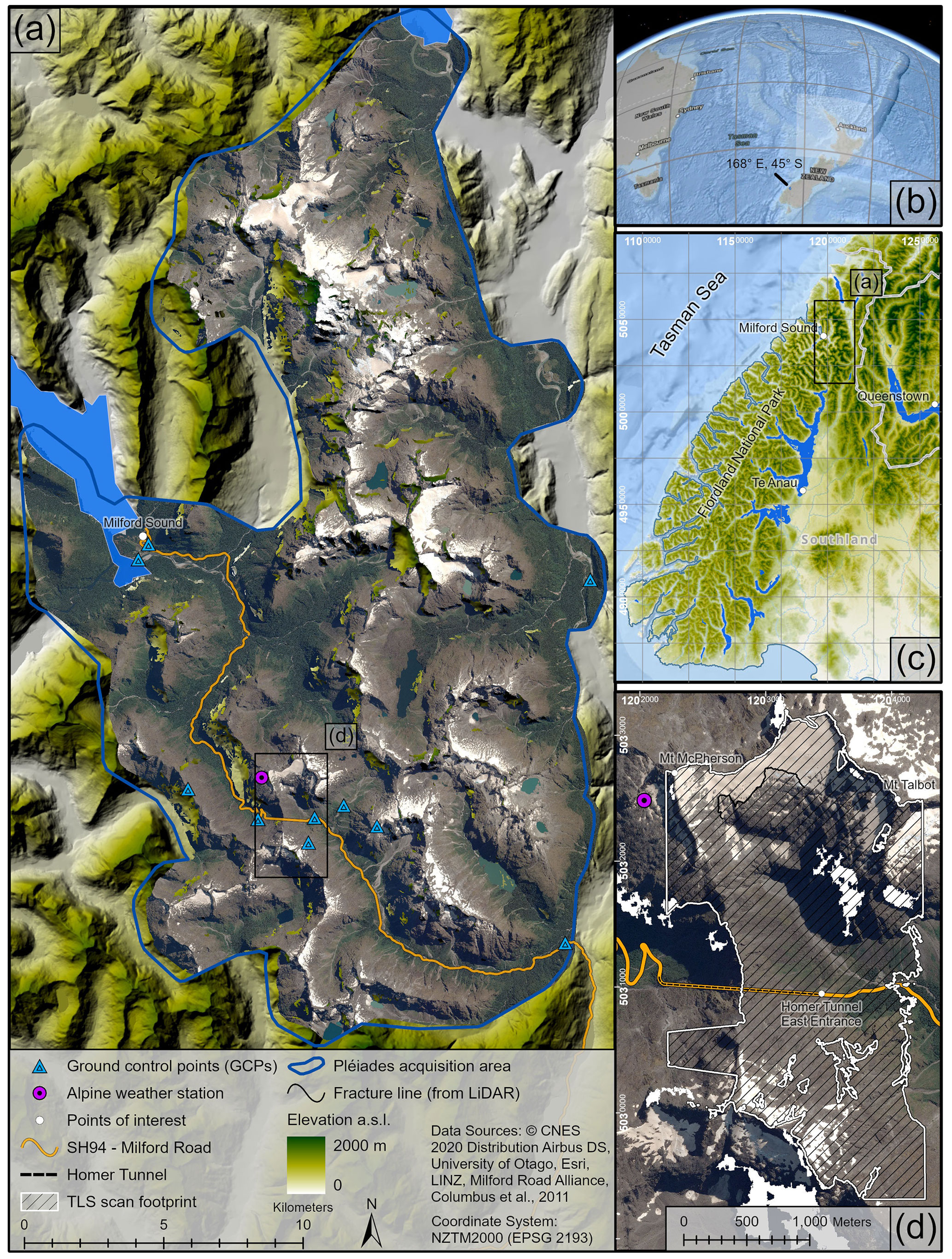
Figure 1Overview of study site with footprint of satellite imagery and location of ground control points (GCPs) in panel (a), reference maps in panels (b) and (c), and inset map showing the footprint of TLS data extent and McPherson 2020 avalanche fracture line in panel (d). SH94 Milford Road and the alpine weather station are also shown in panels (a) and (d).
1.4.1 Topography
Pleistocene glaciation in the Fiordland region of southwest Aotearoa/New Zealand carved deep valleys linking alpine regions with the Tasman Sea over short distances. Avalanche paths in Fiordland are characterized by large release zones, some with permanent snow, steep tracks with cliffs, and low-angle runout zones in u-shaped valleys. Avalanche paths have average slope angles of 30–35∘ with cliffs exceeding 75∘. The release zones range in size from 8000 to 860 000 m2 with an average of 100 000 m2 (Fitzharris and Owens, 1980). Some paths produce plunging avalanches because of the steep tracks (average slope over 50∘) where the core detaches from the terrain, landing again at the transition to lower-angle runout zones where they quickly lose momentum (Watson et al., 2021; Hendrikx, 2005; Schaerer, 1989; Fitzharris and Owens, 1980).
The geology of Fiordland has important implications for dynamic hazard modeling. The bedrock, predominantly Darran Complex in the study site (Bradshaw, 1990; Wood, 1960), consists primarily of relatively hard gabbro and hornblende diorite (Blattner, 1978). The surface topography in avalanche paths is characterized by little soil or vegetation and predominantly exposed bedrock. While avalanches run on bedrock in the tracks, paths often have loose rocks (scree) in the runout zones, which can be entrained in large avalanches. Regular plunging avalanches have also created tarns in some paths (Owens and Fitzharris, 1985) where the change in gradient between track and runout is most pronounced.
The McPherson avalanche path, the focus of this study, has a broad alpine release zone of approximately 60 000 m2 with a mean slope angle of 39∘ and primarily south-southeasterly aspect. It is approximately 10 km from Milford Sound and 25 km from the Tasman Sea (Fig. 1). The release zone has a mixture of permanent snow and exposed bedrock. The track begins with an over-steepened 150 m cliff, followed by a shelf and another 200 m cliff with slope angles exceeding 75∘, and is also comprised of bedrock with some scree. The runout is a valley comprised of rock and grasses with slope angles of 5–15∘ extending 1 km to Milford Road and the east portal of Homer Tunnel (Fig. 2). The only significant vegetation present in the path (besides alpine grasses and sparse shrubs in the runout) is trees located at the bottom of the path across Milford Road. There is no documentation of the avalanche core reaching the trees; however, the powder cloud from a McPherson avalanche in 2004 broke trees at the lowest point in the path. Since comprehensive record-keeping began in 1985, there have been 12 size 5 McPherson avalanches recorded, half of which were naturally released and half of which were released with active control.
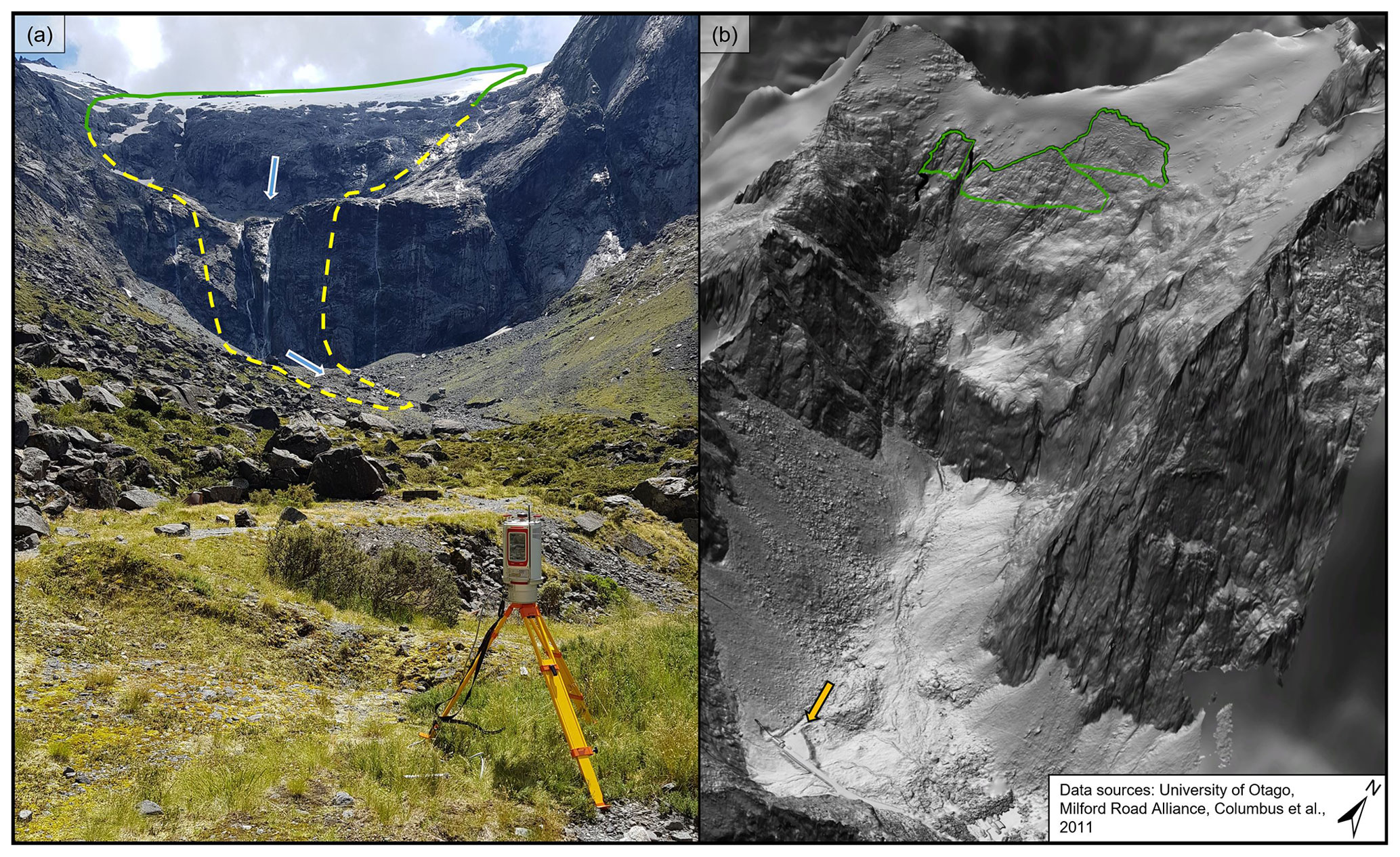
Figure 2Panel (a) shows the McPherson path in summer. The approximate delineation of the release area in green and track in yellow, with the Riegl VZ-6000 terrestrial laser scanner used in the study shown in the foreground. Homer Tunnel and Milford Road are located behind the camera. Picture courtesy of Downer Ltd. Milford Road Alliance. Panel (b) shows the full-resolution 0.5 m DSM hillshade draped on top of the 15 m NZSoSDEM hillshade, with the release areas in green and the location of the scanner in panel (a) shown with an arrow. To view the study site and model results in an interactive map, see Mountain Research Centre (2022).
1.4.2 Climatic setting
The Fiordland region has a maritime climate. Moisture laden air masses originating in the western half of the Tasman Sea are intercepted by high-relief coastal mountain ranges. The highest peak in the road corridor is Mt Christina (2474 m). This topographic barrier results in substantial orographic enhancement of precipitation. Maximum precipitation rates occur along the coast with a strong eastward precipitation gradient. Mean annual precipitation was 6716 mm at Milford Sound compared with 757 mm at Queenstown Airport (75 km to southeast) over the period 1981–2010 (Macara, 2015, 2013). The mean annual precipitation at the East Homer weather station adjacent to Milford Road (874 m a.s.l.) was over 6209 mm over the period 2011–2020. Over the same period the mean precipitation over the avalanche season (May to December) was 3703 mm. The mean annual air temperature was 6.3 ∘C, over the periods of 1993–2003 and 2010–2020, with a mean avalanche season air temperature of 3.7 ∘C. The mean air temperature at Cleddau weather station (1710 m a.s.l., Fig. 1) was 1.8 ∘C over the period of 2018–2020, with a mean avalanche season air temperature of −0.1 ∘C. The mean avalanche season air temperature at Cleddau indicates a mean seasonal freezing level of around 1700 m a.s.l.
This section discusses the data capture and processing workflows for generating DSMs (2, 5, 15 m) from satellite photogrammetric mapping (SPM) using a Pléiades satellite stereo pair and DSMs (0.5, 1, 2, 5, 15 m) from topographic lidar using Riegl VZ-6000 terrestrial laser scans. We used the best-available elevation data products for the region, in terms of accuracy and spatial resolution. We also included the highest-resolution nationwide DEM (Columbus et al., 2011) generated from 20 m contours derived in 1988 as part of the last national topographic survey using manual analogue photogrammetry. We included the full-resolution 15 m NZSoSDEM as well as a downsampled 5 m version for use in RAMMS. For more information on the state of elevation products in Aotearoa/New Zealand and globally, see Sect. 1.2. This section then details a case study of snow avalanche modeling used to highlight the sensitivity of the dynamic model to topographic representation. Figure 3 details the key processing steps in the workflow.
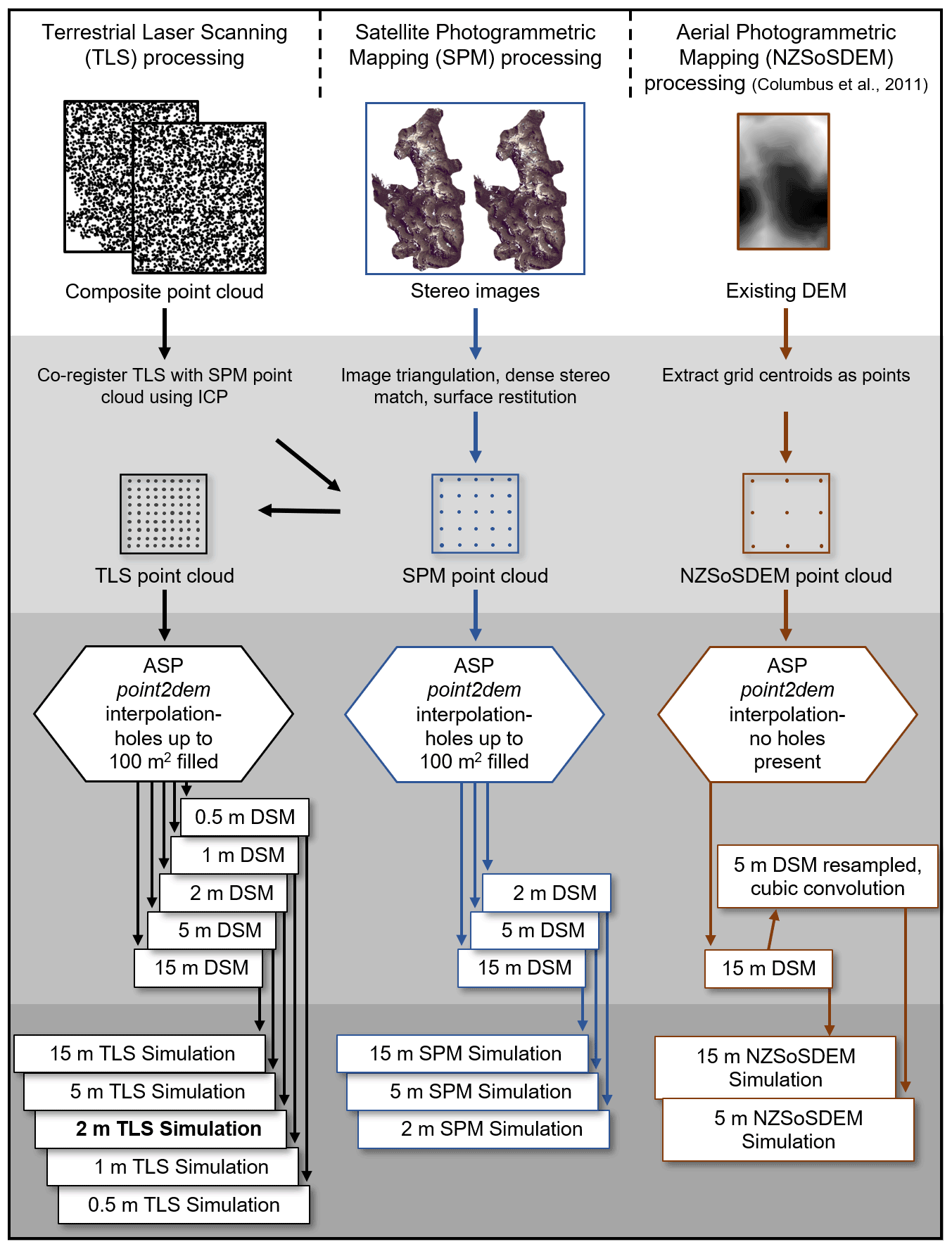
Figure 3Data processing workflow to generate the individual RAMMS simulations used to test the sensitivity of the dynamic model to topographic representation from the three input datasets: terrestrial laser scanning point cloud, Pléiades satellite bi-stereo images and the NZSoSDEM nationwide DEM for Aotearoa/New Zealand. The 2 m TLS reference simulation is noted in bold.
2.1 Digital surface model (DSM) generation
2.1.1 Satellite stereo imagery workflow
A cloud-free Pléiades-1B image stereo pair was acquired on 10 February 2020 at 10:37 NZST. The panchromatic and multispectral (red, green, blue, near-infrared) bands are provided with a spatial resolution of 0.5 and 2 m, respectively, with 12-bit radiometric resolution. The stereo pair had a base-over-height ratio () of 0.38. When processed with ground control points (GCPs), Airbus assesses Pléiades image horizontal accuracy with CE90 (circular error 90 %) as high as 0.35 m and vertical accuracy with LE90 (linear error 90 %) between 0.8 and 1.2 m depending on slope angle (Airbus, 2021), though higher vertical accuracy has been achieved (Eberhard et al., 2021; Stumpf et al., 2014). The imagery, captured as part of the Pléiades Glacier Observatory (PGO) program (ISIS/CNES), covered an area of 459 km2 of predominantly alpine terrain in Fiordland National Park. Acquisition was timed for late summer to minimize seasonal snow in the images.
The Pléiades image processing followed the workflow detailed in Eberhard et al. (2021) and included triangulation in ERDAS Imagine v2018 and surface restitution in NASA Ames Stereo Pipeline v2.7 (ASP, Beyer et al., 2018; Shean et al., 2016). We collected 10 GCPs over the imaged area alongside 29 tie points to triangulate the stereo pair with refined rational polynomial camera (RPC) modeling (Fig. 1). The GCPs were collected in 30 min fast-static mode for post-processing against permanent GNSS stations. Fixed solutions achieved centimeter-level precision, were converted to NZGD2000 and projected to NZ Transverse Mercator 2000 (EPSG:2193) using the rigorous deformation model provided by Toitū Te Whenua/Land Information New Zealand (LINZ). We assessed the quality of the triangulation using leave-one-out cross validation (LOOCV) (Eberhard et al., 2021; Sirguey and Cullen, 2014), which yielded a 0.45 m CE90 and 0.63 m LE90.
Dense stereo matching on the panchromatic bands at 0.5 m resolution was performed with a hybrid global-matching approach in ASP (Eberhard et al., 2021; Beyer et al., 2018; d'Angelo, 2016; Hirschmuller, 2008). We converted the resulting 0.5 m point cloud into a 2 m resolution DSM using the point2dem tool in ASP (Shean et al., 2016). The interpolation technique in point2dem calculates a Gaussian-weighted average of all points within a user-defined search radius set to 1.2× the cell size of the output DSM. DSMs at 5 and 15 m resolution were also directly generated from the 0.5 m point cloud to assess the sensitivity of avalanche simulations.
With point2dem we also generated a map of ray intersection errors which measures the minimal distance between rays derived from stereo matches. The map can be used to indicate the quality of the triangulated surface points, including the identification of areas of poor contrast where surface restitution is compromised (Eberhard et al., 2021). All elevation products use the NZTM2000 coordinate system with height above ellipsoid (HAE). For brevity, we will hereafter refer to the Pléiades-derived DSM products as SPM (satellite photogrammetric mapping). Finally, a point cloud was generated from the 2 m DSM in order to co-register the TLS data (see next section).
2.1.2 Terrestrial laser scanning workflow
A Riegl VZ-6000 terrestrial laser scanner was used to scan summer topography around Homer Tunnel on the Milford Road. The ultra-long-range scanner has a manufacturer-assessed accuracy of 0.015 m with an operational range exceeding 6 km. A composite point cloud of the Homer Tunnel area was created from 15 individual scans captured between 6 October 2019 and 27 February 2021 using Riegl's RiSCAN Pro v2.14 software. Multiple scans were needed to cover the entirety of the avalanche path and surrounding terrain as well as account for the steep topography and occluded terrain from the valley floor.
Scans of the alpine terrain were acquired between February and March to minimize seasonal snow. Areas of permanent snow in the upper release zone captured in more than one individual scan were manually cleaned to retain only the lowest points and avoid transient and seasonal snow, so the composite scan represented the minimum permanent snow level between 2019 and 2021. Manual cleaning of the composite point cloud was conducted in Riegl's RiSCAN Pro v2.14, where the reflectivity of the surface was leveraged to identify points associated with seasonal snow. An approximate vertical offset of 1 m between the points associated with the seasonal snow (removed) and the points associated with the permanent snow (retained) also helped with identifying points to be removed. Scans of the terrain adjacent to the road occurred at other times of year but only when free of snow (Table 1). The vegetation in the path is comprised of alpine grasses and shrubs (Fig. 2), which retain a similar structure throughout the year. A total of 323 checkpoints on objects visible in multiple scans with an average of 22 check points per individual scan were used to merge the individual scans into the composite point cloud. The mean deviation between checkpoints from scanning positions was 0.057 m. This point cloud (3.3 billion points) had varying point densities within the composite cloud so was thinned to an average point spacing of 0.15 m, or a total of 338 280 500 points.
Columbus et al. (2011)Table 1Description of the digital surface models (DSMs) used in RAMMS simulations and their derivations.
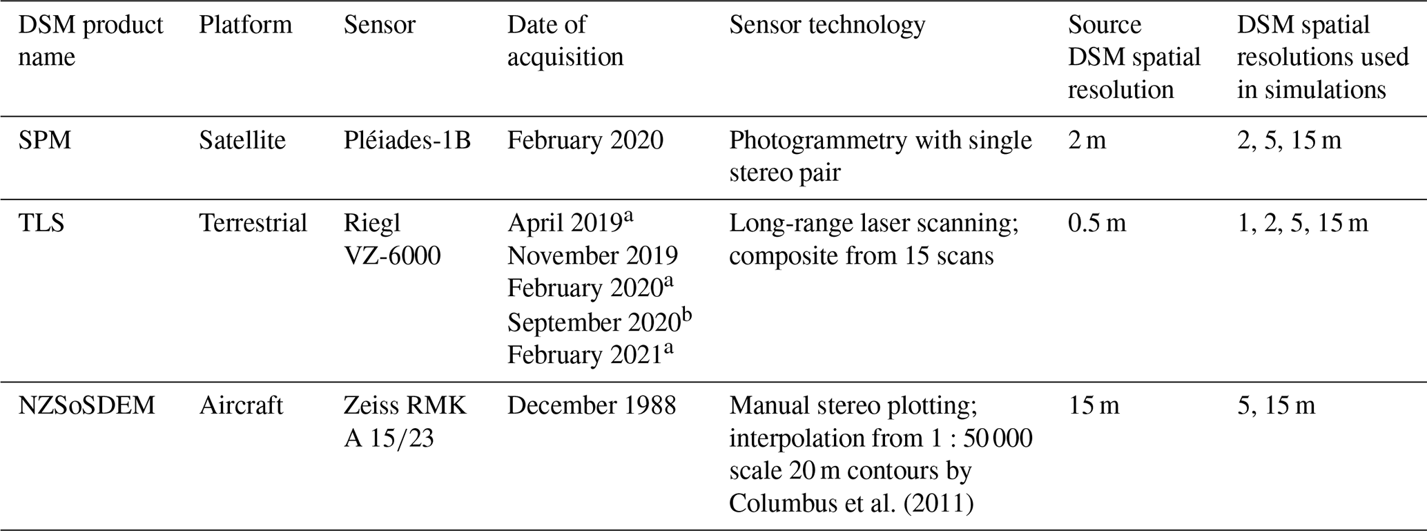
a Multiple scans conducted. b Scan used for avalanche documentation.
The composite TLS point cloud was generated in a relative coordinate system where the origin was located at the scanning position of the main scan approximately 50 m east of the Homer Tunnel entrance (see Fig. 1). The orientation was based on magnetic north and the internal laser plumb level. While the TLS point cloud was accurate in relative terms and could be used in hazard modeling without coordinate transformation, absolute georeferencing was required to compare simulations and was achieved by co-registration to the SPM point cloud. To minimize the influence of unreliable points in the SPM point cloud, the ray intersection error map was used to exclude points in areas of large intersection error generally corresponding to low image contrast (Sirguey, 2019). Specifically, a 12-cell rectangular median low pass filter was applied to the intersection error map. Points located in cells with an intersection error less than 2 m were sampled to retrieve a mean intersection error (0.13 m), which was used as a threshold for identifying pixels of low contrast. The segmented SPM points were visually checked for fit with shadows and other areas of low contrast (e.g., bright snow). While only segmented points were used for the co-registration of the TLS point cloud, the full DSMs used in the simulations included all points, to reflect the overall terrain representation in steep terrain with areas of variable contrast. Initial alignment of the TLS and segmented SPM point clouds was done manually in CloudCompare v2.10.2, and refined co-registration was achieved with the iterative closest point (ICP) algorithm (Rusinkiewicz and Levoy, 2001). The co-registered TLS point cloud was interpolated into a full-resolution 0.5 m DSM as well as 1, 2, 5 and 15 m DSM using the point2dem tool in ASP. The area of the 2 m DSM was 5.31 km2.
2.1.3 National elevation product workflow
We also incorporated the current national elevation product into the analysis. The last nationwide topographic mapping campaign produced a 1:50 000 scale topographic map with 20 m contours generated from analogue aerial photogrammetry in the 1980s. Images of the study site were captured in December 1988 and contours generated with stereo plotting. Contours were then interpolated into a 15 m DEM by Columbus et al. (2011) and released as the NZSoSDEM v1.0 product, which had a root mean square error (RMSE) of 7.1 m and mean absolute error (MAE) of 5.1 m compared with the national geodetic control network. For the purposes of the analysis, in addition to the full-resolution 15 m DEM, the NZSoSDEM was also downsampled to 5 m using cubic convolution for use in avalanche simulations. The DSM products used in the RAMMS simulations are summarized in Table 1.
2.1.4 Hole filling
High-resolution DEMs often contain holes, or data voids, which can cause issues with hazard modeling. Modeling applications often require DEMs to be conditioned to remove holes, pits, and other interpolation artifacts and errors (Reuter et al., 2007). Holes are primarily created when terrain is occluded from the sensor (in the case of TLS and SPM) or when there is low image contrast or clouds present in the image (in the case of SPM). Terrain occlusions are more acute with terrestrial sensors where the oblique angle to the terrain creates shadows behind topographic features and above-ground objects (Currier et al., 2019; Bühler et al., 2016). The steep relief in our study site also created terrain occlusions to the satellite sensor, generally limited to the terrain adjacent to the avalanche path. Combining point clouds from different scanning positions prior to interpolation mitigated the presence of holes in the TLS data, although some occluded terrain remained in the TLS composite scan.
Dynamic hazard modeling with RAMMS requires DEM continuity over the simulation domain. Although large voids were present outside the avalanche path due to terrain occlusions, our TLS and SPM point clouds only exhibited relatively small holes inside the path. Using the hole-filling option of the ASP point2dem tool with a threshold of 100 m2 was sufficient to fully fill all DEMs. The area of the path affected by hole filling was compared to a non-filled version of the 0.5 m TLS DEM. Within the RAMMS modeling domain, 3 % of the area was hole-filled for the 0.5 m DSM. This proportion reduced to zero or a marginal amount for DSMs interpolated at coarser resolution due to the larger search radius (e.g., 0.05 % for the 5 m TLS DSM). Figure 4 shows the full-resolution DSM for each surface (TLS, SPM, NZSoSDEM). Holes were present in the TLS and SPM surfaces, while no holes were present in the NZSoSDEM surface.

Figure 4Full-resolution DSMs for TLS surface at 0.5 m in panel (a), SPM surface at 2 m in panel (b) and NZSoSDEM surface at 15 m in panel (c). The 3D views focus on the lower cliff face and runout zone of McPherson path, corresponding with TLS 0.5 m surface in panel (d), SPM 2 m surface in panel (e) and NZSoSDEM 15 m surface in panel (f). The fracture line from the avalanche event is denoted with an orange line.
2.2 Avalanche event and simulation calibration
The McPherson avalanche was released with explosives dropped from a helicopter on 19 September 2020. The event was documented with videos from the ground and aboard the helicopter, satellite imagery, an infrasound array located down valley from the path (Watson et al., 2021), and three TLS scans of the release area and valley debris from the highway the following morning. The entire crown wall and most of the upper path was scanned (mean density of 19 points per square meter) with four smaller areas selected for increased point density (mean density of 468 points per square meter) to resolve the snowpack structure at the crown wall. Due to safety of the operator, only an oblique view of the debris was possible. An enhanced 3 m resolution four-band (red, green, blue, near-infrared) PlanetScope satellite image (Planet Team, 2020) acquired the following morning was used to manually digitize the debris in the valley. The terminus of the debris reached a large rock visible in both the imagery and the TLS.
The fracture depth (slope perpendicular) was calculated from the TLS scan. The fracture ranged from 1550 to 1780 m a.s.l. with a total length of 1346 m. A custom Python script was used to calculate crown wall height profiles along the fracture, which had a mean fracture depth of 1.53 m (range 0.003 to 2.95 m). The first visible slab failure occurred over 600 m from the explosive charge at the bottom of the first of three distinct release areas. They released 3, 5 and 6 s after the detonation. The release areas were manually digitized based on the fracture line and video evidence. Despite the large release area (total of 117 093 m2), this only accounted for approximately 20 % of the available terrain in the release zone.
An alpine weather station at 1700 m a.s.l. and located 600 m from the release area had a snow depth of 3 m and mean snow density of 400 kg m−3 at the time of the avalanche event. The freezing level dropped to 800 m a.s.l. for a period leading up to the most recent storm but then rose again to 1600 m a.s.l. where it stayed until the event. This meant there was a steep gradient of available snow for entrainment in the model from >3 m in the upper release area to no snow in the runout in the valley, which is common in Fiordland avalanche paths. The mean snow temperature in the top 1.5 m of snowpack at the weather station was −0.8 ∘C at the time of the avalanche, with a mean temperature of −1.3 ∘C in the remaining snowpack. For more detail on the weather and snow conditions in the month leading up to the event, see Watson et al. (2021).
The avalanche was simulated using the scientific (extended) version of RAMMS (Bartelt et al., 2016; Valero et al., 2016) and calibrated using the 2 m TLS DSM. The parameters for each model run are listed in Tables A1 and A2. The simulation used a two-layer mixed model simulating both the dense core (Buser and Bartelt, 2015) and the powder cloud (Bartelt et al., 2016). RAMMS implements a DEM as a function Z(X,Y) in a cartesian coordinate system where the independent variables x and y give the arc length along the surface and where the z coordinate is perpendicular to the slope (Christen et al., 2010b). RAMMS resamples the input DEM if the simulation grid size is smaller or larger than the input DEM resolution. Instead of resampling the DEM in RAMMS by altering the grid resolution of the simulation to be either finer or coarser than the input DEM resolution (Maggioni et al., 2013; Christen et al., 2010a), we ran each simulation with the associated grid size to the input DSM resolution. In other words, the TLS and SPM surfaces used in the RAMMS simulations were not resampled after the initial interpolation from the point cloud. This means that a greater number of elevation measurements are used to interpolate coarser DSMs. We did, however, resample the 15 m NZSoSDEM into a 5 m DSM using cubic convolution for the purposes of an additional comparison resolution.
RAMMS allows for more than one snow layer to correspond to different densities and temperatures with their own independent depths. We used two snow layers to better represent the structure of the snowpack based on the temperature profile of the snowpack at the nearby weather station and from the TLS scan of the remaining snow in the release after the event (Fig. 11). We calculated the mean snow temperature for both the upper 1.5 m and lower 1.5 m of the snowpack (the average fracture depth of 1.53 m) based on temperature values collected on 0.1 m intervals at the weather station. The mean temperature of the top layer was −0.8 ∘C, and the bottom layer had a mean temperature of −1.3 ∘C. RAMMS adjusts snow depth in the path based on the slope angle and curvature and with an elevation gradient to more realistically represent snow distribution on alpine terrain, as less snow tends to accumulate in very steep terrain (Sommer et al., 2015). The maximum snow depth was set to 3 m (two layers each with depth of 1.5 m) at 1700 m a.s.l., tapering to a depth of 0 m at 950 m a.s.l. For review of the extended RAMMS modules, see Buser and Bartelt (2015, 2009) on particle movement; Fischer et al. (2012) on curvature effects; Bartelt et al. (2015) on cohesion within the core; Valero et al. (2016, 2015) on warm, wet avalanches; and Ivanova et al. (2022), Bartelt et al. (2016) and Dreier et al. (2016) on the powder cloud. While the snow temperature and density values recorded in the snowpack at the time of the avalanche are usually associated with wet avalanches, the terrain in the McPherson path produced a powder cloud nonetheless.
Based on video evidence of the avalanche and satellite imagery showing the debris pattern in the valley, as well as the TLS scans, the simulation matched the documentation for the powder cloud behavior (frontal velocity and areal extent) and final debris pattern. The simulation was then re-run using the TLS 0.5, 1, 5, and 15 m DSMs; the SPM 2, 5, and 15 m DSMs; and the NZSoSDEM 5 and 15 m DSMs with all snow parameters remaining constant. In other words, the only difference between simulations was the elevation model source and/or resolution. The 0.5 m TLS is not included in the results because the processing requirements for the size of the avalanche made it impracticable. In addition to testing the different DSM sources and resolutions, we also ran simulations with a deeper snowpack to mimic a smoother winter surface where small terrain features would be covered by snow. The lower depth value was increased from 1.5 to 3 m (total depth of 4.5 m) at 1700 m a.s.l. The lower layer temperature remained at −1.3 ∘C. All other parameters were held constant and both the TLS and SPM 2 m simulations were re-run with the additional snow available for entrainment in the path.
2.3 Differences in topographic representation
To compare the differences in topographic representation between the surface models, DEMs of difference (DoDs) were calculated between the DSM sources. Typically used for detection of landscape change (Berthier et al., 2014; Lague et al., 2013; Wheaton et al., 2009), here the DoD was used to identify areas of the avalanche path with different elevation values between DSMs from a range of possible drivers. These include acquisition timing (e.g., presence of seasonal snow), angle to the sensor and spatial resolution, artifacts in the interpolation of holes in the DSM, or uncertainty in the stereo matching for the photogrammetry-derived DSM, which all could affect how topographic features important for hazard modeling, like gullies or cliff faces, are represented in the surface model. The DoDs, expressed as , where Z1 and Z2, correspond to the DSM with the same resolution but different source, for example TLS2 m−SPM2 m. The results of the DoDs focus on terrain differences between the TLS and SPM DSMs which were co-registered and where fine-scale terrain feature differences will be most pronounced compared with the NZSoSDEM, owing to their higher spatial resolutions. The results of the DoD and implications for the avalanche simulation are provided in Sect. 3.5.
The McPherson avalanche released in three distinct areas in quick succession. Snow from the first and smallest release area was the first to flow over the lower cliff band; however, the flow from the second and third release areas generated the greatest core and powder cloud velocities. It went over the upper cliff with average slope angle of 64∘, crossed a shelf with an average slope angle of 13∘, and then plunged over the lower cliff with an average slope angle of 76∘, ejecting the core into the air (see Fig. 5). Despite the warm snow temperature, a large powder cloud was generated. The avalanche reached the valley floor approximately 39 s after the explosive charge detonated. The core traveled over 500 m down the valley before terminating at a large rock visible in both the TLS point cloud and PlanetScope satellite image. The average slope angle between the lower cliff and the terminus rock was 13∘. The avalanche had a total length of approximately 1400 m from the highest reach of the fracture line to the toe of the debris in the runout. The powder cloud reached maximum velocity in the upper portion of the valley but was visible as it lightly drifted past the Homer Tunnel entrance, 500 m further than the core.

Figure 5Images of McPherson avalanche event as the core runs over the lower cliff (left panel) and powder cloud accelerates into the valley (right panel) taken from video documentation of event. Courtesy of Downer Ltd. Milford Road Alliance.
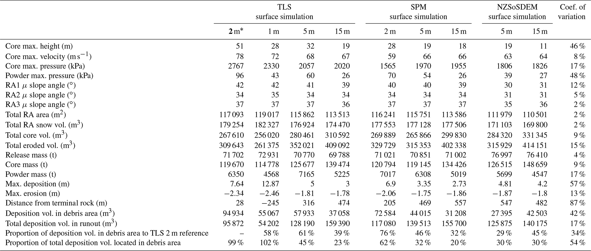
Table 2Results of RAMMS simulations for DSM resolution by elevation source: terrestrial laser scanning (TLS), satellite photogrammetric mapping (SPM), and analogue aerial photogrammetry (NZSoSDEM) and the coefficient of variation for all simulations. All simulation parameters held constant after calibration based on TLS 2 m DSM (bolded). Release area (RA) has been abbreviated.
* Reference simulation calibrated against avalanche event documentation.
3.1 Calibration simulation
The TLS 2 m calibration simulation matched the core flow and powder cloud behavior provided by the documentation. Simulation results are summarized in Table 2. The maximum estimated deposition depth was 7.6 m, and the maximum estimated erosion depth in the track was −2.3 m. The total volume calculated inside the deposition area identified by the TLS and PlanetScope image was 94 934 m3, accounting for 99 % of the total simulated deposition below the lower cliff. The simulated avalanche had a release volume of 179 254 m3 (similar to the 1968 Swiss In den Arelen avalanche; Christen et al., 2010a) and release mass of 71 702 t. The total core mass was estimated at 119 670 t. It was a large avalanche despite the relatively short total length. By the Canadian avalanche size classification used internationally (Moner et al., 2013; McClung and Shaerer, 1980), the simulation suggested the avalanche was a size 5 (defined as an avalanche having a total length >3 km and/or volume >100 000 m3). The avalanche core was estimated to have a maximum flow height of 51 m and maximum pressure of 1383 kPa. The powder cloud was estimated to have a maximum height of 330 m and pressure of 96 kPa (Table 2). Powder pressures exceeding 5 kPa covered over 21.8 ha of the path and adjacent valley walls and were greatest at the bottom of the lower cliff.
The maximum core velocity, which is calculated as the mean of the maximum velocity profile values for a given cell, was 78 m s−1 or 280 km h−1. Figure 6 shows the estimated maximum core velocity and maximum powder pressure. Core velocities were greatest as the core flowed over the top of the lower cliff, while the powder cloud velocities were greatest as the core splashed over terrain at the bottom of the cliffs, rapidly pushing air in front of the core and accelerating away from the cliff. The simulated avalanche hit the valley bottom 41 s after the explosive charge (2 s slower than video evidence), so the velocity estimates are conservative. The plunging nature of the avalanche over the lower cliff adds complexity to the modeling. The sharp transition in the upper path between the steep terrain into the lower angle shelf accelerated the core such that it went airborne over the second, steeper cliff. The complex relationship between slope angle and the core velocity can be seen with the plot in Fig. 6 that shows the influence of the slope transitions in the upper and lower path. The greatest powder pressures were estimated when the core splashed into the valley.
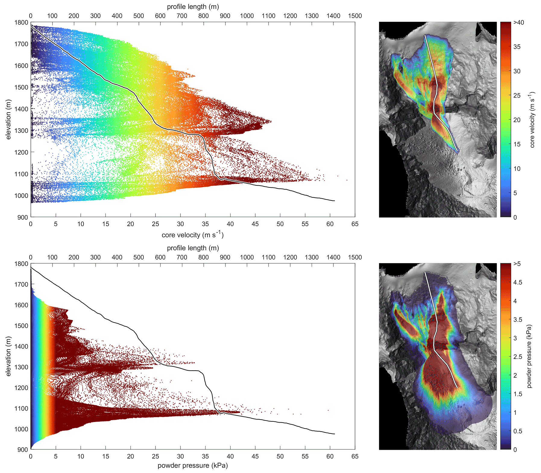
Figure 6Results of TLS 2 m calibration simulation showing maximum estimated core velocity (top panels) and powder cloud pressure (bottom panels). The core velocity saturates red at 40 m s−1, while the powder pressure saturates red at 5 kPa. The track profile is shown in the plots for context of the location of the cliff, shelf and runout.
3.2 Simulation differences by DSM resolution
This section outlines how using the same DSM source (TLS-derived) but changing the resolution (1, 5, 15 m) affected the simulated avalanche behavior. The surface difference (estimate of erosion and deposition) for each simulation is shown in Fig. 7 grouped by DSM resolution. The general pattern is that coarser-resolution simulations (5 and 15 m) resulted in the avalanche core traveling too far down the valley and thinning out in the deposition area, the result of the DSM interpolation smoothing microtopography. With larger cell sizes (coarser DSMs) the release areas are smoother, resulting in lower initial snow volumes. However, increasing the cell size increased the volume of snow entrained in the core and the total eroded snow volume. Likewise, the release mass was smaller with coarser DSMs, but the total core mass was larger (2 m was 119 670 t; 5 m was 125 677 t; 15 m was 139 474 t). The mass of the core that is converted to the powder cloud had no linear relationship with DSM resolution. However, the maximum estimated powder cloud pressure (kPa) did decrease with increasingly coarse DSM resolution. The exception was the 1 m DSM, which generated a smaller powder cloud since much less mass was ejected over the lower cliff.
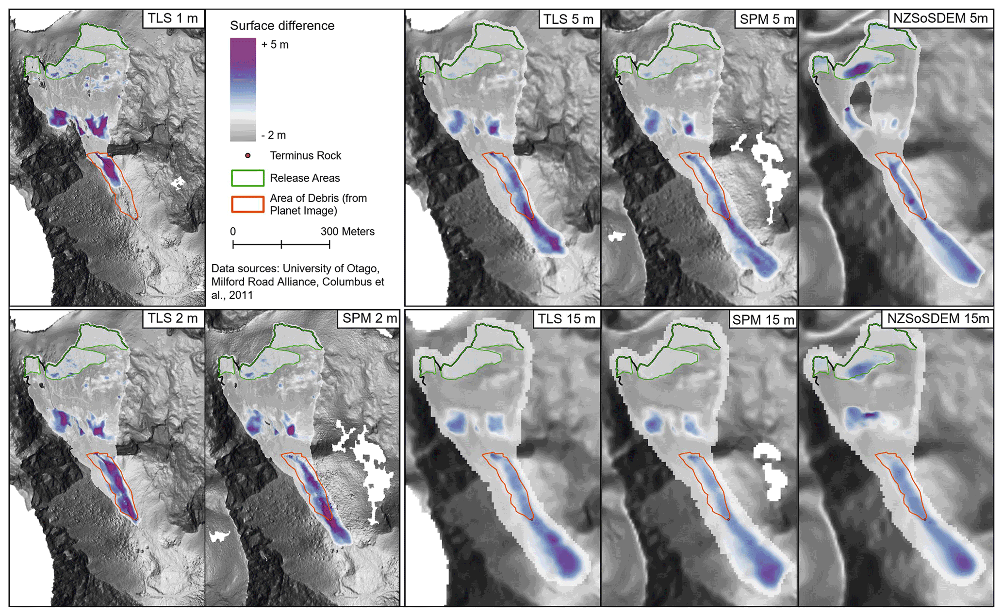
Figure 7Composite of simulation outputs for TLS, SPM and NZSoSDEM DSMs showing surface difference areas of estimated erosion and deposition. Outputs are grouped by resolution. The fracture line, release areas and debris area are shown in each map. The event was calibrated on the TLS 2 m DSM.
We found that the most objective and useful results for comparing simulations are the runout distance, calculated as the distance between the debris toe and the terminus rock where the real avalanche stopped, as well as the deposition volume located in the documented debris area, relative to the 2 m TLS reference simulation. The highest-resolution 1 m TLS simulation showed the avalanche stopping short of the real avalanche (245 m before the terminus rock), with much of the initial entrained snow getting stuck on the shelf above the lower cliff. The 1 m simulation resulted in the deepest estimated deposition (12.87 m) as snow piled up on the shelf. While the snow volume in the release areas was greater than any other simulation, owing to the higher surface roughness, less snow was eroded, and the core mass was lower than with the 2, 5 and 15 m simulations. The powder cloud was also smaller with less mass converting from the core to powder cloud and dissipating midway down the valley.
The 5 m TLS simulation resulted in the core traveling too far down the valley with the toe of debris 316 m beyond the terminus rock. The maximum estimated debris depth was 5 m, and the maximum estimated erosion was −1.81 m. While the volume of snow in the release areas was lower than in the 2 m simulation, the 5 m simulation had a larger core, eroding more snow. The total volume of snow in the documented debris area (57 933 m3) was 39 % less than in the reference 2 m simulation as the core maintained momentum further down the valley. Only 45 % of the total debris volume was located in the documented area. The powder cloud covered a larger area compared with the 2 m reference simulation with powder reaching Homer Tunnel at 20 m s−1 and extending well past the highway. At the same time, the powder cloud had a lower estimated maximum pressure compared with the 2 m reference simulation.
The 15 m TLS simulation also resulted in the core traveling too far down the valley with the toe of the debris 474 m from the terminus rock. The maximum debris height was only 3 m and erosion −1.78 m. The 15 m simulation had the largest total eroded volume (409 092 m3) and core mass (139 474 t). The total debris volume in the documented area was 37 058 m3, 61 % less than the 2 m reference simulation, resulting in only 23 % of the total debris volume located inside the documented area as most debris was spread further down valley. The powder cloud covered a larger area than the 2 or 5 m simulations reaching Homer Tunnel with velocities of 30 m s−1 and extending well past the highway. The powder cloud had the lowest maximum pressure compared with the other TLS simulations. It also maintained a more uniform shape around the core in the valley, with little lateral spreading to edges seen in the 1, 2 and 5 m simulations. Figure 8 compares the deposition pattern differences between TLS 1, 2, 5 and 15 m simulations as a profile from the lower cliff face to the furthest reach of simulated debris.
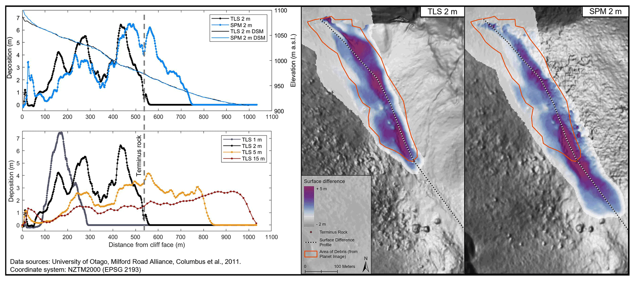
Figure 8Profile of simulated debris from lower cliff face through runout zone between TLS and SPM 2 m simulations (top left panel), including the 2 m TLS and SPM elevation profile for reference, and between TLS 1, 2, 5 and 15 m simulations (lower left panel). Examples of simulated debris patterns for TLS and SPM 2 m simulations (right side panel) show how well debris pattern matches documentation (orange polygon).
3.3 Simulation differences by DSM source
This section compares simulation results between DSM source (TLS, SPM and NZSoSDEM). The 2 m TLS and 2 m SPM simulations were similar in a number of ways (see Fig. 7 and Table 2). Overall, the 2 m SPM DSM best matched the pattern of surface difference of the 2 m TLS calibration simulation; however, clear differences remain. The debris in the 2 m SPM simulation overshot the terminus rock by 205 m and left less debris on shelf between cliffs. The 2 m SPM simulation had a maximum deposition depth of 6.9 m and erosion of −2.06 m. Figure 8 compares the surface difference profiles between the 2 m TLS and SPM simulations and shows the SPM core traveling further down valley but with a similar deposition pattern.
While the release volumes and total core volumes were similar between the 2 m simulations, the 2 m SPM simulation eroded a greater volume of snow (329 729 m3 compared with 309 643 m3) and converted more mass to powder (7017 t compared with 6350 t). The 2 m SPM simulation deposited 24 % less volume inside the documented release area compared with the 2 m TLS calibration simulation. Only 62 % of the total deposition volume in the valley was located inside the documented debris area. The core and powder velocities were slower, and the maximum core height and maximum powder pressures were lower than the 2 m TLS simulation.
There were 5 m simulations run on the TLS, SPM and NZSoSDEM surfaces, which exhibited substantial differences (Fig. 7c). The NZSoSDEM simulation had the longest run beyond the terminus rock (547 m) compared with the TLS and SPM 5 m simulations (316 and 469 m respectively). It had the least lateral spread and was concentrated in the middle of the valley, while the TLS and SPM better captured the actual flow pattern. The total volume of snow in the release areas were more similar at 5 m compared with 2 m as small topographic features begin to be smoothed, though the NZSoSDEM volume was lower (171 103 m3) compared with the TLS (176 924 m3) and SPM (177 128 m3) simulations. The 5 m TLS simulation eroded the most snow (352 021 m3) compared with the SPM (315 353 m3) and NZSoSDEM (315 929 m3). While none of the 5 m simulations matched the final debris pattern in the valley, the TLS had the greatest proportion of total debris volume (45 %) located in the debris area. The SPM (32 %) and NZSoSDEM (30 %) had debris stop further down the valley. Similarities between the 5 m simulations include the core and powder velocities and powder pressures.
The 15 m simulations, also run on the TLS, SPM and NZSoSDEM surfaces, produced the most similar results (Fig. 7). All three simulations showed the core traveling too far down the valley with the bulk of the debris stopping well beyond the terminus rock. The maximum deposition and erosion was smaller owing to the spreading of the debris over a larger area compared with higher-resolution simulations. Despite further smoothing of small topographic features with increased DSM resolution, differences remain in how the avalanches entrain snow into the core (total core volume for TLS: 310 952 m3; SPM: 299 830 m3; NZSoSDEM: 331 345 m3). The total eroded volume followed the same pattern, with the 15 m NZSoSDEM generating the largest core flow but converting the least mass into the powder cloud. None of the three simulations characterized the final debris pattern in the valley, with only 23 % of the 15 m TLS debris volume located in the debris area and only 20 % and 30 % for the SPM and NZSoSDEM respectively. While the maximum estimated core height was significantly greater between the TLS and SPM 2 and 5 m simulations, the core heights were similar in the 15 m simulations. The core and powder velocities and powder pressure were similar in all three surfaces. See Table 2 for summary of simulation outputs for each DSM and resolution.
3.4 Additional snow available for entrainment
We increased the depth of snow cover in the path, while keeping the average release depth the same, to mimic the avalanche flowing on a more-snow-filled surface. Increasing the overall snowpack depth kept the release volume the same in the SPM simulation but actually decreased it marginally in the TLS (179 254 to 178 667 m3) simulation showing the effect of resolving fine-scale terrain features. We found a similar pattern of difference between the TLS and SPM 2 m DSMs. Compared with the TLS simulation, the SPM had a lower maximum core flow height (28 m vs. 43 m) and lower core velocity (58 m s−1 vs. 71 m s−1). It nonetheless produced a larger avalanche by entraining more snow in the path (total core volume was 337 949 m3 vs. 323 204 m3 and total eroded volume was 481 545 m3 vs. 439 686 m3) and had a longer runout, traveling 201 m past the terminus rock, compared with 146 m for the TLS simulation. Interestingly, the runout distance was nominally the same for the SPM simulation run with and without the deeper snowpack, where the TLS simulation run with the deeper snowpack ran over 100 m further down the valley. In other words increasing the available snow in the path led to increased entrainment and total core volume in both simulations. While the TLS simulation ran further down the valley, the SPM simulation did not, which suggests that decreasing the surface roughness of the sliding surface affected the TLS simulation more.

Figure 9DEM of difference (DoD) map showing topographic differences between TLS 2 m and SPM 2 m DSMs. The areas of poor contrast in SPM imagery are shown with hash polygon. The 3D panel focuses on differences in topography where snow melt occurred between data acquisitions and on the extent to which gully features are resolved in the DSMs.
3.5 Topographic differences between DSMs
The DoD between the TLS-derived surface and the SPM-derived surface highlights important differences in the representation of terrain in the avalanche path. Since the denser TLS point cloud was registered to the SPM point cloud, overall the two surfaces are well aligned (Fig. 9). The mean cell-to-cell difference for the entire 5.31 km2 TLS2 m−SPM2 m study domain was −0.13 m (RMSE = 4.25 m). The greatest differences are in areas of poor contrast in the SPM surface and in the cliff faces. For example, approximately 53 % of the documented debris area in the valley was in shadow when the SPM satellite imagery was acquired. This area had a mean cell-to-cell difference of −0.7 m (RMSE = 4.17 m) compared with −0.1 m (RMSE = 0.64 m) in the remaining shadow-free portion of the debris area. The DoD results from steep terrain should be viewed with caution as large errors can be created with cell-to-cell misalignment for the same terrain in two surfaces (Lague et al., 2013). Resolving sharp cliff edges in two DEMs, for example, can create large elevation differences.
Nonetheless, subtle but consequential differences in the shape of the surface in gully features in the track and the delineation of cliff edges led to notable differences between the TLS and SPM surfaces. This is especially evident in the upper portion of the path where the orientation of gullies created poor view angles to the satellite when imaged, and the true shape of the gully features was not captured in the SPM DSM. Gulley features on the order of 5–10 m deep and 10–20 m across were found to divert the core flow of the avalanche in the track. The presence of seasonal snow on the bench between cliffs in the path also created marked differences in surface elevation and roughness between DSMs.
After the McPherson avalanche was calibrated in RAMMS, the DSM data source and spatial resolution test revealed how differences in topographic modeling affected simulated avalanche behavior. Like Bühler et al. (2011), who compared DEM sources and spatial resolution in RAMMS simulations, we found that increasingly coarse DSMs create longer core runouts. We also found powder cloud pressures, and velocities varied considerably between finer- and coarser-resolution DSMs. At the same time, subtle differences in terrain representation, based on the sensor technology and orientation to the terrain, also affected the simulated avalanche behavior between high-resolution 2 m DSMs generated from terrestrial laser scanning (TLS) and satellite photogrammetric mapping (SPM). In this section we will put some of the results in larger context, especially with regards to surface roughness and channelized terrain features. We will then discuss the implications for mass movement modeling posed by our study and make suggestions for hazard researchers and practitioners considering which elevation product to use in their modeling.
Testing differences in DSMs for snow avalanche modeling is a challenge because of the differences in the representation of above-ground features such as trees and bushes and their effect on measures of surface roughness. To avoid the influence of these features in the surface roughness, we simulated a snow avalanche that was flowing in a path lacking these above-ground features.

Figure 10Composite map comparing slope angle and surface roughness for the TLS-derived 2 m DSM and satellite-derived (SPM) 2 m DSMs. Panel (a) shows TLS 2 m slope angle, panel (b) shows SPM 2 m slope angle, and panel (c) is the SPM ortho-image showing fracture line and debris area. Panel (d) is TLS 2 m surface roughness, panel (e) is the SPM 2 m surface roughness, and panel (f) is the difference in surface roughness between TLS and SPM 2 m DSMs, which also shows the digitized release areas used in the simulation.
4.1 Differences in surface roughness
Figure 10 compares the roughness between the 2 m TLS and SPM surfaces. Roughness was calculated as the vector ruggedness measure (VRM) (Sappington et al., 2007), which has performed well at characterizing roughness for avalanche modeling (Bühler et al., 2022; Brožová et al., 2021; Bühler et al., 2018). We used a moving window area of 64 m2 (4×4 cell neighborhood) to assess differences in roughness between the 2 m DSMs. We also differenced the roughness maps to identify areas of diverging roughness. Overall the TLS-derived DSM has higher surface roughness throughout the path – the result of a higher point density in the point cloud before interpolation. Important differences are nonetheless still evident. The TLS is rougher in gulley, or channel, features in the bedrock located throughout the track. These channels are not fully resolved in the SPM-derived DSM, resulting in lower localized relief and thus lower surface roughness. Resolving these fine-scale terrain features in the TLS-derived surface meant more of the simulated avalanche core flowed through the channels in the upper track instead of spreading out, likely increasing overall entrainment. If the Pléiades satellite had a different orientation to the ground when the images were captured, or acquired as a tri-stereo image triplet, these features may have been more fully resolved.
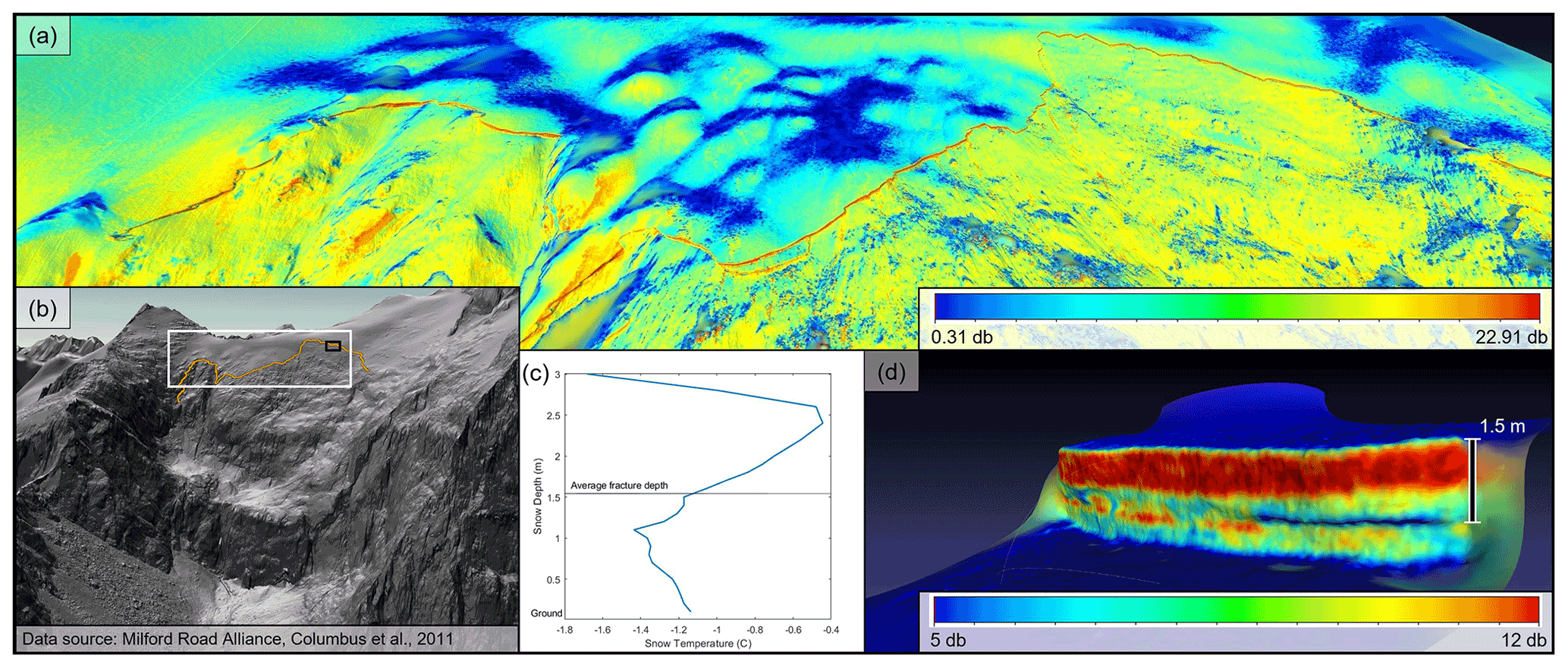
Figure 11Composite showing amplitude of lidar return from scan of the release area the morning after the avalanche event in panel (a). Panel (b) is a hillshade of the avalanche path from the 0.5 m full-resolution TLS-derived DSM, which also depicts the location of panel (a) in white and panel (d) in black. Panel (c) shows the temperature profile of the snowpack at the closest weather station at 1700 m a.s.l. and depicts the average fracture depth used for the RAMMS simulations, based on the TLS data. Panel (d) shows a higher-resolution scan of the face of the crown wall from the morning after the avalanche, also visualizing the amplitude. Note the different scale bar ranges. The snow depth value in panel (d) is indicative of the average fracture depth for the avalanche.
Differences in roughness are also evident in the runout, where part of the valley was in shadow at the time of the Pléiades image acquisition. The lower signal-to-noise ratio in the shadow promotes variability in stereo matching and increases noise in the DSM (Eberhard et al., 2021), which in turn increases the apparent roughness. Since this was in the runout where the avalanche core had reached near-maximum velocity, the effect on the simulation results was reduced. However, the presence of shadow or other areas of low image contrast (e.g., saturated snow) should be considered when using photogrammetry-derived DSMs and can be mitigated depending on terrain orientation, region and date of imaging.
Differences in roughness in the release zones are also apparent, and the lower friction with the SPM surface may have increased both initial core velocity and entrainment. Differences in slope angle (Fig. 10) also show the smoothing of cliff edges in the SPM surface due to shadowing, large parallax and challenging geometry. Less crisply defined cliffs may have created conditions for the core to slide rather than eject over the cliff edge, potentially maintaining momentum for the core to travel further in the runout.
Figure 11 shows a scan of the release area the day after the event. By visualizing the amplitude of the returning light energy to the sensor, we can highlight differences in material – snow surface that did not avalanche, snow on the exposed surface after the avalanche and rock. The fracture line corresponded with the edge of the permanent snow seen in both the TLS and SPM surfaces. While the initial sliding of the avalanche slab may have been on a smoother snow surface than is represented by the DSMs, the avalanche removed most of the snowpack, followed by the avalanche tail depositing a shallow amount of snow on the bedrock in the release area. A DSM with higher roughness created a more realistic surface for this event after the initial slab started sliding. Due to resolution limits, the smoother SPM DSM did not capture the fine-scale rough bedrock features captured in the TLS data after the avalanche. This was again evident when simulating the event with additional snow in the path to mimic a smoother winter surface. While the deeper snowpack resulted in more entrainment in the track, there was marginally more deposition in the release areas compared with the shallower (actual) snowpack depth. The lack of erosion suggests the rough source surface still has an influence in the release dynamics. In the case of the McPherson avalanche, using a DSM – and one that better resolves the true roughness of the terrain – improved the modeling. A newer generation of satellite sensors such as Pléiades Neo, which nearly halves the spatial resolution from Pléiades, will improve the terrain representation in rough alpine terrain lacking trees and shrubs.
Differences in how the shelf between cliffs in the track was resolved in the TLS and SPM 2 m DSMs also contributed to diverging core flow characteristics. More snow in the TLS simulation stopped on the shelf, which may partially explain the shorter (and more accurate) runout distance. The core reached the shelf first in the SPM simulation, which better matched the timing from video evidence and again illustrates that the smoother sliding surface in the release zone led to higher initial core velocities. Figure 12 shows the core as it flowed over the shelf at two time steps in the simulation (t=35 and t=40 s) for both the SPM and TLS 2 m DSMs. The smoother SPM surface meant the core traveled more directly down the track instead of moving through the channels present in the terrain. Fine-scale channeling and protrusions from seasonal snow diverted the core flow in both simulations but to a greater extent in the TLS simulation. With increasingly coarse simulations, these features and become less influential. For example, in the 5 m TLS simulation some channelized flow is evident, but with the 15 m TLS simulation the core flows straight over the shelf in a more homogeneous pattern. Slight differences in the distribution of seasonal snow on the bench at the time of the data acquisition for both the TLS and SPM surfaces are also evident.
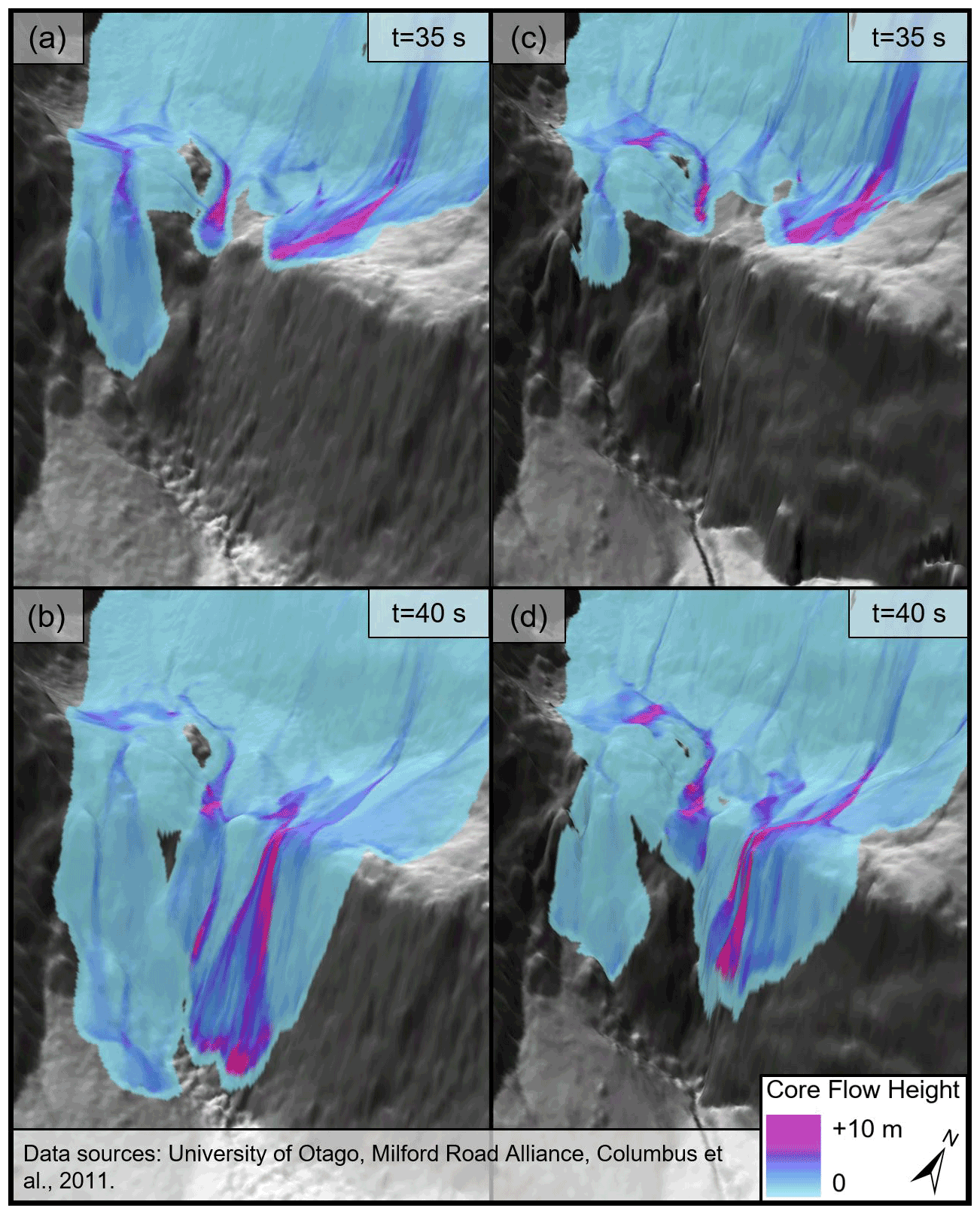
Figure 12Composite map showing the estimated core flow height at two time steps for both the TLS and SPM 2 m DSMs. Panel (a) shows the SPM DSM and panel (c) shows the TLS DSM both at t=35 s in the simulation. Panel (b) shows the SPM DSM and panel (d) the TLS DSM at t=40 s in the simulation. For spatial context, the cliff face shown in the composite is approximately 200 m in height.
4.2 Effects of elevation source and spatial resolution on mass movement modeling
These differences have implications for the ways in which model outputs are used (e.g., infrastructure design) but can also help clarify how certain topographic features may alter predicted avalanche behavior, which can be considered by the modeler when deciding on which elevation source and resolution to use. This study focused on an avalanche path without trees, where a DSM is a better representation of the actual terrain because of the rough nature of exposed bedrock as the sliding surface throughout the track and runout zone. For terrain with high surface roughness, removing the first return in a lidar point cloud to create a DTM may create an over-smoothed surface for use in modeling. This may be appropriate in the release zone but not elsewhere in the path (Brožová et al., 2021), especially for smaller avalanches that may not break to the ground. The terrain and nature of this avalanche were such that the surface that better captured the true roughness improved the dynamics in the release area as well. Our case may not be common to many sub-alpine modeling applications, especially where the study site involves trees and shrubs. However, it shows the value of using a DSM for many alpine cases. Fundamental differences in the way terrain is represented can be traced back to the way it is captured. Photogrammetry – irrespective of platform – typically relies on two or more view angles from the sensor to the imaged surface, with a tension between the desire for high ratio for matching accuracy and low incidence angles to avoid obstructions. Obstructions between an imaged area and the sensor by terrain in one image of a stereo pair will create a data void or hole in the DSM. Likewise, areas of cloud and areas of poor local contrast, such as deep shadow or homogeneous snow, confound stereo matching and either increase noise or create holes in the surface. These holes can be mitigated by increasing the number of images used in stereo restitution to achieve additional view angles (e.g., tri-stereo instead of stereo, multiview stereo and structure-from-motion products) and/or using improved radiometric resolution suitable to the targets to be imaged. The presence of clouds cannot be mitigated and depending on the region may impact success of tasking; however, increased temporal resolution of imaging can increase the probability of cloud-free images.
Interpolators can be used to fill holes, but the size of the hole to be filled should be a considered carefully and the relevance assessed based on predominant aspects and where holes are located in the modeling domain. For example, in this study most of the large holes were located in terrain where the simulation was unlikely to encounter them on steep walls adjacent to the path. These holes were not filled based on our threshold of 100 m2. Working with lower-resolution DEMs will decrease the proportion of the domain covered by holes as smaller holes will be filled with standard interpolation. Thought should also be given to how the interpolation of holes is likely to create an unrealistically smooth representation of terrain, which, as discussed, has implications for how a simulated mass movement flows over the terrain.
Lidar can mitigate the presence of holes in the DEM as areas of poor contrast will not meaningfully impact the measurements. However, holes from obstructed view of the terrain remain. TLS-derived DEMs are more likely to have holes given the oblique scan angle to the terrain but can be mitigated with multiple scans used to build a composite. Manual cleaning of the point cloud is likely needed to avoid artifacts. Local sinks and spikes can create spurious simulation results. This is particularly important in terrain with extreme roughness (jagged cliffs, crevasses, overhangs) where points can be misappropriated to an output cell in the interpolation. The difference between a summer and winter surface is especially pronounced in glaciated terrain where crevasses will be filled with snow in winter (making the surface smoother) and free of snow in summer, creating deep slope-perpendicular channels in a DEM. Filtering may be necessary to fill these features for use in avalanche modeling.
The wide range of terrain considerations means there should not be a universally recommended simulation resolution for hazard models (Bühler et al., 2011; Claessens et al., 2005). The rate of landscape change in many regions means the elevation data might not reflect the true terrain if captured some time before the modeling. At the same time, previous avalanching may create a different surface for the avalanche to run on than what is represented by the DEM. Generally, these factors become less important with coarser DEMs. We found that the 15 m DSMs produced the most similar simulations since the influence of fine-scale terrain features is dampened or removed. However, a loss of permanent snow in the upper portion of the path since the 1988 aerial imagery used to generate the NZSoSDEM created steeper, rougher terrain evident in the TLS and SPM 15 m DSMs, altering the core flow characteristics in the upper portion of the track. Downsampling the 15 m NZSoSDEM to 5 m also created artifacts in the simulation with a significant deposition of snow in the lower part of one release area. The age of the DEM, especially in alpine regions, should be a consideration for whether the DEM is appropriate to use for modeling.
4.3 Implications of study results
While the combination of terrain (steep, rough, rock faces, treeless) and snowpack (warm, deep with a steep elevation gradient) in the study site may limit the direct transferability of our findings to other sites with different topographic and climatic settings, results from this analysis can be of operational use to hazard modelers and practitioners nonetheless. We urge caution when using coarser DEMs (>5 m) for RAMMS modeling in complex terrain where the influence of microtopographic features such as gulleys or channels will affect the simulated flow of the avalanche and any operational decision-making based on the modeling results. Just as experts calibrate dynamic hazard models for the specific snowpack of a simulated avalanche (i.e., density, temperature), similar topographic calibration should be undertaken as well. This may entail multiple model runs adjusting only the resolution of the DEM to compare against event documentation or testing both a DSM and DTM in calibration runs, if the choice exists. We found the total runout length and the proportion of the estimated volume located in the documented debris area to be the most useful model results for distinguishing model runs from one another and linking model results to the underlying terrain representation in the DSM.
Overall the coarser DSMs in our study poorly captured the characteristics of the McPherson avalanche, with implications for design specifications for infrastructure or operational decision-making. For example, estimated impact pressures varied considerably between simulations and were largest in the highest-resolution DSMs where channelized terrain features were resolved, compared with the coarser DSMs where the core spreads out more. The most accurate estimates for roading infrastructure design would need to account for these subtle terrain features. Overall, we found that the use of a coarse DEM for avalanche modeling in steep, rough alpine terrain is not appropriate. However, this is often the only DEM product available to modelers in many alpine regions. Upsampling the coarse DEM to a higher resolution will not improve the representation of terrain or the model. At the same time, the use of a very-high-resolution (<2 m) DEM not only drastically increases the model processing time but also does not improve the results. We found the 1 m TLS-derived DSM simulation had too much friction and the simulated avalanche failed to replicate the behavior of the documented avalanche. This is most important in the upper path where the finely resolved features were too rough for the avalanche to gain momentum appropriately.
As the number of high-resolution DEMs in alpine regions increases, absolute accuracy of each DEM will become more important. Currently, the patchwork of elevation products in many areas means it can be challenging to assess the accuracy of a project-based DEM against a reference DEM. This is not an issue with many modeling applications where a DEM with high relative accuracy is sufficient. However, with many disparate DEMs produced through time, absolute accuracy becomes important to quantify landscape change, detect artifacts in the DEM, and tie in with other contextual data, related to, for example, infrastructure or land use.
Aerial lidar, not available for our study, would allow for additional sensitivity testing given the orientation difference to the sensor and the expected completeness in the output DEM. Nonetheless, some of the jagged and overhanging cliff faces are better captured from the ground. An advantage of the TLS is also rapid deployment after an event to refine model parameters and provide snowpack distribution information for forecasters (Prokop et al., 2015; Thibert et al., 2015; Deems et al., 2015; Maggioni et al., 2013; Prokop, 2008; Sailer et al., 2008) as an alternative to more costly aerial lidar (e.g., Sovilla et al., 2010). In our case the scan of the release zone from the following morning provided important information on the characteristics of the avalanche. Remote sensing techniques were the only viable option to estimate the release depth and identify where in the snowpack the weak layer was located. Figure 11 shows how remotely measuring the crown wall and correlating the weather station data on snow temperature and density was used for precise model parameterization. The slab that released is discernible in the point cloud, owing to the sensitivity of the sensor, which was up to 1800 m away from the crown wall. The time between the avalanche and scan (approximately 18 h) is a limitation to further investigation of the reflectivity of the snow in the crown wall and release zone in this case but nonetheless demonstrates the utility of rapid deployment of the TLS for avalanche model calibration.
Another limitation of our study was the slight difference in timing for the avalanche to reach the valley between the calibrated simulation and the video evidence. This 2 s difference over 39 total seconds may be partially reflective of the challenge of modeling the plunging dynamic of the avalanche. While the coarser DSMs produced higher initial velocities in the upper track, the slightly slower calibrated avalanche much more accurately captured the flow patterns lower in the path, the behavior of the powder cloud and the debris in the runout. Despite the conservative core velocity estimates, the avalanche detached from the lower cliff at a high velocity (in excess of 60 m s−1) and splashed across the terrain in the valley, creating an unusually large powder cloud from a warm snowpack. RAMMS performed well to replicate the challenging behavior of a large avalanche on steep terrain in a maritime climate. The results from this study will support operational decision-making about road closures under certain conditions, supporting or challenging assumptions about avalanche size and runout, as well as testing potential impacts to current and future roading design.
We used high-resolution digital surface models (DSMs) to test the sensitivity of RAMMS snow avalanche simulations for elevation source and surface resolution. Building on the sensitivity test by Bühler et al. (2011), we investigated elevation products generated from the latest photogrammetry and topographic lidar technology. The simulation using the 2 m DSM derived from topographic lidar best represented the terrain complexities in the steep avalanche path, compared with finer (1 m) and coarser DSM (5, 15 m) resolutions. Increasingly coarse DSMs produced longer core runouts, entrained more snow, and yet produced lower estimates of core flow heights and powder pressure. The implication of this finding is that hazard modelers should be cautious when using coarse DEMs for avalanche simulations in steep, rough terrain. We also found that subtle differences in the representation of terrain features like gullies in high-resolution DSMs from different sensor technologies (terrestrial laser scanning and satellite photogrammetry) also influenced simulated avalanche behavior. There are three main lessons from this study that apply to snow avalanche modelers, as well as hazard modelers more broadly.
-
A high-resolution DEM is necessary for modeling snow avalanches in complex terrain. Starting with a higher-resolution DEM (e.g., 1 m) and upsampling to a coarser DEM for modeling efficiency is appropriate. If the terrain has gully or channel features, especially for smaller avalanches, a high-resolution DEM is especially important.
-
The use of a DSM in hazard modeling can be appropriate to some terrain settings, thus confirming findings by Brožová et al. (2021). A DTM may artificially smooth topographic features, but at the same time, a DSM may not best reflect the initial sliding conditions of a slab avalanche in the release zone. The size of the avalanche and whether the modeling is occurring in alpine terrain or sub-alpine terrain also have implications for the sensitivity of the simulation to the DEM source and resolution. Future research is needed on how best to optimize a DEM for local topography and vegetation. For example, a dynamic DEM that mimics snow-on conditions in the release area from a smoother or coarser-resolution surface and snow-off conditions in the track and runout with a rougher or finer-resolution surface may better capture true sliding conditions in the path.
-
High-quality elevation products for use in hazard models are available from a variety of platforms (terrestrial, RPAS, aerial, satellite) and technologies (photogrammetry, lidar, InSAR), each with advantages and disadvantages. A patchwork of high-resolution DEMs available in many regions means the modeler may need to weigh one DEM against the other based on the local topographic setting.
Satellite photogrammetric mapping (SPM) provides a relatively affordable way to generate an accurate high-resolution DSM over a large geographic (>400 km2) area. Satellites can be tasked quickly after an event, and image processing pipelines can deliver a relatively accurate DSM in hours. The presence of clouds and shadow must be considered when tasking the satellite, however. The unfortunate presence of clouds in the study domain will create data holes that prevent accurate modeling. Areas of poor contrast such as shadows or fully illuminated homogeneous snow cover increase the measurement uncertainty and could also create holes in the DSM. Small holes can be successfully filled with standard interpolation techniques, but interpolating large areas will misrepresent the terrain with implications for modeling. While bi-stereo 0.5 m resolution satellite imagery processed in this study showed the capabilities of the product for hazard modeling in complex topography, tri-stereo acquisition is advised in such terrain. Higher-resolution imagery from the next generation of satellite sensors (e.g., Pléiades Neo with shortened revisit times) is expected to improve DSM availability and suitability for mass movement modeling.
Terrestrial laser scanning (TLS) offers a more detailed model of the terrain. It better captures subtle terrain feature shapes such as channels, especially in regions with vegetation, which improves the hazard modeling. However, more data processing and manual cleaning of the point cloud is necessary to generate the DEM. At the same time, it may take multiple scans to completely cover the study domain. The advantage of TLS over aerial laser scanning (ALS) is the rapid deployment after an event to document landscape change, as the expense, logistics and data processing of ALS surveys mean they occur relatively infrequently and are not available in many regions. Also, the rate of landscape change means elevation products may have data relevancy issues. The rapid deployment potential of TLS and SPM improves data relevancy.
Finally, RAMMS performed well to simulate the characteristics of the McPherson avalanche. In addition to the terrain complexities, the snow conditions typical for Fiordland avalanches required precise model calibration to generate an appropriately sized powder cloud from a warm snowpack with a steep snow depth gradient through the track. Further research on the dynamics of wet avalanches capable of generating powder clouds will become increasingly important as many regions are reporting a shift towards warmer avalanches.
Table A1RAMMS simulations performed with DSMs derived from terrestrial laser scanning (TLS) for the McPherson avalanche. The TLS 2 m simulation was the calibrated reference simulation based on event documentation. The friction and entrainment parameters were held constant for each simulation, with the exception of TLS 2 m D4.5, which increased the bottom layer snow depth to simulate additional snow available for entrainment in the path. The release area delays are based on time from explosive charge detonation.
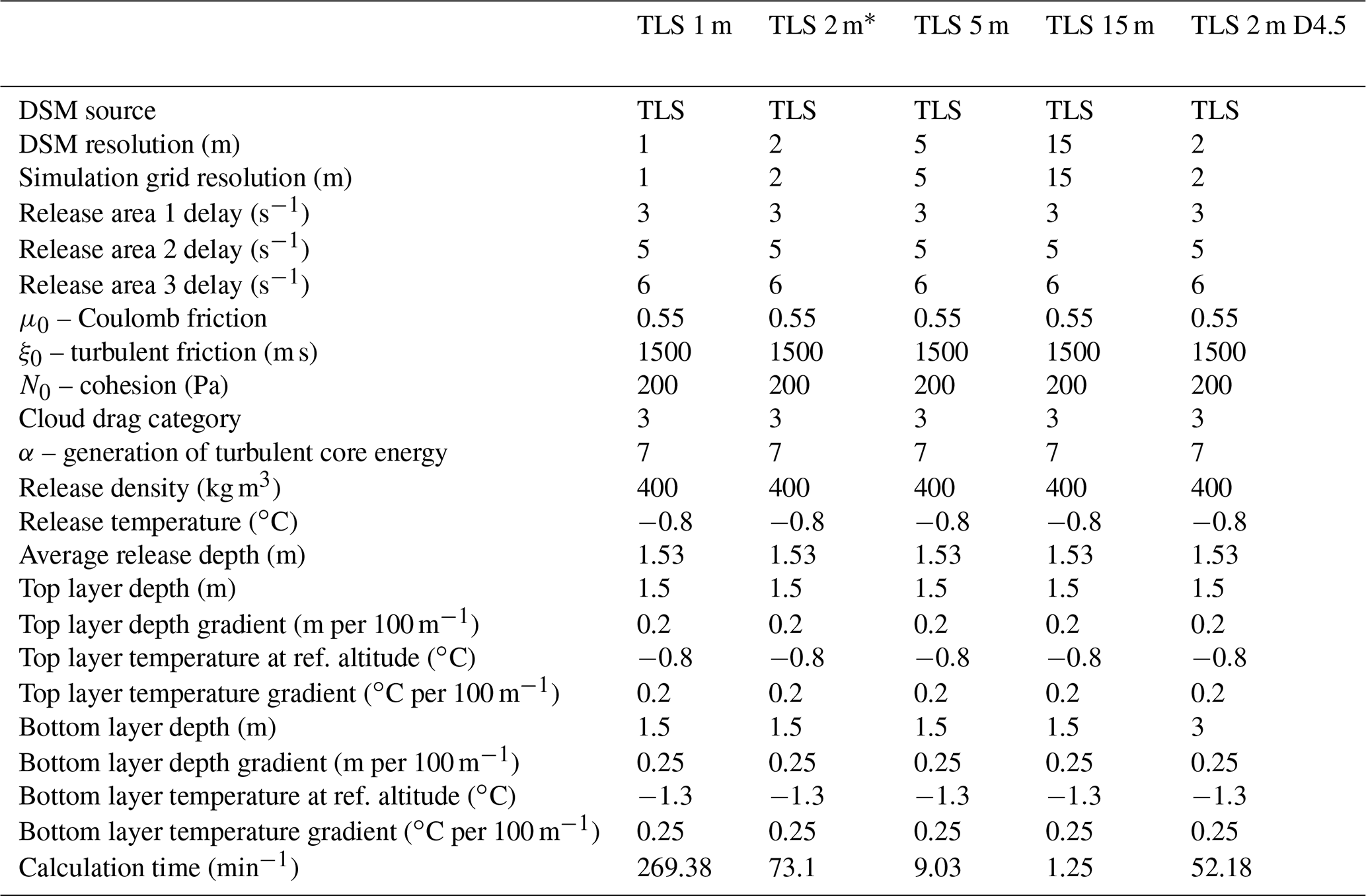
* Reference simulation calibrated against avalanche event documentation
Table A2RAMMS simulations performed with DSMs derived from satellite photogrammetric mapping (SPM) and the NZSoSDEM for the McPherson avalanche. The friction and entrainment parameters were held constant for each simulation, matching the reference TLS 2 m simulation, with the exception of SPM 2 m D4.5, which increased the bottom layer snow depth to simulate additional snow available for entrainment in the path. The release area delays are based on time from explosive charge detonation.
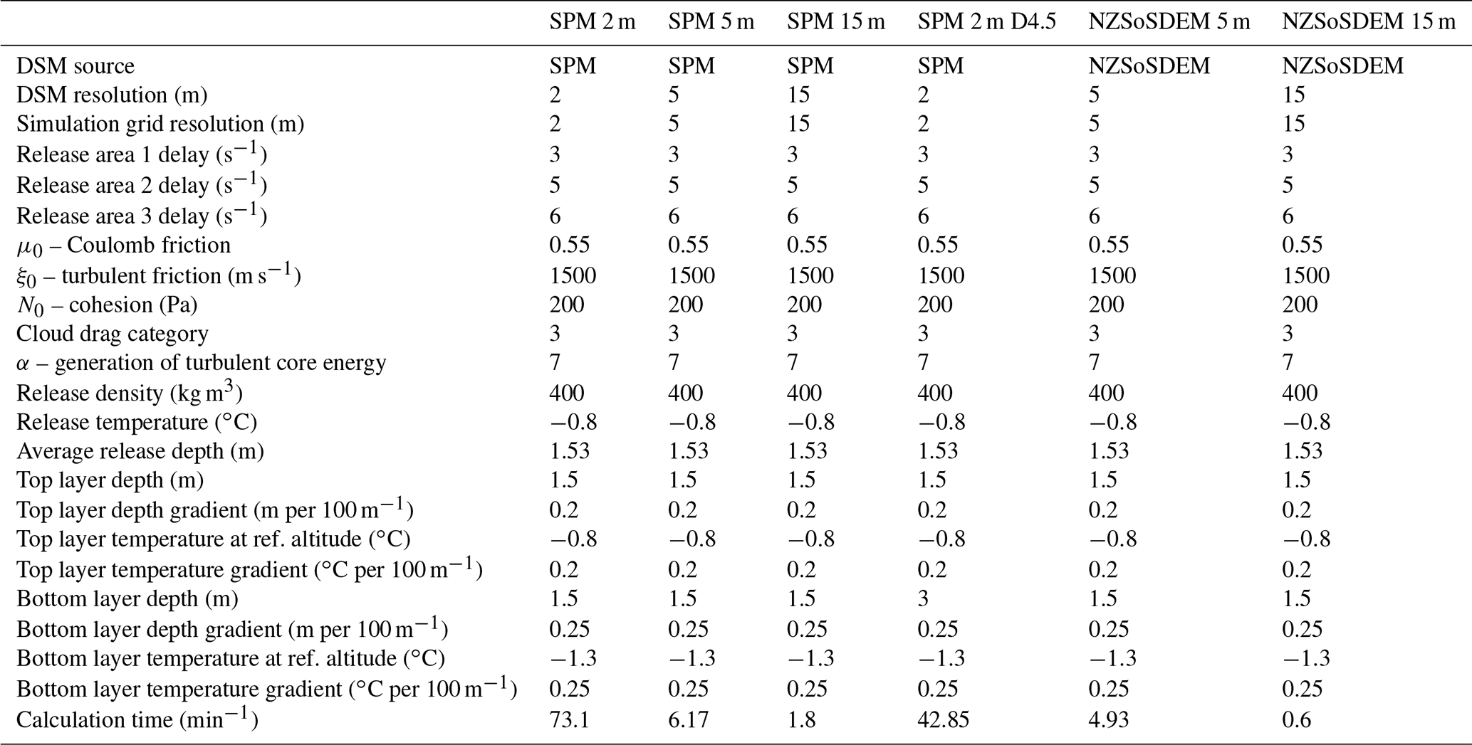
We used Ames Stereo Pipeline v2.7 to process the satellite imagery and interpolate the DSMs (DOI for v2.7: https://doi.org/10.5281/zenodo.3963341; Beyer et al., 2020).
Results of the RAMMS analysis can be viewed in an interactive map (Mountain Research Centre, 2022). Contact the corresponding author for more information on access to datasets.
AM, PS and YB conceived of the study. AM, SM, PS, TR and KT contributed to data collection. AM and PS processed the satellite imagery. SM and AM processed the lidar point clouds. AM and PB performed the RAMMS simulations with input from YB. AM, SM and TR prepared the manuscript with contributions from all co-authors. PS, NC and YB supervised the research.
At least one of the (co-)authors is a member of the editorial board of Natural Hazards and Earth System Sciences. The peer-review process was guided by an independent editor, and the authors also have no other competing interests to declare.
Publisher's note: Copernicus Publications remains neutral with regard to jurisdictional claims in published maps and institutional affiliations.
This research was supported by New Zealand Ministry of Business, Innovation and Employment through the Endeavour Smart Ideas research project “Quantifying environmental resources through high-resolution, automated, satellite mapping of landscape change” (grant no. UOOX1914). We would like to thank Downer NZ Ltd. Milford Road Alliance for logistical support for fieldwork and providing the lidar data. We would like to thank Etienne Berthier at LEGOS and the French space agency (CNES) for the use of the satellite imagery made available through the Pléiades Glacier Observatory (PGO) initiative. This paper contains © CNES (2020) and Airbus DS (2020) information, all rights reserved; commercial uses are forbidden. We thank the editor and two reviewers for constructive feedback that improved the manuscript.
This research has been supported by the Ministry of Business, Innovation and Employment (grant no. UOOX1914).
This paper was edited by Sven Fuchs and reviewed by two anonymous referees.
Aguilar, M. A., del Mar Saldana, M., and Aguilar, F. J.: Generation and Quality Assessment of Stereo-Extracted DSM From GeoEye-1 and WorldView-2 Imagery, IEEE T. Geosci. Remote, 52, 1259–1271, https://doi.org/10.1109/tgrs.2013.2249521, 2014. a
Airbus: Pléiades Imagery User Guide, Airbus Defence and Space Intelligence, https://www.intelligence-airbusds.com/automne/api/docs/v1.0/document/download/ZG9jdXRoZXF1ZS1kb2N1bWVudC01NTY0Mw==/ZG9jdXRoZXF1ZS1maWxlLTU1NjQy/airbus-pleiades-imagery-user-guide-15042021.pdf (last access: 19 August 2022), 2021. a
Allen, S. K., Schneider, D., and Owens, I. F.: First approaches towards modelling glacial hazards in the Mount Cook region of New Zealand's Southern Alps, Nat. Hazards Earth Syst. Sci., 9, 481–499, https://doi.org/10.5194/nhess-9-481-2009, 2009. a
Badoux, A., Andres, N., Techel, F., and Hegg, C.: Natural hazard fatalities in Switzerland from 1946 to 2015, Nat. Hazards Earth Syst. Sci., 16, 2747–2768, https://doi.org/10.5194/nhess-16-2747-2016, 2016. a
Baggio, T., Mergili, M., and D'Agostino, V.: Advances in the simulation of debris flow erosion: The case study of the Rio Gere (Italy) event of the 4th August 2017, Geomorphology, 381, 107664, https://doi.org/10.1016/j.geomorph.2021.107664, 2021. a
Bartelt, P., Salm, B., and Gruber, U.: Calculating dense-snow avalanche runout using a Voellmy-fluid model with active/passive longitudinal straining, J. Glaciol., 45, 242–254, https://doi.org/10.3189/s002214300000174x, 1999. a
Bartelt, P., Bühler, Y., Buser, O., Christen, M., and Meier, L.: Modeling mass-dependent flow regime transitions to predict the stopping and depositional behavior of snow avalanches, J. Geophys. Res.-Earth, 117, F01015, https://doi.org/10.1029/2010jf001957, 2012. a
Bartelt, P., Valero, C. V., Feistl, T., Christen, M., Bühler, Y., and Buser, O.: Modelling cohesion in snow avalanche flow, J. Glaciol., 61, 837–850, https://doi.org/10.3189/2015jog14j126, 2015. a
Bartelt, P., Buser, O., Valero, C. V., and Bühler, Y.: Configurational energy and the formation of mixed flowing/powder snow and ice avalanches, Ann. Glaciol., 57, 179–188, https://doi.org/10.3189/2016aog71a464, 2016. a, b, c
Bernard, T. G., Lague, D., and Steer, P.: Beyond 2D landslide inventories and their rollover: synoptic 3D inventories and volume from repeat lidar data, Earth Surf. Dynam., 9, 1013–1044, https://doi.org/10.5194/esurf-9-1013-2021, 2021. a
Berthier, E., Vincent, C., Magnússon, E., Gunnlaugsson, Á. Þ., Pitte, P., Meur, E. L., Masiokas, M., Ruiz, L., Pálsson, F., Belart, J. M. C., and Wagnon, P.: Glacier topography and elevation changes derived from Pléiades sub-meter stereo images, The Cryosphere, 8, 2275–2291, https://doi.org/10.5194/tc-8-2275-2014, 2014. a
Beyer, R., Alexandrov, O., McMichael, S., Broxton, M., Lundy, M., Husmann, K., Edwards, L., Nefian, A., Smith, B., Shean, D., Smith, T., mstyer, Annex, A., Moratto, Z., harguess, Aravkin, A., Meyer, J., Bhushan, S., and jlaura: NeoGeographyToolkit/StereoPipeline 2.7.0 (2.7.0), Zenodo [code], https://doi.org/10.5281/zenodo.3963341, 2020. a
Beyer, R. A., Alexandrov, O., and McMichael, S.: The Ames Stereo Pipeline: NASA's Open Source Software for Deriving and Processing Terrain Data, Earth Space Sci., 5, 537–548, https://doi.org/10.1029/2018ea000409, 2018. a, b
Bhushan, S., Shean, D., Alexandrov, O., and Henderson, S.: Automated digital elevation model (DEM) generation from very-high-resolution Planet SkySat triplet stereo and video imagery, ISPRS J. Photogram. Remote Sens., 173, 151–165, https://doi.org/10.1016/j.isprsjprs.2020.12.012, 2021. a
Blattner, P.: Geology of the crystalline basement between Milford Sound and the Hollyford Valley, New Zealand, NZ J. Geol. Geophys., 21, 33–47, https://doi.org/10.1080/00288306.1978.10420720, 1978. a
Bolstad, P. and Stowe, T.: An evaluation of DEM accuracy: elevation, slope, and aspect, Photogram. Eng. Remote Sens., 60, 1327–1332, 1994. a
Booth, A. M., McCarley, J. C., and Nelson, J.: Multi-year, three-dimensional landslide surface deformation from repeat lidar and response to precipitation: Mill Gulch earthflow, California, Landslides, 17, 1283–1296, https://doi.org/10.1007/s10346-020-01364-z, 2020. a
Bossi, G., Cavalli, M., Crema, S., Frigerio, S., Luna, B. Q., Mantovani, M., Marcato, G., Schenato, L., and Pasuto, A.: Multi-temporal LiDAR-DTMs as a tool for modelling a complex landslide: a case study in the Rotolon catchment (eastern Italian Alps), Nat. Hazards Earth Syst. Sci., 15, 715–722, https://doi.org/10.5194/nhess-15-715-2015, 2015. a
Bradshaw, J. Y.: Geology of crystalline rocks of northern Fiordland: Details of the granulite facies Western Fiordland Orthogneiss and associated rock units, NZ J. Geol. Geophys., 33, 465–484, https://doi.org/10.1080/00288306.1990.10425702, 1990. a
Brožová, N., Baggio, T., D'Agostino, V., Bühler, Y., and Bebi, P.: Multiscale analysis of surface roughness for the improvement of natural hazard modelling, Nat. Hazards Earth Syst. Sci., 21, 3539–3562, https://doi.org/10.5194/nhess-21-3539-2021, 2021. a, b, c, d, e, f, g
Bühler, Y., Christen, M., Kowalski, J., and Bartelt, P.: Sensitivity of snow avalanche simulations to digital elevation model quality and resolution, Ann. Glaciol., 52, 72–80, https://doi.org/10.3189/172756411797252121, 2011. a, b, c, d, e, f, g, h, i, j
Bühler, Y., Marty, M., and Ginzler, C.: High Resolution DEM Generation in High-Alpine Terrain Using Airborne Remote Sensing Techniques, T. GIS, 16, 635–647, https://doi.org/10.1111/j.1467-9671.2012.01331.x, 2012. a, b
Bühler, Y., Marty, M., Egli, L., Veitinger, J., Jonas, T., Thee, P., and Ginzler, C.: Snow depth mapping in high-alpine catchments using digital photogrammetry, The Cryosphere, 9, 229–243, https://doi.org/10.5194/tc-9-229-2015, 2015. a
Bühler, Y., Adams, M. S., Bösch, R., and Stoffel, A.: Mapping snow depth in alpine terrain with unmanned aerial systems (UASs): potential and limitations, The Cryosphere, 10, 1075–1088, https://doi.org/10.5194/tc-10-1075-2016, 2016. a, b
Bühler, Y., von Rickenbach, D., Stoffel, A., Margreth, S., Stoffel, L., and Christen, M.: Automated snow avalanche release area delineation – validation of existing algorithms and proposition of a new object-based approach for large-scale hazard indication mapping, Nat. Hazards Earth Syst. Sci., 18, 3235–3251, https://doi.org/10.5194/nhess-18-3235-2018, 2018. a
Bühler, Y., Bebi, P., Christen, M., Margreth, S., Stoffel, L., Stoffel, A., Marty, C., Schmucki, G., Caviezel, A., Kühne, R., Wohlwend, S., and Bartelt, P.: Automated avalanche hazard indication mapping on a statewide scale, Nat. Hazards Earth Syst. Sci., 22, 1825–1843, https://doi.org/10.5194/nhess-22-1825-2022, 2022. a, b
Buser, O. and Bartelt, P.: Production and decay of random kinetic energy in granular snow avalanches, J. Glaciology, 55, 3–12, https://doi.org/10.3189/002214309788608859, 2009. a
Buser, O. and Bartelt, P.: An energy-based method to calculate streamwise density variations in snow avalanches, J. Glaciol., 61, 563–575, https://doi.org/10.3189/2015jog14j054, 2015. a, b
Casteller, A., Christen, M., Villalba, R., Martínez, H., Stöckli, V., Leiva, J. C., and Bartelt, P.: Validating numerical simulations of snow avalanches using dendrochronology: the Cerro Ventana event in Northern Patagonia, Argentina, Nat. Hazards Earth Syst. Sci., 8, 433–443, https://doi.org/10.5194/nhess-8-433-2008, 2008. a
Christen, M., Bartelt, P., and Kowalski, J.: Back calculation of the In den Arelen avalanche with RAMMS: interpretation of model results, Ann. Glaciol., 51, 161–168, https://doi.org/10.3189/172756410791386553, 2010a. a, b, c, d, e, f, g
Christen, M., Kowalski, J., and Bartelt, P.: RAMMS: Numerical simulation of dense snow avalanches in three-dimensional terrain, Cold Reg. Sci. Technol., 63, 1–14, https://doi.org/10.1016/j.coldregions.2010.04.005, 2010b. a, b, c
Claessens, L., Heuvelink, G. B. M., Schoorl, J. M., and Veldkamp, A.: DEM resolution effects on shallow landslide hazard and soil redistribution modelling, Earth Surf. Proc. Land., 30, 461–477, https://doi.org/10.1002/esp.1155, 2005. a, b
Columbus, J., Sirguey, P., and Tenzer, R.: A free, fully assessed 15-m DEM for New Zealand, Surv. Quart., 66, 16–19, 2011. a, b, c, d
Courty, L. G., Soriano-Monzalvo, J. C., and Pedrozo-Acuña, A.: Evaluation of open-access global digital elevation models (AW3D30, SRTM, and ASTER) for flood modelling purposes, J. Flood Risk Manage., 12, e12550, https://doi.org/10.1111/jfr3.12550, 2019. a
Currier, W. R., Pflug, J., Mazzotti, G., Jonas, T., Deems, J. S., Bormann, K. J., Painter, T. H., Hiemstra, C. A., Gelvin, A., Uhlmann, Z., Spaete, L., Glenn, N. F., and Lundquist, J. D.: Comparing Aerial Lidar Observations With Terrestrial Lidar and Snow-Probe Transects From NASA's 2017 SnowEx Campaign, Water Resour. Res., 55, 6285–6294, https://doi.org/10.1029/2018wr024533, 2019. a
d'Angelo, P.: Improving semi-global mathing: Cost aggregation and confidence measure, Int. Arch. Photogram. Remote Sens. Spat. Inform. Sci., XLI-B1, 299–304, https://doi.org/10.5194/isprs-archives-xli-b1-299-2016, 2016. a
Deems, J. S., Painter, T. H., and Finnegan, D. C.: Lidar measurement of snow depth: a review, J. Glaciol., 59, 467–479, https://doi.org/10.3189/2013jog12j154, 2013. a
Deems, J. S., Gadomski, P. J., Vellone, D., Evanczyk, R., LeWinter, A. L., Birkeland, K. W., and Finnegan, D. C.: Mapping starting zone snow depth with a ground-based lidar to assist avalanche control and forecasting, Cold Reg. Sci. Technol., 120, 197–204, https://doi.org/10.1016/j.coldregions.2015.09.002, 2015. a
Dehecq, A., Gardner, A. S., Alexandrov, O., McMichael, S., Hugonnet, R., Shean, D., and Marty, M.: Automated Processing of Declassified KH-9 Hexagon Satellite Images for Global Elevation Change Analysis Since the 1970s, Front. in Earth Sci., 8, 566802, https://doi.org/10.3389/feart.2020.566802, 2020. a
Deschamps-Berger, C., Gascoin, S., Berthier, E., Deems, J., Gutmann, E., Dehecq, A., Shean, D., and Dumont, M.: Snow depth mapping from stereo satellite imagery in mountainous terrain: evaluation using airborne laser-scanning data, The Cryosphere, 14, 2925–2940, https://doi.org/10.5194/tc-14-2925-2020, 2020. a
Dowling, C. A. and Santi, P. M.: Debris flows and their toll on human life: a global analysis of debris-flow fatalities from 1950 to 2011, Nat. Hazards, 71, 203–227, https://doi.org/10.1007/s11069-013-0907-4, 2013. a
Dreier, L., Bühler, Y., Ginzler, C., and Bartelt, P.: Comparison of simulated powder snow avalanches with photogrammetric measurements, Ann. Glaciol., 57, 371–381, https://doi.org/10.3189/2016aog71a532, 2016. a
Eberhard, L. A., Sirguey, P., Miller, A., Marty, M., Schindler, K., Stoffel, A., and Bühler, Y.: Intercomparison of photogrammetric platforms for spatially continuous snow depth mapping, The Cryosphere, 15, 69–94, https://doi.org/10.5194/tc-15-69-2021, 2021. a, b, c, d, e, f, g, h, i
Fischer, J.-T., Kowalski, J., and Pudasaini, S.: Topographic curvature effects in applied avalanche modeling, Cold Reg. Sci. Technol., 74–75, 21–30, https://doi.org/10.1016/j.coldregions.2012.01.005, 2012. a
Fitzharris, B. and Owens, I.: Avalanche atlas of the Milford Road and an assessment of the hazard to traffic, Tech. rep., Report No. 4, NZ Mountain Safety Council, 79 pp., ISSN 0110-9499, 1980. a, b
Gao, J.: Resolution and accuracy of terrain representation by grid DEMs at a micro-scale, Int. J. Geogr. Informa. Sci., 11, 199–212, https://doi.org/10.1080/136588197242464, 1997. a, b
Grohmann, C. H., Smith, M. J., and Riccomini, C.: Multiscale Analysis of Topographic Surface Roughness in the Midland Valley, Scotland, IEEE T. Geosci. Remote, 49, 1200–1213, https://doi.org/10.1109/TGRS.2010.2053546, 2011. a
Hendrikx, J.: An examination of the snow and avalanche hazard on the Milford Road, Fiordland, New Zealand, PhD thesis, University of Canterbury, https://ir.canterbury.ac.nz/bitstream/handle/10092/1356/thesis_fulltext.pdf?sequence=2 (last access: 19 August 2022), 2005. a
Hergarten, S. and Robl, J.: Modelling rapid mass movements using the shallow water equations in Cartesian coordinates, Nat. Hazards Earth Syst. Sci., 15, 671–685, https://doi.org/10.5194/nhess-15-671-2015, 2015. a
Hirschmuller, H.: Stereo Processing by Semiglobal Matching and Mutual Information, IEEE T. Pattern Anal. Mach. Intel., 30, 328–341, https://doi.org/10.1109/tpami.2007.1166, 2008. a
Horton, P., Jaboyedoff, M., Rudaz, B., and Zimmermann, M.: Flow-R, a model for susceptibility mapping of debris flows and other gravitational hazards at a regional scale, Nat. Hazards Earth Syst. Sci., 13, 869–885, https://doi.org/10.5194/nhess-13-869-2013, 2013. a
Hungr, O. and McDougall, S.: Two numerical models for landslide dynamic analysis, Comput. Geosci., 35, 978–992, https://doi.org/10.1016/j.cageo.2007.12.003, 2009. a
Ivanova, K., Caviezel, A., Bühler, Y., and Bartelt, P.: Numerical modelling of turbulent geophysical flows using a hyperbolic shear shallow water model: Application to powder snow avalanches, Comput. Fluids, 233, 105211, https://doi.org/10.1016/j.compfluid.2021.105211, 2022. a
Kienzle, S.: The Effect of DEM Raster Resolution on First Order, Second Order and Compound Terrain Derivatives, T. GIS, 8, 83–111, https://doi.org/10.1111/j.1467-9671.2004.00169.x, 2003. a
Krishnan, S., Crosby, C., Nandigam, V., Phan, M., Cowart, C., Baru, C., and Arrowsmith, R.: OpenTopography, in: Proceedings of the 2nd International Conference on Computing for Geospatial Research & Applications – COM.Geo'11, ACM Press, https://doi.org/10.1145/1999320.1999327, 2011. a
Lague, D., Brodu, N., and Leroux, J.: Accurate 3D comparison of complex topography with terrestrial laser scanner: Application to the Rangitikei canyon (NZ), ISPRS J. Photogram. Remote Sens., 82, 10–26, https://doi.org/10.1016/j.isprsjprs.2013.04.009, 2013. a, b
Lassiter, H. A., Wilkinson, B., Perez, A. G., and Kelly, C.: Absolute 3D accuracy accessement of UAS LiDAR surveying, Int. Arch. Photogram. Remote Sens. Spat. Inform. Sci., XLIV-M-3-2021, 105–111, https://doi.org/10.5194/isprs-archives-xliv-m-3-2021-105-2021, 2021. a
Li, X., Sovilla, B., Jiang, C., and Gaume, J.: Three-dimensional and real-scale modeling of flow regimes in dense snow avalanches, Landslides, 18, 3393–3406, https://doi.org/10.1007/s10346-021-01692-8, 2021. a
Lin, Y.-C., Cheng, Y.-T., Zhou, T., Ravi, R., Hasheminasab, S. M., Flatt, J. E., Troy, C., and Habib, A.: Evaluation of UAV LiDAR for Mapping Coastal Environments, Remote Sens., 11, 2893, https://doi.org/10.3390/rs11242893, 2019. a
Macara, G.: The climate and weather of Southland, techreport 63, NIWA science and technology series, https://niwa.co.nz/static/Southland ClimateWEB.pdf (last access: 19 August 2022), 2013. a
Macara, G.: The climate and weather of Otago, 2nd Edn., techreport 67, NIWA science and technology series, https://docs.niwa.co.nz/library/public/NIWAsts67.pdf (last access: 19 August 2022), 2015. a
Maggioni, M., Bovet, E., Drier, L., Bühler, Y., Godone, D., Bartelt, P., Freppaz, M., Chiaia, B., and Segor, V.: Influence of summer and winter surface topography on numerical avalanche simulations, in: International snow science workshop proceedings 2013, Grenoble – Chamonix Mont Blanc, 591–598, https://www.dora.lib4ri.ch/wsl/islandora/object/wsl:16988 (last access: 19 August 2022), 2013. a, b, c, d, e
McClung, D. and Shaerer, P.: Snow avalanche size classification, in: International snow science workshop proceedings 1980, Vancouver BC, Canada, 12–30, https://arc.lib.montana.edu/snow-science/item/1202 (last access: 19 August 2022), 1980. a
Medina, V., Hürlimann, M., and Bateman, A.: Application of FLATModel, a 2D finite volume code, to debris flows in the northeastern part of the Iberian Peninsula, Landslides, 5, 127–142, 2008. a
Mergili, M.: r.avaflow – The mass flow simulation tool user manual v2.4, https://www.avaflow.org/manual.php (last access: 19 August 2022), 2020. a
Mergili, M., Fischer, J.-T., Krenn, J., and Pudasaini, S. P.: r.avaflow v1, an advanced open-source computational framework for the propagation and interaction of two-phase mass flows, Geosci. Model Dev., 10, 553–569, https://doi.org/10.5194/gmd-10-553-2017, 2017. a
Milford Opportunities Project: A Masterplan for Milford Sound Piopiotahi and the journey, https://www.milfordopportunities.nz/assets/Projects/210503-MOP-Masterplan-FINAL.pdf, last access: 3 May 2021. a
Moner, I., Orgué, S., Gavaldà, J., and Bacardit, M.: How big is big: results of the avalanche size classification survey, in: Interantional snow science workshop proceedings 2013, 242–246, https://arc.lib.montana.edu/snow-science/objects/ISSW13_paper_P1-05.pdf (last access: 19 August 2022), 2013. a
Mountain Research Centre: Interactive webmap of study results, ArcGIS Online [data set], https://arcg.is/0fqHS4, last access: 2 August 2022. a, b
Nolan, M., Larsen, C., and Sturm, M.: Mapping snow depth from manned aircraft on landscape scales at centimeter resolution using structure-from-motion photogrammetry, The Cryosphere, 9, 1445–1463, https://doi.org/10.5194/tc-9-1445-2015, 2015. a
Owens, I. and Fitzharris, B.: Avalanche atlas of the Milford Track and assessment of the hazard to walkers, Tech. rep., Report No. 8, NZ Mountain Safety Council, 77 pp., 1985. a
Planet Team: Planet Application Program Interface: In Space for Life on Earth, San Francisco, CA, https://api.planet.com/ (last access: 19 August 2022), 2020. a
Porter, C., Morin, P., Howat, I., Noh, M.-J., Bates, B., Peterman, K., Keesey, S., Schlenk, M., Gardiner, J., Tomko, K., Willis, M., Kelleher, C., Cloutier, M., Husby, E., Foga, S., Nakamura, H., Platson, M., Wethington, M., Williamson, C., Bauer, G., Enos, J., Arnold, G., Kramer, W., Becker, P., Doshi, A., D'Souza, C., Cummens, P., Laurier, F., and Bojesen, M.: ArcticDEM, Harvard Dataverse [data set], https://doi.org/10.7910/DVN/OHHUKH, 2018. a
Prokop, A.: Assessing the applicability of terrestrial laser scanning for spatial snow depth measurements, Cold Reg. Sci. Technol., 54, 155–163, https://doi.org/10.1016/j.coldregions.2008.07.002, 2008. a
Prokop, A., Schön, P., Singer, F., Pulfer, G., Naaim, M., Thibert, E., and Soruco, A.: Merging terrestrial laser scanning technology with photogrammetric and total station data for the determination of avalanche modeling parameters, Cold Reg. Sci. Technol., 110, 223–230, https://doi.org/10.1016/j.coldregions.2014.11.009, 2015. a, b, c
Rauter, M., Kofler, A., Huber, A., and Fellin, W.: faSavageHutterFOAM 1.0: depth-integrated simulation of dense snow avalanches on natural terrain with OpenFOAM, Geosci. Model Dev., 11, 2923–2939, https://doi.org/10.5194/gmd-11-2923-2018, 2018. a
Redpath, T. A. N., Sirguey, P., and Cullen, N. J.: Repeat mapping of snow depth across an alpine catchment with RPAS photogrammetry, The Cryosphere, 12, 3477–3497, https://doi.org/10.5194/tc-12-3477-2018, 2018. a
Reutebuch, S. E., Mcgaughey, R. J., Andersen, H.-E., Ward, W., and Carson, W. W.: Accuracy of a high-resolution lidar terrain model under a conifer forest canopy, Can. J. Remote Sens., 29, 527–535, https://doi.org/10.5589/m03-022, 2003. a
Reuter, H. I., Nelson, A., and Jarvis, A.: An evaluation of void-filling interpolation methods for SRTM data, Int. J.Geogr. Inform. Sci., 21, 983–1008, https://doi.org/10.1080/13658810601169899, 2007. a
Rickenmann, D., Laigle, D., McArdell, B. W., and Hübl, J.: Comparison of 2D debris-flow simulation models with field events, Comput. Geosci., 10, 241–264, https://doi.org/10.1007/s10596-005-9021-3, 2006. a
Rodríguez, E., Morris, C. S., and Belz, J. E.: A Global Assessment of the SRTM Performance, Photogram. Eng. Remote Sens., 72, 249–260, https://doi.org/10.14358/pers.72.3.249, 2006. a
Rusinkiewicz, S. and Levoy, M.: Efficient variants of the ICP algorithm, in: IEEE Proceedings third international conference on 3-D digital imaging and modeling, 145–152, https://doi.org/10.1109/IM.2001.924423, 2001. a
Sailer, R., Fellin, W., Fromm, R., Jörg, P., Rammer, L., Sampl, P., and Schaffhauser, A.: Snow avalanche mass-balance calculation and simulation-model verification, Ann. Glaciol., 48, 183–192, https://doi.org/10.3189/172756408784700707, 2008. a
Salm, B.: Contribution to avalanche dynamics, in: Symposium at Davos 1965 – Scientific Aspects of Snow and Ice Avalanches, Davos, Switzerland, 199–214, 1966. a
Sampl, P. and Zwinger, T.: Avalanche simulation with SAMOS, Ann. Glaciol., 38, 393–398, https://doi.org/10.3189/172756404781814780, 2004. a
Sappington, J. M., Longshore, K. M., and Thompson, D. B.: Quantifying landscape ruggedness for animal habitat analysis: A case study using bighorn sheep in the Mojave Desert, J. Wildlife Manage., 71, 1419–1426, https://doi.org/10.2193/2005-723, 2007. a, b
Schaerer, P.: The avalanche-hazard index, Ann. Glaciol., 13, 241–247, https://doi.org/10.3189/s0260305500007977, 1989. a
Shean, D. E., Alexandrov, O., Moratto, Z. M., Smith, B. E., Joughin, I. R., Porter, C., and Morin, P.: An automated, open-source pipeline for mass production of digital elevation models (DEMs) from very-high-resolution commercial stereo satellite imagery, ISPRS J. Photogram. Remote Sens., 116, 101–117, https://doi.org/10.1016/j.isprsjprs.2016.03.012, 2016. a, b, c, d
Shugar, D. H., Jacquemart, M., Shean, D., Bhushan, S., Upadhyay, K., Sattar, A., Schwanghart, W., McBride, S., de Vries, M. V. W., Mergili, M., Emmer, A., Deschamps-Berger, C., McDonnell, M., Bhambri, R., Allen, S., Berthier, E., Carrivick, J. L., Clague, J. J., Dokukin, M., Dunning, S. A., Frey, H., Gascoin, S., Haritashya, U. K., Huggel, C., Kääb, A., Kargel, J. S., Kavanaugh, J. L., Lacroix, P., Petley, D., Rupper, S., Azam, M. F., Cook, S. J., Dimri, A. P., Eriksson, M., Farinotti, D., Fiddes, J., Gnyawali, K. R., Harrison, S., Jha, M., Koppes, M., Kumar, A., Leinss, S., Majeed, U., Mal, S., Muhuri, A., Noetzli, J., Paul, F., Rashid, I., Sain, K., Steiner, J., Ugalde, F., Watson, C. S., and Westoby, M. J.: A massive rock and ice avalanche caused the 2021 disaster at Chamoli, Indian Himalaya, Science, 373, 300–306, https://doi.org/10.1126/science.abh4455, 2021. a
Simoni, A., Mammoliti, M., and Graf, C.: Performance of 2D debris flow simulation model RAMMS. Back-analysis of field events in Italian Alps., in: Conference Proceedings on 1st Annual International Conference on Geological & Earth Sciences, Global Science Technology Forum, https://doi.org/10.5176/2251-3361_geos12.59, 2012. a
Sirguey, P.: A Bivariate Thin-Plate Adaptive Smoothing Spline (BTPASS) to reduce noise in photogrammetric digital surface models, in: GeoComputation 2019, The University of Auckland, https://doi.org/10.17608/K6.AUCKLAND.9870014.V2, 2019. a
Sirguey, P. and Cullen, N.: A very high resolution DEM of Kilimanjaro via photogrammetry of GeoEye-1 images (KILISoSDEM2012), New Zealand Surveyor, 303, 19–215, 2014. a
Sommer, C. G., Lehning, M., and Mott, R.: Snow in a Very Steep Rock Face: Accumulation and Redistribution During and After a Snowfall Event, Front. Earth Sci., 3, 73, https://doi.org/10.3389/feart.2015.00073, 2015. a, b
Sovilla, B., McElwaine, J. N., Schaer, M., and Vallet, J.: Variation of deposition depth with slope angle in snow avalanches: Measurements from Vallée de la Sionne, J. Geophys. Res.-Earth, 115, F02016, https://doi.org/10.1029/2009jf001390, 2010. a, b
Stumpf, A., Malet, J.-P., Allemand, P., and Ulrich, P.: Surface reconstruction and landslide displacement measurements with Pléiades satellite images, ISPRS J. Photogram. Remote Sens., 95, 1–12, https://doi.org/10.1016/j.isprsjprs.2014.05.008, 2014. a
Takaku, J., Tadono, T., and Tsutsui, K.: Generation of High Resolution Global DSM from ALOS PRISM, Int. Arch. Photogram. Remote Sens. Spat. Inform. Sci., XL-4, 243–248, https://doi.org/10.5194/isprsarchives-xl-4-243-2014, 2014. a
Tarolli, P.: High-resolution topography for understanding Earth surface processes: Opportunities and challenges, Geomorphology, 216, 295–312, https://doi.org/10.1016/j.geomorph.2014.03.008, 2014. a, b
Techel, F., Jarry, F., Kronthaler, G., Mitterer, S., Nairz, P., Pavšek, M., Valt, M., and Darms, G.: Avalanche fatalities in the European Alps: long-term trends and statistics, Geogr. Helv., 71, 147–159, https://doi.org/10.5194/gh-71-147-2016, 2016. a
Thibert, E., Bellot, H., Ravanat, X., Ousset, F., Pulfer, G., Naaim, M., Hagenmuller, P., Naaim-Bouvet, F., Faug, T., Nishimura, K., Ito, Y., Baroudi, D., Prokop, A., Schön, P., Soruco, A., Vincent, C., Limam, A., and Héno, R.: The full-scale avalanche test-site at Lautaret Pass (French Alps), Cold Reg. Sci. Technol., 115, 30–41, https://doi.org/10.1016/j.coldregions.2015.03.005, 2015. a, b
Toitū Te Whenua/Land Information New Zealand: National Elevation Programme, Website, https://www.linz.govt.nz/data/linz-data/elevation-data, last access: 16 December 2021. a
Valero, C. V., Jones, K. W., Bühler, Y., and Bartelt, P.: Release temperature, snow-cover entrainment and the thermal flow regime of snow avalanches, J. Glaciol., 61, 173–184, https://doi.org/10.3189/2015jog14j117, 2015. a
Valero, C. V., Wever, N., Bühler, Y., Stoffel, L., Margreth, S., and Bartelt, P.: Modelling wet snow avalanche runout to assess road safety at a high-altitude mine in the central Andes, Nat. Hazards Earth Syst. Sci., 16, 2303–2323, https://doi.org/10.5194/nhess-16-2303-2016, 2016. a, b
van den Bout, B., van Asch, T., Hu, W., Tang, C. X., Mavrouli, O., Jetten, V. G., and van Westen, C. J.: Towards a model for structured mass movements: the OpenLISEM hazard model 2.0a, Geosci. Model Dev., 14, 1841–1864, https://doi.org/10.5194/gmd-14-1841-2021, 2021. a
Voellmy, A.: Uber die Zerstrungskraft von Lawinen, Schweizerische Bauzeitung, 73 pp. https://doi.org/10.5169/seals-61891, 1955. a
Waka Kotahi/NZ Transport Agency: Daily traffic counts, API, open data platform, https://opendata-nzta.opendata.arcgis.com/datasets/NZTA::tms-daily-traffic-counts-api/about (last access: 19 August 2022), 2021. a
Watson, L. M., Carpenter, B., Thompson, K., and Johnson, J. B.: Using local infrasound arrays to detect plunging snow avalanches along the Milford Road, New Zealand (Aotearoa), Nat. Hazards, https://doi.org/10.1007/s11069-021-05086-w, in press, 2021. a, b, c
Wessel, B., Huber, M., Wohlfart, C., Marschalk, U., Kosmann, D., and Roth, A.: Accuracy assessment of the global TanDEM-X Digital Elevation Model with GPS data, ISPRS J. Photogram. Remote Sens., 139, 171–182, https://doi.org/10.1016/j.isprsjprs.2018.02.017, 2018. a
Wheaton, J. M., Brasington, J., Darby, S. E., and Sear, D. A.: Accounting for uncertainty in DEMs from repeat topographic surveys: improved sediment budgets, Earth Surf. Proc. Land., 35, 136–156, https://doi.org/10.1002/esp.1886, 2009. a
Wise, S.: Assessing the quality for hydrological applications of digital elevation models derived from contours, Hydrol. Process., 14, 1909–1929, https://doi.org/10.1002/1099-1085(20000815/30)14:11/12<1909::aid-hyp45>3.0.co;2-6, 2000. a
Wood, B.: Geological map of New Zealand Sheet 27 Fiord, GNSScience, 1960. a
Wu, S., Li, J., and Huang, G.: A study on DEM-derived primary topographic attributes for hydrologic applications: Sensitivity to elevation data resolution, Appl. Geogr., 28, 210–223, https://doi.org/10.1016/j.apgeog.2008.02.006, 2008. a
Zhao, H. and Kowalski, J.: Topographic uncertainty quantification for flow-like landslide models via stochastic simulations, Nat. Hazards Earth Syst. Sci., 20, 1441–1461, https://doi.org/10.5194/nhess-20-1441-2020, 2020. a, b
Zugliani, D. and Rosatti, G.: TRENT2D: An accurate numerical approach to the simulation of two-dimensional dense snow avalanches in global coordinate systems, Cold Reg. Sci. Technol., 190, 103343, https://doi.org/10.1016/j.coldregions.2021.103343, 2021. a