Brief communication: Seismological analysis of flood dynamics and hydrologically triggered earthquake swarms associated with Storm Alex

On 2 October 2020, the Maritime Alps in southern France were struck by the devastating Storm Alex, which caused locally more than 600 mm of rain in less than 24 h. The extreme rainfall and flooding destroyed regional rain and stream gauges. That hinders our understanding of the spatial and temporal dynamics of rainfall–runoff processes during the storm. Here, we show that seismological observations from permanent seismic stations constrain these processes at a catchment scale. The analysis of seismic power, peak frequency, and the back azimuth provides us with the timing and velocity of the propagation of flash-flood waves associated with bedload-dominated phases of the flood on the Vésubie River. Moreover, the combined short-term average to long-term average ratio and template-matching earthquake detection reveal that 114 local earthquakes between local magnitude $M_{\mathrm{L}}=-\mathrm{0.5}$ and M_L=2 were triggered by the hydrological loading and/or the resulting in situ underground pore pressure increase. This study shows the impact of Storm Alex on the Earth's surface and deep-layer processes and paves the way for future works that can reveal further details of these processes.

1 Introduction

Extreme weather events might trigger an extreme response of the Earth's surface and subsurface processes, e.g., in the form of rapid and disastrous flash floods (e.g., Khajehei et al., 2020), mass movements (Stoffel and Huggel, 2012), and/or seismogenic underground stress changes (e.g., Rigo et al., 2008). These processes contribute to societal and environmental risks and are an important agent in landscape evolution. Moreover, some extreme weather events might become more frequent due to climate change (IPCC, 2022). That is why it is crucial to reliably quantify the spatio-temporal response of the Earth's systems to extreme weather forcing.

Seismic methods have the potential to monitor surface and subsurface processes associated with extreme weather events. In particular, both turbulent flow and sediment transport during floods generate ground motion in different frequency bands (Schmandt et al., 2013; Gimbert et al., 2014) that can be used to track the flood dynamics (e.g., Cook et al., 2018). Surface seismic waves are generated by impact forces exerted by mobile particles on the riverbed (e.g., Tsai et al., 2012; Gimbert et al., 2019), and ambient seismic measurements have recently been used to monitor fluxes associated with transported bed material (Bakker et al., 2020; Lagarde et al., 2021). In the past decade, near-river seismic monitoring has been conducted during moderate-magnitude floods (e.g., Burtin et al., 2016; Roth et al., 2016) and controlled small-magnitude flow events (Schmandt et al., 2013, 2017). To date, extensive seismic investigations of large-magnitude flood events are rare and mostly associated with glacier lake outburst floods (Cook et al., 2018; Maurer et al., 2020) and natural hazard cascade (Cook et al., 2021). Yet, improved understanding of flood dynamics is crucial for early warning, risk mitigation, and modeling landscape evolution (Raynaud et al., 2015; Borga et al., 2019).

Exceptionally intense rainfall can reactivate existing faults through changing crustal stress conditions due to additional fluid mass load or in situ stress changes, resulting in hydrologically triggered earthquakes (e.g., Hainzl et al., 2006). Over the past 2 decades, a growing number of studies have shown a correlation between meteorological events and earthquake activity in various geological contexts (Costain and Bollinger, 2010). Several sites show the seasonal modulation of the seismicity due to rainfall or snowmelt periods in Japan (Ueda and Kato, 2019); Nepal (Kundu et al., 2017); Taiwan (Hsu et al., 2021); Oregon, USA (Saar and Manga, 2003); California, USA (Johnson et al., 2017; Montgomery-Brown et al., 2019); and Italy (D'Agostino et al., 2018). Other observations display a transient increase in seismic activity following an exceptional rainfall episode, for example in the Swiss Alps (Roth et al., 1992), German Alps (Kraft et al., 2006), and southern France (Rigo et al., 2008).

Here, we present a set of seismological observations from 11 stations from the permanent French Résif network that captured the October 2020 extreme rainfall and flash flood caused by Storm Alex (Carrega and Michelot, 2021) in the southwestern Alps (the Maritime Alps), southeast France. This unique dataset allows us to study not only surface flash-flood-related hazard but also the seismogenic subsurface response to unusually intense rainfall which locally exceeded 600 mm in less than a day. Three rivers were strongly impacted by the flash floods: the Vésubie, the Roya, and the Tinée rivers (Fig. 1a). We first gain insights into the Vésubie River dynamics during the flash flood by analyzing seismic power, peak frequency, and dominant back-azimuthal orientation of seismic noise. These observations are compared with simple rainfall–runoff modeling (Brigode et al., 2021). Then, by using template matching, we detect a series of impulsive signals that correspond to small earthquakes (down to a local magnitude (M_L) of −0.5) in the area where the rainfall rate in the Tinée River catchment area was maximal. This preliminary analysis demonstrates that the seismological observations reported herein provide a better understanding and quantification of the hydro-geological impact of extreme weather phenomena on the mountainous terrain and the related fluvial hazards. The latter is important for catchment areas with few “classical” hydrological observations, such as the Vésubie River catchment presented here.

Figure 1 Study area, rainfall measurements, and recorded seismic data. (a) Study site and permanent Résif seismological stations superimposed over the total rainfall amount estimated by the ANTILOPE database (from 06:00 UTC on 2 October 2020 to 06:00 UTC on 3 October 2020). Background map source: © Google Maps 2021. The location of the earthquake swarms studied here is indicated by a purple star. The location in France of the study area is marked by a blue dot on the inset map. (b) The village of Saint-Martin-Vésubie before (summer 2020) and after the storm episode (source: IGN, 2020). (c) Annual maximum daily rainfall rate from the COMEPHORE database (hourly rainfall estimated on pixels of 1 km², available since 1997; Tabary et al., 2012) calculated over the 25 km² rectangle shown in Fig. B3a. (d) Vertical ground velocity at stations SPIF and TURF and vertical ground acceleration at station BELV filtered in 1–20 Hz (top) and their seismic power (bottom) recorded during 48 h, between 00:00 UTC on 2 October and 00:00 UTC on 4 October. The frequency axes are limited to 1–20 Hz.

2 Storm Alex – a very destructive Mediterranean episode

On 2 October 2020, the Maritime Alps were struck by a violent meteorological event called a “Mediterranean episode”, caused by Storm Alex (Carrega and Michelot, 2021). Although heavy rainfalls occur regularly in autumn in the Mediterranean region, the Storm Alex maximum daily rainfall was the highest that had occurred since the beginning of regional rainfall measurements in 1997. The continuous regional rainfall COMEPHORE database used in this study started in 1997 (Fig. 1c). The rainfall started at 06:00 UTC on 2 October 2020, lasted for less than 24 h, and generated a cumulative intensity that locally exceeded the typical yearly average (>600 mm d⁻¹, Fig. 1a). These estimates have been obtained hourly with ANTILOPE rainfall estimation (Laurantin, 2008) with a 1 km² spatial resolution. The ANTILOPE model was produced by Météo-France and constrained by radar data and 40 rain gauges located in the region (Fig. 1a). The locations of regional rain and stream gauges are shown in Fig. B1. The estimation of rainfall maps is highly uncertain in this context due to few rain gauges being available, rainfall measurement uncertainties due to observed intensities, limits of the radar observations, and spatial interpolation.

The torrential rains triggered hazardous flash floods and landslides of an intensity and spatial extent that had never been documented previously in this area, causing several casualties as well as large infrastructure and economic damage (Figs. 1a and B2; Brigode et al., 2021). To date, the spatial and temporal evolution of the flood remains poorly understood. This is partially due to a limited number of observations caused by instrument destruction during the flood. Stream gauge measurements during the episode are incomplete and highly uncertain due to scale saturation, destruction of measuring devices, and changes in the riverbed level.

We focus our flood-dynamics analysis on the Vésubie River because (1) the Vésubie catchment has been one of the most strongly affected in the region (Figs. 1, B2, and B3) and (2) the seismic station coverage is particularly suitable in this catchment with three seismic stations being located in proximity: SPIF (three-component velocimeter), BELV (three-component accelerometer), and TURF (three-component velocimeter) at about 1570, 630, and 5970 m, respectively, from the Vésubie River. We investigate the level of seismic power recorded by these stations by calculating the power spectral densities (PSDs; J. Solomon, 1991) during the storm. Then, we perform additional analysis on the SPIF station by assessing temporal changes in the (1) peak frequency, (2) dominant back-azimuthal orientation of seismic noise, and (3) relation between high-frequency (10–45 Hz) and low-frequency (1–10 Hz) seismic noise. We contextualize these seismological observations by comparing them with rainfall estimations obtained with the ANTILOPE model and runoff temporal series. The simple rainfall–runoff KLEM (Kinematic Local Excess Model; Borga et al., 2007) is used for runoff simulation. A full description of the methods used in this paper is provided in Appendix A.

3 Results

3.1 Seismological observations associated with the flash flood

All three seismic stations (SPIF, BELV, and TURF) show elevated noise levels during the 24 h period starting at 07:00 UTC on 2 October 2020 that overlap with the duration of Storm Alex (Carrega and Michelot, 2021) (Fig. 1d). The stations SPIF and BELV show elevated seismic power (PSD) from ∼ 10:00 UTC on 2 October to ∼ 06:00 UTC on 3 October in the frequency band 1–20 Hz. The seismic power during Storm Alex is at least 20 dB and up to about 30 dB higher than the pre-flood “background” ambient seismic noise power levels. Since the decibel scale is a base-10 logarithmic scale, a 20 dB observed difference means 100-times-higher seismic power. For the TURF station, the seismic power increased by at least 100 times relative to the pre-flood conditions, especially at frequencies lower than 5 Hz. The seismic power averaged in the 1–20 Hz frequency band for the SPIF and BELV stations (Fig. 2a and b) shows a rapid increase in recorded seismic power from 10:00 and 11:00 UTC, respectively. Three local seismic power maxima are visible at the SPIF and BELV stations. They are marked in color in Fig. 2, and the seismic power thresholds used to define the maxima are shown in Fig. B4. We determine the thresholds manually; they delimit the values in seismic power when the seismic power strongly and rapidly increases. The maxima 1 and 2 are not marked in Fig. 2c because we cannot identify them at the TURF station.

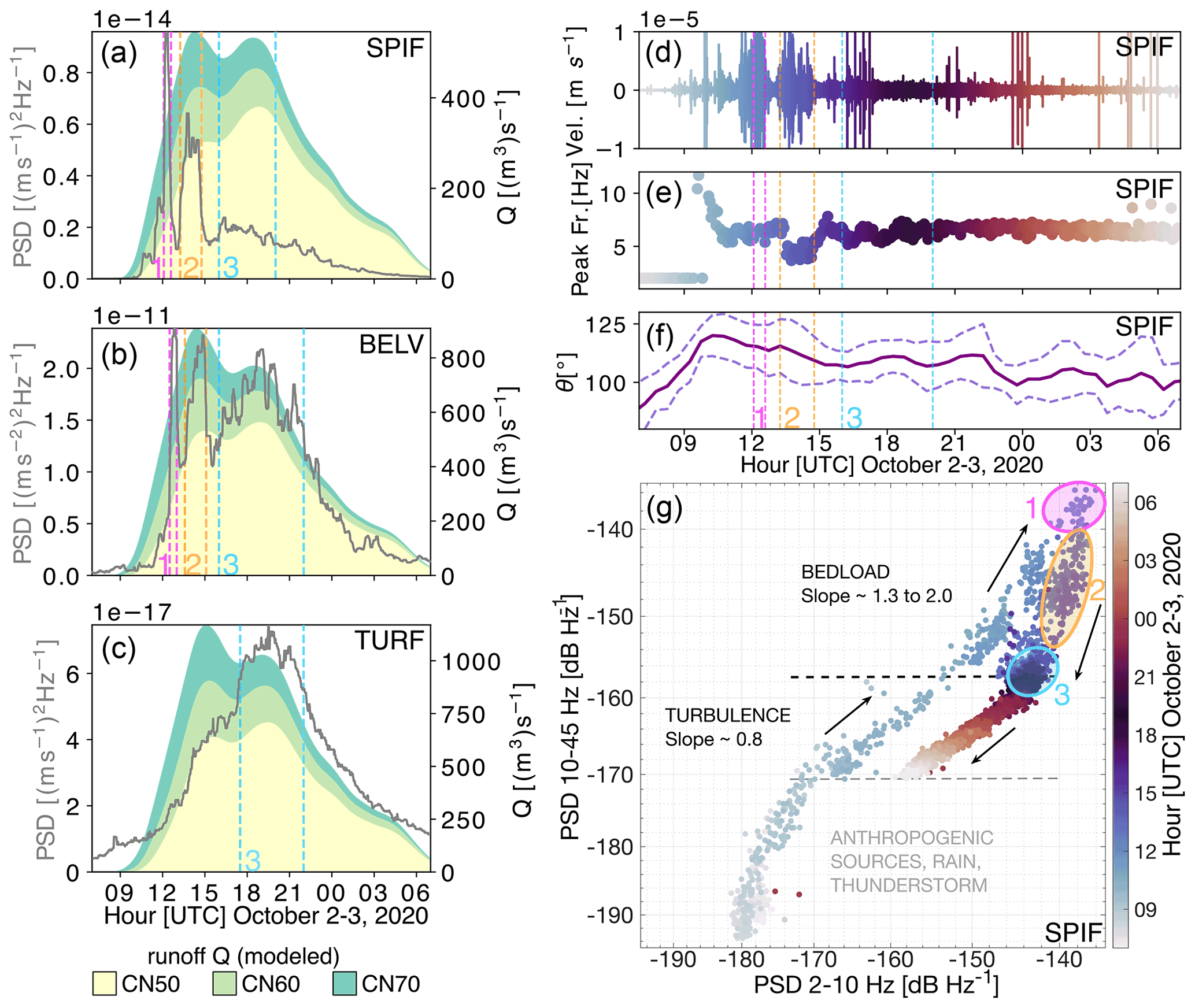
Figure 2 Analysis of continuous seismic signals recorded during Storm Alex. Seismic power (PSD) averaged between 1 and 20 Hz and recorded at stations (a) SPIF, (b) BELV, and (c) TURF. The results of the runoff simulation are marked in yellow (CN60), light green (CN70), and green (CN80), where CN denotes three different basin saturation scenarios: CN70 (moderate saturation), CN60, and CN50 (rather dry conditions). Seismic power is smoothed with a moving time window of 30 min, and the runoff is calculated with a 5 min time step. (d) Vertical ground velocity recorded at the SPIF station filtered in 1–50 Hz. (e) Peak frequency calculated for each 200 s segment. Peak frequency and the corresponding time segment are marked in the same color. (f) Back azimuth (smoothed over three consecutive 30 min time windows) calculated at the SPIF station averaged over 3–8 Hz and its standard deviations (dashed lines). (g) Seismic power in the 2–10 Hz frequency band versus seismic power in 10–45 Hz at the SPIF station. All results are shown from 07:00 UTC on 2 October to 07:00 UTC on 3 October 2020.

The first two seismic power maxima have pronounced high-amplitude peaks and arrive at 12:05 and 13:15 (SPIF), and 12:30 and 13:35 UTC (BELV). The third maximum has a distributed amplitude in time and occurs between ∼ 16:00 and ∼ 20:00 UTC at SPIF and ∼ 16:00 and ∼ 22:00 UTC at BELV.

The seismic power recorded at the TURF station shows a progressive increase with a single broad peak between ∼ 17:30 and ∼ 22:00 UTC. The peak associated with the first maximum has the highest magnitude at the SPIF station, while all three maxima have similar magnitudes at the BELV station. The peak associated with the first maximum lasts for ∼30 min, and that associated with the second maximum lasts for ∼90 min. The peak associated with the third maximum is the broadest, lasting for 4 and 6 h at the SPIF and BELV stations, respectively. For the sake of comparison with the runoff modeling, we use a linear scale for the seismic power representation in Figs. 2a and B4. For an alternative seismic power representation in decibels (10×log ₁₀ (PSD)), the reader can refer to Fig. B4.

Runoff simulations show two runoff maxima at three analyzed locations (Fig. 2a–c). The analyzed locations correspond to the river points with the shortest distance between the seismic stations and the Vésubie River and are shown in Fig. B3a. Modeling predictions indicate that the runoff maxima occur at 14:00, 14:25, and 15:00 UTC (the first runoff maximum) and 18:00, 18:25, and 19:00 UTC (the second runoff maximum), from upstream to downstream. The available stream gauge measurements at Utelle (Fig. B3a) show a similar rapid increase in runoff to the seismic power and the rainfall–runoff model (Fig. B5). However, no maximum runoff measurements are available since the stream gauge (marked as a dark-blue diamond in Figs. 1a and B3a) was destroyed during the flood.

To investigate potential changes in seismic noise sources, we calculate the peak frequency and the back azimuth (Fig. 2e and f). In Fig. 2e peak frequency values are color-coded by time, meaning that each color corresponds to the consecutive 200 s long time windows shown in Fig. 2a. The peak frequency corresponds to the frequency that has the maximum seismic power value in the analyzed time window (Fig. B6d). The peak frequency and back azimuth (θ, averaged in the 3–8 Hz frequency band, Fig. 2f) show a distinct value shift at the SPIF station before and during the flood. Starting from 08:30 UTC multiple lightning strikes occurred at a distance of 15 km from the SPIF station (https://www.blitzortung.org/en/, last access: 3 November 2020, Fig. B6). At this time there are higher-amplitude arrivals visible at the SPIF station causing jumps in the peak frequency from 2 Hz to higher values of up to 40–50 Hz at 09:30 UTC (Fig. B6). These arrivals can be associated with lightning and/or thunder, rain, or anthropogenic activity. However, at 11:00 UTC the peak frequency stabilizes at 6 Hz. Then, the peak frequency drops to 4 Hz at ∼ 13:20 UTC and comes back to 6 Hz at ∼ 15:00 UTC. This drop in the peak frequency coincides in time with the second seismic power maximum visible at the SPIF station. The back azimuth starts pointing along a 100–120^∘ axis at 10:00 UTC (Fig. 2f) although the degree of polarization is relatively weak (β²∼0.5, Fig. B7). The dominant degree of polarization (β² in the range 0–1), based on Koper and Hawley (2010), provides a measure for the confidence with which the horizontal azimuth can be interpreted, where β²>0.5 is recommended by Goodling et al. (2018). Therefore the back-azimuth observations should be taken with caution.

The relative contributions of low-frequency (2–10 Hz) and high-frequency (10–45 Hz) seismic power are shown in Fig. 2g. Different time periods characterized by a varying relationship between low-frequency and high-frequency seismic power can be identified: between 08:30 and 10:00 UTC the seismic power increases similarly in the two-frequency range (slope ∼ 1); between 10:00 and 16:00 UTC the high-frequency seismic power increases more strongly (slope > 1); and finally between 16:00 UTC on 2 October and 07:00 UTC on 3 October the seismic power decreases similarly. The equivalent of Fig. 2g on a linear amplitude scale ((m s⁻¹)² Hz⁻¹) is presented in Fig. B8. We discuss the significance of slope changes in the Discussion section.

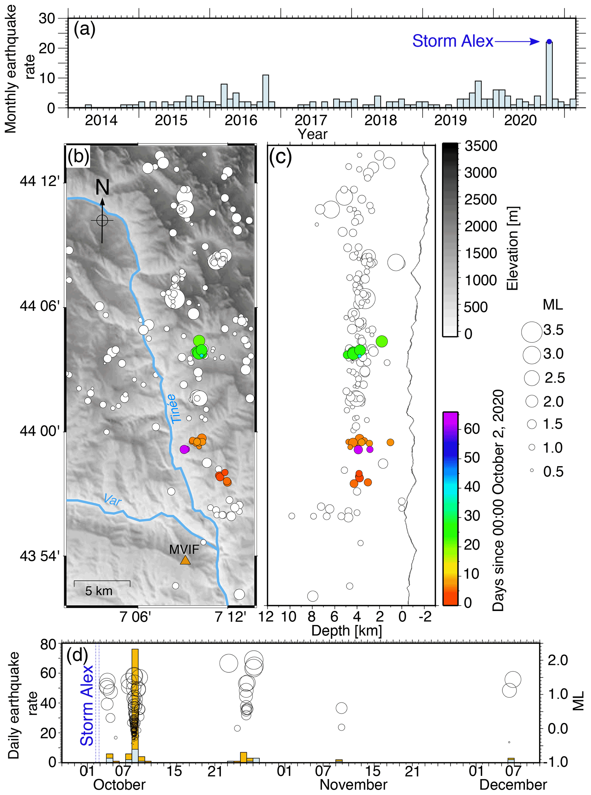
Figure 3 Seismic activity of the Tinée valley. (a) Monthly seismic activity between January 2014 and March 2021 detected by the SeisComP3 system. The blue arrow indicates the occurrence of Storm Alex. (b) Map of the seismicity over the period 2014–2021 located by the SeisComP3 system. Colored circles are earthquakes following Storm Alex. White circles are background seismicity. The orange triangle represents the seismological broadband station MVIF. (c) North–south cross section displaying the depth range of the seismicity with respect to the sea level and the line is the average elevation of the map in (b). (d) Daily rate (left axis) and local magnitude (right axis) for the seismic activity following Storm Alex. Gray bars are the number of earthquakes detected by the SeisComP3 system. The orange bars are the number of earthquakes detected by template matching. Black circles represent the detected earthquakes. The size is proportional to the magnitude. Dashed blue lines indicate the duration of Storm Alex.

3.2 Earthquake swarm detection

Since 2014, the seismic activity of the studied area is permanently monitored by the SeisComP3 (Hanka et al., 2010) system. A routine short-time average–long-time average (STA $/$ LTA) detection method is implemented in the SeisComP3 system, operating in Observatoire de la Côte d'Azur for the monitoring of the seismic activity in the southwestern Alps. For the past 7 years, the area of the Tinée valley has shown regular monthly seismic activity with an average of 2 earthquakes of local magnitude (M_L) larger than 0.4 and transient increases up to 11 earthquakes (Fig. 3). However, after Storm Alex, 23 earthquakes were detected, which is the highest monthly earthquake rate since 2014. This uncommon seismic activity consisted of 23 earthquakes located along the Tinée valley at around 4 km depth (Fig. 3b and c). The seismic crisis started on 4 October 2020, about 24 h after the end of Storm Alex, and lasted throughout October with small events in November and December (Fig. 3d). The earthquakes form three distinct swarms in space and time that were mostly successively activated from south to north (Fig. 3b and c). The location error is estimated to be about ±2 km. We detected 91 additional earthquakes by applying the template-matching detection method (Gibbons and Ringdal, 2006) to the continuous data recorded by the MVIF station (Fig. 3d). The template matching increases the number of detected earthquakes by about 400 % and decreases the minimum magnitude by 1 unit compared to the SeisComP3 detections based on STA $/$ LTA. Most of the newly identified events occurred on 8 October and may have been related to the central swarm since they best correlate with one of the templates constituting this cluster.

4 Discussion

4.1 The Vésubie River dynamics during the flash flood

Comparison among the increased seismic power (at least 100 and up to 1000 times larger than common noise levels), runoff modeling and runoff measurements indicates that the signals recorded by the SPIF, BELV, and TURF stations during Storm Alex are mostly generated by the flash flood on the Vésubie River. The rapid increase in seismic power, changes in peak frequencies, and dominant back azimuth suggest the flash flood on the Vésubie River started at about 10:00 UTC. The back-azimuth values measured at the SPIF station point towards the 110^∘ direction (Fig. B3, black arrow), which does not point towards the closest river section (located at a back azimuth of 66^∘). The back azimuth of ∼110^∘ may be associated with a bending of the Vésubie River channel, a ∼2.5 km long downstream reach of the Vésubie River that aligns with the estimated azimuth, or the confluence of the Venanson stream with the Vésubie River, which lies in the estimated direction (Fig. B3b). This provides evidence that the commonly made assumption that the recorded seismic signals are associated with the river segments located closest to the station (e.g., Roth et al., 2016; Zhang et al., 2021) may not always be valid.

Both seismic power and peak frequency are site-dependent seismic parameters; i.e., they depend on the seismic quality factor, the velocity of Rayleigh waves, and the source-station distance (Aki and Richards, 2002). However, according to a modified Tsai et al. (2012) model for hazardous flow monitoring from Lai et al. (2018), the seismic power is strongly sensitive to particle sediment size and flow speed, while the peak frequency mostly depends on the distance from the seismic source to the receiver. Also, previous observations reported no significant shift in peak frequency with varying runoff (Schmandt et al., 2013; Burtin et al., 2016). Therefore, the observed drop in the peak frequency (down to 4 Hz) that temporally correlates with the occurrence of the second seismic power maximum at the SPIF station (Fig. 2a and e) can potentially be generated by a stronger, more distant source. Indeed, the flash flood impacted the adjacent hill slopes through undercutting and destabilization of the riverbanks, leading to bank, road, and bridge collapses and landslides distributed along the river network (Fig. B2). Another possible explanation could be a tributary that becomes a dominant seismic source at this moment. However, the results of the rainfall–runoff modeling for large tributaries (the Boréon and Madone de Fenestre rivers) do not confirm this hypothesis. Also, the back-azimuth analysis does not show value changes during the second seismic power maximum. This can be due to (1) changes in the seismic source location that lie in the same general azimuthal direction; (2) the difference in timescale between back-azimuth estimates made over 30 min versus peak frequency calculations made over 200 s windows; or, perhaps most likely, (3) the low degree of polarization of the surface waves due to spatial spread of the source or to wave scattering.

Since river flow turbulence is expected to preferentially generate ground motion at low frequencies compared to bedload transport (e.g., Burtin et al., 2011; Schmandt et al., 2013; Gimbert et al., 2014), the relationships between seismic power at low versus high frequencies can tell us whether our observations may be sensitive to bedload transport (Bakker et al., 2020). As the flood develops we observe a change in scaling between low- and high-frequency seismic power, materialized by a transition from a 0.8 to a 1.3 scaling exponent as high-frequency seismic power becomes higher than −158 dB (Fig. 2g). We interpret this observation as an indication that high-frequency seismic power above the −158 dB threshold is mostly bedload induced. This is consistent with the expectation of enhanced bedload transport from this stage onwards due to increased bed shear stress and/or the activation of additional sediment supply sources from riverbed destabilization or bank erosion (Cook et al., 2018). Interestingly, after peak seismic energy has been reached, high-frequency seismic power drops drastically compared to low-frequency seismic power (with a scaling exponent of about 2), consistent with an abrupt decrease in sediment transport. Next, the low- versus high-frequency power scaling relation comes back to that observed during the early rising phase, consistent with higher frequencies over this time frame getting back to being mostly sensitive to water flow. We also note that after the flood, the low-frequency seismic power is higher compared to before the flood (∼10 dB difference; see also the spectrogram of the SPIF station in Fig. 1), which could be due to flood-induced changes in riverbed geometry and/or flow conditions (e.g., river roughness; Roth et al., 2017) that may preferentially affect low-frequency power.

About 6 h passed between the beginning of Storm Alex and the first flash-flood peak flow. The two seismic power maxima visible at the near-river stations (SPIF and BELV; the first maximum is marked in pink and the second one in orange in Fig. 2a, b, and g) occurred in what we identified as the bedload transport phase in Fig. 2g. Under the hypothesis that the two peaks associated with seismic power maxima represent the same moving source, we estimate their propagation velocity at 5.8 (±1.2) and 4.8 (±1.5) m s⁻¹, respectively. The details of the velocity and the error propagation calculation are given in Appendix B. These peaks overlap in time with the first maximum of runoff simulations (Fig. 2a and b). Such elevated and short-lived peaks could be generated by flood waves. Similar peaks in seismic power generated by flood waves were observed during glacial lake outburst floods in the Himalayas by Cook et al. (2018) and Maurer et al. (2020). These peaks may also be associated with the passage of sediment pulses such as those experimentally investigated by Piantini et al. (2021) in a torrential river setting. Such pulses can be generated by external sediment inputs to the river, triggered by the sudden destabilization of debris deposits at the base of slopes and cliffs.

The absence of the two main maxima on the TURF station can be related to a lack of sensitivity of this station to the bedload transport due to its large distance from the river (∼6 km). Farther distance means stronger geometrical attenuation at higher frequencies versus lower frequencies and thus lower sensitivity to bedload compared to water flow (Gimbert et al., 2014). Also, this station samples a longer river segment because of its farther distance, which could smooth out moving peaks. Moreover, due to the location of the TURF station further to the east, this station can also be influenced by the flood on the Roya River that is located ∼10 km away from the station. The timing of the main seismic power maximum at the TURF station and the third seismic power maximum of the BELV station are well correlated with the runoff simulations and can be related to the maximum runoff. From maxima 1 to 3, there is a shift from short-lived peaks to a much more spread out distribution of power through time. That could be potentially related to different dynamics of the first two maxima (associated with two fast-propagating flood waves causing a sudden rise in seismic power) and a progressive increase in the seismic power associated with a progressive increase in the runoff. Finally, the differences between the observed seismic power and the runoff simulations indicate that the simple runoff simulation cannot fully explain the flash-flood dynamics. In future works, seismic observations can provide additional constraints for more accurate rainfall–runoff simulations needed to further investigate the spatio-temporal dynamics of flash floods.

4.2 Earthquake swarm in the Tinée valley

The spatial coincidence between the maximum rainfall of Storm Alex in the Tinée valley and the seismic sequence a few hours later (Fig. 1a) raises the question of whether the earthquakes were triggered by the heavy rainfall. Three different hypotheses can be proposed for the triggering of seismicity by meteorological forcing. The first hypothesis is a pore pressure increase at depth caused by fluid migration from the surface through hydraulically connected fractures. In this case, the time lag between rainfall at the surface and earthquakes at depth is dependent on the hydraulic diffusivity along with the fractures (Saar and Manga, 2003; Kraft et al., 2006). The second hypothesis is an elastic stress perturbation in the crust induced by hydrological loadings, such as groundwater level increase after rainfall (Rigo et al., 2008). The third hypothesis is a pore pressure increase in deep fluid-saturated poroelastic rocks in response to overlying hydrological loading (Miller, 2008; D'Agostino et al., 2018).

The time lag between the onset of the rain (2 October, 06:00 UTC) and the onset of the first earthquake swarm (4 October, 00:52 UTC, southern swarm) is Δt=43 h. Taking a seismicity depth of z=5000 m ± 2000 m below the surface and using a time–distance-dependent equation for a propagating pore pressure front, $z=\sqrt{\mathrm{4}\mathit{\pi }D\mathrm{\Delta }t}$ (Shapiro et al., 1997), we find a hydraulic diffusivity ranging from D=4.6 to D=25.2 m² s⁻¹. This diffusivity range is unrealistically large to indicate earthquakes triggered by fluid migration. Indeed, with such a mechanism, earthquake activity following exceptional rainfall episodes or snowmelt is characterized by a delay of several days to several months and a lower hydraulic diffusivity ranging from D=0.01 to D=5.00 m² s⁻¹ (Kraft et al., 2006; Saar and Manga, 2003; Husen et al., 2007; Montgomery-Brown et al., 2019). Thus, the first hypothesis is unlikely for the first earthquake swarm.

The geology of the Tinée valley consists of limestone formations topped by a sandstone layer (Grès d'Annot). These rocks can store large volumes of water, which might support the hypothesis of seismicity triggered by groundwater weight. Rigo et al. (2008) describe earthquake triggering in a karstic (made up of limestone) region at depths smaller than 10 km, 43 h after the onset of heavy rainfall. The authors interpret this earthquake activity as the response of the crust to an elastic stress increase caused by vertical loading because of the groundwater level rise. On the other hand, Miller (2008) shows that a sharp increase in the hydraulic loading in karst can also produce an instantaneous increase in the pore pressure in the underlying fluid-saturated crust, able to trigger earthquakes.

The resumption of activity of the southern swarm at the same time as the activation of the central swarm (6 d after Storm Alex) and the activation of the northern swarm (22 d after Storm Alex) is more compatible with surface-to-depth fluid migration. However, as these swarms are at the same depth, this would imply a rather large spatial variation in the hydraulic diffusivity from D=1.4 to D=7.5 m² s⁻¹ for the southern and central swarms to D=0.4 to D=2.0 m² s⁻¹ for the northern swarm. The successive activation of the three swarms could also suggest an alternative mechanism of triggered seismicity. The northward migration of the seismicity is around 20–30 m h⁻¹. This velocity is much greater than 1–10 m d⁻¹, usually attributed to fluid diffusion-driven seismicity (e.g., Chen et al., 2012; Ruhl et al., 2016). Yet, this velocity is also lower than velocities reported for aseismic slip-driven seismicity (typically 100–1000 m h⁻¹; e.g., Lohman and McGuire, 2007; Roland and McGuire, 2009; Ruhl et al., 2016; Hatch et al., 2020). However, Chen and Shearer (2011) and Chen et al. (2012) also attribute slow earthquake migration of orders 10–100 m h⁻¹ to aseismic slip, which are values compatible with velocities we found. Hence the northward migration of the seismicity might highlight the horizontal propagation of an aseismic slip along a fault parallel to the valley. The overlying hydrological loading could trigger this aseismic slip, and its northward propagation could drive the successive rupture of seismic asperities corresponding to the three swarms. The interplay between hydromechanical and aseismic slip processes is increasingly recognized as a driver of earthquake swarms (e.g., de Barros et al., 2020; Hatch et al., 2020). Finally, the seismicity triggered by Storm Alex is collocated with the previous background seismicity, especially at depth (Fig. 3). This area of the southwestern Alps experiences regular moderate seismic activity. Therefore, the heavy rainfall has likely promoted ruptures on seismogenic structures that could have failed in the longer term. In future studies, measurements of relative seismic velocity changes ($dv/v$; e.g., Brenguier et al., 2008; Illien et al., 2022) could provide additional insights into the state of the subsurface before, during, and after the storm.

5 Conclusions

Our results show that seismometers can constrain interaction between the different Earth's systems, time- and space-dependent processes during the flood, and the rainfall–runoff relationship at the catchment scale. This is particularly important in the absence of traditional hydrological measurements, as in the study presented here. Observations from permanent seismological stations in the Maritime Alps provide the timing and velocity propagation of the flood waves. They reveal bedload- and turbulence-dominated phases of the flood that occurred on the Vésubie River. Our observations also suggest that 114 earthquakes between local magnitude M_L=0.5 and M_L=2.5 were triggered by the hydrological loading and/or by the resulting in situ pore pressure increase in the Tinée valley. Heavy rainfall occurs regularly in autumn in the Mediterranean region, and its intensity is increasing due to climate change (Tramblay and Somot, 2018; Ribes et al., 2019). In the future, installing spatially dense seismic arrays could help further detect and constrain the dynamics of floods and triggered earthquakes (e.g., Meng and Ben-Zion, 2017; Eibl et al., 2020; Chmiel et al., 2021). Finally, the results from this study pave the way for a more detailed analysis of surface and deep Earth processes associated with Storm Alex using the unique dataset presented.

Appendix A: Methods

A1 Seismic power calculation and peak frequency

Stations SPIF, BELV, and TURF are located 1570, 630, and 5970 m away, respectively, from the Vésubie River. SPIF and TURF are equipped with a three-component broadband (BB) velocimeter and a three-component accelerometer, and BELV is only equipped with a three-component accelerometer. On SPIF and TURF we use the BB recordings for the analysis because of the instrument's higher sensitivity than the accelerometer. The sampling frequency for the SPIF and TURF stations is 100 Hz and for the BELV station is 125 Hz. Stations BELV and TURF are affected by high-frequency noise that does not allow us to analyze signals higher than 20 Hz. To focus on river-generated seismic signals, we use high-frequency signals (1–50 Hz for the SPIF station and 1–20 Hz for BELV and TURF stations). After the removal of the instrumental response, we first calculate power spectral densities (PSDs), splitting the data into 200 s long time windows with a 50 % overlap (in Figs. 1d and 2a–c), but no overlap is used in Fig. 2e and g. The windowing function window is applied to each segment, and the PSD is calculated by Welch's average periodogram method (J. Solomon, 1991). Then for the SPIF station, we follow previous work on debris flows (Lai et al., 2018) and we investigate the signal's peak frequency in individual 200 s time windows between 2–50 Hz. We also analyze seismic power recorded at the SPIF station in two different frequencies bands: 2–10 and 10–45 Hz. For that, we estimate PSD using again Welch's method with time segments of 2 s and no overlap, and then we calculate a median over 30 s time windows.

A2 Azimuth analysis

We perform a frequency-dependent polarization analysis to determine the dominant back azimuth assuming that the seismic signature of the flood is dominated by surface waves at the SPIF station (Goodling et al., 2018). The horizontal azimuth and degree of polarization are determined based on the dominant eigenvector of the spectral covariance matrix of the three measured components (N, E, and Z), following the approach of Park et al. (2005) and its recent application by Goodling et al. (2018). We determine these variables for 30 min intervals using nine subwindows with 50 % overlap. The dominant azimuth per frequency (θ) is obtained and given for a range 0–180^∘ as there is a 180^∘ ambiguity in this value.

A3 Rainfall–runoff models

Runoff is firstly estimated using the Soil Conservation Service curve number (SCS-CN) production function method. The SCS-CN function allows us to estimate the runoff from a rainfall event depending on the catchment saturation conditions. A simplified unit hydrograph routing function is then used to produce temporal runoff series. This analysis aims at estimating, for each studied catchment, the distances between each digital elevation model (DEM) grid cell and the considered outlet and uses the distance to root the runoff at the studied catchment outlets. A distinction is made between the distance traveled on the slopes and the distance traveled in the river (i.e., within the hydrographic network): the flow velocity on the slopes (fixed here at 0.2 m s⁻¹) is assumed to be slower than that in the river (fixed here at 5 m s⁻¹). These distances are used to calculate, for each grid cell x belonging to a studied watershed, the transfer time τ (in seconds) between this grid cell x and the considered outlet:

$$\begin{array}{}\text{(A1)}& \mathit{\tau }\left(x\right)={\displaystyle \frac{L_h\left(x\right)}{v_h}}+{\displaystyle \frac{L_c\left(x\right)}{v_c}},\end{array}$$

where L_h(x) is the distance (on the slopes) between the grid cell x and the considered catchment outlet (m). v_h is the flow velocity on the slopes (m s⁻¹). L_c(x) is the distance (in the river network) between the grid cell x and the considered catchment outlet [m]. v_c is the flow velocity in the river network (m s⁻¹).

These transfer times are used to calculate the simulated flow, at time step t, at each studied outlet (denoted Q and expressed in m³ s⁻¹) by the following expression (no initial base flow is considered in this study):

$$\begin{array}{}\text{(A2)}& Q\left(t\right)=\underset{A}{\int }q(t-\mathit{\tau }(x),x)\mathrm{d}x,\end{array}$$

where A is the catchment area upstream of the grid cell x (km²). q is the runoff estimated at time step t and at the grid cell x (m s⁻¹). The runoff is simulated for three locations along the Vésubie River which are the closest to the seismic stations (Fig. B3).

A4 Earthquake swarm detection

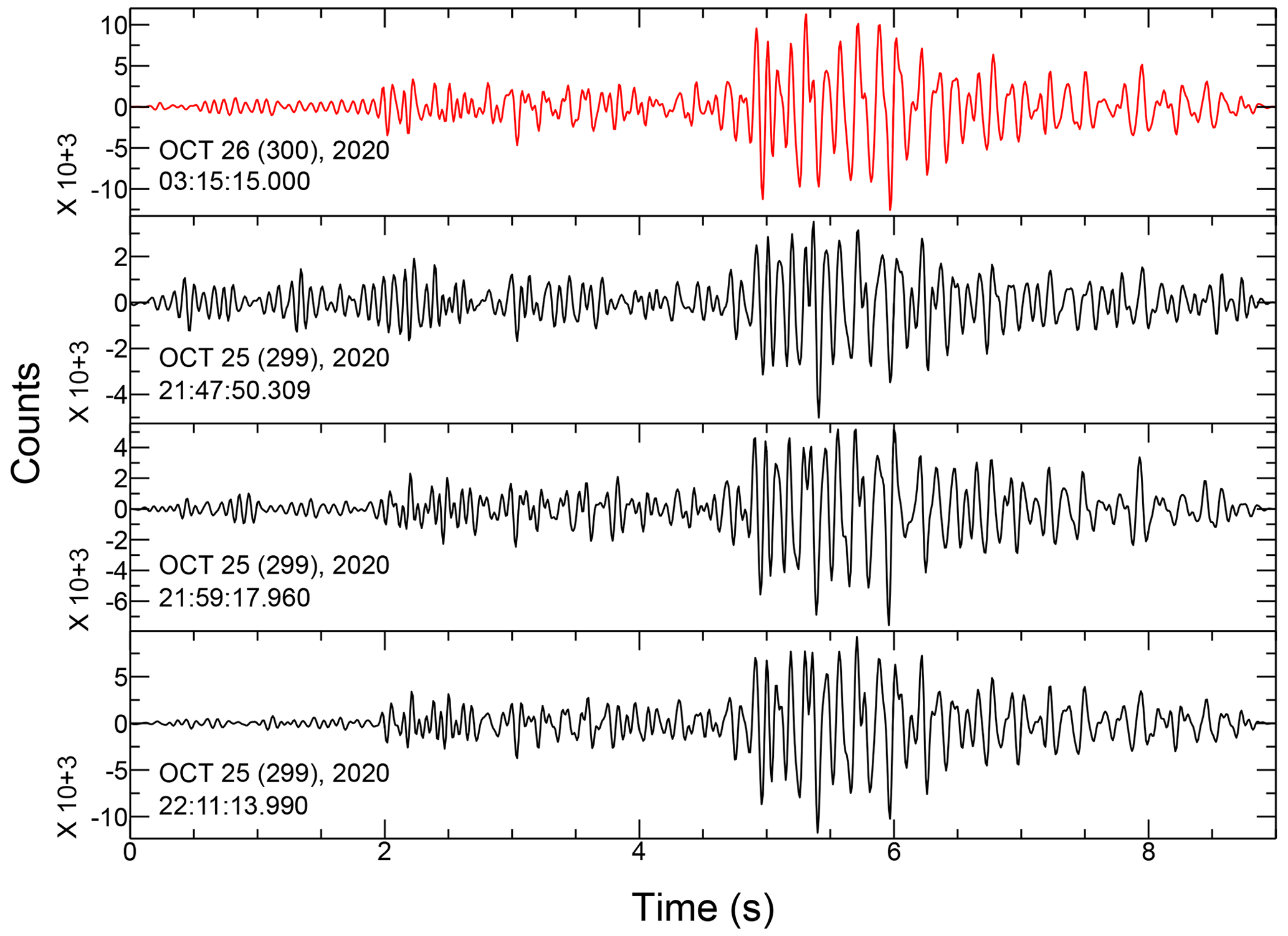
Previous studies have shown that template matching (e.g., Gibbons and Ringdal, 2006) has a higher detection sensitivity than threshold-based methods such as the STA $/$ LTA used in the SeisComP3 system. We use template matching to detect low-magnitude earthquakes that belong to the earthquake swarms. Template matching is performed at the broadband station MVIF (10 km to the south of the swarm). We verified that this station was little affected by the seismic noise generated by the increased river flow during and after the storm. We use the following approach. Data are bandpass-filtered in the 5–30 Hz frequency band. We use as templates the 23 earthquakes detected by SeisComP3. The templates are constructed using a 5 s window that includes P and S waves. Next, each template is cross-correlated with daily continuous seismic data. We use only vertical components of the seismograms, and we automatically scan the seismic data between 27 September and 10 December 2020. A new earthquake is detected if the cross-correlation coefficient exceeds a threshold of 0.6. This value allows the detection of earthquake waveforms that might slightly differ from the templates (if, for example, the origin location is not the same) while minimizing the number of false detections. Finally, the magnitude of detected earthquakes is estimated from the ratio between its maximum amplitude and the maximum amplitude of the best-correlated template (local magnitude M_L). An example of templates and detected events by template matching are presented in Figs. B10–B12.

A5 Peak propagation velocity and uncertainty calculation

The peak arrival times are manually picked by taking the beginning of the maximum above fixed seismic power (PSD) thresholds (Figs. B4 and B9). Also, we verify the time delay between the two PSDs using cross-correlation (Fig. B9). We find two maxima of 0.30 and 0.15 at time lag values of 19 and 28 min, respectively. We calculate the peak propagation velocity as a ratio between the distance (d) of the two nearest river coordinates to the SPIF and BELV stations (8012 m) to manually pick the propagation time of the peaks (t). To calculate the distance, we use the nearest river coordinates to the stations, and we integrate the distance following the Vésubie River coordinates (8012 m). Then, we use error propagation to estimate the uncertainty in the estimated velocity propagation. For that, we use the variance formula assuming that the distance and time measurements are independent:

$$\begin{array}{}\text{(A3)}& s_v=\sqrt{{\left(-{\displaystyle \frac{d}{t^{\mathrm{2}}}}\right)}^{\mathrm{2}}{s}_t^{\mathrm{2}}+{\left({\displaystyle \frac{\mathrm{1}}{t}}\right)}^{\mathrm{2}}{s}_d^{\mathrm{2}}},\end{array}$$

where d is the distance between the two nearest river coordinates to the SPIF and BELV stations (8012 m), t the manually picked propagation time of the peaks (s), s_t the standard deviation of the three propagation times (s) – (1) the manually picked propagation time of the peaks and (2) the two cross-correlation calculated propagation times – and s_d the standard deviation of the two distances (m) – (1) the distance between the nearest river coordinates to the SPIF and the BELV stations (8012 m) and (2) the distance of the closest river segment that aligns with the dominant back azimuth calculated at the SPIF station to the closest river coordinates to the BELV station (5512 m).

Appendix B: Supplemental figures

Figure B1 The location of rain and stream gauges and seismic stations in southeastern France. Background map source: © Google Maps 2021.

Figure B2 The consequences of Storm Alex in the Maritime Alps. (a) Landslide located upstream of the village of Saint-Martin-Vésubie on the right bank of the Boréon River. (b) Bank collapse next to the village of Saint-Martin-Vésubie. (c) Aerial view of the village of Roquebillière. (d) Partial bank collapse and deposited material next to the road in the commune of Roquebillière. Photo credits: Florent Adamo/Cerema.

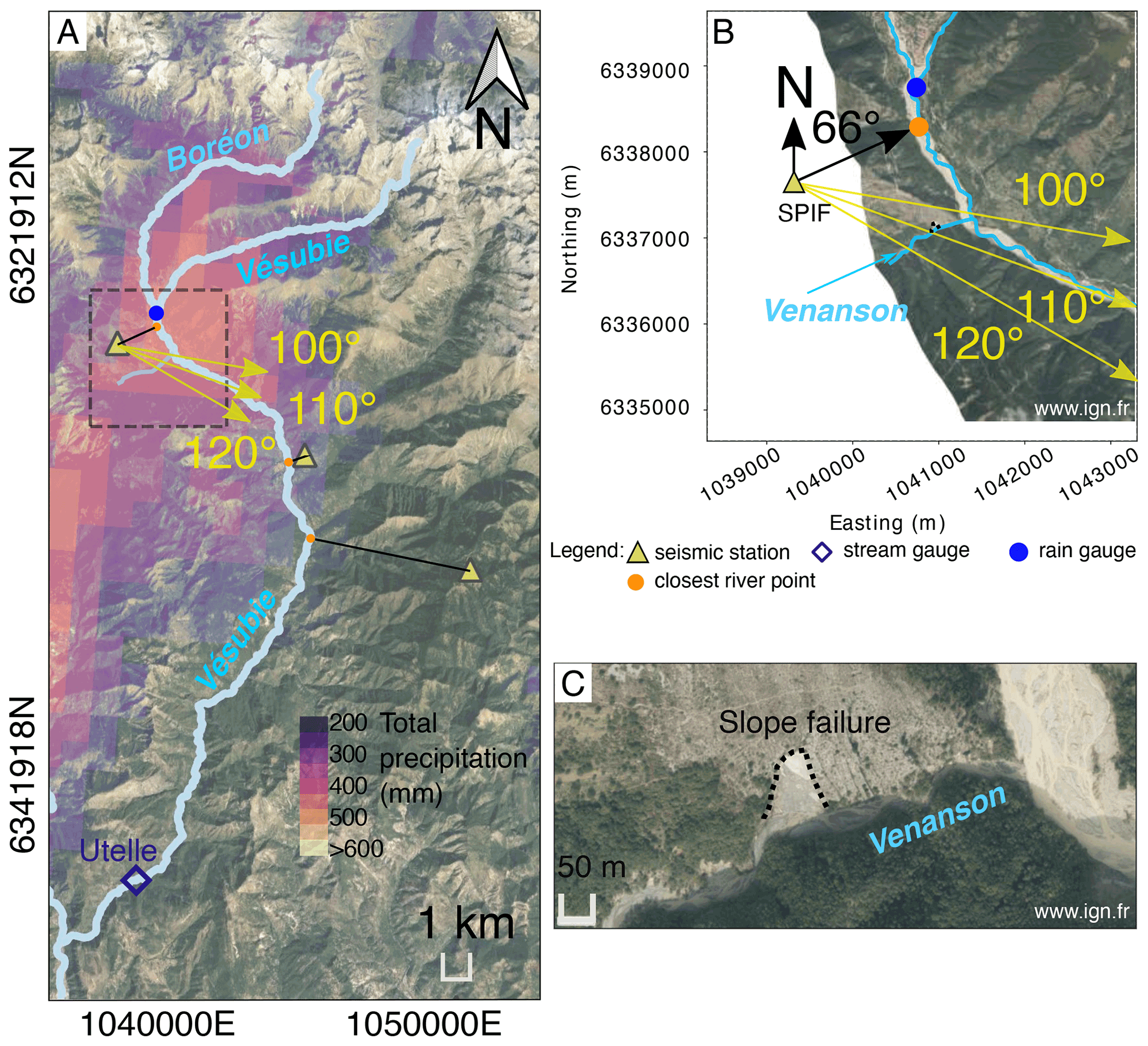
Figure B3 (a) Map section showing the Vésubie and the Boréon rivers. The 25 km² square used for the rainfall calculation in Fig. 1b is shown with dashed black lines. Background map source: © Google Maps 2021. (b) Zoomed-in view of the square marked in panel (a). Three dominant azimuths are indicated in yellow arrows, showing dominant noise directions of 100, 110, and 120^∘ (source: IGN, 2020). (c) Zoomed-in view of the intersection between the Venanson stream and the Vésubie River, with a slope failure indicated that is adjacent to the Venanson stream (source: IGN, 2020).

Figure B4 Seismic power (PSD) recorded at SPIF, BELV, and TURF seismic stations on a linear scale (a, c, e) and logarithmic scale (dB; b, d, f). The seismic power is averaged in the 1–20 Hz frequency band, between 07:00 UTC on 2 October and 07:00 UTC on 3 October. Vertical lines show the starting hours of the three peaks, and the horizontal lines show the threshold used to define the peaks.

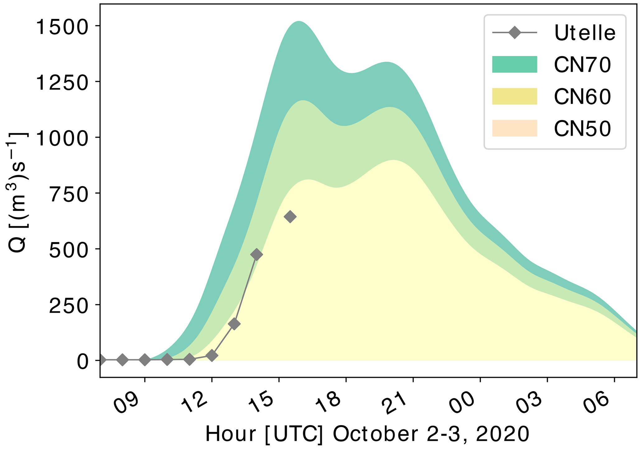
Figure B5 Runoff modeling for three different basin saturation scenarios: CN70 (moderate saturation), CN60, and CN50 (rather dry conditions). Available runoff measurements from the stream gauge at Utelle are presented in gray diamonds. The comparison between the stream gauge measurements and runoff modeling indicates rather dry basin conditions (CN50 scenario). However, there is an uncertainty in the runoff modeling related to the estimated flow velocities on the slope (0.2 m s⁻¹) and in the river (5.0 m s⁻¹). Moreover, the estimated runoff values are too low compared to the damage that occurred in the Vésubie catchment.

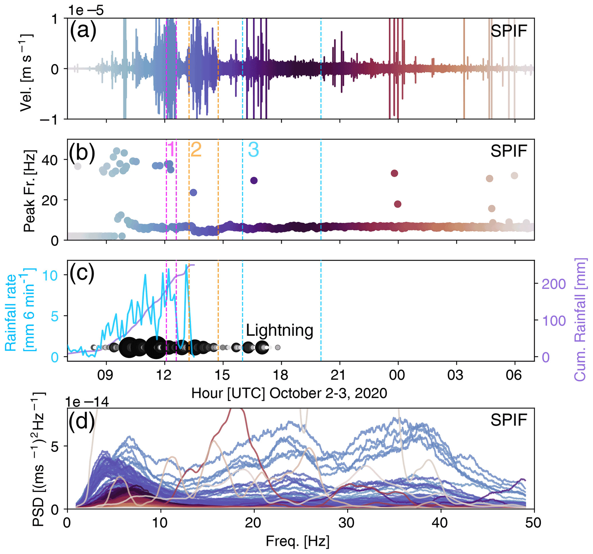
Figure B6 Analysis of seismic data recorded at the SPIF station and meteorological data. (a) Vertical ground velocity recorded filtered in 1–50 Hz. (b) Peak frequency calculated for each 200 s segment. (c) Rainfall measured by the rain gauge located at Saint-Martin-Vésubie. This is the closest rain gauge to the SPIF station located at a distance of 1.9 km. The measurement stopped when the instrument was destroyed. Lightning at a distance < 15 km from the SPIF station. Each circle represents a lightning strike; the larger and the darker the circle, the closer the lightning. (d) Seismic power calculated in windows of 200 s. The peak frequency, corresponding time segment, and seismic power (PSD) are marked in the same color.

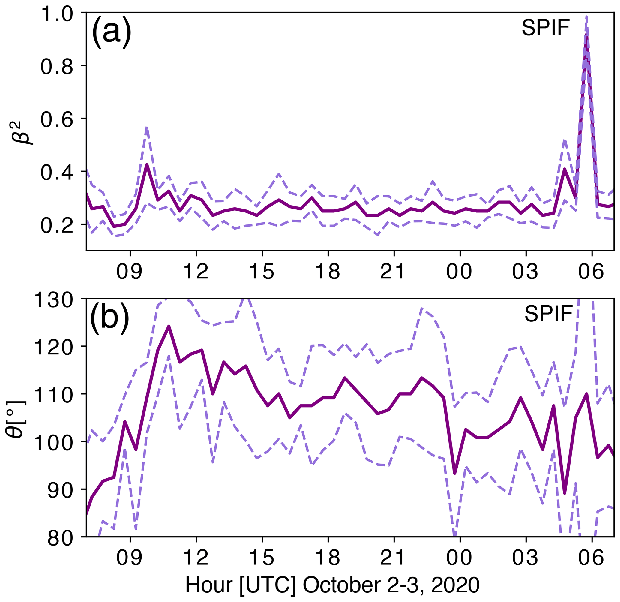
Figure B7 Back-azimuth analysis at the SPIF station. (a) Non-smoothed polarization degree β². The impulsive high-value polarization levels at ∼ 06:00 UTC on 3 October can be associated with anthropogenic noise sources, and they are also visible on different days. (b) Non-smoothed back-azimuth direction θ, averaged over 3–8 Hz. The mean is shown by a solid line and the standard deviation by the dashed lines.

Figure B8 The same plot as Fig. 2g but on a linear scale. Seismic power calculated in 2–10 Hz versus seismic power calculated in 10–45 Hz at the SPIF station. The seismic power peaks are marked in different colors.

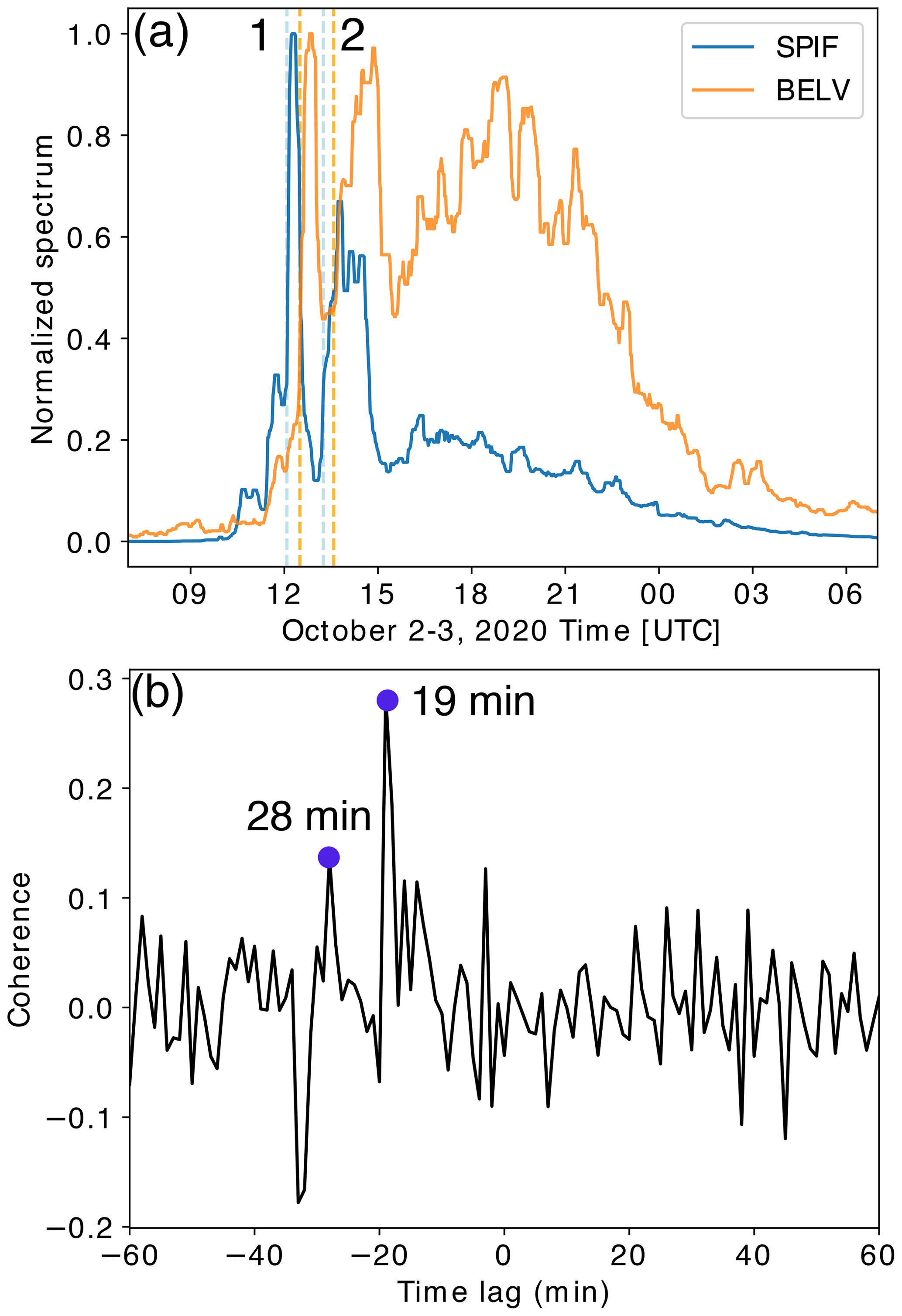
Figure B9 (a) Normalized seismic power recorded at the SPIF and the BELV stations smoothed over a 30 min moving time average. Arrivals times of peaks 1 and 2 are marked by dashed lines. (b) Normalized cross-correlation (coherence) between the normalized seismic power shown in (a).

Figure B10 Red: template located in the southern swarm. Black: examples of detected events by template matching. Seismograms show vertical ground velocity recorded at the station MVIF and are bandpass-filtered in the range 5–20 Hz.

Figure B11 Same as Fig. B10 but for a template located in the central swarm.

Figure B12 Same as Fig. B10 but for a template located in the northern swarm.