the Creative Commons Attribution 4.0 License.
the Creative Commons Attribution 4.0 License.
 | 11 Apr 2022
Rapid tsunami force prediction by mode-decomposition-based surrogate modeling
Kenta Tozato
Shinsuke Takase
Shuji Moriguchi
Kenjiro Terada
Yu Otake
Yo Fukutani
Kazuya Nojima
Masaaki Sakuraba
Hiromu Yokosu
This study presents a framework for rapid tsunami force predictions by the application of mode-decomposition-based surrogate modeling with 2D–3D coupled numerical simulations. A limited number of large-scale numerical analyses are performed for selection scenarios with variations in fault parameters to capture the distribution tendencies of the target risk indicators. Then, the proper orthogonal decomposition (POD) is applied to the analysis results to extract the principal modes that represent the temporal and spatial characteristics of tsunami forces. A surrogate model is then constructed by a linear combination of these modes, whose coefficients are defined as functions of the selected input parameters. A numerical example is presented to demonstrate the applicability of the proposed framework to one of the tsunami-affected areas during the Great East Japan Earthquake of 2011. Combining 2D and 3D versions of the stabilized finite element method, we carry out a series of high-precision numerical analyses with different input parameters to obtain a set of time history data of the tsunami forces acting on buildings and the inundation depths. POD is applied to the data set to construct the surrogate model that is capable of providing the predictions equivalent to the simulation results almost instantaneously. Based on the acceptable accuracy of the obtained results, it was confirmed that the proposed framework is a useful tool for evaluating time-series data of hydrodynamic force acting on buildings.
- Article
(34127 KB) - Full-text XML
-
Supplement
(15801 KB) - BibTeX
- EndNote


In order to estimate the potential damage due to a tsunami, predictions need to consider both the global aspect, such as the scale of the inundation areas, and also the local hydrodynamic forces acting on individual houses and each type of infrastructure. In fact, the potential effects of the tsunami force have been implemented in recent design standards (ASCE, 2017; Nakano, 2017). In addition, thanks to the extensive efforts made in recent years to develop numerical analysis techniques, maturity can be seen especially in the numerical analysis techniques applied to coastal engineering which provide highly accurate evaluations and predictions of tsunami forces (e.g., Qin et al., 2018; Xiong et al., 2019).
It is also extremely important for adequate disaster responses, such as evacuation actions, that information about the extent of damage can be quickly ascertained. In response to this demand, numerous studies have been made on instantaneous tsunami predictions. For example, NOAA (National Oceanic and Atmospheric Administration) constructed a real-time prediction system for tsunamis based on a long-term observation database (e.g., Titov et al., 2005; Tang et al., 2008, 2009; Wei et al., 2008). In addition, there have been many studies focused on the development of techniques for making real-time damage predictions based on numerical simulations. The studies can be classified into two types. In the first approach, the source and seismic waveform data are obtained from real-time observation systems, and then the tsunami propagation is calculated using input data estimated from the observed data. There have been a number of studies related to this approach: one on data-assimilation-based tsunami forecasting (Maeda et al., 2015), another on tsunami forecasting based on inversion for initial sea surface height (Tsushima et al., 2014), another to predict tsunami waveform using extreme learning machine (Mulia et al., 2016) and another using a real-time inundation simulation with supercomputers (e.g., Oishi et al., 2015; Musa et al., 2018). The second approach is based on the use of precomputed simulation data. Numerical simulations with multiple scenarios are carried out, and a tsunami database is numerically created to output prediction results immediately after an earthquake occurs. This approach is also widely accepted, and several studies have been reported. Among these is a study on making real-time predictions using source information and precomputed tsunami waveform and inundation databases (Gusman et al., 2014), another uses a combination of precomputed tsunami databases and the neural networks (Fauzi and Mizutani, 2019; Liu et al., 2021), and another features the surrogate modeling of numerical simulation results (e.g., Fukutani et al., 2019; Kotani et al., 2020).
The objective of this study is to evaluate the time series of the spatial distribution of tsunami forces acting on buildings in real time. Because a very high computational cost is required to evaluate the tsunami force over a wide area, it is generally difficult to perform such simulations in real time. Therefore, a surrogate-modeling-based prediction method is employed in this study. Surrogate modeling has been widely accepted for uncertainty quantification and probabilistic risk assessment, such as studies using response surface (e.g., Fukutani et al., 2019; Kotani et al., 2020), Gaussian process (e.g., Sarri et al., 2012; Salmanidou et al., 2017, 2021), polynomial chaos expansion (e.g., Denamiel et al., 2019; Giraldi et al., 2017; Sraj et al., 2017) and multifidelity sparse grids (e.g., de Baar and Roberts, 2017). These works demonstrate the potential of the surrogate-modeling-based approach, while the surrogate model considering spatiotemporal variation has not been well studied. Since this study considers time variation of spatial distribution of tsunami risk, a mode-decomposition technique is efficiently used to construct a surrogate model. Spatial modes and their equivalent principal components have been successfully utilized to construct surrogate models in the research fields of earthquake engineering and tsunami engineering. My Ha et al. (2008) proposed a surrogate model of a tsunami simulation by means of proper orthogonal decomposition (POD) for the purpose of reducing the dimensionality or, equivalently, the computational costs. In the fields of earthquake and structural engineering, there have been similar studies. Nojima et al. (2018) proposed to combine numerical simulations and a mode-decomposition technique that is based on the singular value decomposition for predicting the distribution of strong ground motions. Bamer and Bucher (2012) also used POD to construct a surrogate model to predict structural behavior using a nonlinear finite element analysis method. Since POD enables us to systematically extract the feature quantities of the temporal and spatial distributions of risk indicators, it is considered suitable for surrogate modeling for evaluating all kinds of disaster risks. Although some studies using mode-decomposition techniques have been reported in the research field of disaster science, the time–space surrogate modeling of tsunami force based on a high-precision 3D tsunami simulation has not been extensively studied.
The present study proposes a framework for rapid tsunami force predictions by the application of the POD-based surrogate modeling of numerical simulations. Only a limited number of large-scale numerical analyses are performed for a selection of scenarios with various fault parameters to capture the distribution tendencies of the target risk indicators. After 2D shallow water simulations are performed, the results are used as input data for 3D flow simulations to evaluate the time histories of forces acting on buildings. Then, POD is applied to the evaluation results to extract the principal modes that represent the temporal and spatial characteristics of the forces caused by a target tsunami. A surrogate model can then be constructed by a linear combination of spatial modes whose coefficients are determined by means of the regression analysis and interpolation techniques. To demonstrate the applicability of the proposed framework, one of the tsunami-affected areas during the Great East Japan Earthquake of 2011 is targeted. Using the 2D simulation and the results obtained for different input parameters, we carry out a series of 3D numerical analyses to obtain a set of time history data of the spatial distributions of tsunami force and then construct a surrogate model capable of predicting the time variations of the spatial distributions of tsunami forces almost instantaneously. A surrogate model of the inundation depth is also constructed and compared with that of tsunami force.
The structure of this paper is as follows. Section 2 explains the flow and specific procedures of the proposed framework. In Sect. 3, the proposed framework is applied to a target city to construct the surrogate model that enables rapid predictions of tsunami forces equivalent to the 3D tsunami run-up simulations.
This section describes the flow and methodologies of the proposed framework. In the framework proposed in this study, we carry out a series of 2D–3D coupled tsunami analyses with selected sets of fault parameters corresponding to expected scenarios beforehand to obtain a limited number of scenario-specific simulation results. Then, the principal spatial modes of tsunami forces are extracted from the precomputed simulation data to construct the surrogate model for the rapid tsunami force prediction. It is to be noted that the coefficients of the modes are interpolated in the parameter space so as to be functions of fault parameters. Thus, because this study stands on the assumption that the fault parameters are given when an actual tsunami event occurs, the tsunami force prediction is made immediately using the constructed surrogate model. Figure 1 shows the flowchart of the proposed method. Each part of the proposed method, such as tsunami analyses, mode decomposition and surrogate modeling, is explained in detail in the following subsections.
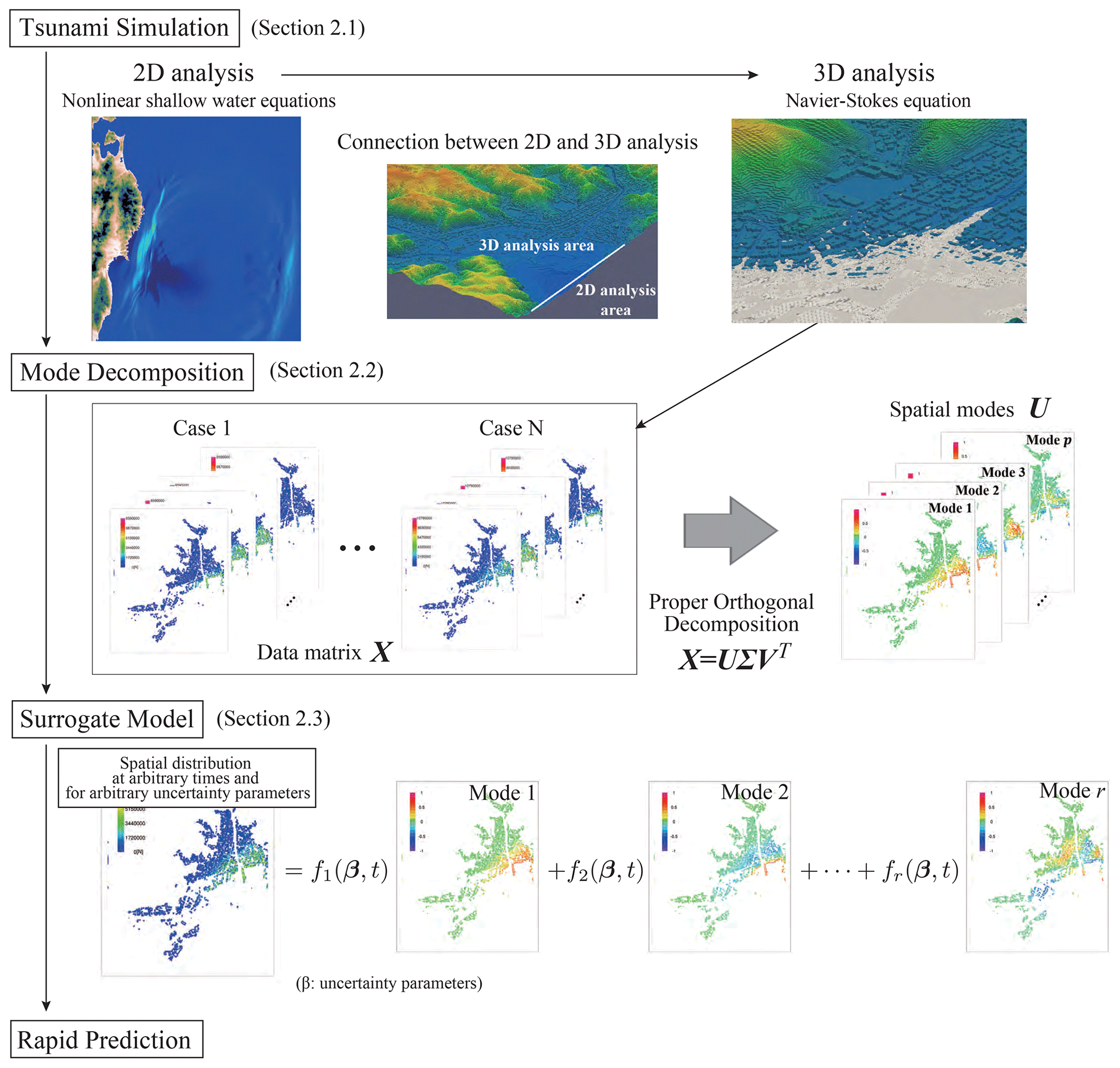
Figure 1Flowchart of the rapid tsunami force prediction by the mode-decomposition-based surrogate model.
2.1 2D–3D coupled tsunami analyses
To collect the data necessary for the surrogate modeling explained in the previous section, a set of two sequential numerical analyses are carried out for each case with a selected set of fault parameters. A 2D tsunami analysis is first carried out to obtain the information about the tsunami wave caused by the offshore fault. Then, the time histories of the tsunami height and flow velocity on the specified boundary of the target urban area are extracted for use as input data for a 3D tsunami run-up simulation. A 3D numerical analysis is performed to elaborately evaluate the spatial and temporal distributions of risk indicators within the target area. Since the risk indicators in this study include not only the inundation depth but also the force acting on buildings, the 3D calculation requires a high-fidelity numerical analysis. In this section, only the governing equations for 2D and 3D tsunami simulations are outlined. For the details of their connection, Takase et al. (2016) can be referenced.
To numerically analyze tsunami wave propagation over a wide area, 2D shallow water simulations are commonly performed. TUNAMI-N2 (Tohoku University's Numerical Analysis Model for Investigation of Near-field Tsunamis No. 2) (Imamura, 1995; Goto et al., 1997), one of the most well-known simulation codes, is based on the concept of the shallow water theory. In this study, we employ the TUNAMI-N2 to represent wave propagation in the offshore area. The following formats of continuity and nonlinear long wave equations are solved in the 2D analysis:
where M and N are the flow rates in the x and y directions, η is the water level, D is the total water depth, g is gravitational acceleration, and n is the Manning roughness coefficient. To evaluate the force acting on buildings, we employ the following set of 3D Navier–Stokes and continuity equations in the analysis domain Ωns∈R3:
where ρ is the mass density, u is the velocity vector, σ is the stress tensor, and f is the body force vector. Also, assuming a Newtonian fluid, the stress is calculated as
where p is the pressure, μ is the coefficient of viscosity, and ε(u) is the velocity gradient tensor defined as
To solve the governing equations of the 3D analysis, the stabilized finite element method (SFEM) is employed in this study. Details of the method are explained in the appendix(see Appendix A).
2.2 Mode decomposition
Proper orthogonal decomposition (POD) (Liang et al., 2002) is well known as a technique to extract the principal direction along which the variance of the collected data is maximized. In other words, POD is capable of grasping the characteristics of data and expressing data in a lower dimension. When applying POD to data, we prepare a matrix storing the data arranged in accordance with a certain rule (hereafter, referred to as the “data matrix”). When n data are obtained for scenario case i, they are stored into a column vector denoted by xi, which has n components. Here, n is the number of evaluation points for risk indicators, namely the tsunami force and inundation depth in this study. When the scenario ranges from 1 to N, the data matrix can be defined as
Here, a vertical line is added to each column vector to indicate that the component alignment follows the specified rule. In POD, the data matrix is generally constructed with the mean subtraction, but in this study, the procedure was not applied because the accuracy of the constructed surrogate model with subtraction was almost the same as the one without subtraction. In the case of time–space mode decomposition, a data matrix is defined by storing the data for each time in the column direction. The covariance matrix of the data matrix is defined as
The eigenvectors are the principal directions, and the corresponding eigenvalue represents the variance in each principal direction. Also, larger eigenvalues have more major contributions to the data.
Let λj be the jth eigenvalue of C and uj be the jth eigenvector . Since each eigenvalue corresponds to the variance in the corresponding principal direction or mode, those with small eigenvalues have almost no significant values and provide little meaningful information, and therefore they can be omitted in the sequel. To omit unnecessary modes, the contribution rate is generally introduced as an indicator to compare the magnitude of each eigenvalue with others. Specifically, the contribution rate dj of a particular mode j is defined as a percentage of each eigenvalue against the sum of all eigenvalues as
When this rate is arranged in descending order, the threshold for the omission is determined according to the profile of its decreasing curve. It should be noted that the information about the omitted mode is lost and is a source of error.
Also, based on the theory of singular value decomposition, data matrix X can be expressed as
where U is a matrix lining up the eigenvector uj of C in the column direction, and V is the matrix lining up the eigenvector vj and matrix in the column direction. Also, Σ is the matrix having the square roots of eigenvalues in the diagonal components, which are referred to as singular values. Here, p is the number of singular values that must be greater than zero. Equation (11) can be substituted for C and C′ to have their eigenvalue decomposition as
It follows that C and C′ have common non-zero eigenvalues, each of which is equal to the squared singular value of X, and that U and V in Eq. (11) correspond to the eigenvectors of C and C′, respectively.
Additionally, from the relational expression of the singular value decomposition, data vector xi for case i is expressed as the linear combination of the eigenvectors of the covariance matrix as
where vij are components of V with i and j indicating row and column numbers, respectively. Here, the modes are arranged in accordance with the descending order of the corresponding eigenvalues, and αik is the coefficient of the kth mode associated with the ith case. Once modes to be omitted are determined according to the magnitude relationships of the contribution rates, amongst others, the number of modes r used to approximate the data is determined so that the equation above yields the following reduced-order expression:
where is expected to be a close approximation of the original data xi for the ith case. In this manner, data for a certain case can be expressed as a linear combination of major modes expressing the fundamental features. Remember that each of these selected modes corresponds to the eigenvector of the covariance matrix whose associated eigenvalue is relatively larger then others. As acknowledged above, errors may occur in Eq. (15) due to the truncation or mode omission.
2.3 Construction of the surrogate model
Once the reduced-order expressions of all the data vectors are obtained, a surrogate model can be obtained straightforwardly. We begin with identifying the relationship between the coefficient for each mode and the set of input parameters β, each of which corresponds to a selected scenario or case. That is, coefficients αik are approximated as functions of parameters β by interpolation or regression, which are denoted by fk(β) . Then, the surrogate model can be expressed in the following equation whose independent variables are input parameters β:
In this study, fk(β) is determined by the interpolation with radial basis function (RBF) interpolation (Buhmann, 1990) which is regarded as a Gaussian process (GP) regression. The GP regression is applicable even if the parameters are not distributed in equidistant intervals and even if some defects and high nonlinearity are present in the data.
RBF interpolation for fk(β) can be expressed by the following equation:
where βi contains the set of parameters for case i, wi is the weight, and are RBFs. Here, γ is the parameter controlling the smoothness of the function. Because fk(β), which is a coefficient of mode k shown in Eq. (17), is individually interpolated, wi and γ have different values for each mode. By substituting the set of actual input parameters in Eq. (17), we obtain the following simultaneous equations to determine the set of weights wi:
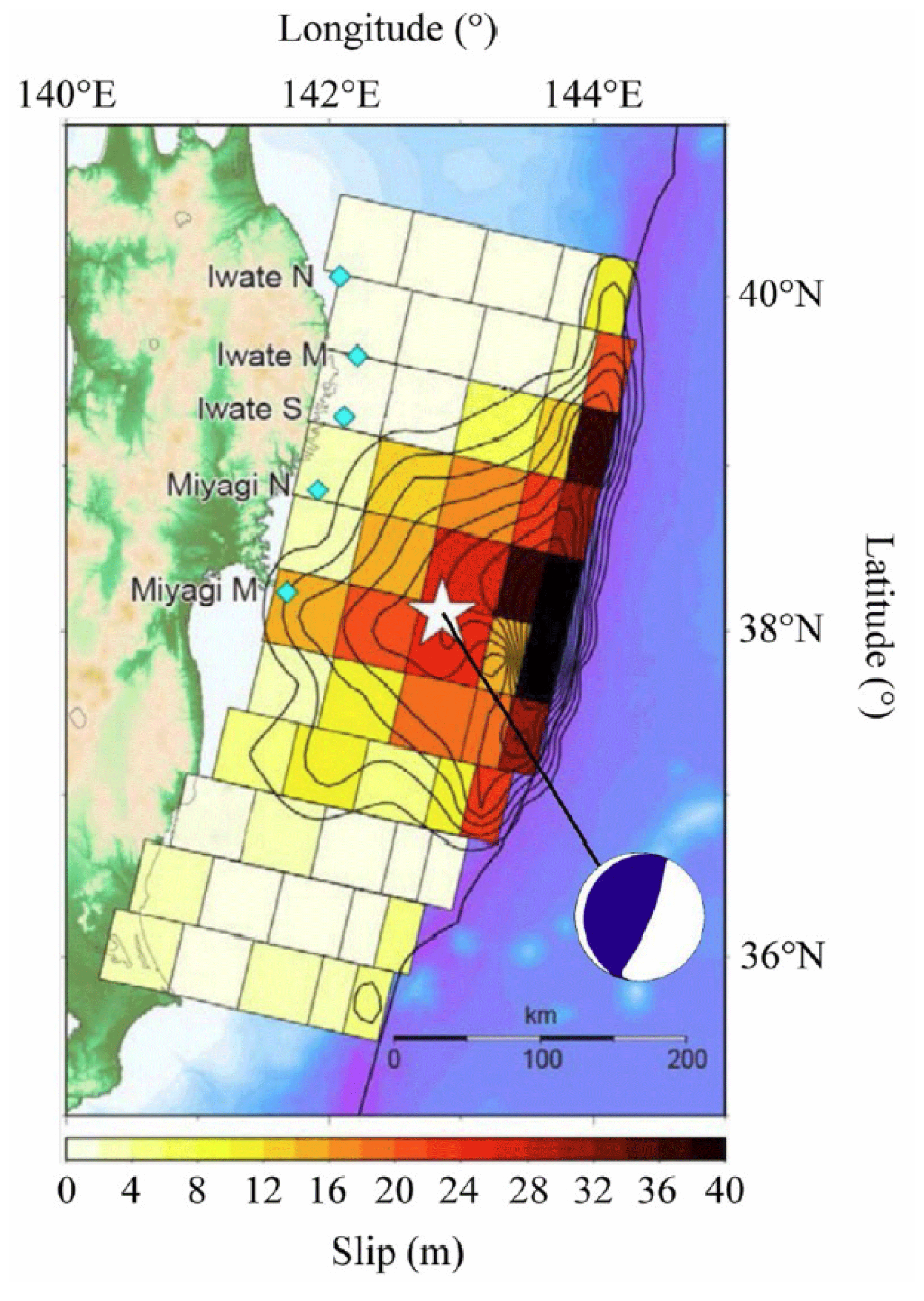
Figure 2Fujii–Satake model ver. 8.0 (adapted from Kotani et al., 2020).
In this study, ridge regression (Hoerl and Kennard, 1970) is used to compute weights for Eq. (18). The weights are obtained by solving the following optimization problem:
where λ is the regularization parameter, αk is the vector of coefficients for the kth mode, wk is the vector of weights for the kth mode, and Φ is the coefficient matrix in Eq. (18). By introducing the ridge regression, it is possible to prevent the overfitting problem. Since the accuracy of the interpolation depends on the regularization parameter λ and the smoothness parameter γ of the RBF interpolation, these values are determined by the application of a certain cross-validation technique (Stone, 1974). In this study, four-folded cross-validation is applied to determine the parameters γ and λ, and the Bayesian optimization (Močkus, 1975) is used to efficiently search for the optimal values γ and λ in the parameter space.
In this section, the proposed method is applied to tsunamis that have occurred. The simulation and the construction of the surrogate model are based on the tsunami induced by the 2011 earthquake that occurred off the Pacific coast of Tohoku.
3.1 Tsunami simulation
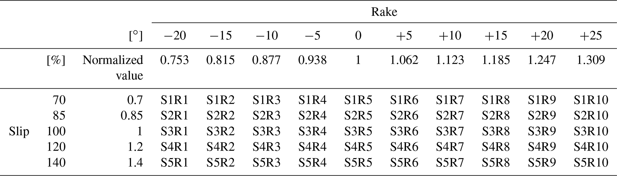
In this study, as previously mentioned, the calculation was performed in two steps, including a numerical analysis based on the 2011 earthquake that occurred off the Pacific coast of Tohoku using 2D analysis over a wide area and 3D run-up analysis for the target region. To construct a surrogate model that considers uncertainty, it is first necessary to decide what uncertainty should be considered. Next, we considered the dominant factors from the occurrence of the tsunami to its run-up. For example, the epicenter position and magnitude are factors that need to be considered during the earthquake. During tsunami propagation, the fault model that controls the initial waveform of the tsunami and the submarine topography data need to be included. In this study, the 2011 earthquake that occurred off the Pacific coast of Tohoku was used as a basis. That is, the relevant factors in the process of the earthquake itself can be found in the accomplishments of research conducted up to this point. In specific terms, in our study, we used a fault model (Fujii–Satake model ver. 8.0) (Satake et al., 2013) composed of the 55 small faults shown in Fig. 2. By considering uncertainty in terms of the two parameters of slip and rake in Fig. 3, which are thought to have a deep relationship with the characteristics of fault stagger, we conducted a numerical analysis of multiple scenarios using different values of these parameters. The cases that were analyzed and the names of the cases are shown in Table 2. For the slip of each small fault, there were five patterns from 0.7 to 1.4, and for the rake, there were 10 patterns with −20 and changes in the angle, making a total of 50 cases.

Figure 3Illustration of the fault parameters (adapted from Kotani et al., 2020).
3.1.1 Wide-area 2D tsunami analysis
To obtain the information about the tsunami wave usable for the 3D analysis, a tsunami analysis is carried out utilizing the 2D shallow water flow model. First, a wide-area 2D analysis was performed to obtain time history data for the tsunami height and flow velocity observed within the bay of the target region. Regarding the initial waveform of the tsunami, Okada (1992) was employed. The fluctuation vertical component close to the seabed was calculated based on the fault model, and the initial water level fluctuation was determined. Additionally, an analysis mesh was created with intervals of 2430, 810, 270 and 90 m, and nesting was performed to subdivide this mesh in relation to the target based on the tsunami wave source. An image of this nesting is shown in Fig. 4. To confirm the reasonableness of the obtained 2D analysis, we compared the results to the actual measured values of the fluctuation in the tsunami water level of the 2011 earthquake that occurred off the Pacific coast of Tohoku. As a point of comparison, we used the GPS wave meter observation data of the NOWPHAS (2022) provided by the Ports and Harbours Bureau, Ministry of Land, Infrastructure, Transport and Tourism. The observation positions were offshore to the north of Iwate Prefecture (No. 1), offshore to the center of Iwate Prefecture (No. 2), offshore to the south of Iwate Prefecture (No. 3), offshore to the north of Miyagi Prefecture (No. 4) and offshore to the center of Miyagi Prefecture (No. 5), and a comparison of these is shown in Fig. 5. The result is that the actual measured values were sufficiently reproduced, and a 3D tsunami analysis was performed using these results as input values.
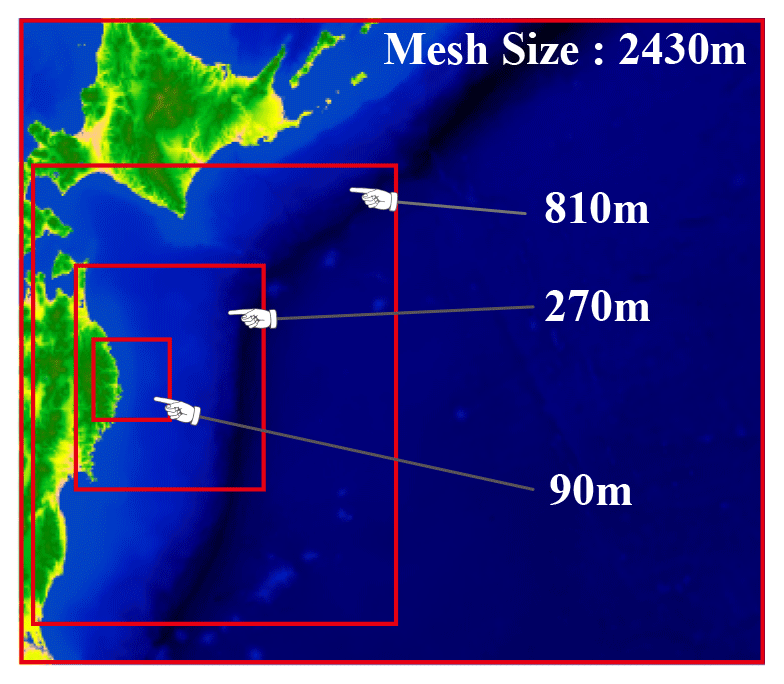
Figure 4Nested analysis regions (adapted from Kotani et al., 2020).

Figure 5Comparison of tsunami height between observational data and simulation results (borrowed from Kotani et al., 2020).
3.1.2 Connecting the 2D and 3D analyses
Using the results of the 2D tsunami analysis over a wide area as the input conditions, a 3D tsunami analysis was performed to represent the tsunami run-up in the target region. As mentioned before, the method used in Takase et al. (2016) was employed to couple the 2D and 3D models together. An image of the location of the 2D–3D boundary is shown in Fig. 6. The time-series data of the wave height and flow velocity obtained from the 2D wide-area analysis are stored and transferred to the 3D numerical analysis by linear interpolation in space. Also, since the time interval in the 2D calculation differs from that in the 3D one, the 2D results are linearly interpolated in the time domain, and the interpolated values are given to the 3D analysis as input data. The reason why the 2D–3D boundary is placed at the mouth of the bay is that the boundary can be defined by a straight line.
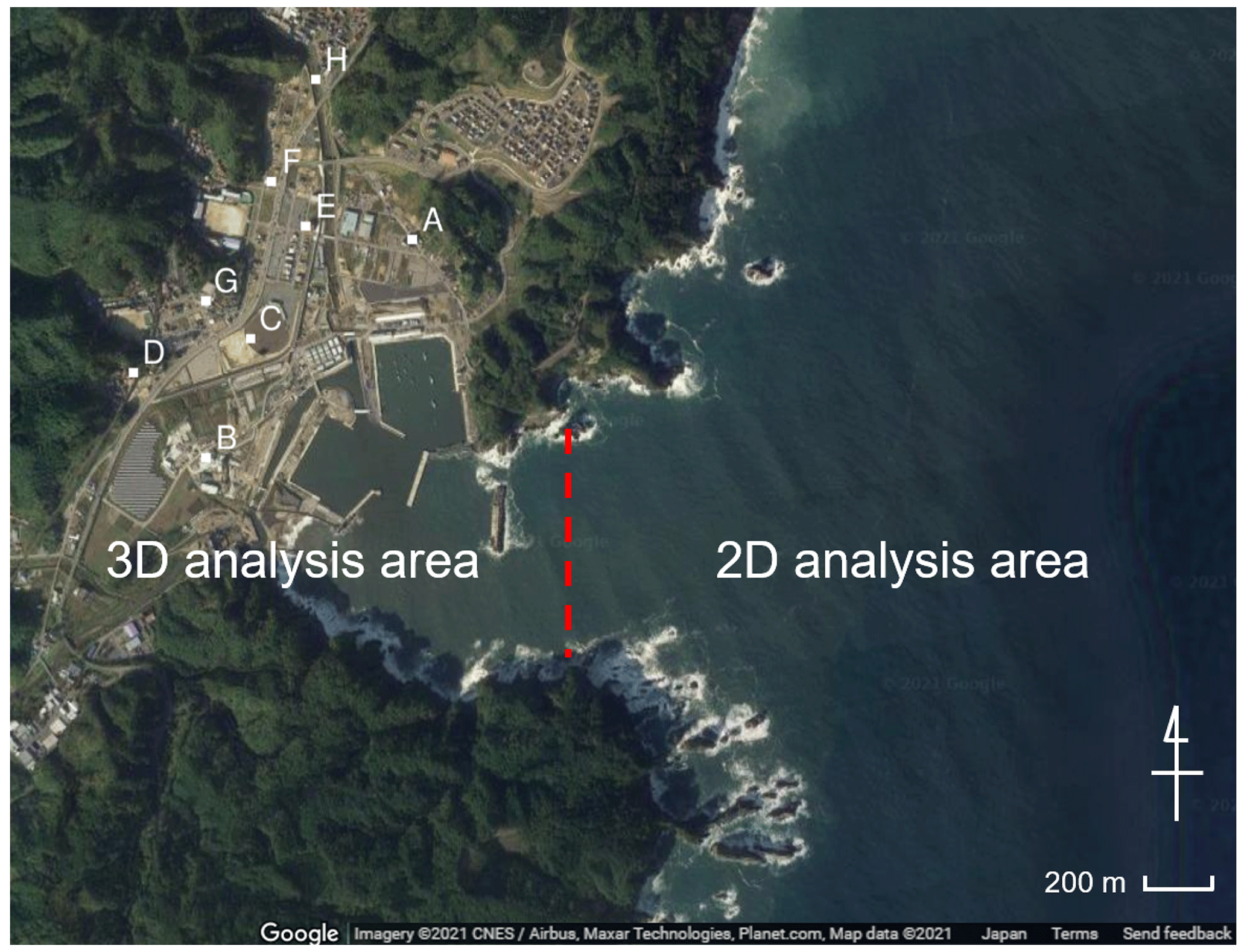
Figure 6Boundary between the 2D analysis and 3D analysis areas. Points A to H are used to compare the inundation depths between observational data and simulation results (© Google Maps).
3.1.3 3D run-up analyses
Tsunami run-up was represented by the 3D analysis using SFEM on the 2145 m×2600 m field shown in Fig. 8. Images of the FE mesh used in this analysis are described in Fig. 7. A fine mesh with a minimum mesh size of 1.5 m is used around buildings, and a coarse mesh with a maximum mesh size of 10 m is used for mountainous areas. The non-slip boundary condition is used on building surfaces and ground surfaces. Figure 8 shows snapshots of the tsunami run-up obtained in the 3D simulation. A very complex 3D flow that cannot be represented in 2D simulations is seen in the simulated results. As mentioned in Sect. 3.1, the calculation condition of Case S3R5 corresponds to the real tsunami induced by the 2011 earthquake that occurred off the Pacific coast of Tohoku. Therefore, we checked the accuracy of the simulated result obtained in Case S3R5 by comparing it with survey results. Data of the maximum inundation heights are provided by the 2011 Tohoku Earthquake Tsunami Joint Survey Group (2012). Figure 9 indicates a comparison between simulated maximum inundation heights and survey data. The evaluation points are shown in Fig. 6. The comparison shows that the simulated inundation heights near the coastline (points A, B, C and E) represent well the real inundation heights, while there are big gaps at other points. The reason for these big gaps is that the buildings are assumed to be rigid bodies, and the buildings are not washed away in the 3D analysis. Although most of buildings were washed away due to the tsunami, buildings suppress tsunami run-up in the analysis. While this suggests it is better to consider the effect of washing away buildings, modeling this effect is difficult. Furthermore, the main objective of this study is to construct a surrogate model of tsunami force and discuss its performance. We therefore conclude that the simulated results in this study roughly express the real tsunami.
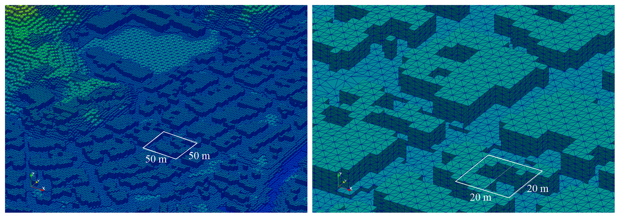

Figure 8Snapshots of tsunami run-up obtained in 3D analysis. The white-colored area represents the inundation area.
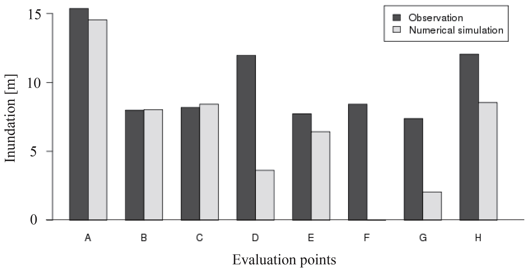
Figure 9Comparison of inundation heights between observational data and simulation results (observation data are provided by the 2011 Tohoku Earthquake Tsunami Joint Survey Group, 2012).
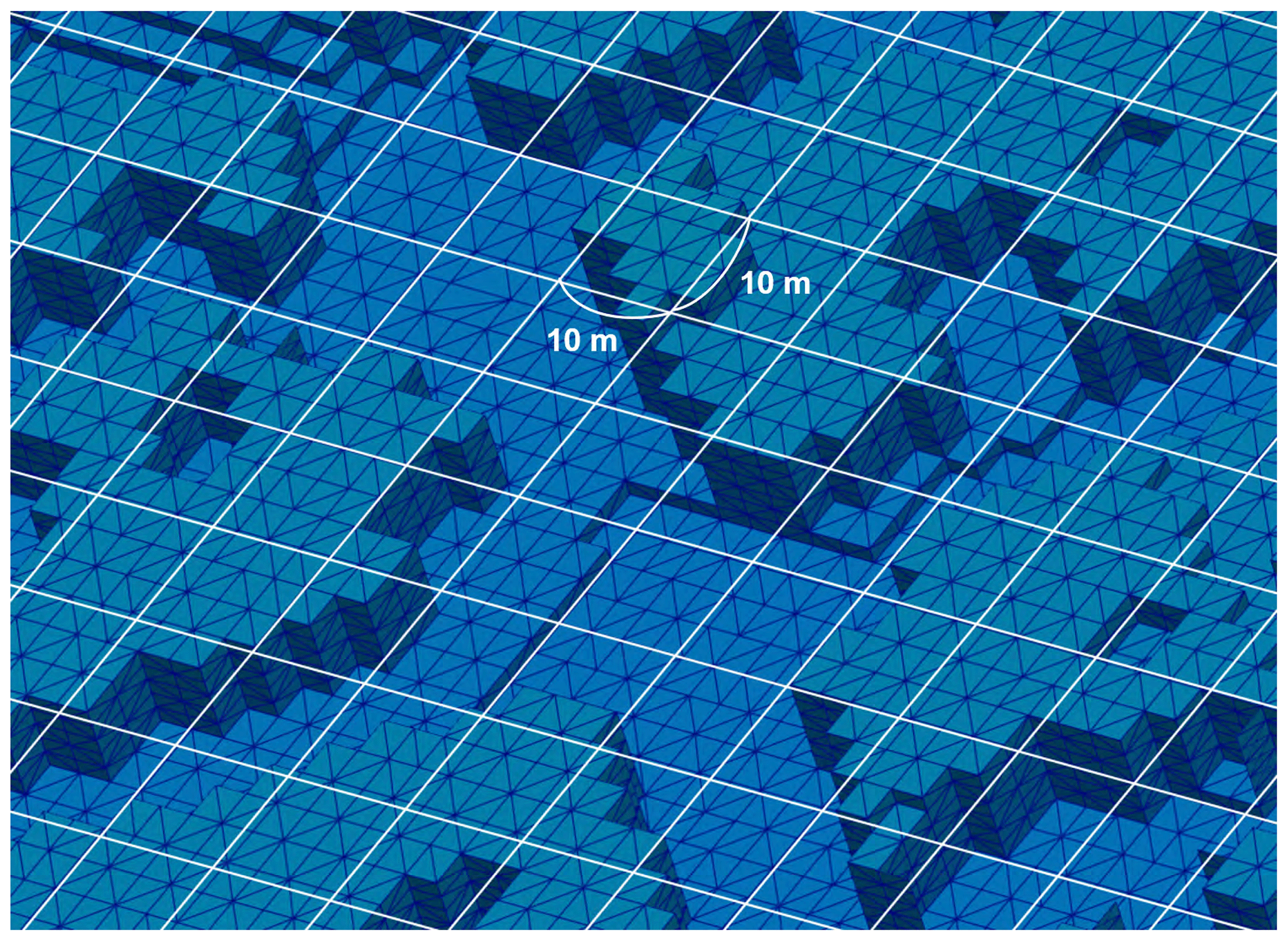
In order to construct a surrogate model of tsunami force, we can use the hydrodynamic force acting on buildings calculated in the 3D simulation. It is, however, difficult to quantify pointwise tsunami force because the force is strongly affected by the direction of building surfaces. To avoid this problem, we consider a 2D mesh with a grid size of 10 m for evaluating the tsunami force. The tsunami force is evaluated by averaging in each of these sub-domains but not for each building in this study. An image of the mesh is shown in Fig. 10. The force acting on the building surface is integrated in each mesh and quantified as a scalar value. The spatial distribution of the tsunami force was obtained in this manner.
3.2 Application of proper orthogonal decomposition
3.2.1 Definition of the target risk indicators and data matrix
In this study, the tsunami force acting on the buildings and the inundation depth are used as the target risk indicators, and the values integrated or averaged in the 10 m mesh are used as the mean values. As the field is 2145 m×2600 m, the number of evaluated points is . The impact force is calculated by using the pressure and the surface affected by the pressure in a 10 m square. Additionally, 20 s is used for the time interval for the data, and 150 steps of data are used in accordance with the time for the tsunami run-up. In this application example, in addition to the two input parameters, time is introduced as another parameter because when predicting damage rapidly, it is necessary to evaluate the state of time-related developments in addition to spatial distribution.
Proper orthogonal decomposition is applied to construct a surrogate model for the results of 40 of the 50 cases shown in Table 1, excluding the 10 cases for which the rake is . The reason that these 10 cases are not used for surrogate model construction is that their associated data are later used to verify the reasonableness of the created surrogate model. Additionally, as 40 cases secured a sufficient number of analysis cases for the two variables in this study, verification is not performed, but it is desirable to assess how many cases are required when constructing the surrogate model.
Next, the data matrix is defined. First, the time-series data for a particular scenario can be defined as follows as matrix Xi.
Here, is a vector containing the spatial distribution of a risk indicator in relation to time. Specifically, in this study, the tsunami force and inundation depth at each grid point are selected for the indicators, and their time-series data are stored in separate data matrices, each of which consists of the data vectors at each time. Additionally, as a specific parameter, Ui expresses slip in relation to scenario (slip), and λi expresses rake in relation to scenario i. Additionally, m expresses the maximum number of output steps in the numerical analysis, and in the example in this study, this is m=150. Data matrix X is defined as follows, as laid out in the column direction.
In this study, because time–space mode decomposition is performed, the data for each calculation case and each time are aligned in the column direction of the data matrix. The previously described proper orthogonal decomposition was carried out for this data matrix. By applying proper orthogonal decomposition to this matrix, it is possible to extract a common temporal mode for data including time. Temporal effects are expressed by the coefficients of the modes, and it is possible to construct a surrogate model including the time direction.
3.2.2 Extracted spatial modes and construction of a surrogate model
Here, we show the results of applying proper orthogonal decomposition in relation to impact force and inundation data.
First, in relation to the extracted spatial mode, the impact force and water depth for the first mode to the third mode are shown in Fig. 11.
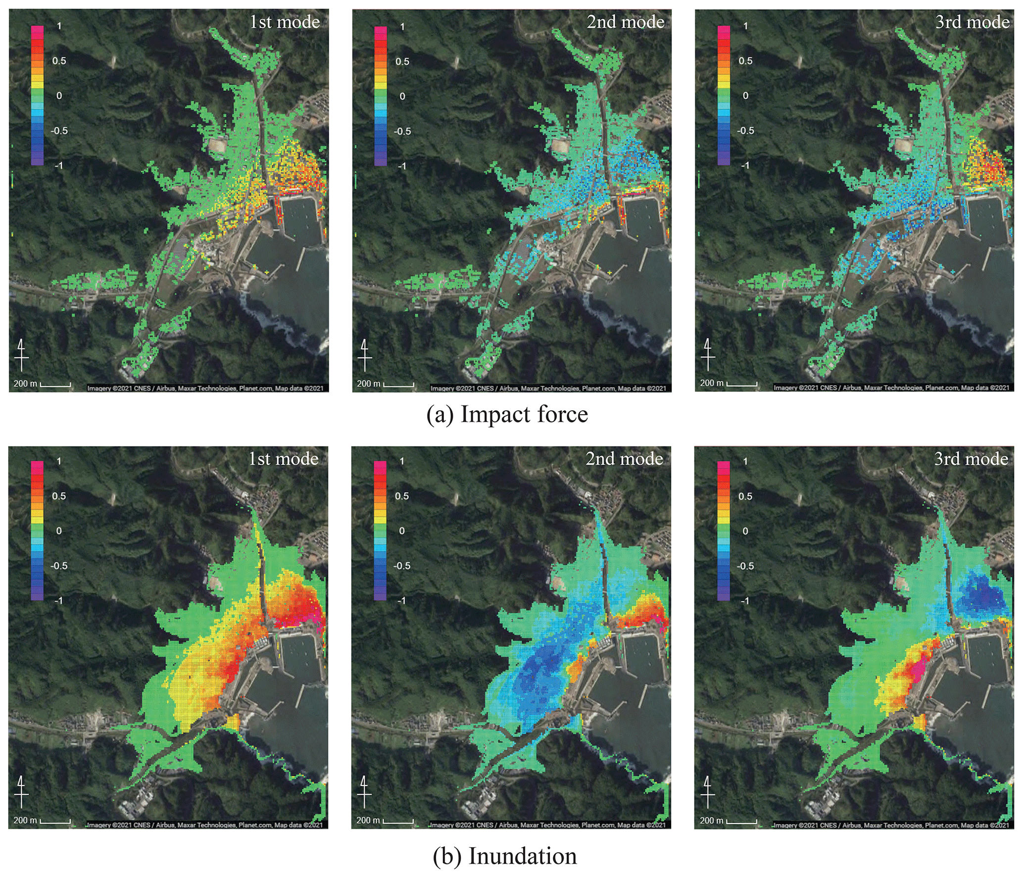
Figure 11Spatial modes of (a) impact force and (b) inundation depth extracted by POD (© Google Maps).
The values in Fig. 11 show the normalized ones for each mode. From these figures, it can be confirmed that the impact force distribution and inundation depth distribution both have roughly the same spatial distribution characteristics. If we examine the characteristics in more detail, in the case of the first mode, we can see the tendency for the coastal side to be most strongly impacted. Naturally, since the points close to the coast are most affected by the tsunami, this is a mode that best expresses this kind of impact. The second mode expresses opposite tendencies for the section close to the coast and the section behind it, and the third mode expresses opposite tendencies for the eastern and western coastal areas. In general, the lower-order modes have higher contributions with respect to the original data, while the higher-order modes represent local effects, and their contributions are relatively small.
The contribution rates of the impact force and water depth are shown in Fig. 12. The contribution in the first mode is extremely high for both impact force and inundation depth. In this study, as an indicator of the number of modes, the error and the contribution rate were investigated. In this example, for the 10 cases of data kept aside as verification data, the root mean squared error for the results obtained from the numerical analysis and the results obtained from the surrogate model for each mode are calculated. The error of case ei is calculated using the following equation.
Here, n is the number of evaluation points, and m is the number of time step. Additionally, Xi is time-series data of numerical simulation results for the ith case, and values are results obtained from a surrogate model with r modes. The relations between the number of modes and the error for each risk index are shown in Fig. 13. From Fig. 13, it can be seen that the error decreases as the number of modes used in the surrogate model increases, and as the number of modes increases, the error rates decrease, thus gradually converging. In this study, 20 modes are used to construct the surrogate models because the error has been sufficiently reduced.
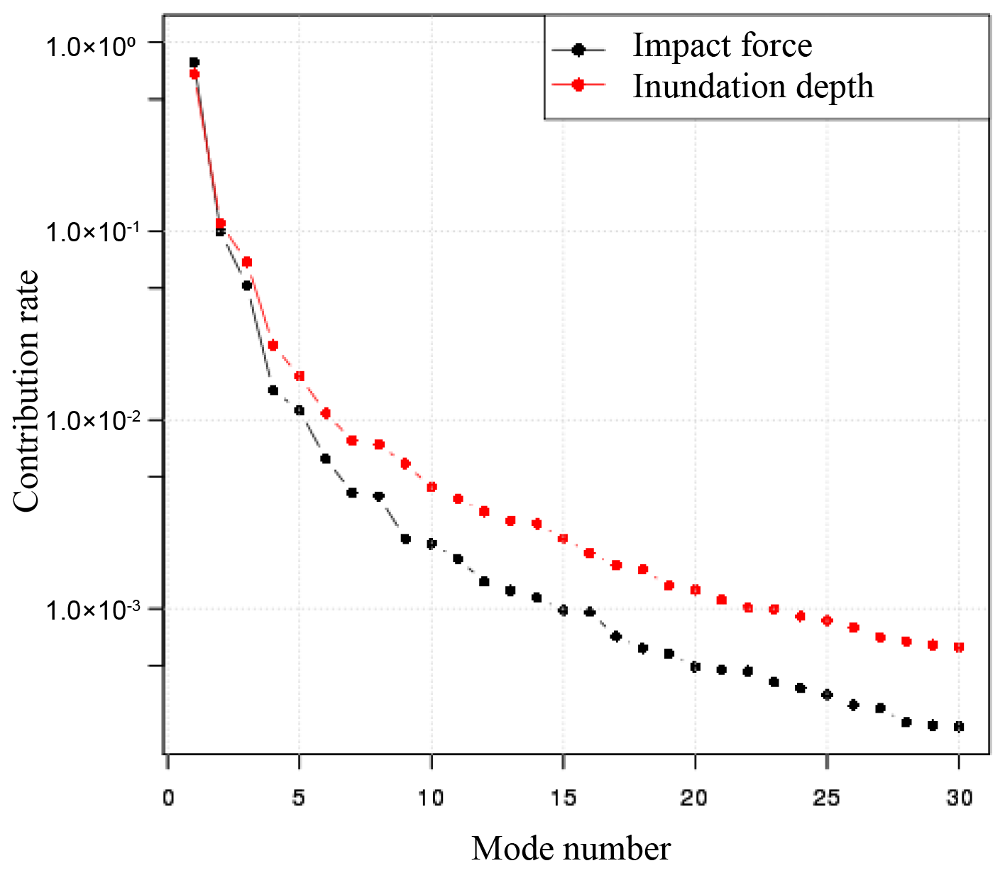
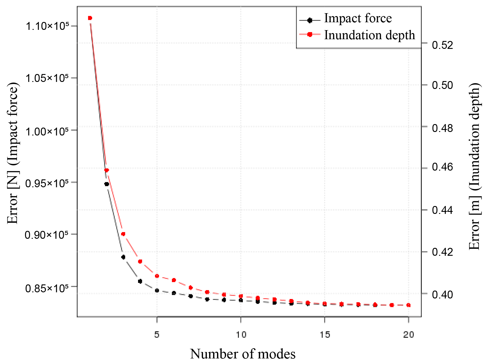
Figure 13The root mean squared error for the results obtained from the numerical analysis and those of the surrogate models for each mode.
Next, by interpolating the proper orthogonal decomposition coefficient as a parameter function, the surrogate models are created. As shown in Eq. (21), as the data matrix contains the slip U, rake λ and time t, which are parameters for numerical analysis in the column direction, the proper orthogonal decomposition coefficient is also expressed as a function of slip, rake and time. In specific terms, this coefficient can be expressed as as in the following equation.
3.2.3 Reconstructing the numerical simulation results
Here, we compare the results obtained from the numerical analysis and the results from reconstructing the original data using the constructed surrogate models. First, when comparing the time-series data, several evaluation points are set. In this study, the 10 points shown in Fig. 14 are set as evaluation points. Next, for the average case scenario S3R5, a comparison of the numerical analysis results and the results when reconstructing data using the surrogate models are shown. Snapshots of the impact force and water depth are shown in Fig. 15, and the time-series data for each physical quantity at points 2 and 3 in Fig. 14 are shown in Fig. 16. Although only the time-series data obtained at the three points are shown in the figure, the same tendency is confirmed at other points. The black line indicates the results obtained from the actual numerical analysis, and the red line shows the results from reconstructing data using the surrogate models. Using the time-series data of the impact forces shown in Fig. 16a, it is possible to calculate the impulse acting on the buildings. The impulse can be obtained by integrating the force in time. Values of the impulse calculated by the numerical simulation and calculated by the surrogate models for the 10 evaluation points are shown in Fig. 17.
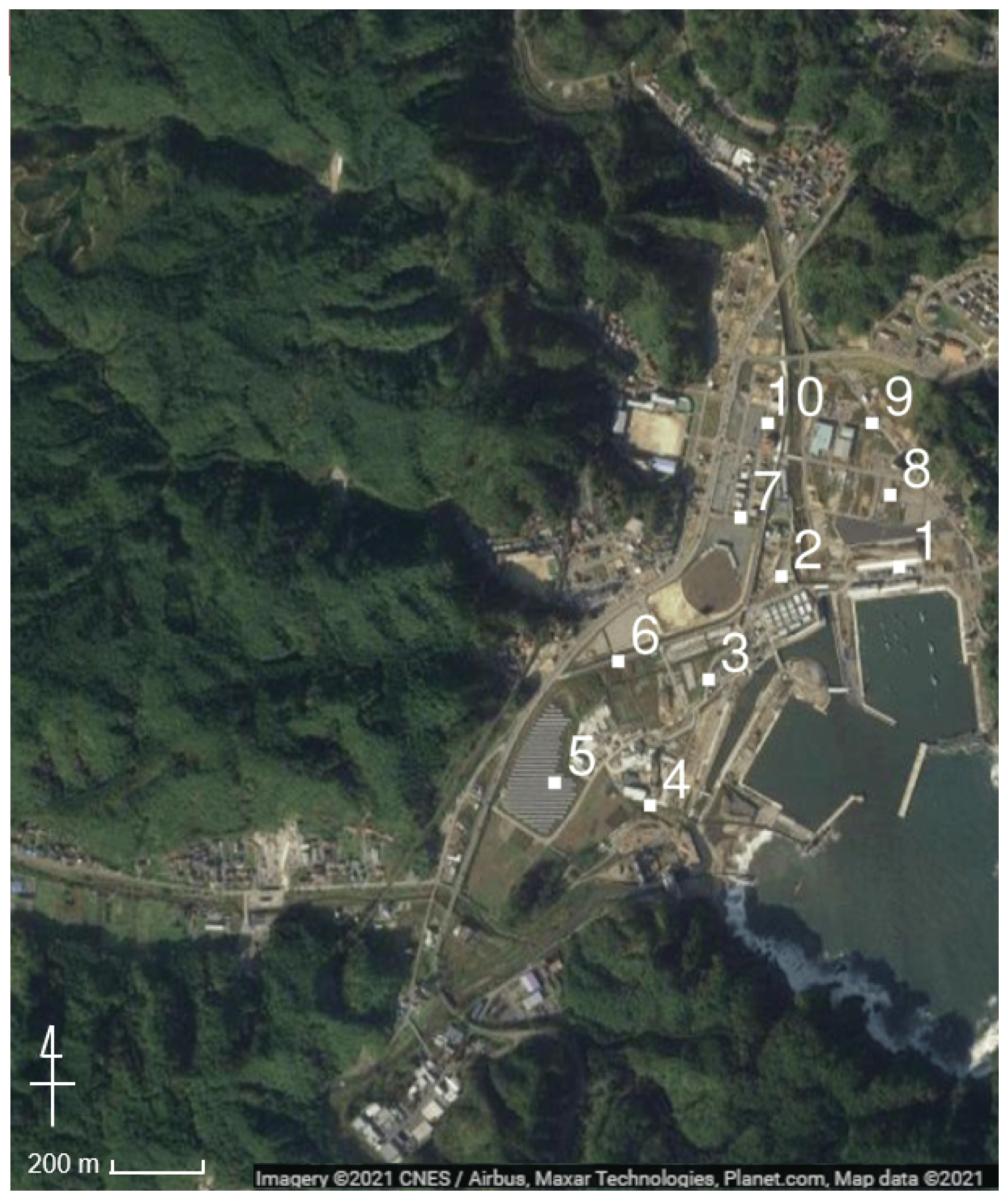
Figure 14Evaluation points for comparing results obtained from numerical simulation and those of the surrogate models (© Google Maps).
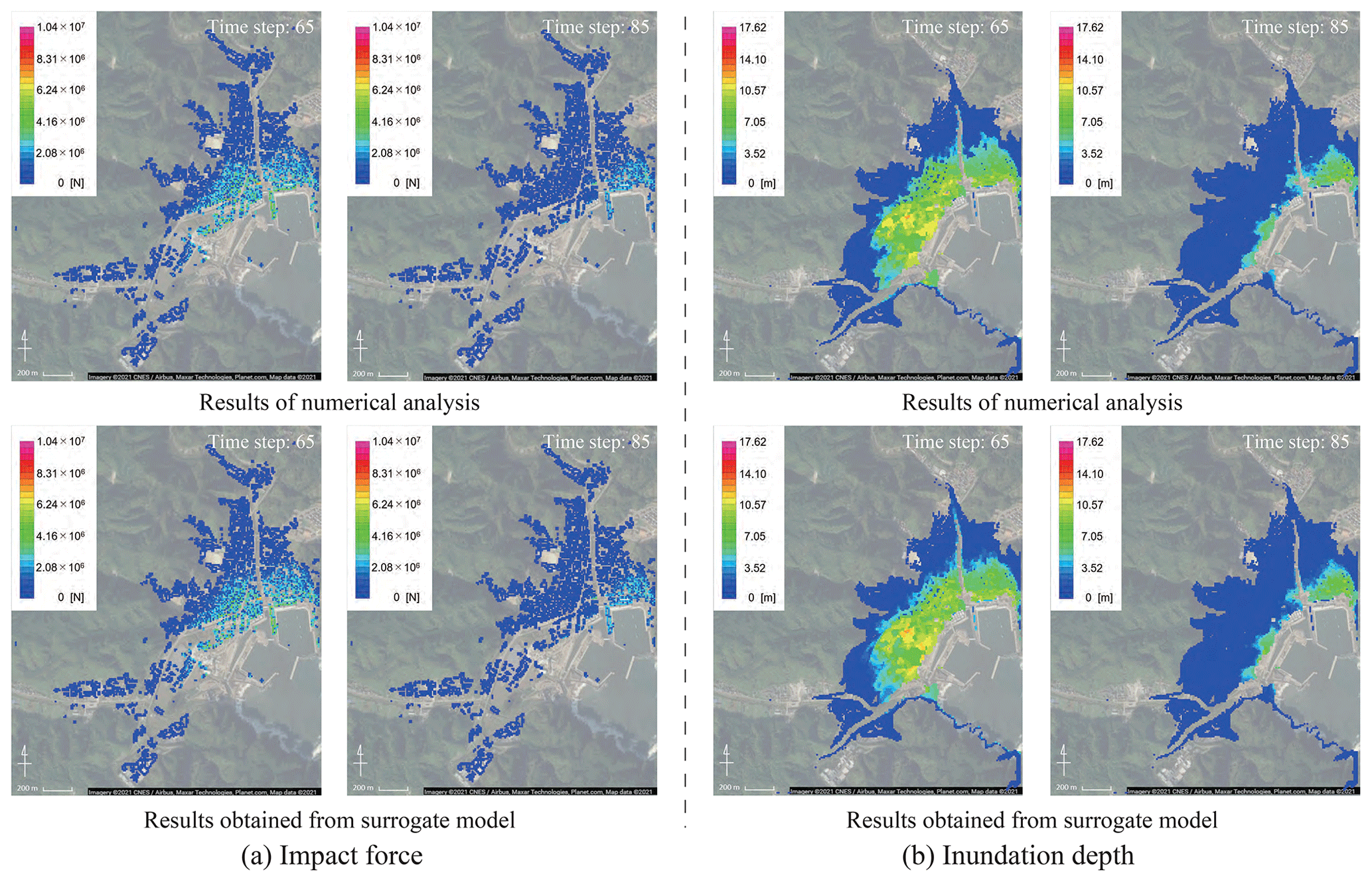
Figure 15Snapshots of the results obtained from numerical analysis and those reconstructed by using spatial modes (© Google Maps).
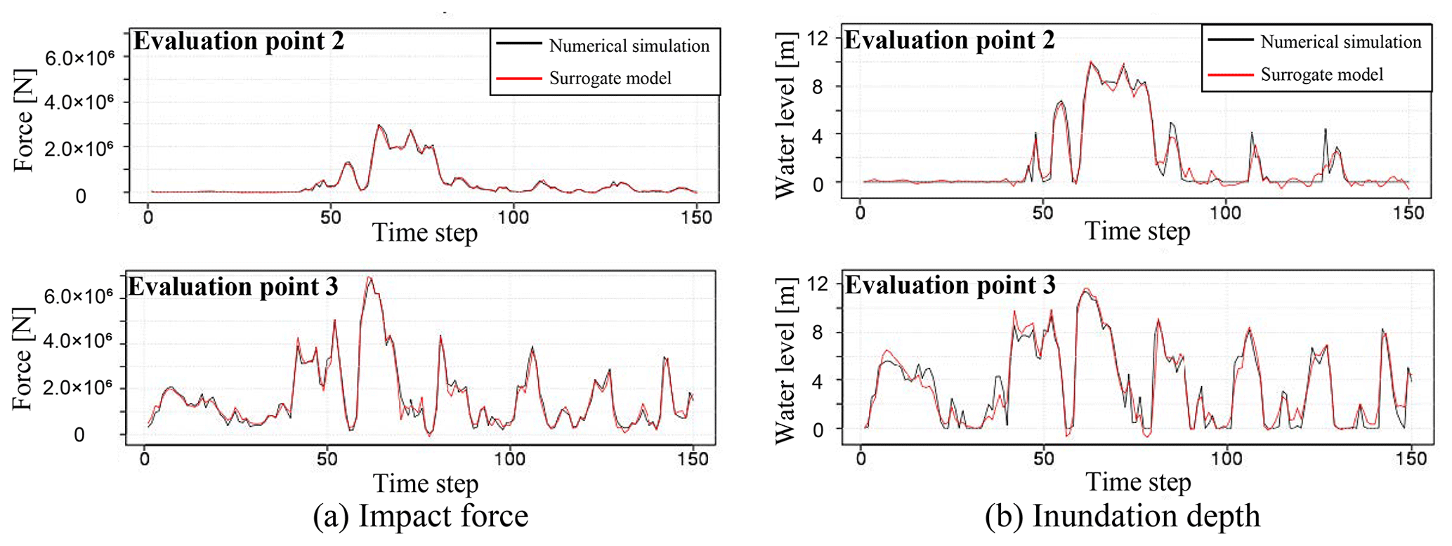
Figure 16Comparison of time-series data obtained from numerical analysis and those reconstructed by using spatial modes.

Figure 17Comparison of impulses calculated from the results of numerical analysis and the results reconstructed by using spatial modes.
Based on these results, it can be summarized that whereas errors partially occur based on the impact of mode reduction, in general, the original data are being reproduced, and it is possible to express the data as a linear combination of modes. It should also be noted that there are different tendencies between spatial distributions of tsunami force and those of inundation depth. For instance, at time step 65, high values are locally seen in the inundation depth, while that tendency is not seen in the result of tsunami force. This indicates that it is difficult to predict damage to buildings based on only inundation depth, and information on tsunami force is also required for an accurate damage prediction.
3.2.4 Validation of the surrogate models
By comparing data that were not used for the construction of the surrogate models, it is possible to investigate whether the surrogate models could reproduce the numerical analysis results. A comparison of the results obtained from the numerical analysis and the surrogate models for the two scenarios of S2R3 and S5R7 is shown in Figs. 18–20. As in the previous section, for each physical quantity, a comparison by snapshots and time-series data at evaluation points 2 and 3 is shown.
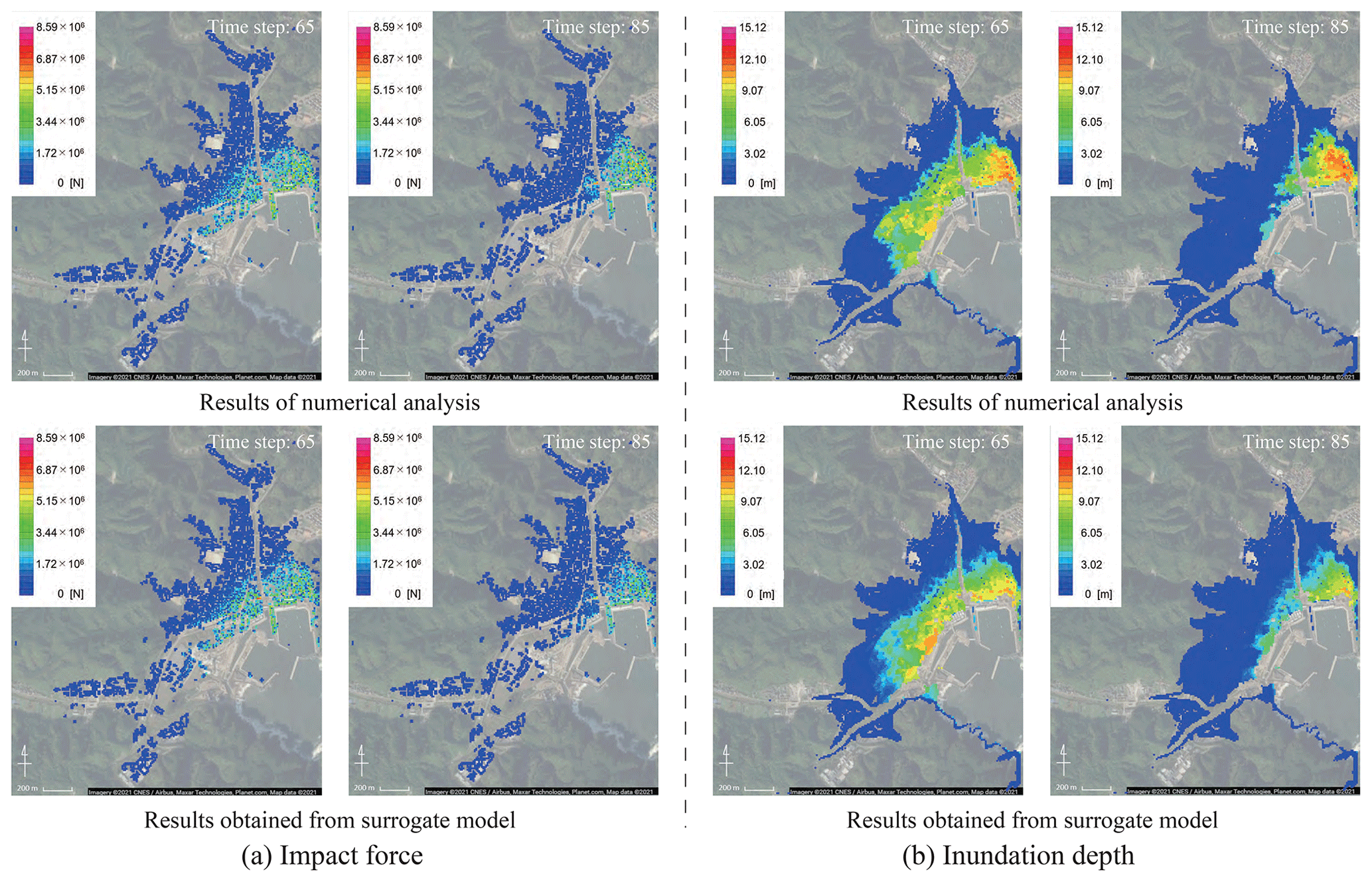
Figure 18Snapshots of the results obtained from numerical analysis and those obtained from the surrogate models (S2R3) (© Google Maps).
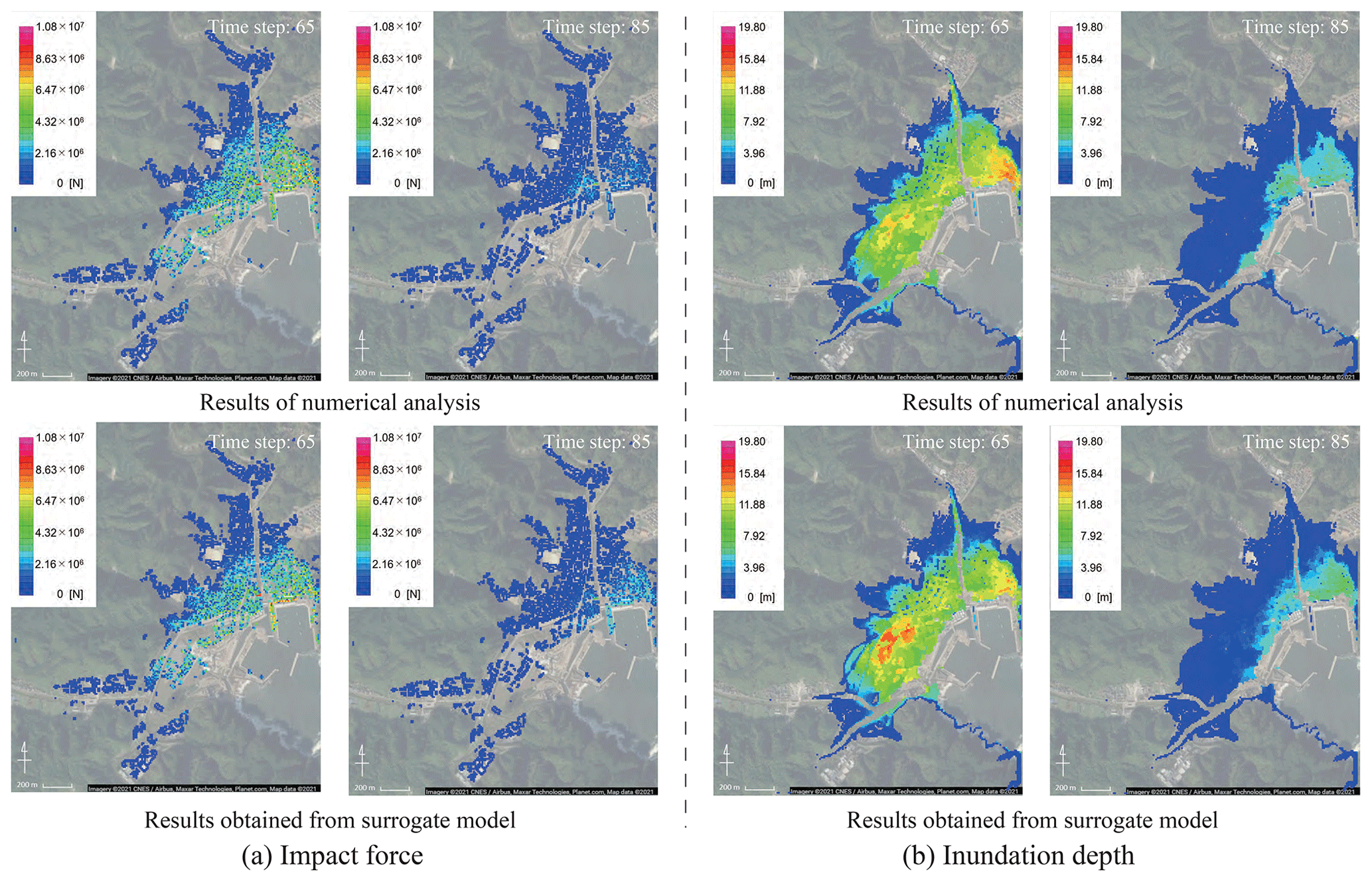
Figure 19Snapshots of the results obtained from numerical analysis and those obtained from the surrogate models (S5R7) (© Google Maps).
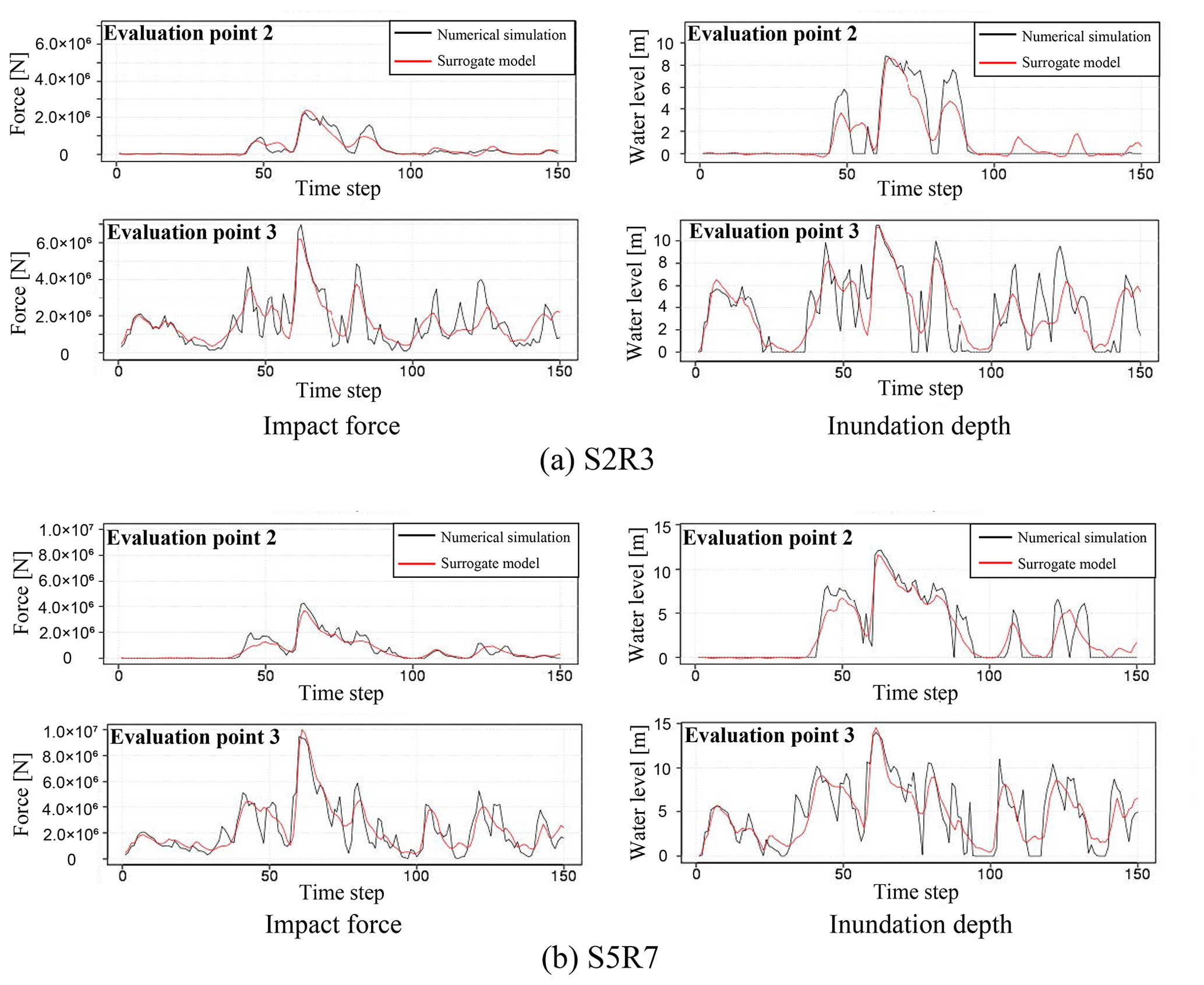
Figure 20Comparison of time-series data obtained from the numerical analysis and the surrogate models.
Here, it is confirmed that it is possible to represent the simulation results using arbitrary parameters with the surrogate models. However, as shown in Figs. 18 and 19, it should be noted that the surrogate models do not fully represent the local spatial distribution. More advanced mode-decomposition techniques, such as the sparse modeling, are needed to improve the accuracy.
Next, the root mean squared error (RMSE) for the time-series data at all points is calculated for each of the physical quantities by using Eq. (22). The relative errors in the mean value and the maximum value are presented in Table 2. Here, “mean value” is a root mean square of the corresponding quantity.
Table 2Error between the results of the numerical analysis and the results obtained from the surrogate models.
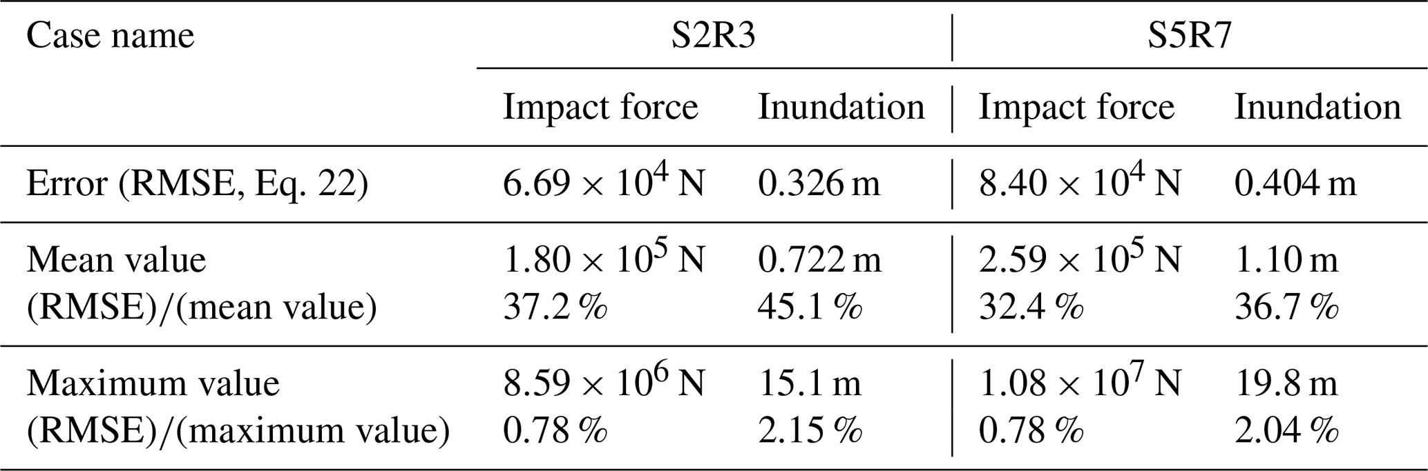
With regard to Table 2, the relative error of the mean value of time-series data for a specific scenario was 37.2 % for the impact force data and 45.1 % for the water depth data in S2R3 and 32.4 % for the impact force data and 36.7 % for the water depth data in S5R7. It is acknowledged that these are very high values. This large error comes from inadequate representation of local peaks and the phase shift. In addition, because the time-series data include a large amount of data that would not be affected by a tsunami, such as data from mountainous areas, the data include many values equal or close to zero: this would result in extremely small mean values. That is, it is likely that the large error rate value in calculations is because of the small mean values. Note that the relative error to the maximum value of time-series data for a specific scenario is 0.78 % for the impact force data and 2.15 % for the water depth data for S2R3 and 0.78 % for the impact force data and 2.04 % for the water depth data in the case of S5R7. In these cases, the error rate is low compared to the maximum value. In other words, because the error in Table 2 is sufficiently small compared to the maximum value, the overall distribution and the general shape of the time-series data can be roughly captured by the surrogate models.
Next, as in the previous section, the impulse is calculated using the time-series data of the impact forces, and a comparison of the impulse calculated from the numerical analysis results and the results obtained from the surrogate model for the 10 evaluation points is shown in Fig. 21.
Figure 21 shows that the surrogate model can adequately represent the impulse calculated from the numerical simulation results. Since the impulse can visualize the risk that cannot be seen by the maximum impact force alone, it can be fully utilized for the tsunami risk assessment for buildings in the target area.
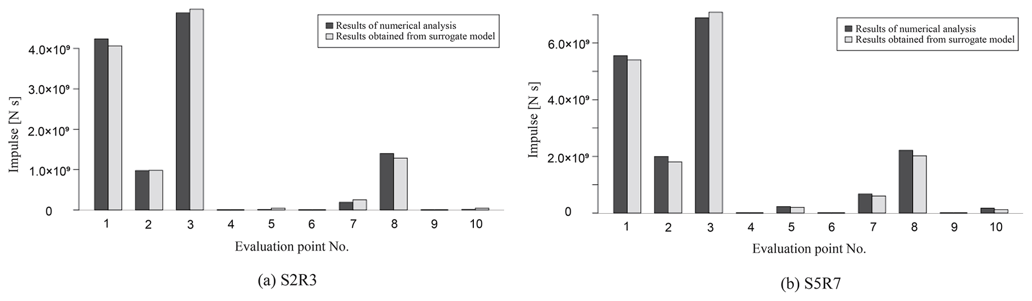
Figure 21Comparison of impulses calculated from the results of numerical analysis and those obtained from the surrogate models (a, S2R3; b, S5R7).
Furthermore, the surrogate model has distinct advantages in terms of calculation costs. A total of 4 h were required to complete the numerical analysis of one case when using a 16 parallel computing Intel™ Xeon™ CPU E5-2667 v4 (3.20 GHz) for the 2D calculation. In the case of the 3D analysis, using an 8 node 544 core Intel™ Xeon™ Phi KNL (1.4 GHz), the calculation time was approximately 96 h. Once the model was constructed, however, the calculation using the surrogate model took only a few seconds, and because it was possible to calculate the spatiotemporal distribution of the physical quantity using arbitrary parameters, it would be possible to apply the surrogate model using the spatial modes for rapid damage prediction.
This study presents the framework for predicting time-series data of tsunami force based on the results of a high-precision numerical analysis at a low calculation cost. By performing proper orthogonal decomposition in relation to the numerical analysis results while considering uncertainty, we could extract spatial modes and express the spatial distribution of the risk indicators as a linear distribution of the modes. Additionally, by expressing the coefficients as functions of analysis parameters and time in the surrogate models, it was possible to calculate the distribution at extremely low calculation costs for certain cases for which no numerical analysis has been performed. In this study, surrogate models of the impact force and inundation depth of a tsunami running up to a target area were constructed, and it was shown that the results of the numerical analysis could be roughly represented. It is also shown that the impulse calculated from the time-series data of the tsunami force obtained from the surrogate model can sufficiently represent the numerical simulation results. These results indicate that the surrogate models can be efficiently utilized for tsunami risk assessments.
In this study, for tsunami events, only the two fault parameters of slip and rake were considered as uncertainties. However, as many uncertainties are at play in an actual tsunami event, it would be possible to integrate these parameters and perform a numerical analysis and, in the same manner, create a surrogate model that incorporates a larger range of uncertainties in more detail. Nevertheless, when increasing the types of input parameters, as the number of scenarios that need to be considered becomes immense, it is pertinent to use efficient methods for parameter sampling such as Latin hypercubes (McKay, 1979). Furthermore, it is very important to evaluate in advance the extent to which these uncertainty parameters will fluctuate. In the surrogate model created in this study, a sufficient evaluation was performed with interpolation (within the scope of the parameters for which numerical analysis was conducted). However, with extrapolation (outside the scope of the parameters for which numerical analysis was conducted), the possibility of reduced accuracy is high, so it is necessary to evaluate in advance the extent to which the uncertainty parameters fluctuate and set scenarios that allow for this range of fluctuation.
While the mechanism shown in this paper was designed for use with tsunamis, it has potential for use in the rapid prediction of various disasters. Since numerical simulations of disasters typically involve high computational costs, it is important to consider uncertainty in advance and perform a numerical analysis before creating a surrogate model. That is, the rapid prediction developed by the surrogate model proposed in this work can be used as a tool to gauge the extent of disasters.
With regard to Eqs. (4) and (5), we apply the stabilized finite element method equipped with the streamline upwind Petrov–Galerkin (SUPG) and pressure-stabilizing Petrov–Galerkin (PSPG) (SUPG/PSPG) method (Tezduyar, 1991) to obtain the following finite element equation.
Here, Ωns∈ℝ3 is the analysis domain, nel is the number of elements, uh and ph are the finite element approximations for velocity and pressure, respectively, and wh and qh are the approximations of the weight functions for the equations of motion and continuity, respectively. Also, the fourth involves the SUPG term for stabilizing the advection process and the PSPG term for avoiding pressure oscillation. In addition, the fifth term has the shock-capturing term (Aliabadi and Tezduyar, 2000) for avoiding numerical instability on free surfaces, and , and are all stabilization parameters.
In this study, the phase-field approach is employed to capture the complex geometries of free surfaces, such as breaking waves and flow around buildings. In this approach, the locations of free surfaces can be determined by solving the Allen–Cahn advection equation (Chiu and Lin, 2011; Takada et al., 2013), which was modified to the storage format as
where the phase-field function ϕ takes 1.0 or 0.0 to identify liquid (water) and gas (air) phases, and an intermediate value represents the free surface. Here, ε is the mobility, and δ is the representative width of the free surface. According to the phase-field function, the fluid density ρ and viscosity coefficient μ for each element were evaluated as
where subscripts l and g indicate the quantities of the liquid and gas, respectively.
In this study, we also apply the stabilized finite element method with the SUPG method to the Allen–Cahn equation above so that the resulting finite element equations are given as
where ϕh and are finite element approximations for the phase-field function ϕ and its weight function, respectively. Here, τϕ is the stabilization parameter defined as
where he is the characteristic length of an element.
Source code and details of the tsunami simulation were sourced from Kotani et al. (2020). Outputs of the simulations are available in the Zenodo open-access repository at https://doi.org/10.5281/zenodo.6394294 (Tozato, 2022).
The supplement related to this article is available online at: https://doi.org/10.5194/nhess-22-1267-2022-supplement.
KTo contributed to analyzing the simulated data and constructing surrogate models. ST, KN and MS provided the simulated data of 2D and 3D analyses. SM, KTe, YO and YF contributed to proposing the framework and supervising the surrogate modeling. KTo, SM and KTe prepared the manuscript. HY led the discussion with practical viewpoints. All authors read and approved the final paper.
The contact author has declared that neither they nor their co-authors have any competing interests.
Publisher's note: Copernicus Publications remains neutral with regard to jurisdictional claims in published maps and institutional affiliations.
The authors would like to gratefully acknowledge the support made through Chubu Electric Power (Public Research Concerning Nuclear Power).
This paper was edited by Paolo Tarolli and reviewed by four anonymous referees.
Aliabadi, S. and Tezduyar, T. E.: Stabilized-finite-element/interface-capturing technique for parallel computation of unsteady flows with interfaces, Comput. Method. Appl. M., 190, 243–261, https://doi.org/10.1016/S0045-7825(00)00200-0, 2000. a
American Society of Civil Engineers: ASCE standard “Minimum design loads for buildings and other structures” (ASCE/SEI 7-16), https://doi.org/10.1061/9780784414248, 2017. a
Bamer, F. and Bucher, C.: Application of the proper orthogonal decomposition for linear and nonlinear structures under transient excitations, Acta Mech., 223, 2549–2563, https://doi.org/10.1007/s00707-012-0726-9, 2012. a
Buhmann, M. D.: Multivariate cardinal interpolation with radial-basis functions, Constr. Approx., 6, 225–255, https://doi.org/10.1007/BF01890410, 1990. a
Chiu, P. H. and Lin, Y. T.: A conservative phase field method for solving incompressible two-phase flows, J. Comput. Phys., 230, 185–204, https://doi.org/10.1016/j.jcp.2010.09.021, 2011. a
de Baar, J. H. S. and Roberts, S. G.: Multifidelity Sparse-Grid-Based Uncertainty Quantification for the Hokkaido Nansei-oki Tsunami, Pure Appl. Geophys., 174, 3107–3121, https://doi.org/10.1007/s00024-017-1606-y, 2017. a
Denamiel, C., Šepić, J., Huan, X., Bolzer, C., and Vilibić, I.: Stochastic Surrogate Model for Meteotsunami Early Warning System in the Eastern Adriatic Sea, J. Geophys. Res.-Oceans, 124, 8485–8499, https://doi.org/10.1029/2019JC015574, 2019. a
Fauzi, A. and Mizutani, N.: Machine learning algorithms for real-time tsunami inundation forecasting: A case study in Nankai region, Pure Appl. Geophys., 177, 1437–1450, https://doi.org/10.1007/s00024-019-02364-4, 2019. a
Fukutani, Y., Moriguchi, S., Terada, K., Kotani, T., Otake, Y., and Kitano, T.: Tsunami hazard and risk assessment for multiple buildings by considering the spatial correlation of wave height using copulas, Nat. Hazards Earth Syst. Sci., 19, 2619–2634, https://doi.org/10.5194/nhess-19-2619-2019, 2019. a, b
Giraldi, L., Maître, O. P. L., Mandli, K. T., Dawson, C. N., Hoteit, I., and Knio, O. M.: Bayesian inference of earthquake parameters from buoy data using a polynomial chaos-based surrogate, Computat. Geosci., 21, 683–699, https://doi.org/10.1007/s10596-017-9646-z, 2017. a
Goto, C., Ogawa, Y., Shuto, N., and Imamura, F.: Numerical method of tsunami simulation with the leap-frog scheme, in: IUGG/IOC TIME Project, IOC Manual and Guides, UNESCO, Paris, 35, 1–126, http://www.vliz.be/imisdocs/publications/269372.pdf (last access: 29 March 2022), 1997. a
Gusman, A. R., Tanioka, Y., MacInnes, B. T., and Tsushima, H.: A methodology for near-field tsunami inundation forecasting: Application to the 2011 Tohoku tsunami, J. Geophys. Res.-Sol. Ea., 119, 8186–8206, https://doi.org/10.1002/2014JB010958, 2014. a
Hoerl, A. E. and Kennard, R. W.: Ridge regression: Biased estimation for nonorthogonal problems, Technometrics, 12, 55–67, https://doi.org/10.1080/00401706.1970.10488634, 1970. a
Imamura, F.: Review of tsunami simulation with a finite difference method, in: Long-Wave Runup Models, edited by: Yeh, H., Liu, P., and Synolakis, C., World Scientific Publishing, Hackensack, NJ, 25–42, https://doi.org/10.1142/9789814530330, 1995. a
Kotani, T., Tozato, K., Takase, S., Moriguchi, S., Terada, K., Fukutani, Y., Otake, Y., Nojima, K., Sakuraba, M., and Choe, Y.: Probabilistic tsunami hazard assessment with simulation-based response surfaces, Coast. Eng., 160, 103719, https://doi.org/10.1016/j.coastaleng.2020.103719, 2020. a, b, c, d, e, f, g
Liang, Y. C., Lee, H. P., Lim, S. P., Lin, W. Z., Lee, K. H., and Wu, C. G.: Proper orthogonal decomposition and its applications-Part I: theory, J. Sound Vib., 252, 527–544, https://doi.org/10.1006/jsvi.2001.4041, 2002. a
Liu, C. M., Rim, D., Baraldi, R., and LeVeque, R. J.: Comparison of Machine Learning Approaches for Tsunami Forecasting from Sparse Observations, Pure Appl. Geophys., 178, 5129–5153, https://doi.org/10.1007/s00024-021-02841-9, 2021. a
Maeda, T., Obara, K., Shinohara, M., Kanazawa, T., and Uehira, K.: Successive estimation of a tsunami wavefield without earthquake source data: A data assimilation approach toward real-time tsunami forecasting, Geophys. Res. Lett., 42, 7923–7932, https://doi.org/10.1002/2015GL065588, 2015. a
McKay, M. D., Beckman, R. J., and Conover, W. J.: A comparison of three methods for selecting values of input variables in the analysis of output from a computer code, Technometrics, 21, 239–245, https://doi.org/10.2307/1268522, 1979. a
Močkus, J.: On bayesian methods for seeking the extremum, in: Optimization Techniques IFIP Technical Conference Novosibirsk, Springer, Berlin, Heidelberg, 400–404, https://doi.org/10.1007/3-540-07165-2_55, 1975. a
Mulia, I. E., Asano, T., and Nagayama, A.: Real-time forecasting of near-field tsunami waveforms at coastal areas using a regularized extreme learning machine, Coast. Eng., 109, 1–8, https://doi.org/10.1016/j.coastaleng.2015.11.010, 2016. a
Musa, A., Watanabe, O., Matsuoka, H., Hokari, H., Inoue, T., Murashima, Y., Ohta, Y., Hino, R., Koshimura, S., and Kobayashi, H.: Real-time tsunami inundation forecast system for tsunami disaster prevention and mitigation, J. Supercomput., 74, 3093–3113, https://doi.org/10.1007/s11227-018-2363-0, 2018. a
My Ha, D., Tkalich, P., and Chan, E. S.: Tsunami forecasting using proper orthogonal decomposition method, J. Geophys. Res.-Oceans, 113, C06019, https://doi.org/10.1029/2007JC004583, 2008. a
Nakano, Y.: Structural design requirements for tsunami evacuation buildings in Japan, ACI Symposium Publication, 313, 1–12, https://doi.org/10.14359/51689683, 2017. a
Nojima, N., Kuse, M., and Duc, L. Q.: Mode decomposition and simulation of strong ground motion distribution using singular value decomposition, Journal of Japan Association for Earthquake Engineering, 18, 95–114, https://doi.org/10.5610/jaee.18.2_95, 2018. a
NOWPHAS – The Port and Airport Research Institute: Nationwide ocean wave information network for ports and harbours, https://nowphas.mlit.go.jp/pastdata, last access: 29 March 2022. a
Oishi, Y., Imamura, F., and Sugawara, D.: Near-field tsunami inundation forecast using the parallel TUNAMI-N2 model: Application to the 2011 tohoku-oki earthquake combined with source inversions, Geophys. Res. Lett., 42, 1083–1091, https://doi.org/10.1002/2014GL062577, 2015. a
Okada, Y.: Internal deformation due to shear and tensile faults in a half-space, B. Seismol. Soc. Am., 82, 1018–1040, 1992. a
Qin, X., Motley, M. R., and Marafi, N. A.: Three-dimensional modeling of tsunami forces on coastal communities, Coast. Eng., 140, 43–59, https://doi.org/10.1016/j.coastaleng.2018.06.008, 2018. a
Salmanidou, D. M., Guillas, S., Georgiopoulou, A., and Dias, F.: Statistical emulation of landslide-induced tsunamis at the Rockall Bank, NE Atlantic, P. Roy. Soc. A-Math. Phy., 473, 20170026, https://doi.org/10.1098/rspa.2017.0026, 2017. a
Salmanidou, D. M., Beck, J., Pazak, P., and Guillas, S.: Probabilistic, high-resolution tsunami predictions in northern Cascadia by exploiting sequential design for efficient emulation, Nat. Hazards Earth Syst. Sci., 21, 3789–3807, https://doi.org/10.5194/nhess-21-3789-2021, 2021. a
Sarri, A., Guillas, S., and Dias, F.: Statistical emulation of a tsunami model for sensitivity analysis and uncertainty quantification, Nat. Hazards Earth Syst. Sci., 12, 2003–2018, https://doi.org/10.5194/nhess-12-2003-2012, 2012. a
Satake, K., Fujii, Y., Harada, T., and Namegawa, Y.: Time and space distribution of coseismic slip of the 2011 Tohoku earthquake as inferred from tsunami waveform data, B. Seismol. Soc. Am., 103, 1473–1492, https://doi.org/10.1785/0120120122, 2013. a
Sraj, I., Mandli, K. T., Knio, O. M., Dawson, C. N., and Hoteit, I.: Quantifying uncertainties in fault slip distribution during the Tōhoku tsunami using polynomial chaos, Ocean Dynam., 67, 1535–1551, https://doi.org/10.1007/s10236-017-1105-9, 2017. a
Stone, M.: Cross-validatory choice and assessment of statistical predictions, J. Roy. Stat. Soc. B Met., 36, 111–147, https://doi.org/10.1111/j.2517-6161.1974.tb00994.x, 1974. a
Takada, N., Matsumoto, J., and Matsumoto, S.: Phase-field model-based simulation of motions of a two-phase fluid on solid surface, Journal of Computational Science and Technology, 7, 322–337, https://doi.org/10.1299/jcst.7.322, 2013. a
Takase, S., Moriguchi, S., Terada, K., Kato, J., Kyoya, T., Kashiyama, K., and Kotani, T.: 2D-3D hybrid stabilized finite element method for tsunami runup simulations, Comput. Mech., 58, 411–422, https://doi.org/10.1007/s00466-016-1300-4, 2016. a, b
Tang, L., Titov, V. V., Wei, Y., Mofjeld, H. O., Spillane, M., Arcas, D., Bernard, E. N., Chamberlin, C., Gica, E., and Newman, J.: Tsunami forecast analysis for the May 2006 Tonga tsunami, J. Geophys. Res.-Oceans, 113, C12015, https://doi.org/10.1029/2008JC004922, 2008. a
Tang, L., Titov, V. V., and Chamberlin, C. D.: Development, testing, and applications of site-specific tsunami inundation models for real-time forecasting, J. Geophys. Res.-Oceans, 114, C12025, https://doi.org/10.1029/2009JC005476, 2009. a
Tezduyar, T. E.: Stabilized finite element formulations for incompressible flow computations, Adv. Appl. Mech., 28, 1–44, https://doi.org/10.1016/S0065-2156(08)70153-4, 1991. a
The 2011 Tohoku Earthquake Tsunami Joint Survey Group: Field survey results, Official survey data, http://www.coastal.jp/tsunami2011/index.php?Field%20survey%20results (last access: 29 March 2022), 2012. a, b
Titov, V. V., Gonzalez, F. I., Bernard, E. N., Eble, M. C., Mofjeld, H. O., Newman, J. C., and Venturato, A. J.: Real-time tsunami forecasting: Challenges and solutions, Nat. Hazards, 35, 35–41, https://doi.org/10.1007/s11069-004-2403-3, 2005. a
Tozato, K.: K-Tozato/3D_tsunami_simulation: (Dataset_for_NHESS), Zenodo [data set], https://doi.org/10.5281/zenodo.6394294, 2022. a
Tsushima, H., Hino, R., Ohta, Y., Iinuma, T., and Miura, S.: tFISH/RAPiD: Rapid improvement of near-field tsunami forecasting based on offshore tsunami data by incorporating onshore GNSS data, Geophys. Res. Lett., 41, 3390–3397, https://doi.org/10.1002/2014GL059863, 2014. a
Wei, Y., Bernard, E. N., Tang, L., Weiss, R., Titov, V. V., Moore, C., Spillane, M., Hopkins, M., and Kânoğlu, U.: Real-time experimental forecast of the Peruvian tsunami of August 2007 for U. S. coastlines, Geophys. Res. Lett., 35, L04609, https://doi.org/10.1029/2007GL032250, 2008. a
Xiong, Y., Liang, Q., Park, H., Cox, D., and Wang, G.: A deterministic approach for assessing tsunami-induced building damage through quantification of hydrodynamic forces, Coast. Eng., 144, 1–14, https://doi.org/10.1016/j.coastaleng.2018.11.002, 2019. a
- Abstract
- Introduction
- A proposed framework for the rapid tsunami force prediction
- Application to a real disaster case
- Conclusions
- Appendix A: Stabilized finite element method
- Code and data availability
- Author contributions
- Competing interests
- Disclaimer
- Acknowledgements
- Review statement
- References
- Supplement