A dynamic bidirectional coupled surface flow model for flood inundation simulation

Flood disasters frequently threaten people and property all over the world. Therefore, an effective numerical model is required to predict the impacts of floods. In this study, a dynamic bidirectional coupled hydrologic–hydrodynamic model (DBCM) is developed with the implementation of characteristic wave theory, in which the boundary between these two models can dynamically adapt according to local flow conditions. The proposed model accounts for both mass and momentum transfer on the coupling boundary and was validated via several benchmark tests. The results show that the DBCM can effectively reproduce the process of flood propagation and also account for surface flow interaction between non-inundation and inundation regions. The DBCM was implemented for the floods simulation that occurred at Helin Town located in Chongqing, China, which shows the capability of the model for flood risk early warning and future management.

1 Introduction

Over the past decades, flood events have frequently occurred, threatening millions of people all over the world. These events are driven by global warming, population growth, rapid urbanization, and climate change (Zhu et al., 2016). It is reported that the economic loss caused by the floods reached billions of yuan in China during the period between 1998 and 2016 (Osti, 2017). The capability of predicting and warning of flood events thus plays a significant role in flood risk assessment and policy-making.

Numerous hydrologic and hydrodynamic models have been proposed to simulate the hydrologic processes and flood propagation (Leandro et al., 2014; Li et al., 2013, 2016; Singh et al., 2015; Yu and Duan, 2014a, b). Specifically, the hydrologic models focus on the water cycle between atmosphere, surface water, and soil in a wide range of space and timescales and therefore involve hydrological processes, such as, precipitation, evaporation, infiltration, etc. On the other hand, hydrodynamic models solve the mass and momentum equations with a full description of water flow in the study domain, considering water depth, flow velocity, flow duration, etc. (Patro et al., 2009; Singh et al., 2015; Yu and Duan, 2014a). It is worth noting that the initial conditions and boundary conditions are significant for the hydrodynamic simulations.

Recently, several coupled models have been proposed to combine the advantages of these two types of models, and the coupled models can be classified into the unidirectional coupling model (UCM) (Choi and Mantilla, 2015; Montanari et al., 2009) and the bidirectional coupling model (BCM) (Thompson, 2004; Yu and Duan, 2014a, 2017; Zhu et al., 2016). For the UCM, the hydrologic model is conducted in the first stage, and the obtained results are then employed as boundary conditions for the hydrodynamic model simulations. Since the flow information is transferred one way from the hydrologic model to the hydrodynamic model, the UCM is much easier to use than the BCM. McMillan and Brasington (2008) developed a coupled precipitation–runoff hydrological model, and the authors used a 1D dynamic wave equation to assess the flood inundation under several flood return periods. Some other similar models (either open-source or commercial) for the UCM can be found (Hdeib et al., 2018; Liu et al., 2015; Choi and Mantilla, 2015; Grimaldi et al., 2013; Montanari et al., 2009; Rayburg and Thoms, 2009).

Apparently, the UCM cannot fully capture the interaction between the two types of models due to the one-way coupling mechanism. The flood risk may be underestimated if flow information from the hydrodynamic model affects the surface runoff yield by the hydrologic model (Lerat et al., 2012). BCM is one possible solution for this problem and couples the hydrologic model with the hydrodynamic model and can use rainfall, climate conditions, soil distribution, and other GIS information as input datasets. In line with this objective, various techniques have been proposed, ranging from simple approaches through changing boundary conditions, such as point source or lateral flow conditions (Bouilloud et al., 2010), to relatively complicated models, such as using the simplified 2D shallow water equations to simulate overland flow instead of traditional hydrologic models (Viero et al., 2014). The coupled MIKE SHE–MIKE 11 modelling system considers the discharge exchange between the hydrologic and hydrodynamic models using river links (Thompson, 2004; Thompson et al., 2004). The flow velocity is proportional to the water surface gradient, and the flow is treated as lateral flow for the hydrodynamic model. Thus, the hydrologic model and hydrodynamic model are coupled via the balance of water volume (Bravo et al., 2012; Laganier et al., 2014).

The two types of models, either the UCM or the BCM, still have limitations for the flood simulation and prediction. First, the location of the coupling boundary needs to be predefined before conducting the simulation. Though the predefined coupling boundary can improve the computational efficiency, the non-inundation and inundation regions are time-dependent. Second, the flow information transfer is not fully considered in the existing models. The UCM does not consider the feedback from the hydrodynamic model to the hydrologic model, and the BCM only considers the water volume exchange between the two models without local velocity and momentum information. For instance, the MIKE SHE–MIKE 11 coupled model computes the velocity at the coupling boundary according to the difference of water depths rather than the velocities obtained in different models, which limits the model to a 1D flow. Therefore, a fully coupled model considering the velocities computed at different models and the evolutions of the coupling boundary is required for more physical and precise simulations.

In this study, a dynamic bidirectional coupled hydrologic–hydrodynamic model (DBCM) has been developed based on the characteristic wave theory. To the authors’ knowledge, this is the first time characteristic wave theory is employed to connect hydrologic and hydrodynamic models. The model can automatically evolve the surface flow and fully consider the flow states with both mass and momentum transfer. Section 2 presents the methodology of the proposed DBCM. In Sect. 3, the model is verified by comparisons between simulation results and analytical results or experimental data. Section 4 shows an application of the model to a real engineering project. Section 5 concludes the paper with remarks.

2 Methodology

The DBCM model combines a hydrologic model including three sub-models i.e. precipitation, infiltration, and runoff routing, and a hydrodynamic model involving the 2D shallow water equations for the simulations of channel and overland flows. Both models are solved simultaneously within each time step, and the mass and momentum transfer on the coupling boundary are determined based on the characteristic wave propagation theory which is commonly employed in solving Riemann problems (Toro, 2001).

2.1 Runoff generation

The hydrologic model used in this study is a raster-based distributed model. The runoff yield of a catchment involves precipitation and infiltration while the overland flow is modelled using the 2D diffusion wave equations. The precipitation is interpolated from rainfall station data, and infiltration is computed by solving the Green–Ampt equation. The Green–Ampt equation is shown as follows.

$$\begin{array}{}\text{(1)}& f_p=K_s\left(\mathrm{1}+{\displaystyle \frac{({\mathit{\theta }}_{\mathrm{s}}-{\mathit{\theta }}_{\mathrm{i}})S_{\mathrm{a}}}{F_{\mathrm{c}}}}\right),\end{array}$$

where f_p is the infiltration rate (mm h⁻¹), K_s is the hydraulic conductivity (mm h⁻¹), S_a is the average effective suction of the wetting front (mm), θ_s and θ_i are saturated and initial soil moisture content respectively (%), and F_c is the cumulative infiltration amount (mm). This equation is well-known and widely used since it can reflect the runoff yield conditions for both saturated storage and excess infiltration (Rawls et al., 1983).

2.2 Diffusion wave approach

Since the conceptual models for the surface flow cannot provide detailed information about the water movement over the entire basin (Rallison and Miller, 1982), the diffusion wave equations (Bates and De Roo, 2000) are used to determine the runoff routing and are composed of the mass conservation equation and momentum equations:

$$\begin{array}{}\text{(2)}& {\displaystyle \frac{\partial h}{\partial t}}+{\displaystyle \frac{\partial q_x}{\partial x}}+{\displaystyle \frac{\partial q_y}{\partial y}}=Q_{\mathrm{m}},\text{(3)}& {\displaystyle }{Q}_x={\displaystyle \frac{A_x{R}_x^{\mathrm{0.67}}{S}_x^{\mathrm{0.5}}}{n}},\text{(4)}& {\displaystyle }{Q}_y={\displaystyle \frac{A_y{R}_y^{\mathrm{0.67}}{S}_y^{\mathrm{0.5}}}{n}},\end{array}$$

where q_x and q_y are unit discharge along the x and y directions (m² s⁻¹), h is the water depth (m), Q_m equals to the rainfall rate minus the infiltration rate (m s⁻¹), Q_x and Q_y are the flow rate in the direction of x and y (m³ s⁻¹) respectively, A is the flow area (m²), R is the hydraulic radius (m), S is the water surface gradient, and n is the roughness coefficient.

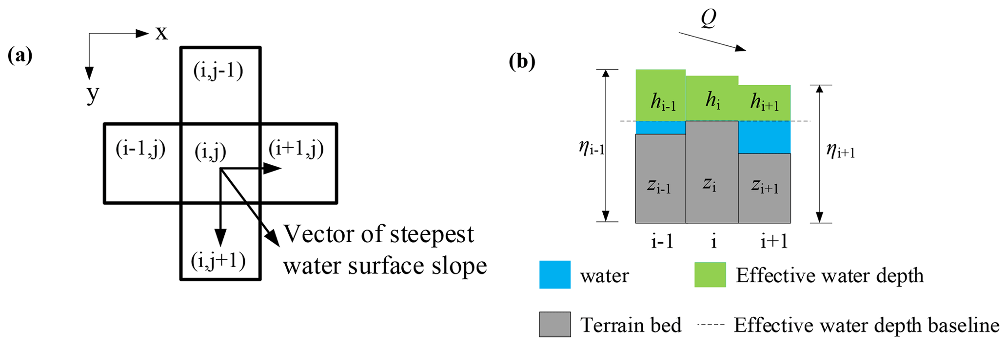
Compared to gravitational and frictional effects, the influence of acceleration and inertial terms of overland flow is negligible (Chen et al., 2012; Hsu et al., 2000). Time-dependent terms in the original momentum equations are omitted and thus obtain the diffusive wave equations. The numerical scheme can be found in the JFLOW model (Bradbrook, 2006; Yu and Duan, 2014b, 2017). The full shallow water equations are reduced to the diffusive wave equations by omitting the time-dependent terms. The flow velocity only depends on the local water surface gradient and roughness, and the water depth is determined by water volume balance and discharge from the neighbour grids. As shown in Fig. 1a, the possible flow at one cell is linked to two adjacent cells at each time step.

$$\begin{array}{}\text{(5)}& Q_i={\displaystyle \frac{w{h}^{\mathrm{5}/\mathrm{3}}{S}_i}{n(S_i^{\mathrm{2}}+S_j^{\mathrm{2}}{)}^{\mathrm{1}/\mathrm{4}}}},Q_j={\displaystyle \frac{w{h}^{\mathrm{5}/\mathrm{3}}{S}_j}{n(S_i^{\mathrm{2}}+S_j^{\mathrm{2}}{)}^{\mathrm{1}/\mathrm{4}}}},\end{array}$$

where

$$\begin{array}{}\text{(6)}& {\displaystyle }{S}_i={\displaystyle \frac{{\mathit{\eta }}_{i,j}-{\mathit{\eta }}_{i\pm \mathrm{1},j}}{w}},S_j={\displaystyle \frac{{\mathit{\eta }}_{i,j}-{\mathit{\eta }}_{i,j\pm \mathrm{1}}}{w}},\text{(7)}& {\displaystyle }{h}_i={\mathit{\eta }}_{i,j}-max(z_{i,j},z_{i\pm \mathrm{1},j}),h_j={\mathit{\eta }}_{i,j}-max(z_{i,j},z_{i,j\pm \mathrm{1}}),\text{(8)}& {\displaystyle }h={\displaystyle \frac{h_i{S}_i^{\mathrm{2}}+h_j{S}_j^{\mathrm{2}}}{S_i^{\mathrm{2}}+S_j^{\mathrm{2}}}},\end{array}$$

where w is the width of the cell, S_i and S_j are the water surface slopes in the orthogonal direction of i and j respectively, h_i and h_j are the effective depths in the orthogonal direction of i and j respectively, η_i,j and z_i,j are the water surface level and the ground elevation (m) respectively, and h is the effective depth. The change of water depth in each cell is then calculated using the following equation:

$$\begin{array}{}\text{(9)}& \mathrm{\Delta }h={\displaystyle \frac{(\sum Q_{\mathrm{in}i,j}-\sum Q_{\mathrm{out}i,j}-Q_{\mathrm{m}})\mathrm{\Delta }t}{w}}.\end{array}$$

Figure 1 Typical grid and water depth definition.

2.3 Hydrodynamic model

The 2D shallow water equations are the most widely used in the hydrodynamic models for the inundation simulations (Bradbrook et al., 2004; Yu and Duan, 2014a, 2017). Neglecting the Coriolis force, wind resistance, and viscosity, the equations are composed of the continuity equation

$$\begin{array}{}\text{(10)}& {\displaystyle \frac{\partial h}{\partial t}}+{\displaystyle \frac{\partial hu}{\partial x}}+{\displaystyle \frac{\partial hv}{\partial y}}=Q_{\mathrm{m}}\end{array}$$

and the momentum equations

$$\begin{array}{}\text{(11)}& {\displaystyle }\begin{array}{rl}{\displaystyle \frac{\partial hu}{\partial t}}& +{\displaystyle \frac{\partial }{\partial x}}(h{u}^{\mathrm{2}}+{\displaystyle \frac{\mathrm{1}}{\mathrm{2}}}g{h}^{\mathrm{2}})+{\displaystyle \frac{\partial }{\partial y}}\left(huv\right)=-gh{\displaystyle \frac{\partial z}{\partial x}}\\ & -C^{\mathrm{2}}u\sqrt{u^{\mathrm{2}}+v^{\mathrm{2}}},\end{array}\text{(12)}& {\displaystyle }\begin{array}{rl}{\displaystyle \frac{\partial hv}{\partial t}}& +{\displaystyle \frac{\partial }{\partial x}}\left(huv\right)+{\displaystyle \frac{\partial }{\partial y}}(h{v}^{\mathrm{2}}+{\displaystyle \frac{\mathrm{1}}{\mathrm{2}}}g{h}^{\mathrm{2}})=-gh{\displaystyle \frac{\partial z}{\partial y}}\\ & -C^{\mathrm{2}}v\sqrt{u^{\mathrm{2}}+v^{\mathrm{2}}},\end{array}\end{array}$$

where u and v are velocities along the x and y directions (m s⁻¹) respectively, h is water depth (m), g is gravity acceleration (m s⁻²), z is bottom elevation (m), C is the Chezy coefficient representing roughness, and Q_m is the source term which equals rainfall rate minus infiltration rate (m s⁻¹).

These equations are solved using the finite volume method similar to TELEMAC (Ata et al., 2013), and the convection flux is calculated using the Harten, Lax, and van Leer (HLL) scheme with the weighted average flux (WAF) approach (Toro, 2001).

$$\begin{array}{}\text{(13)}& F^{\mathrm{hll}}=\left\{\begin{array}{ll}{F}_{\mathrm{L}}& S_{\mathrm{L}}\ge \mathrm{0}\\ \frac{S_{\mathrm{R}}{F}_{\mathrm{L}}-S_{\mathrm{L}}{F}_{\mathrm{R}}+S_{\mathrm{L}}{S}_{\mathrm{R}}(U_{\mathrm{R}}-U_{\mathrm{L}})}{S_{\mathrm{R}}-S_{\mathrm{L}}}& S_{\mathrm{L}}\le \mathrm{0}\le S_{\mathrm{R}}\\ F_{\mathrm{R}}& S_{\mathrm{R}}\le \mathrm{0}\end{array}\right.,\end{array}$$

$$S_{\mathrm{L}}=U_{\mathrm{L}}-\sqrt{g{h}_L},S_{\mathrm{R}}=U_{\mathrm{R}}+\sqrt{g{h}_R},$$

where U_L, U_R, h_L, and h_R are the components of the left and right Riemann states respectively for a local Riemann problem; S_L and S_R are estimations of the speeds of the left and right waves respectively; and F^hll represents the fluxes in the star region. Using this flux, the WAF method of a second-order accuracy in time and space is achieved:

$$\begin{array}{}\text{(14)}& F_{i+\frac{\mathrm{1}}{\mathrm{2}}}=\sum _{k=\mathrm{1}}^{N+\mathrm{1}}{\mathit{\beta }}_k{F}_{i+\frac{\mathrm{1}}{\mathrm{2}}}^{\left(k\right)},\end{array}$$

$${\mathit{\beta }}_k={\displaystyle \frac{\mathrm{1}}{\mathrm{2}}}(c_k-c_{k-\mathrm{1}}),c_k={\displaystyle \frac{\mathrm{\Delta }t{S}_k}{\mathrm{\Delta }x}},c_{\mathrm{0}}=-\mathrm{1}\mathrm{and}{c}_{N+\mathrm{1}}=\mathrm{1},$$

where $F_{i+\frac{\mathrm{1}}{\mathrm{2}}}^{\left(k\right)}=F\left(U^{\left(k\right)}\right)$, N is the number of waves in solving the Riemann problem, and β corresponds to the differences between the Courant numbers c_k of successive wave speeds S_k.

The topography term on the right side of Eqs. (11) and (12) is calculated by the hydrostatic reconstruction scheme:

$$\begin{array}{}\text{(15)}& -gh{\displaystyle \frac{\partial z}{\partial x}}=\mathrm{\nabla }{\displaystyle \frac{g{h}^{\mathrm{2}}}{\mathrm{2}}}={\displaystyle \frac{g}{\mathrm{2}}}{\displaystyle \frac{\mathrm{\Delta }t}{\mathrm{\Delta }x}}\left[\right(h_i^R{)}^{\mathrm{2}}-\left(h_i^L{)}^{\mathrm{2}}\right],\end{array}$$

$$\left\{\begin{array}{l}{h}_i^R=\max [\mathrm{0.0},h_i+z_i-\max (z_i,z_{i+\mathrm{1}}\left)\right]\\ h_i^L=\max [\mathrm{0.0},h_i+z_i-\max (z_{i-\mathrm{1}},z_i\left)\right]\end{array}\right..$$

The friction term is computed by a semi-implicit scheme to ensure numerical stability (Liang et al., 2007):

$$\begin{array}{}\text{(16)}& (hu{)}^{n+\mathrm{1}}={\displaystyle \frac{(hu{)}^n}{\mathrm{1}+\mathrm{\Delta }t(\frac{g\sqrt{(hu{)}^{\mathrm{2}}+(hv{)}^{\mathrm{2}}}}{h^{\mathrm{2}}{C}^{\mathrm{2}}}{)}^n}}.\end{array}$$

The time step is determined under the Courant–Friedrichs–Lewy (CFL) condition as follows.

$$\begin{array}{}\text{(17)}& \mathrm{\Delta }t=C_r\min ({\displaystyle \frac{\mathrm{\Delta }{x}_i}{\left|u_i\right|+\sqrt{g{h}_i}}},{\displaystyle \frac{\mathrm{\Delta }{y}_i}{\left|v_i\right|+\sqrt{g{h}_i}}}),\end{array}$$

where C_r is the Courant number, limited by $\mathrm{0}<C_r\le \mathrm{1}$ for simulation stability, and a typical value of 0.9 is used for the following simulation cases. More details of the numerical schemes can be found in Ata et al. (2013).

2.4 Coupling approach

The computation domain in the DBCM is divided into non-inundation and inundation regions, and the diffusion wave equation (DWE) is solved in the non-inundation regions with small water depth while the hydrodynamic model full shallow-water equations (SWEs) is applied in the inundation regions with high water depths. The model for a specific grid is determined based on its local and neighbouring flow states. The boundary between the non-inundation regions and inundation regions forms a dynamic coupling boundary which is time-dependent. In addition, special treatment on discharge through the coupling boundary needs to be carried out based on the local flow state using the characteristic theory.

Figure 2 Schematic diagram of DBCM.

Figure 3 Flow state change and position of the coupling boundary.

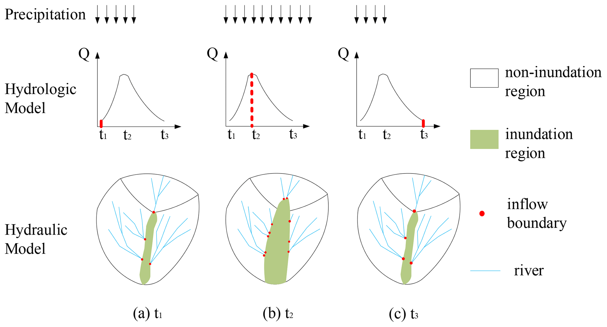
The adopted models for different regions are based on the temporally evolving flow statuses. They lead to the change in coupling boundary positions. As shown in Fig. 2, when the rainfall intensity increases, the inundation region expands as a consequence of the gradually accumulating surface water volume from upstream regions. The position of the in-flow boundary, flow path, and discharge change subsequently. The coupled models proposed by other researchers, either UCM or BCM, did not fully consider this phenomenon.

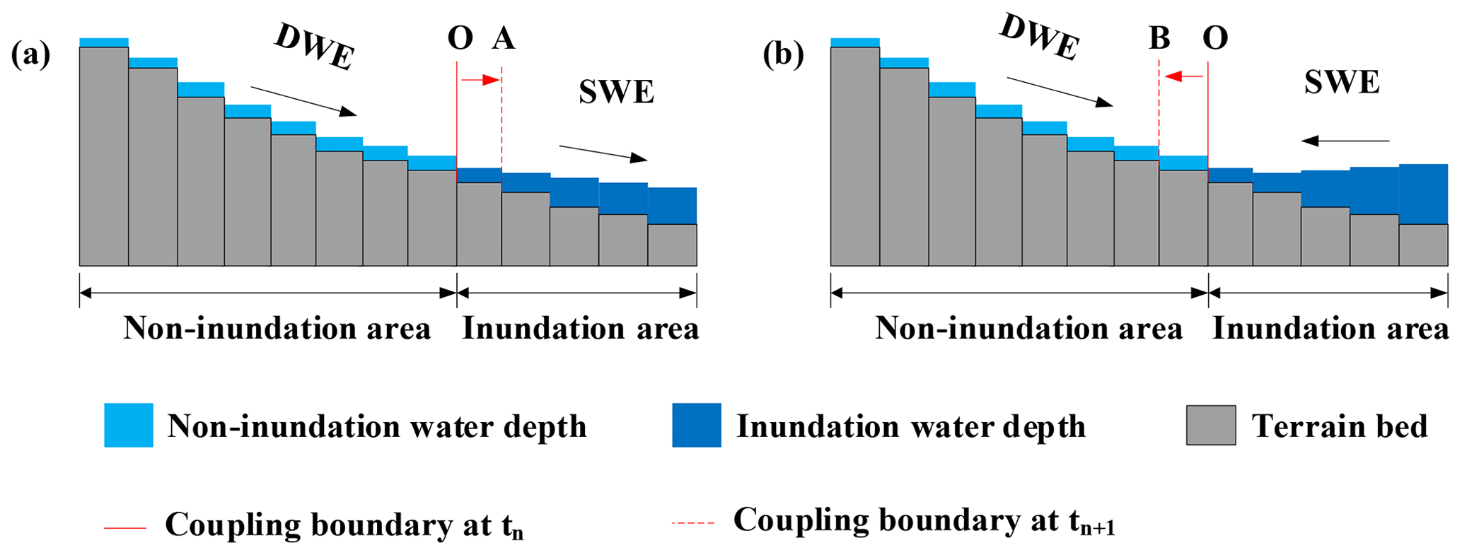
Figure 3 shows a detailed process of flow state change on both sides of the coupling boundary. For the case in Fig. 3a, the discharge on the coupling boundary equals the upstream discharge and is not affected by the downstream flow, which means that the local discharge is completely determined by the DWE. After the water depth is updated, the location of the coupling boundary point O moves to point A according to the comparison of its water depth to the water depth threshold. Moreover, the flow in the inundation region may move from downstream to upstream, as shown in Fig. 3b. The discharge and water depth on the coupling boundary should be determined using the flow information on both sides. In this case, the coupling boundary moves to point B due to inundation area expansion.

In previous studies, the discharge on the coupling boundary has been computed directly through the hydrologic model, using empirical formulae, or by interpolation approaches according to the water level or velocity gradient on both sides. Such methods may fail to provide an overall understanding of the flow regime status of the combined hydrologic and hydrodynamic model. In using the DBCM, the following procedures are conducted at the coupling boundary: the flow state is obtained by both the hydrologic and hydrodynamic models in their local grids, then the discharge through the coupling boundary is computed, and the entire water depth is updated according to the water volume variation. After that, the location of the coupling boundary is updated and the area of the non-inundation region and inundation region is remapped. The key issue using the DBCM is to establish a reasonable approach to determine the discharge on the coupling boundary, which should integrate the effect of current flow state obtained by the two models on both sides of the coupling boundary.

Figure 4 Direction of characteristic wave.

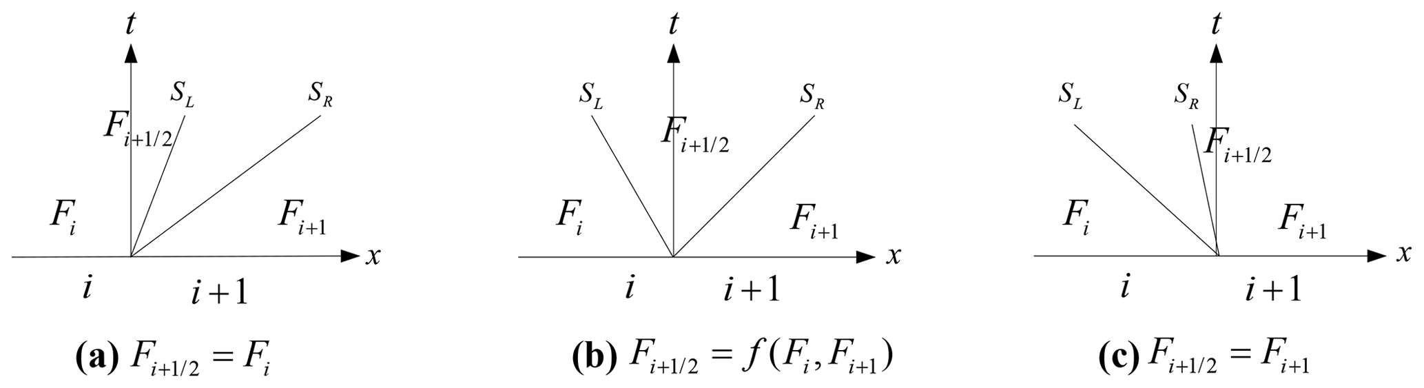
According to Godunov theory (Godunov, 1959), the solution of convective flux implementing the finite volume method can be considered a local Riemann problem. The discontinuity characteristic speed between each grid represents the propagation of local fluid variables in time and space, as shown in Fig. 4. When the characteristic speeds are all positive, the flux depends entirely on the left-side flow state, and vice versa. However, when the characteristic speeds have a negative value and a positive value, the current flow state in both grids must be taken into consideration. Applying this approach to DBCM, the computational scheme at the boundary can be specified. It is known that the hydrologic model only transfers water mass, while the hydrodynamic model transfers both water mass and momentum. More details of the different coupling cases are shown in Fig. 5.

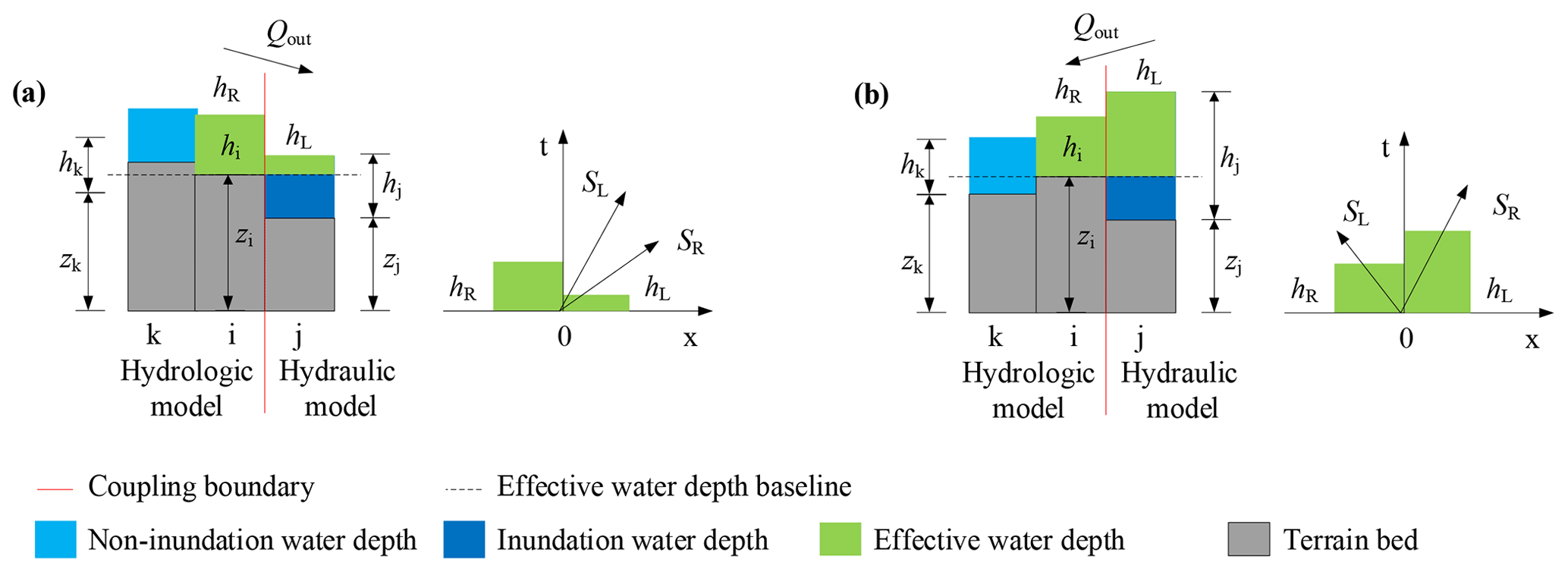
Figure 5 Coupling conditions; the discharge at the coupling boundary depends on (a) the hydrologic model and (b) both hydrologic and hydrodynamic models.

For the first case in Fig. 5a, the hydrologic and hydrodynamic models are calculated independently, corresponding to the situation in which positive bed slopes induce confluence flows into the river. Thus only the discharge calculated by the hydrological model passes through the coupling boundary (Fig. 3a). The flow information in grid k and i is calculated using DWE and grid j using SWE; see Fig. 5a. Firstly, a slope analysis of DWE is conducted uniformly. Obviously the water level gradient between grid k and grid i is smaller than that between grid i and grid j. According to the calculation results from the DWE, the velocity points to the direction with the maximum water level slope (in Fig. 1a, flow directs to the right). Therefore, the change of water depth in grid k has nothing to do with the flow state at grid i, and the velocity change at grid k is analysed by the other grids on the left of grid k. The flow information at grid i and j forms a local Riemann problem and then the characteristic speed is analysed. The velocity at grid i is obtained from the above analysis, and the velocity at grid j is the velocity at the current moment. The water depths at the discontinuity interface are calculated as $h_i^r=h_i+z_i-\max (z_i,z_j)$, $h_j^l=h_j+z_j-\max (z_i,z_j)$. Thus a pair of characteristic waves at the interface are obtained:

$$\begin{array}{}\text{(18)}& S_{\mathrm{L}}=u_i-\sqrt{g{h}_i^R},S_{\mathrm{R}}=u_j+\sqrt{g{h}_j^L}.\end{array}$$

When the characteristic speeds $S_{\mathrm{R}}\ge S_{\mathrm{L}}>\mathrm{0}$, the flux calculation depends on the flow information at grid i, independent of grid j. The velocity at grid i is calculated using diffusion wave equations and only outflow is allowed. In addition to the water depth change calculated according to the hydrodynamic model at grid j, the water volume transferred from grid i should also be added. No convection term in the momentum equation of DWE indicates no momentum transfer between grids i and j, and thus the velocity values of the two grids do not interact with each other.

For the second case in Fig. 5b, the hydrological model and hydrodynamic model are both used, corresponding to the situation when the inundation area expands (Fig. 3b). As shown in Fig. 5b, the water depth in grid k and grid i is small; thus the hydrologic model is applied. While grid j has a deep water depth and high water elevation, the hydrodynamic model is applied. In this case, the velocity direction is from grid i to grid k. The characteristic wave analysis at the interface of grid i and grid j reveals that $S_{\mathrm{R}}>\mathrm{0}>S_{\mathrm{L}}$, which means that the momentum at grid j can be transferred to grid i. Grid i is involved in the computational domain of the hydrodynamic model. The water depth increment at grid i needs to deduct the current discharge output to grid k and the flow rate obtained by solving the hydrodynamic equation with the flow state at grid j. The velocity increment at grid i is obtained by solving the hydrodynamic equation with the flow state at grid j based on current velocity. Then the flow state at grid i is updated and the coupling boundary position may change when the depth varies.

The slope gradient analysis and characteristic wave analysis are key issues of the computational theory for solving DWE and SWE respectively. The key to coupling these two approaches is to successfully address the connection on the coupling boundary. As discussed earlier, in existing studies only one governing equation is solved throughout the computational domain, but it cannot consider the interaction between the two kinds of governing equations and resize the area of a different computational domain. A reasonable and implementable approach in coupling the solution procedure of DWE and SWE is the precondition for establishing DBCM. In this study, the slope gradient analysis is performed to determine the current velocity together with the current water depth, and the characteristic wave analysis is conducted on the coupling boundary as long as flow velocity and depth have been provided, no matter whether it is calculated from the hydrologic or hydrodynamic model. Then, the flow information exchange on the coupling boundary is determined according to the characteristic speed which reflects the propagation of flow state in time and space. This method integrates the hydrologic model and hydrodynamic model into a comprehensive system by means of joining the two steps of slope gradient analysis and characteristic wave analysis.

In the proposed DBCM, the coupling boundary position will not stay fixed in advance throughout the calculation process. The location where the runoff enters the inundation region varies dynamically, and the flood level can also submerge the original inflow points and regenerate new coupling boundaries. Such an alternation mechanism is close to natural flow processes. The characteristic wave theory is used to determine the mass and momentum exchange through the coupling boundary. Compared to the “cascade” operation in UCM, the present DBCM solves DWE and SWE simultaneously. When non-inundation regions get larger, the flow movement is mainly obtained by utilizing DWE. Whereas when the inundation regions extend, the computational domain is given priority to SWE.

3 Model validation

The numerical model results from DBCM are compared with analytical solutions, experimental data, and results obtained from existing numerical models. Considering the complexity of the numerical model schemes used in the hydrologic and hydrodynamic models, the hydrodynamic model performance will be validated in the first stage, and then the performance of DBCM will be verified using a V-shaped catchment. As described in Sect. 2.2, the numerical schemes of the hydrodynamic model (referred to as HM2D in the following section) used in this study have second-order accuracy in both time and space.

Figure 6 Oblique hydraulic jump: definition sketch.

3.1 Oblique hydraulic jump

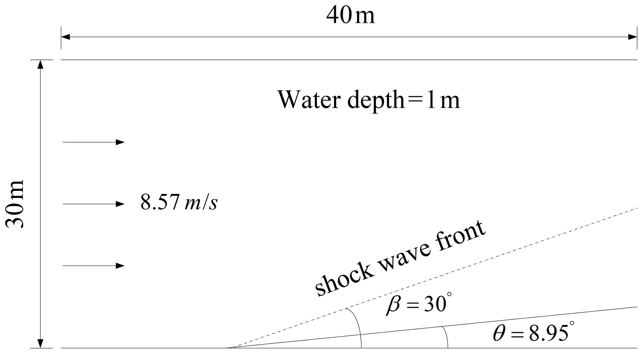
The oblique hydraulic jump example is a special flow pattern, with an analytical solution being available in open channel flows, which is often used to verify the capability of the numerical schemes in simulating shock wave formation. When a supercritical flow is deflected by a converging wall at an angle θ, the resulting shockwave forms an oblique hydraulic jump at an angle β, as depicted in Fig. 6. Both the angles of water surface lines behind the shock wave front can be obtained by an analytical solution. In this study, the upstream flow water depth and velocity are set as 1 m and 8.57 m s⁻¹, and the oblique angle $\mathit{\theta }=\mathrm{8.95}{}^{\circ }$. The width and length of the channel are 30 and 40 m respectively. In these conditions, the exact analytical solutions are downstream water depth D_A=1.49984 m, downstream velocity V_A=7.95308 m s⁻¹, and angle $\mathit{\beta }=\mathrm{30}{}^{\circ }$ (Rogers et al., 2001) when the flow reaches a steady state.

Figure 7 Steady state of water depth of oblique hydraulic jump.

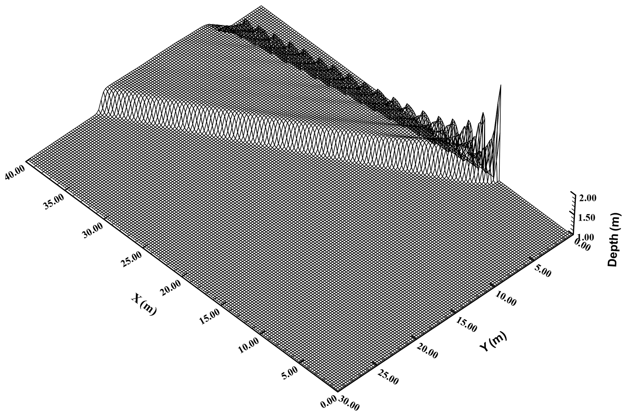
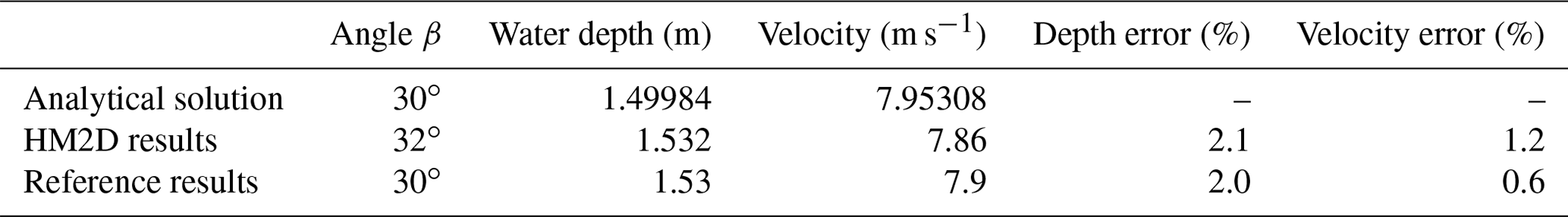
The spatial step size is set as $\mathrm{\Delta }x=\mathrm{\Delta }y=\mathrm{0.33}$ m. The time step is dynamically adjusted and the total calculation time is 90 s. Figure 7 shows a 3D view of the water depth of results predicted by our model. The oblique jump is sharply captured and has an angle $\mathit{\beta }\approx \mathrm{32}{}^{\circ }$. The average water depth downstream behind the shock front is 1.532 m, and the average velocity is 7.86 m s⁻¹. The numerical solution is close to the analytical solution, as shown in Table 1. The output of HM2D and the references, either the water depth or velocity, show good agreement (see Table 1).

Table 1 Comparison between the analytical solution and calculation result for the oblique jump case.

3.2 Dam break over a dry flood plain

Dam break is a classic benchmark problem, which is often used to verify the capability of a numerical scheme in dealing with the dry–wet boundary, and the physical experimental model is easy to conduct. Thus, it is convenient to collect experimental data for comparison with numerical results. The experiment performed by Fraccarollo and Toro (1995) was used to validate the DBCM developed in this study. The model domain is 3 m × 2 m, which is separated into two areas by a dam at X=1 m. Initially, the still water with a depth of 0.64 m in the reservoir is surrounded by solid walls, while the downstream area is initially dry. The boundaries of the downstream floodplain were all open. A 0.4 m wide section in the middle of the dam was breached instantaneously. The numerical model spatial step is $\mathrm{\Delta }x=\mathrm{\Delta }y=\mathrm{0.04}$ m, and the roughness coefficient is n=0.01.

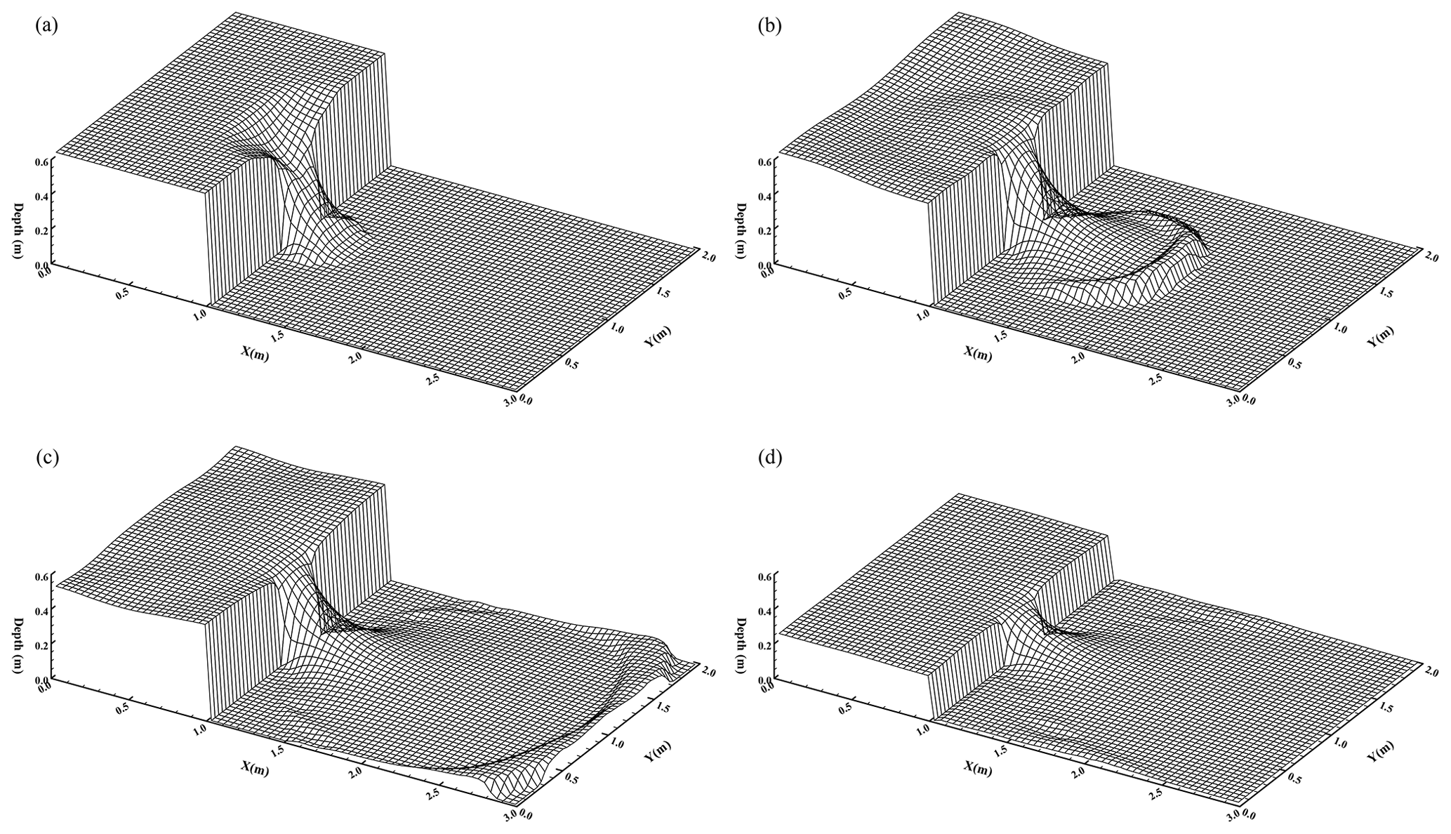
Figure 8 Snapshot of the water elevation for dam-break simulation: (a) t=0.1 s; (b) t=0.5 s; (c) t=1.1 s; (d) t=5.0 s.

Figure 8 shows the water surface elevation at different times. It can be clearly seen that the bore wave initially propagates downstream. A depression wave travels upstream, which is reflected back at the walls surrounding the reservoir, causing the water surface elevation in the reservoir to oscillate. In Fig. 9, a comparison between the measured and the computed data is made, which shows a good agreement. The results are encouraging and the overall trend is well captured.

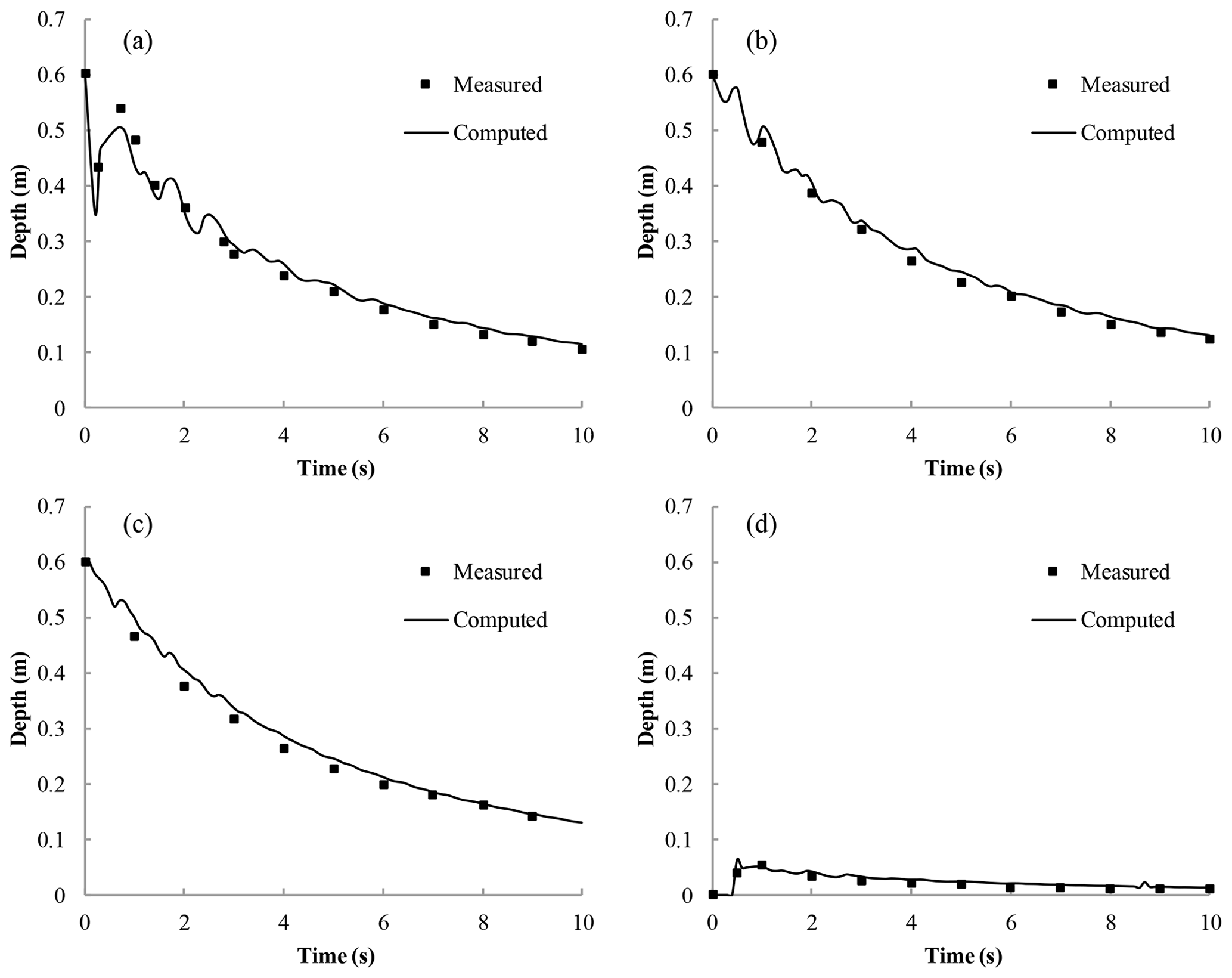
Figure 9 Comparison of water depth variation at four locations: (a) x=1 m, y=1 m; (b) x=0.18 m, y=1 m; (c). x=0.48 m, y=0.4 m; (d) x=1.802 m, y=1.45 m.

3.3 Two-dimensional surface flow over a tilted V-shaped catchment

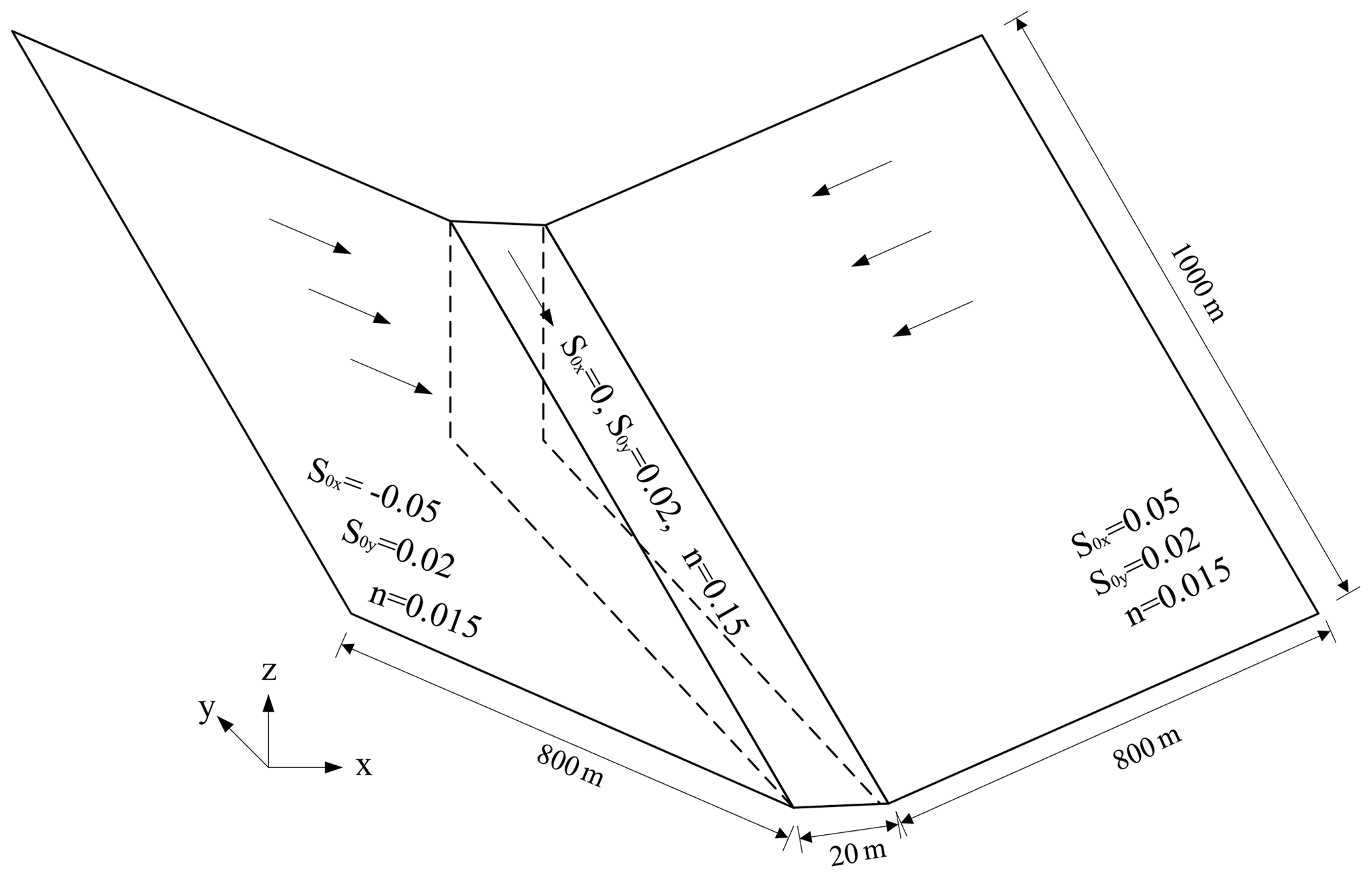
A two-dimensional surface flow over a tilted V-shaped catchment is simulated (Di Baldassarre et al., 1996; Panday and Huyakorn, 2004). We aim to verify whether the computational domains of the hydrologic and hydraulic models can dynamically switch and compare the difference between DBCM, UCM, and BCM. As shown in Fig. 10, the topography of the example is depicted.

The computational domain is symmetrically V-shaped, with a pair of symmetrical hillslopes forming a channel at the central region. The bed slopes are ±0.05 spanwise and 0.02 streamwise parallel to the channel. The manning coefficient on the hillslope is 0.015 while it is 0.15 in the main channel. The total simulation time is 180 min and the constant rainfall intensity is 10.8 mm h⁻¹ for 90 min. Figure 10 shows the detailed dimension and related information of the V-shaped catchment.

Figure 10 Diagram and dimension of the tilted V-shaped catchment.

Considering the hydrodynamic model provides more details to describe the overland flow than the hydrologic model, the HM2D and DBCM under the same rainfall conditions were adopted. When water depth is less than 0.005 m, the grid is calculated using the hydrological model, and when water depth is greater than 0.005 m the grid is applicable to the hydrodynamic model. Results are compared with numerical models developed by Di Baldassarre et al. (1996) and Panday and Huyakorn (2004).

Figure 11 Comparison of discharge hydrographs of the V-shaped catchment.

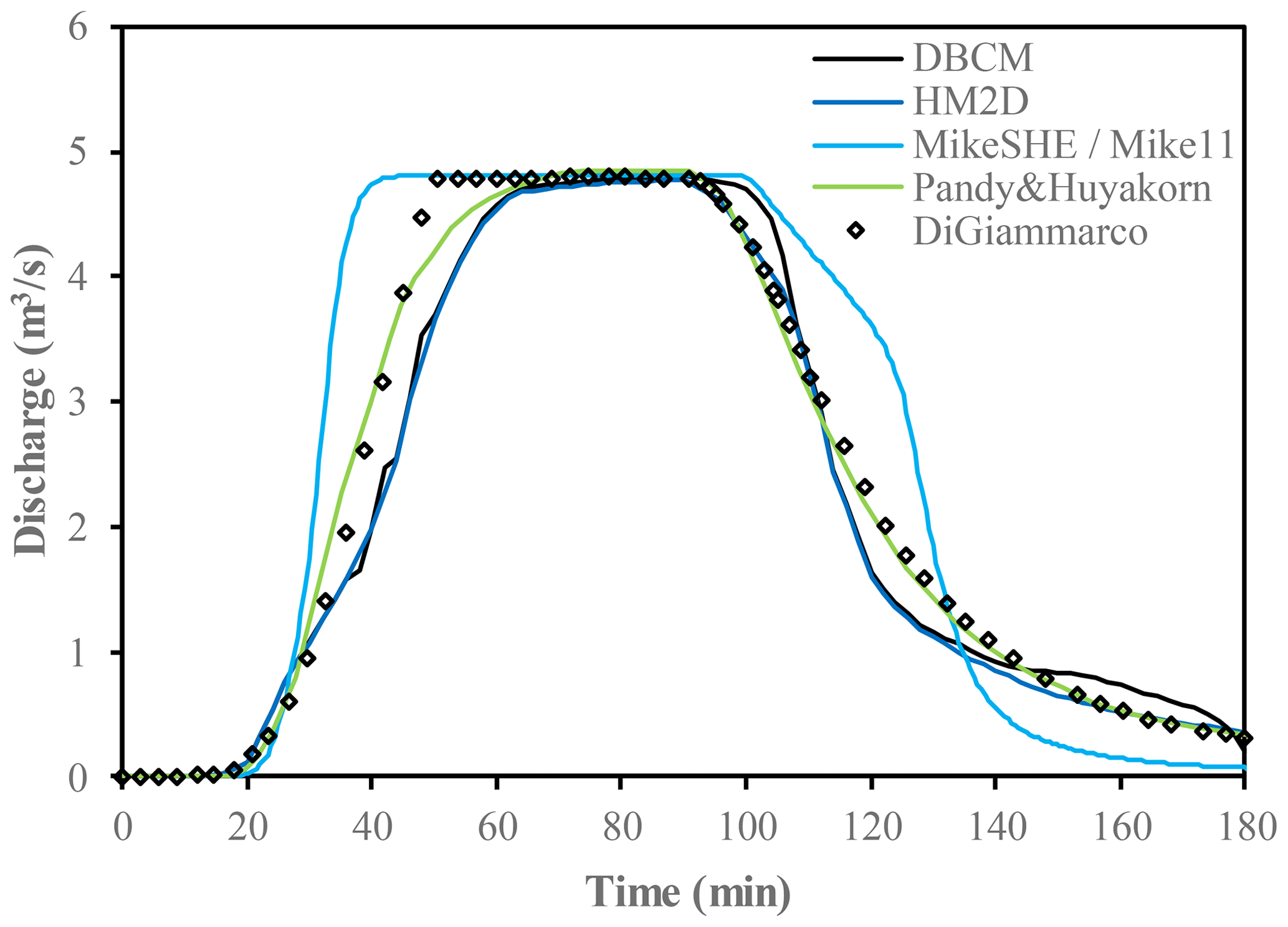
As shown in Fig. 11, the discharge hydrographs obtained by the HM2D and DBCM are compared with other existing models. The discharge hydrographs show good agreement for the peak discharge. The start periods of discharge rising and receding limbs simulated by HM2D and DBCM are consistent with those predicted by others. However, discrepancies gradually grow, and both the HM2D and DBCM slightly under-predict the discharge. Despite this disparity, the overall trend of the hydrographs indicates that the proposed models are satisfactory.

Comparing the hydrographs between the HM2D and DBCM, it can be seen that their rising limb and peak discharges agree very well. Consequently, both these hydrodynamic models are used to simulate the overland flows. The difference between HM2D and DBCM gradually emerges at the receding limb. The HM2D simulates water movement using the hydrodynamic model (SWE) throughout the computation process, while the DBCM switches from the hydrodynamic model to the hydrologic model (DWE) when the upstream water depth falls below the threshold. Since there are no inertial terms in the hydrologic model, the velocity at the present is a function of the current water level gradient and is not equal to the velocity at the previous moment plus the flux term. For this reason, when the DBCM switches from the hydrodynamic model to the hydrologic model, and the velocity calculation approach changes accordingly, then the discharge difference between the HM2D and DBCM emerges. Therefore, the outlet flow is slightly larger, but later slightly smaller, in the DBCM, assuring overall the mass is conserved.

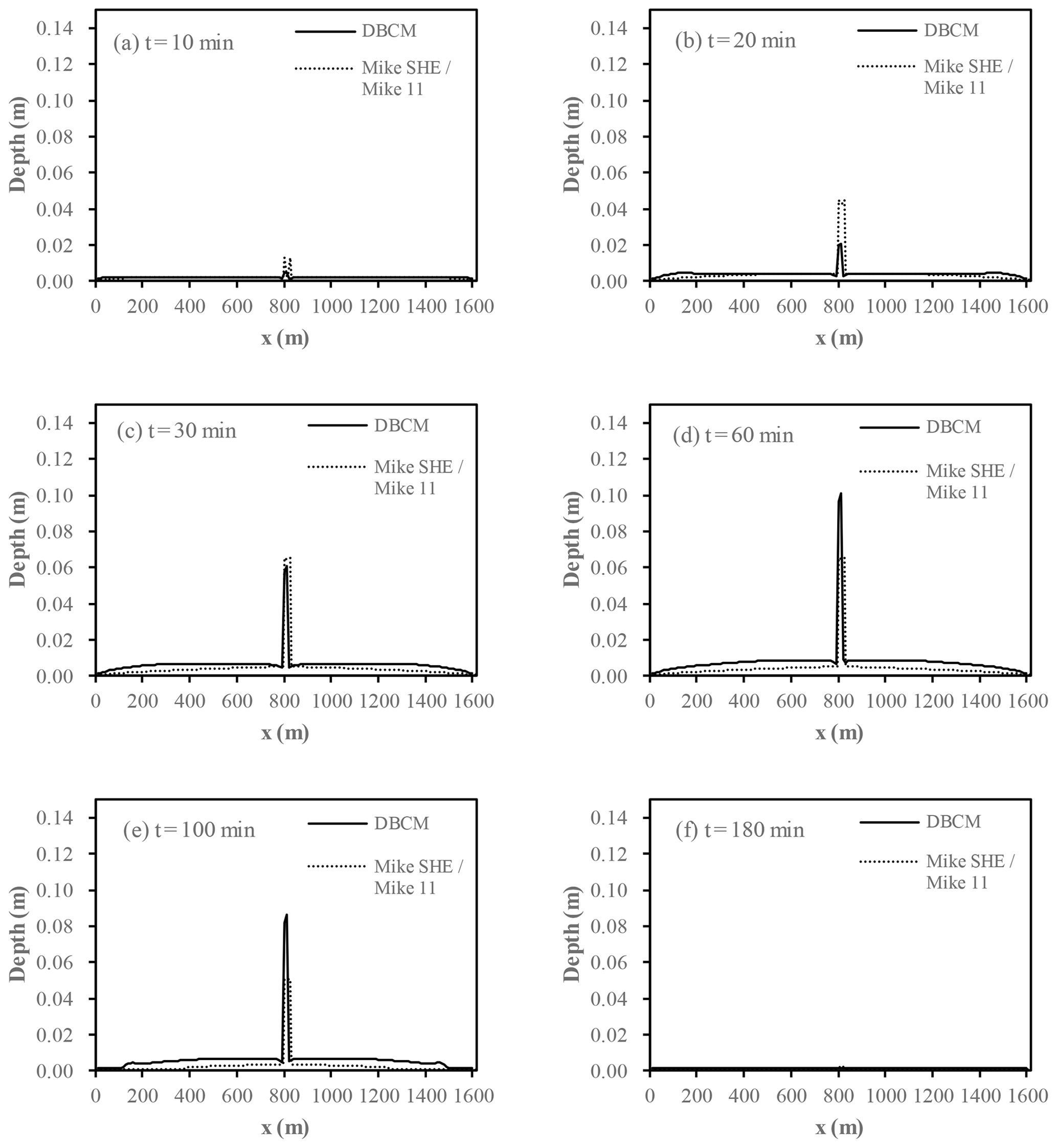
Figure 12 Comparison of water depth profile between DBCM and MIKE SHE–MIKE 11 at the downstream catchment (y=500 m).

In order to make a detailed performance between DBCM and BCM, the coupled model of MIKE SHE and MIKE 11 was used to conduct the comparison with the proposed DBCM. The coupling between MIKE SHE and MIKE 11 is achieved using the line segments termed river links (Thompson et al., 2004). Water can exchange between MIKE 11 H-points and adjacent MIKE SHE river links, and in this way the bidirectional coupling between the two models is realized. The coupling use the overbank spilling option, when the water level is over the riverbank top elevation, then the overland flow to the river is added to MIKE 11 as lateral inflow. Conversely, when the water level in the river is higher than that of overland flow, the water from the main river will spill into the MIKE SHE cell and become part of the overland flow. However, the MIKE SHE river links and MIKE 11 H-points are pre-processed before the simulation starting, which means they are determined automatically and stay fixed during the simulation, and the flow information between them uses the method of interpolation. In addition, MIKE SHE only exchanges water volume with the coupled reaches and keeps the water balance in river links, which is not the case in actual rainfall events for which the water exchange should always be dynamical and successive.

Figure 12 shows the comparison of water depth profile (y=500 m) between DBCM and MIKE SHE–MIKE11. It can be found that water depth shows a small difference on the overland slope. Flood propagation is a phenomenon of high-speed movement resulting in a drastic change of water depth and velocity. The hydrologic model (DWE, omitting convection term) is insufficient to describe this movement. However, the water depth near the outlet presents the difference of the two models. In the first 30 min, the water depth from DBCM was lower than the water depth from the MIKE SHE–MIKE11 model. After that until the end of the simulation, the water depth from DBCM was higher than the water depth from the MIKE SHE–MIKE 11 model. The increase in water depth around the channel leads to strong convective flow; thus the momentum transfer needs to be taken into consideration in order to get reasonable simulation results. However, the momentum transfer is not taken into account in the MIKE SHE–MIKE 11 coupled model.

Figure 13 Discharge processes in the centre channel.

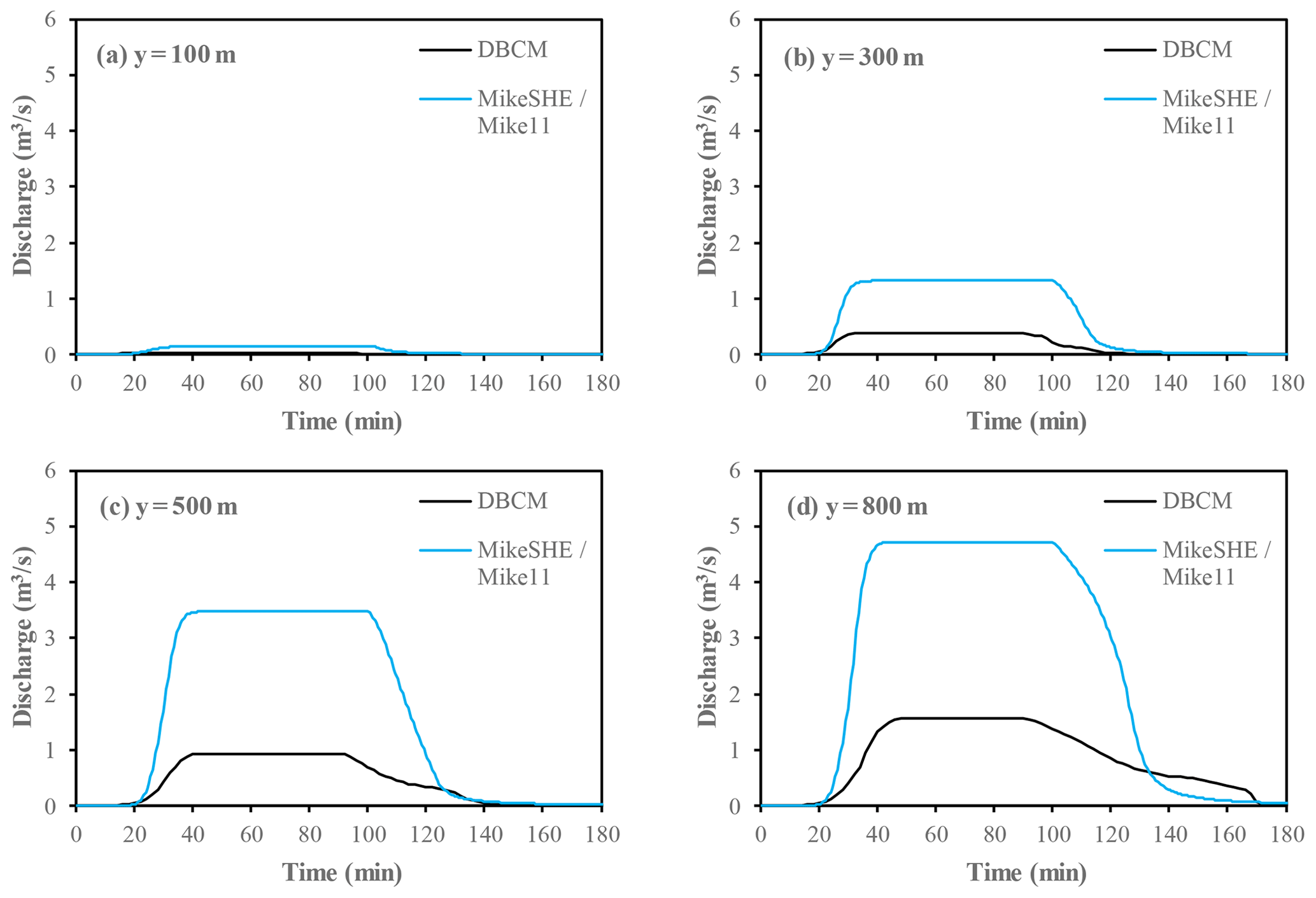
Flow discharge of the centre channel is shown in Fig. 13. It can be found that discharge in the channel obtained by DBCM is much lower than that obtained by the MIKE SHE–MIKE 11 coupled model. This is due to the difference of coupling mechanism and flow information exchange. Flow can only be exchanged between the finite river links and H-points, and flow from overland can accumulate around the river links, which leads to a relative increase in flow discharge. In terms of the DBCM, the flow can exchange water information, including both mass and momentum, with the dynamical coupling boundary. The coupling mechanism of DBCM shows accordance with natural physical processes of flood formation and propagation.

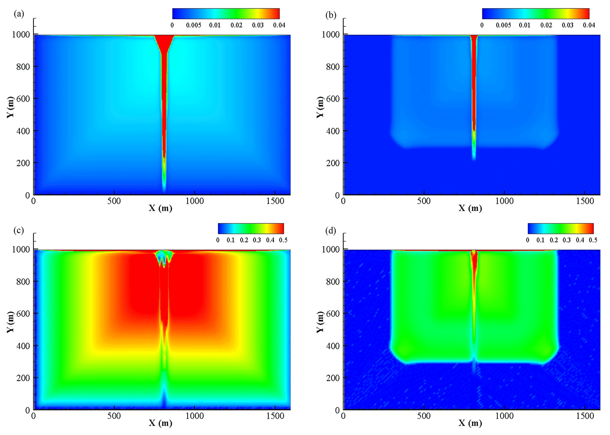
Figure 14 Water depth (m) and velocity distribution (m s⁻¹) at 90 min (a, c) and 120 min (b, d).

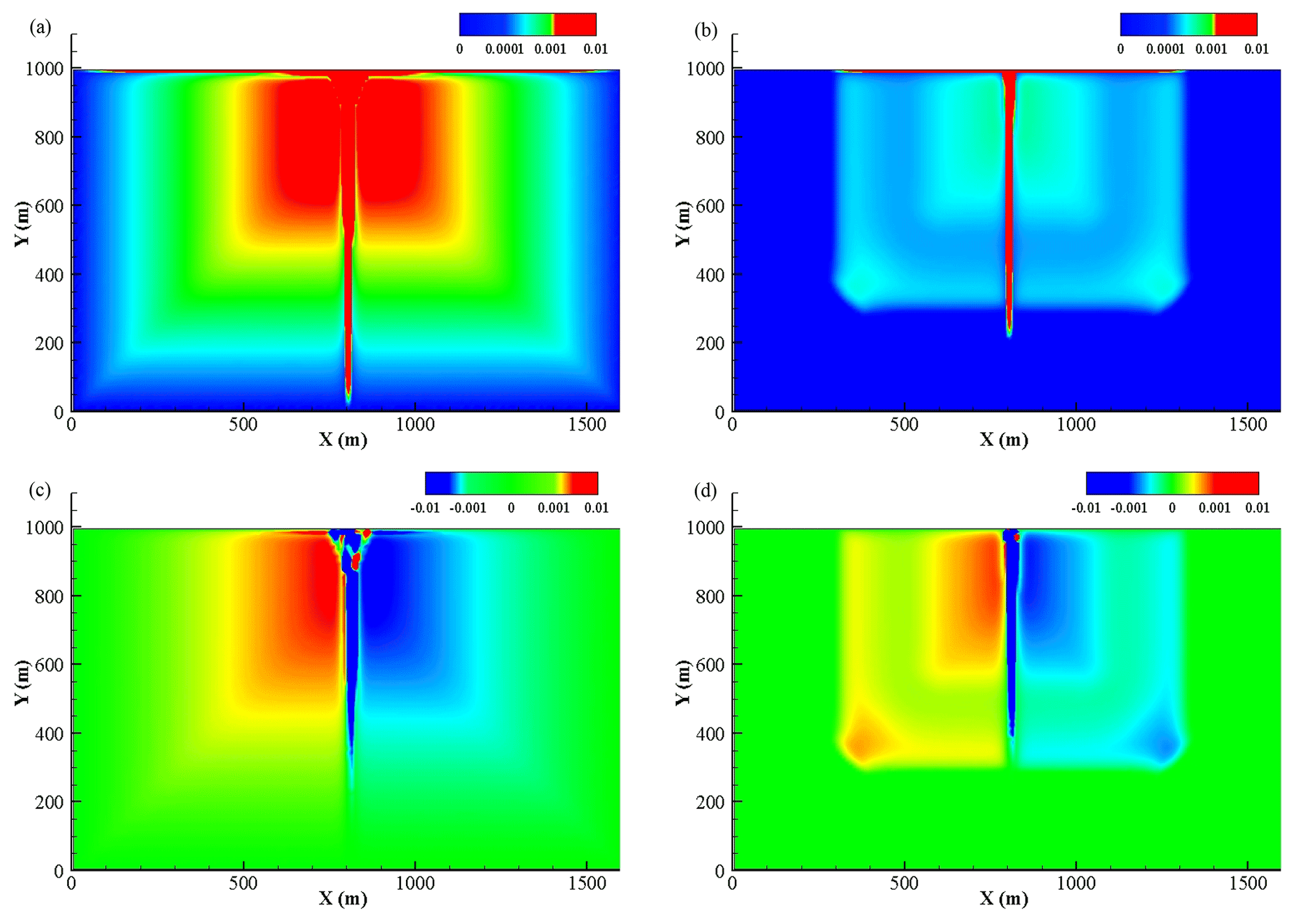
Figure 15 Flux (m⁴ s⁻²) distributions in X and Y direction at 90 min (a, c) and 120 min (b, d).

The spatial variability of the flow depth, velocity and flux at 90 and 120 min is shown in Figs. 14 and 15. For the DBCM, the main difference between the governing equations used by the hydrologic model and hydrodynamic model is that the flux term is not calculated in the former; meanwhile the latter needs to calculate the convection term. The non-inundation region and inundation region can be determined by whether the flux term is generated during the calculation process. When t=90 min, the rain stops, the water depth reaches its peak value, and the flow information is determined by the hydrodynamic model over the whole domain. At t=120 min, the water continues to flow to the outlet and the water volume near the upstream region decreases, but a small amount of water still exists. No flux is calculated while velocity computation continues. Obviously, a sharp division line separating the domain arises at this moment.

Figure 16 Evolution of coupling boundary.

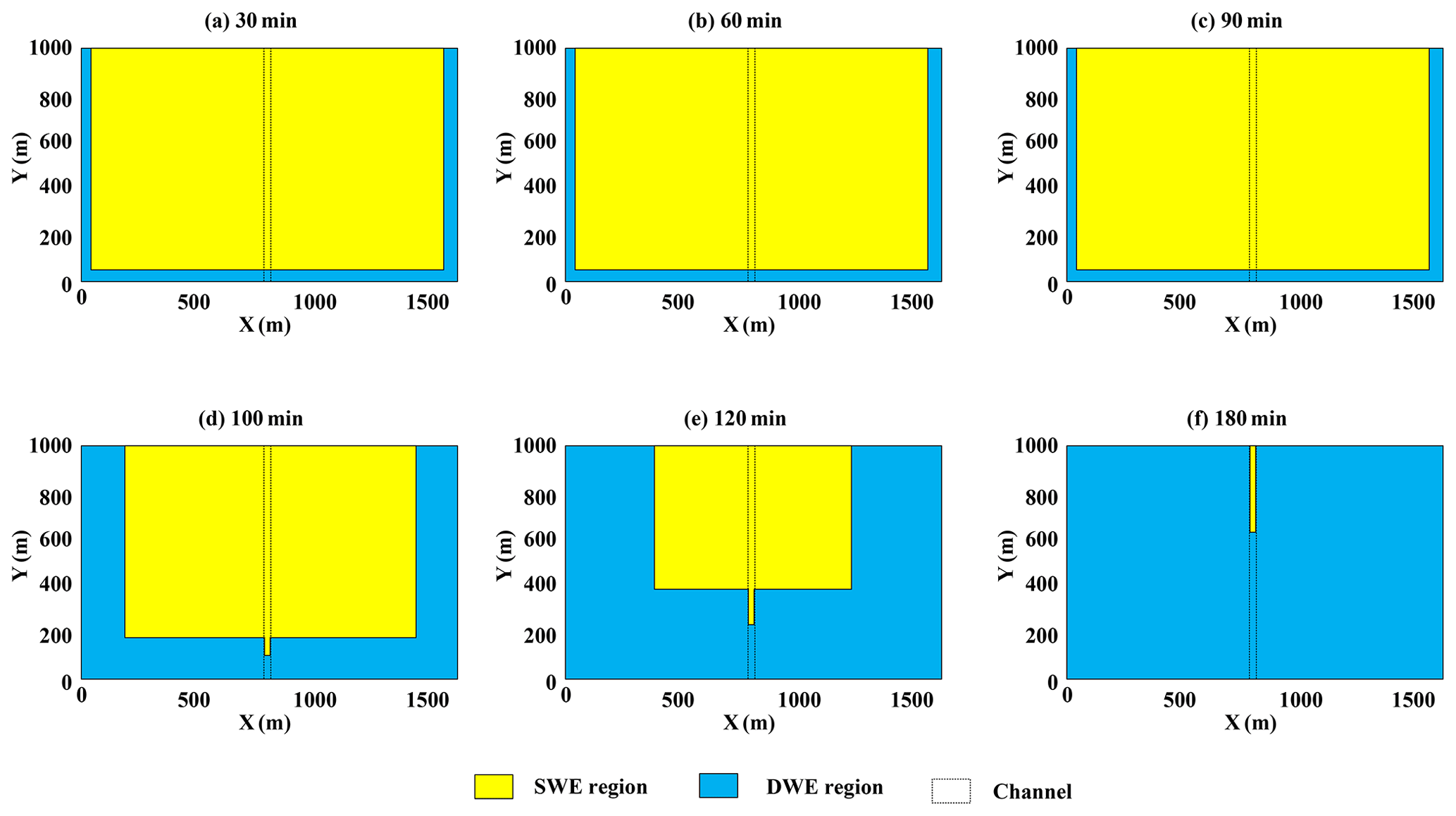
For the DBCM, the coupling boundary between DWE and SWE is time-dependent. Figure 16 shows the evolution of the coupling boundary. During the first 90 min, rainfall stays constant over the whole catchment and water depth rises in a short period. As a result, the water depth in most of the domain is above the depth threshold and SWE was implemented in these regions. However, 90 min later, the rainfall stops and no extra water flows into the domain. Then, the water depth begins to decrease. Once the depth is lower than the depth threshold, the grid cell uses DWE to determine the discharge as well as water depth and the coupling boundary shrinks (see Fig. 16). The evolution of coupling boundary is consistent with the flux analysis stated above.

Figure 17 Comparison of water depth profile in the channel outlet.

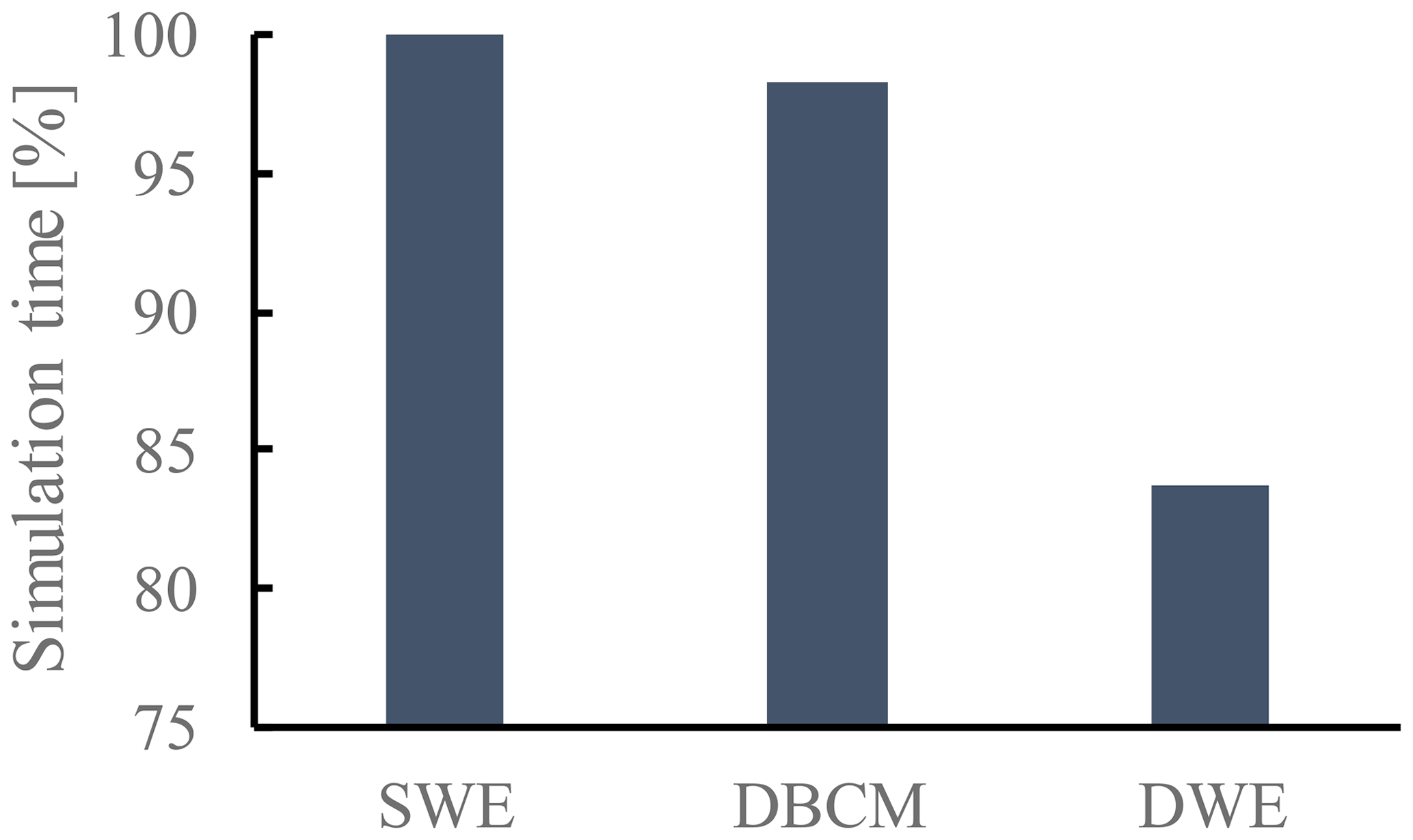
It is well known that solving the SWE costs numerous computational resources and time, which limits its application, especially for large-scale simulation. In terms of this small-scale V-shaped catchment, simulation performance between the SWE, DBCM, and DWE was evaluated. Figure 17 shows the result and the simulation time was used by the SWE (100 %). It can be seen that both the DBCM and DWE need less simulation time compared to SWE; for DWE nearly 15 % simulation time was saved. Whereas the DBCM alters the SWE and DWE according to the local flow information. Compared with SWE, the simulation time of DBCM was only slightly lower than the SWE due to the fact that in the early half of the simulation in this V-shaped catchment most of the flow information is calculated by the SWE as discussed in the above section (Fig. 16).

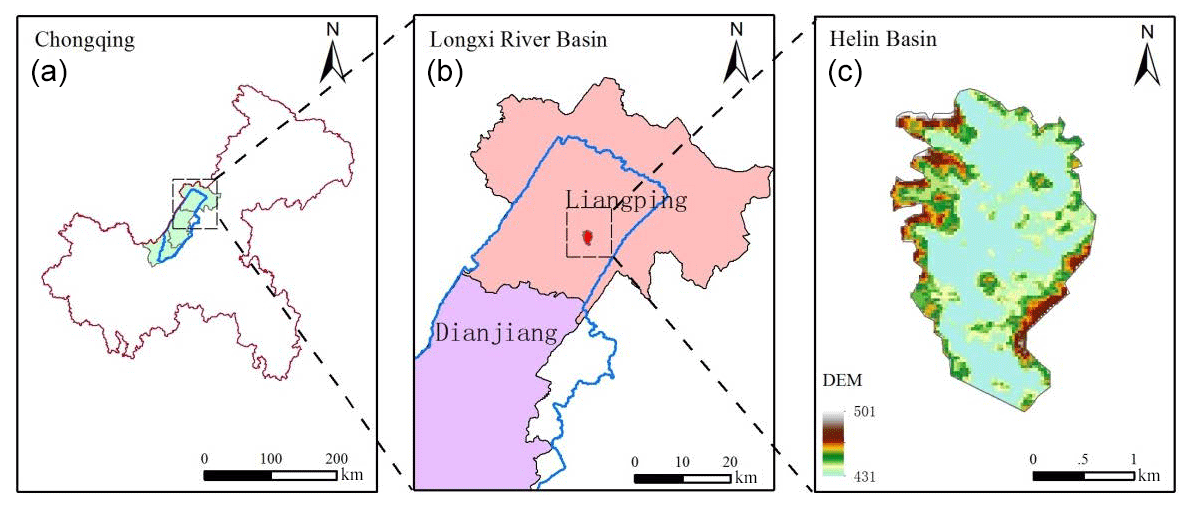
Figure 18 Location of Helin Town. Chongqing City (a). Longxi River basin (b). Helin basin (c).

4 DBCM implemented for a natural watershed

The proposed DBCM was implemented in a natural watershed for flood risk assessment, that is, Helin Town of Longxi River in Chongqing City, China. The Longxi river basin is located in the eastern region of Chongqing (see Fig. 18), which is a first-class tributary of the Yangtze River. It is about 221 km long with a catchment area of about 3280 km². The overall terrain gradually goes down from northeast to southwest, consistent with the trend of the main channel. Most of the central and southwest areas are relatively flat, and the east and west areas are mountainous, a typical topography of a trough sandwiched by two mountains. The average annual rainfall in the basin is 1192.4 mm, which is prone to heavy rain in summer, and the flood spreads rapidly to the central district due to the topographic feature. The selected catchment, Helin Town, located in the northeast of the Longxi River basin, was chosen as a case study for investigating the surface flow phenomena using the DBCM. The administrative location and DEM information of Helin Town are shown in Fig. 18.

The river section in Helin basin is a typical mountainous river. The upper part of the river has a steep slope, while the middle and lower reaches are relatively gentle. At present, no flood protection works exist on the river banks along the main channel. The terrain along the river is relatively plain, and farmlands are widely distributed around the main stream, resulting in the poor ability to resist flood disasters. Once heavy rainfall occurs and flow overtops the river banks, the residential area and farmland along the river will be inundated. Floods in Helin Town are always caused by heavy rainstorms, and the flood season is consistent with the rainstorm season which lasts from April to September. Heavy rainstorms and flooding often occur during this period.

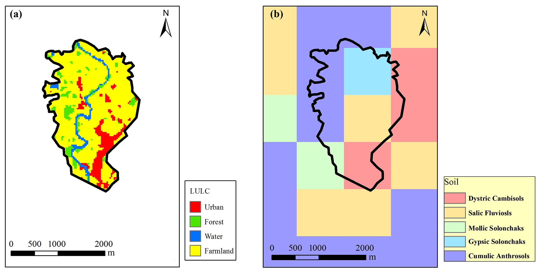
Figure 19 LULC and soil of Helin basin.

The input datasets for the DBCM include the DEM, the LULC (land use and land cover), and the soil type as shown in Figs. 18 and 19. DEM data were obtained from the GDEMV2 database with a spatial resolution of 30 m. The DEM was resampled according to field survey datasets of the channel section in order to obtain fine-resolution topography. There are four main kinds of land use types involves in the Helin basin: urban, forest, farmland, and water. In addition, several soil types with a small proportion have been consolidated into the categories with a large proportion. Soil properties determine the infiltration rate, which further affects the surface runoff. The parameters, such as roughness and soil moisture content, are extracted from the data provided by local administrative sectors. The LULC data are processed by remote sensing interpretation tools using the satellite image. The soil data are processed by the Soil & Water Assessment Tool (SWAT), Soil-Plant-Air-Water (SPAW) model using the Harmonized World Soil Database (HWSD).

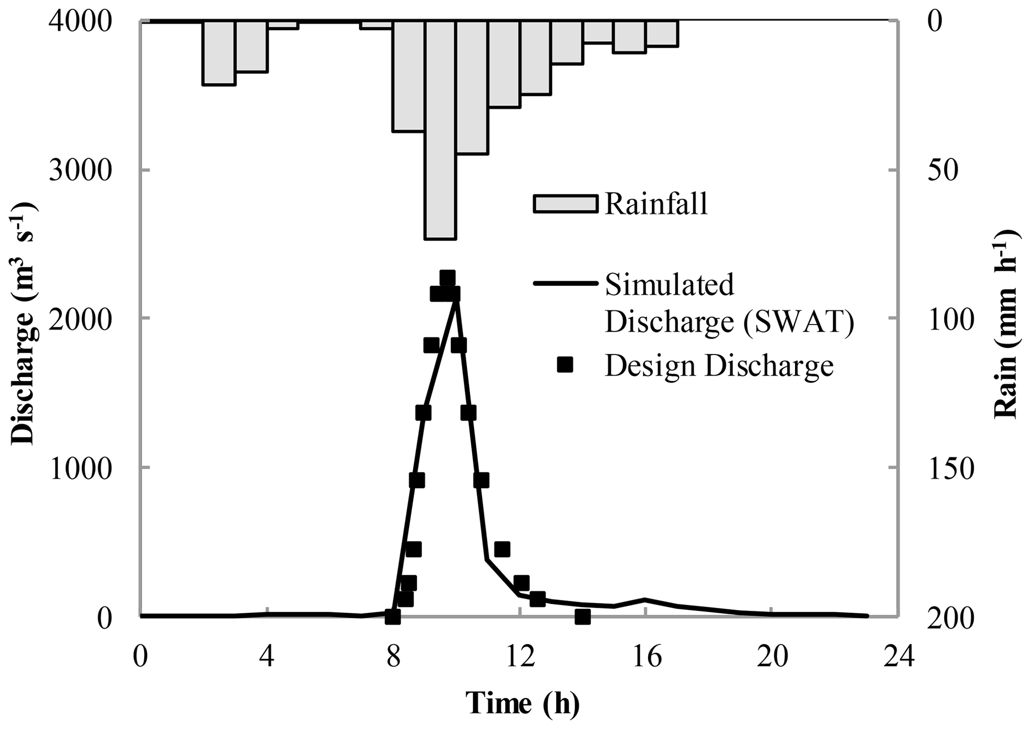
The DBCM was applied to simulate the rainfall–runoff process in Helin Town and was compared with a UCM composed of SWAT (as the hydrologic model). SWAT was calibrated by the design storm and hydrographs (flood return period of 1 %) in the Helin Town outlet. The selected coefficients and parameters of rainfall and flood event are listed in Tables 3 and 4. The calibration results are shown in Fig. 20. It can be seen clearly that the flooding process calculated by the SWAT model is very similar to the design flood, with similar flood peak flow and fluctuation processes. At the beginning of the simulation, because of the soil infiltration, there is no surface runoff, although the rainfall occurs for a short time. However, when the soil saturates, the discharge curve climbs rapidly, which is consistent with the rainfall intensity. The simulation result reflects the storm runoff production process affected by the combination of precipitation process and infiltration process. The hydrographs show good agreement with the design flood, demonstrating that results from SWAT are reliable for the hydrodynamic model. Once calibrated, the hydrographs generated by SWAT at different locations were extracted and applied as inflow boundary conditions for hydrodynamic models. Two simulation scenarios were designed, as shown in Table 2.

Table 2 Simulation scenarios.

Table 3 Rainfall parameters (C_s: coefficient of skewness; C_v: coefficient of variation; P: flood recurrence period). Bold font denotes the values used in the simulation.

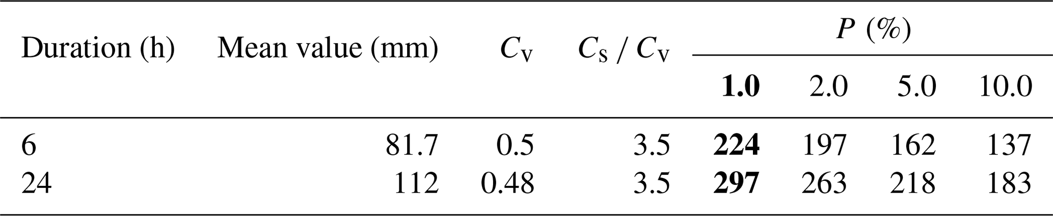
Table 4 Peak discharge at Helin outlet for different flood frequencies. Bold font denotes the values used in the simulation.

Figure 20 Design rain and flood with calculated flow in Helin basin outlet (1 %).

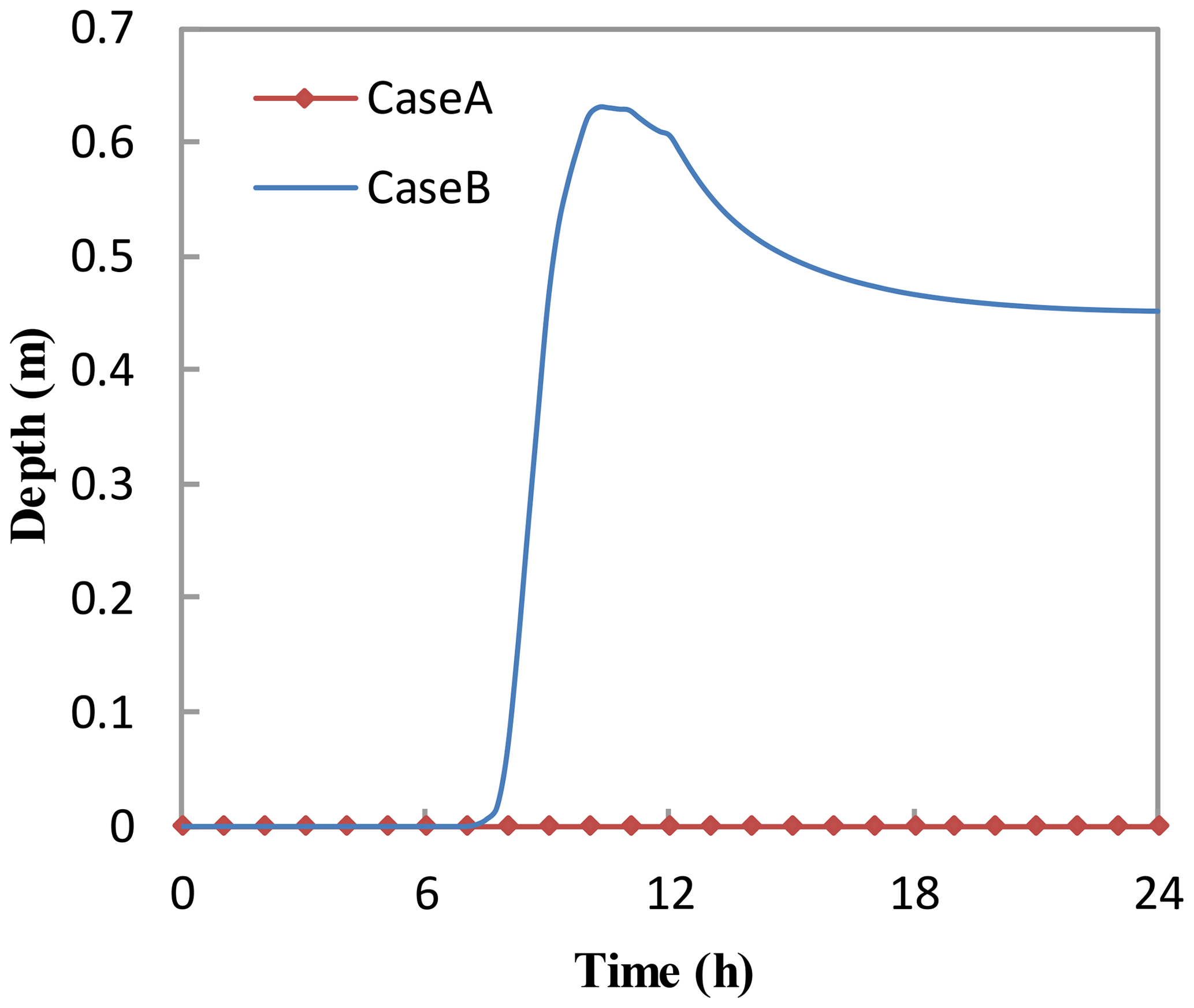
The results obtained in Case A and Case B are compared to investigate the capability of the DBCM. Figure 21 depicts the maximum water depth distribution. The inundation region has expanded significantly in Case B. Not only the lowland areas but also the hillsides have been inundated. Even though Case A adopted the simulated outlet hydrographs larger than those in Case B, the runoff failed to inundate the hillside because of the topographic feature. The red cycle in Fig. 21 indicates the urban area. Water depth was extracted for each case. Due to the lack of measured data, field survey and historical records have to be used as reference data to verify the model outputs. There are several problems involved in the current river topographic conditions: both sides of the river are flat, with a lot of farmland and some villages distributed along the main river. No embankments or bank protection works have been built along the river. All of these problems lead to a low flood control capacity. As local residents recall, in 2017, the flood covered the middle of the trees along the river bank, equivalent to at least 3 m water depth. In terms of the urban area, according to the historic record, a rainstorm in 12 August 1998 caused a flash flood that inundated the local streets and airports with a water depth of 1.0 and 1.4 m respectively. All villages and towns around the Helin Town catchment were submerged with water depth exceeding 0.5 m on average. In Case B, this phenomenon was simulated and it was found that the maximum water depth in urban areas was more than 0.6 m, in accordance with the historic data. But no water emerged in Case A, although the Helin outlet flow is utilized as inflow discharge, greater than that of Case B, as shown in Fig. 22. Referring to local topography, the main reason for this issue is that the urban areas are located in a higher position, between riverbed and hillside; hence the upwelling movement of water in rivers is easily blocked due to local terrain. Nevertheless, the urban area will be submerged by uphill surface flow, even though the river flow has been obstructed. It can be seen that the computed results of Case B by the DBCM are closer to the practical situation.

Figure 21 Comparison of maximum depth: (a) Case A and (b) Case B. The red circle denotes the location of Helin Town (satellite imagery base map was obtained from © Google Earth).

Figure 22 Comparison of water depth variation.

In DBCM, the coupling boundary is time-dependent, and the grid cells on each side solve for different models (whether DWE or SWE). The water depth threshold (0.01 m) is used to distinguish the two models in this case. Flux calculation was only conducted within SWE cells, since there is no need of flux information for DWE cells. As shown in Fig. 24, the rainfall stopped 17 h later, and then the surface flow on the slope gradually decreased. However, a small amount of water is still left within the sloping area where the grid cell information was solved by DWE. Thus, even though the flux calculation has stopped, flow velocity still exists in most of the slope areas. The low-lying area on the northeast corner, due to the obstruction of the terrain, cannot be flooded in Case A. However, using the DBCM, the confluence of the surrounding slope accumulated to the local area and formed a small range of flooded area.

Figure 23 shows the evolution of the coupling boundary of the DBCM in Case B. In the first 8 h, rainfall intensity was small (see Fig. 19), and most of the runoff was infiltrated underground. Thus, the surface flow was determined by SWE with the upstream inflow. After that, rainfall began to increase, and runoff started to generate surface flow using the DWE. The region of SWE continued to extend until the inundation area reached a maximum value. And then the area began to shrink with the recedence of rainfall.

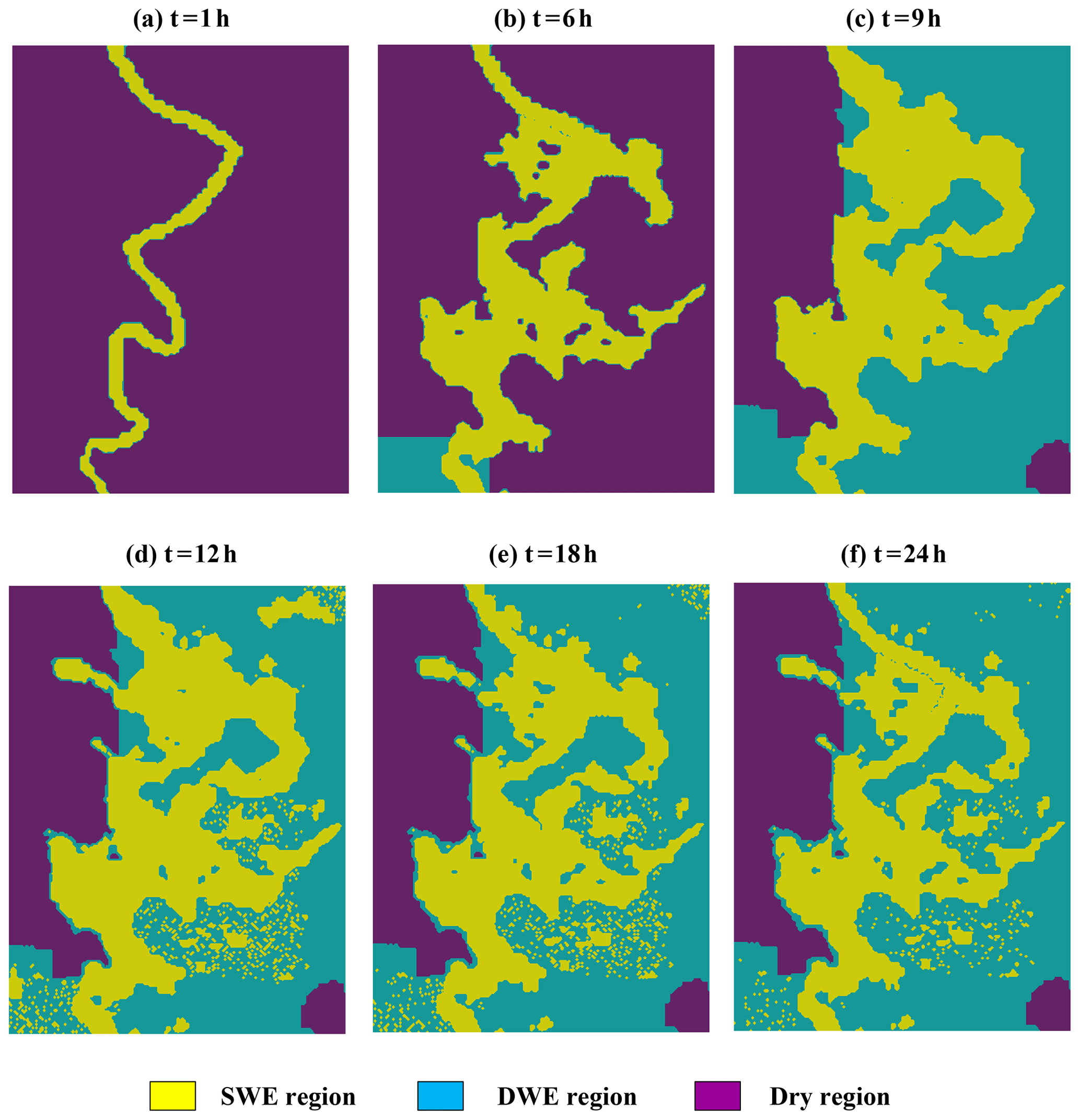
Figure 23 Evolution of coupling boundary.

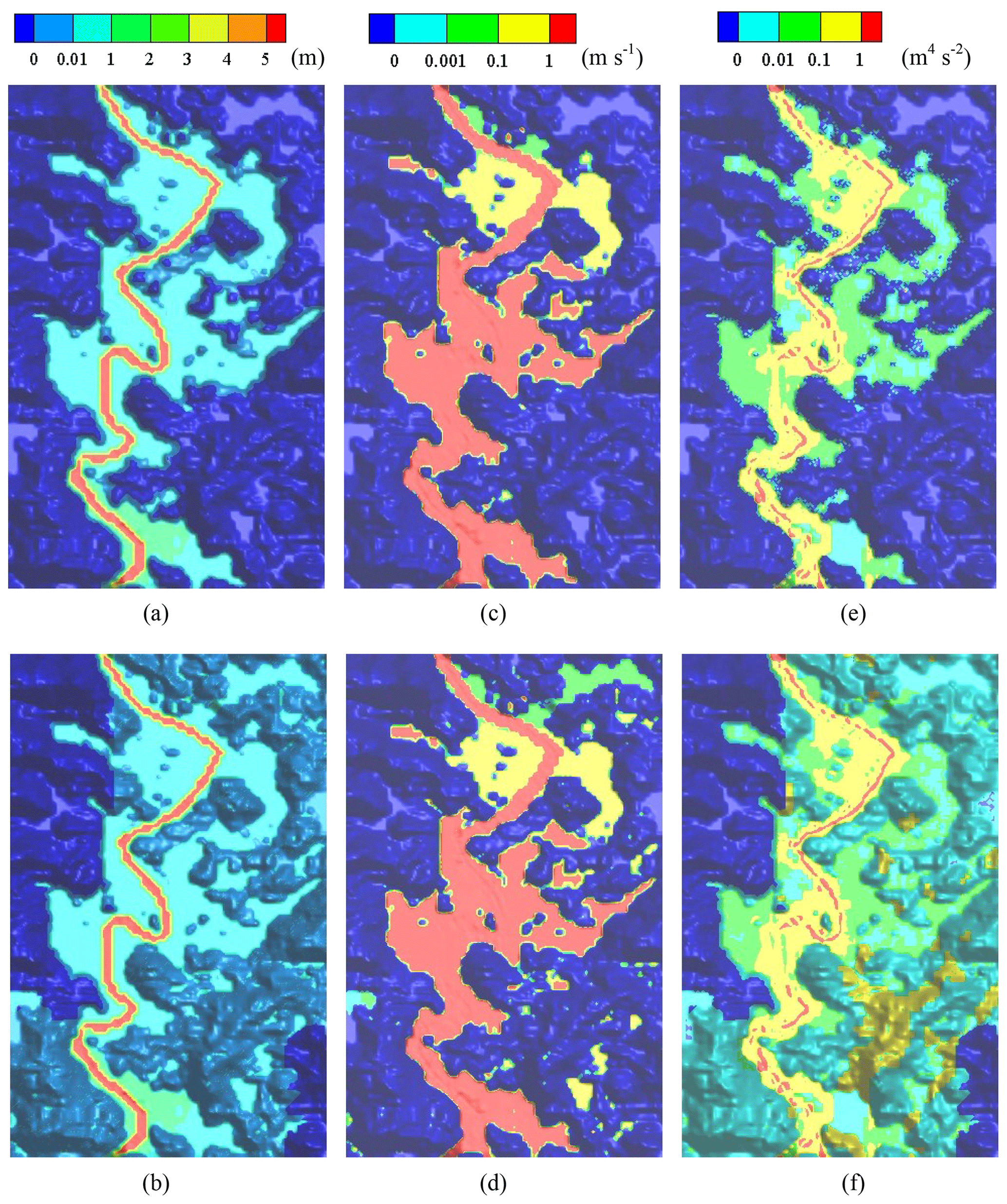
Figure 24 Simulation results at t=17 h. Panels (a) and (b) are water depth (m) for Case A and Case B. Panels (c) and (d) are velocity (m s⁻¹) for Case A and Case B. Panels (e) and (f) are the flux term (m⁴ s⁻2) for Case A and Case B.

5 Conclusions

A dynamic bidirectional coupling model (DBCM) for surface flow inundation simulation has been developed. In the DBCM, the runoff production is depicted by the hydrologic model through the rainfall–runoff process, while the hydrodynamic model is used to simulate the flood propagation processes. The characteristic wave theory is applied to determine the coupling boundary between the hydrologic and hydrodynamic computational domains.

The DBCM can dynamically alter the coupling boundary position to determine the non-inundation and inundation regions, which take into account both mass and momentum exchange on the coupling boundary. The hydrologic and hydrodynamic models are solved simultaneously. The coupling approach in DBCM shows more approximation to the natural physical process of flood formation and propagation, which has the potential to improve the accuracy of flood prediction.

The main advantages of the proposed DBCM are threefold: (1) flow discharge at the coupling boundary is determined based on the characteristic wave theory. Solution of the hydrologic model and hydrodynamic model on each side of the coupling boundary is achieved with characteristic wave analysis and slope gradient analysis, respectively. (2) The discharge obtained on the coupling boundary takes into account both mass and momentum transfer between the hydrologic model and hydrodynamic model, and flow information on both sides of the coupling boundary can be reflected. (3) The coupling boundary is time-dependent, and the computational domain of inundation and non-inundation regions varies according to the flow state throughout the calculation process, which is more aligned with natural rainfall and flood propagation conditions. The benchmark tests show that the DBCM is capable of accurately simulating the hydrologic and hydrodynamic response to rainfall events in various catchments. The DBCM gains a good agreement with the analytical solution and realizes the dynamic switching between the hydrologic and hydrodynamic models in simulating surface flows, which is hardly achieved by former methods. The DBCM also succeeds in predicting the inundation regions in real flood events with more reasonable results when compared to the BCM.

However, the DBCM in the present study only accounts for precipitation and infiltration among the various physical processes of the hydrological cycle. In addition, uniform rainfall station data were adopted in the present DBCM, which limits its application to relatively small-scale catchment simulation. Thus, further study involving other physical processes, such as evapotranspiration, interception, and snow melt, as well as distributed rainfall dataset processing needs to be implemented in the DBCM in order to make it suitable for more general application and complicated case studies or practice.