the Creative Commons Attribution 4.0 License.
the Creative Commons Attribution 4.0 License.
 | 16 Dec 2021
Evaluating landslide response in a seismic and rainfall regime: a case study from the SE Carpathians, Romania
Léna Cauchie
Anne-Sophie Mreyen
Mihai Micu
Hans-Balder Havenith
There have been many studies exploring rainfall-induced slope failures in earthquake-affected terrain. However, studies evaluating the potential effects of both landslide-triggering factors – rainfall and earthquakes – have been infrequent despite rising global landslide mortality risk. The SE Carpathians, which have been subjected to many large historical earthquakes and changing climate thus resulting in frequent landslides, comprise one such region that has been little explored in this context. Therefore, a massive (∼9.1 Mm2) landslide, situated along the river Bâsca Rozilei, in the Vrancea seismic zone, SE Carpathians, is chosen as a case study area to achieve the aforesaid objective (evaluating the effects of both rainfall and earthquakes on landslides) using slope stability evaluation and runout simulation. The present state of the slope reveals a factor of safety in a range of 1.17–1.32 with a static condition displacement of 0.4–4 m that reaches up to 8–60 m under dynamic (earthquake) conditions. The groundwater (GW) effect further decreases the factor of safety and increases the displacement. Ground motion amplification enhances the possibility of slope surface deformation and displacements. The debris flow prediction, implying the excessive rainfall effect, reveals a flow having a 9.0–26.0 m height and 2.1–3.0 m s−1 velocity along the river channel. The predicted extent of potential debris flow is found to follow the trails possibly created by previous debris flow and/or slide events.
- Article
(25428 KB) - Full-text XML
-
Supplement
(851 KB) - BibTeX
- EndNote


Landslides, though a normal process of hillslope erosion, pose socio-economic risk to human life and infrastructure (Gupta et al., 2017; Froude and Petley, 2018; Pollock and Wartman, 2020; Kumar et al., 2021). Despite the rising global landslide mortality risk, effective evaluation of disastrous influences of landslides has been infrequent (Sassa, 2015; Haque et al., 2019; Klimeš et al., 2019). Such evaluation approaches could be regional (susceptibility/hazard/risk/vulnerability) or local (slope stability, runout prediction, monitoring/change-detection mapping) (Fell and Hartford, 1997; Van Westen et al., 2006; Margottini et al., 2013; Hungr, 2018). However, effectiveness in such approaches cannot be justified until the main landslide-triggering factors – rainfall and earthquakes – are evaluated together. Despite the numerous case studies of rainfall-induced slope failures in earthquake-affected terrain (Lin et al., 2006; Helmstetter and Garambois, 2010; Tang et al., 2011; Durand et al., 2018; Bontemps et al., 2020), studies predicting the potential effects of both factors have been relatively rare. The necessity of such studies becomes more critical in view of an annual average of >4000 landslide-related deaths worldwide in the last decade (Pollock and Wartman, 2020).
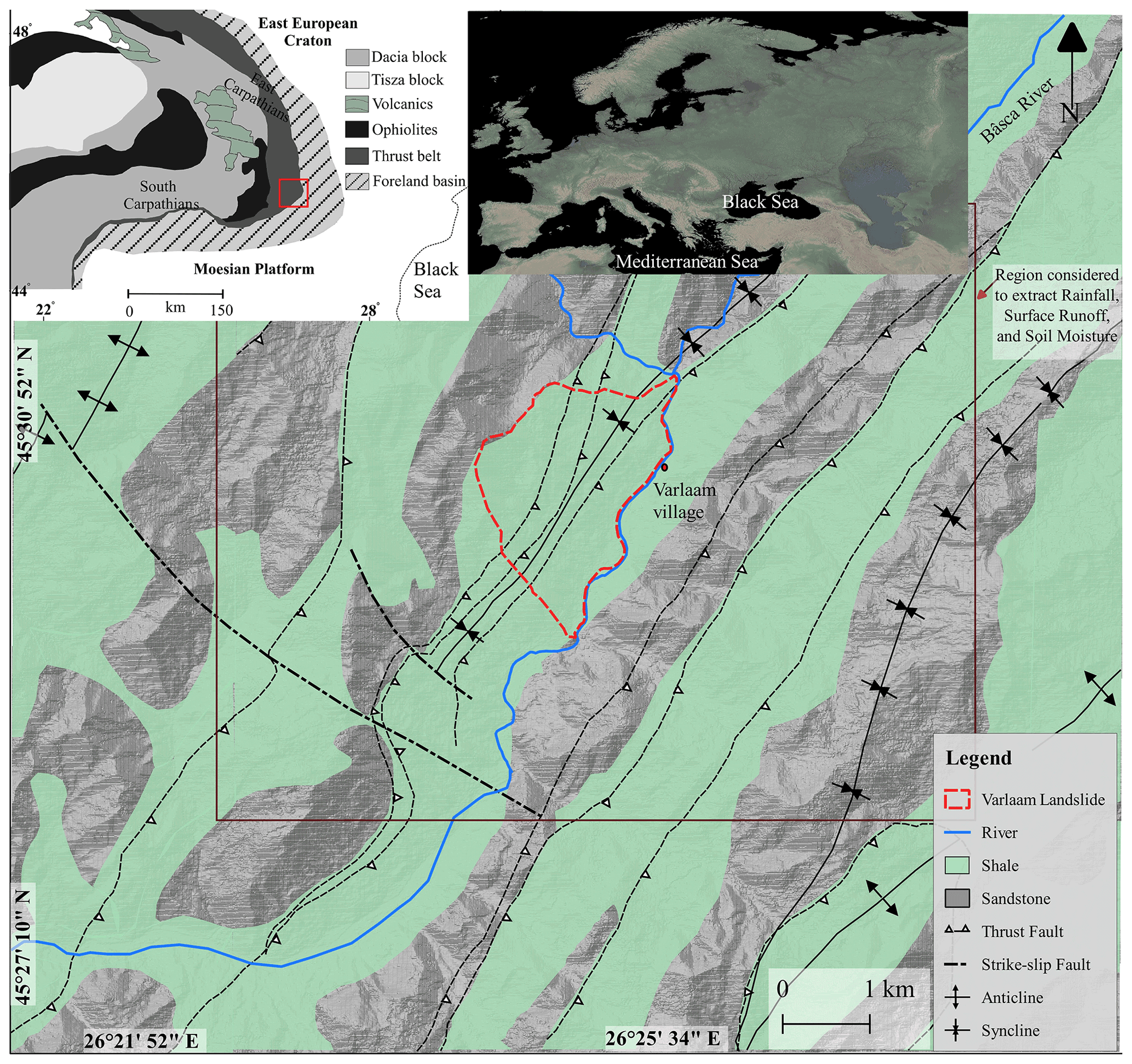
Figure 1Study area. Inset (a) (source: NOAA NCEI, USA) and (b) (after Ustaszewski et al., 2008) highlight the position of the study area. Geological setting is based on Murgeanu et al. (1965), Tischler et al. (2008), and Pospíšil et al. (2012).
Owing to the capability to represent the progressive deformation in the slope under various loading conditions, numerical-modeling-based analysis can be considered one of the few approaches for effective evaluation of slope instability and associated risk (Jing, 2003; Fenton and Griffiths, 2008). Though the continuum-modeling-based approaches have been common for local-scale evaluation of hillslope response (Griffiths and Lane, 1999; Jamir et al., 2017; Kumar et al., 2018, 2021), their limitations in estimating large strain, particularly during dynamic analysis, make the discontinuum modeling a better option (Havenith et al., 2003; Bhasin and Kaynia, 2004). Apart from the stability evaluation, prediction of potential runout during the slope failure constitutes a principal risk evaluation approach (Hungr et al., 1984; Hutter et al., 1994; Rickenmann and Scheidl, 2013). Among different types of landslide, debris flows have been shown to have the maximum outreach, cause more fatalities, and cause secondary effects like river damming and subsequent outburst flooding (Jakob et al., 2005; Ding et al., 2020; Kumar et al., 2021). Among different runout prediction approaches, dynamic-model-based Rapid Mass Movement Simulation (RAMMS) (Christen et al., 2010), FLO-2D (O'Brien et al., 1993), and MassMov2D (Beguería et al., 2009) have been the more useful ones (Rickenmann and Scheidl, 2013; Kumar et al., 2021).
In view of these understandings, the present study aimed to infer the potential response of a landslide slope under seismic and extreme rainfall conditions using stability evaluation and runout simulation. Such simulations/modeling outputs depend upon certain input parameters and criteria, the values of which might be affected by uncertainties due to nonlinear behavior of material. Therefore, a parametric analysis is also performed to evaluate uncertainty. In order to achieve the aforementioned objectives, a massive (∼9.1 Mm2) landslide in the Vrancea seismic zone, SE Carpathians, is chosen as a case study area. The region has been subjected to frequent earthquakes and relatively wet climatic conditions that induce frequent landslides and related socio-economic losses (Micu et al., 2013, 2016; Micu, 2019; Mreyen et al., 2021).
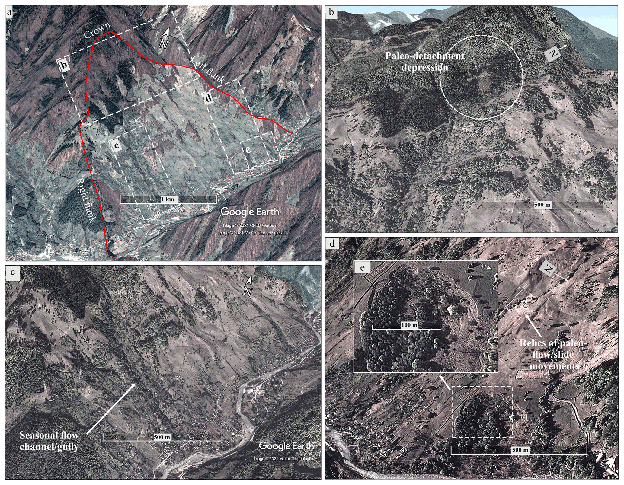
Figure 2Landslide features. (a) Landslide marked with different features. (b) Crown portion. (c) Right flank. (d) Left flank. (e) Signs of failure in the flow deposits. Image source: © Google Earth.
2.1 Geological setting and geomorphology
The landslide is situated at 45∘30′23′′ N, 26∘25′05′′ E along the river Bâsca Rozilei in the SE Carpathians, Romania (Fig. 1). The earliest record of this landslide is mentioned in the geological map by Murgeanu et al. (1965). Unfortunately, no previous record and/or dating is available at present. The slope is composed of shale belonging to the Miocene thrust belt that separates the external foredeep in the north, east, and southeast from the inner Carpathian mountain ranges. Thrust faults, strike-slip faults, and folds traverse the region in and around the vicinity of landslide slope. The origin of these structural features has been related to the Eocene–Miocene collision of the ALCAPA and Tisza–Dacia plates against the Bohemian and Moesian promontories that gave rise to the Carpathians (Tischler et al., 2008). The SE part of the Carpathians, however, is still uplifting at a rate of 3–8 mm yr−1 due to the foreland coupling of the converging plates (Pospíšil and Hipmanova, 2012; Maţenco, 2017).
The landslide toe along the river hosts the village of Varlaam (Figs. 1 and 2a). The landslide has a slope gradient ranging between 15–20∘ and encompasses an area of ∼9.1 Mm2. The landslide-affected area is covered by shrubs and scattered trees towards its flanks and with grasslands in the inner parts, mainly used as pastures and hayfields. The landslide crown region has a depression that might be a surficial imprint of the paleo-detachment (or depletion zone) (Fig. 2b). Near the right (or southern) flank, a seasonal flow channel (or gully) emerges near the paleo-detachment depression and finally merges at the river channel (Fig. 2c). Near the left (or northern) flank, the slope surface comprises flow relics, possibly of paleo-debris flow and/or slide events (Fig. 2d), as also inferred from loose/unconsolidated deposit at the slope toe (Fig. 2e). This flow deposit is noted to develop 100–150 m wide minor scarps (Fig. 2e). Such scarps may further grow and result in the debris flows during extreme rainfall and/or earthquake events and hence pose a risk to the nearby human settlement.
2.2 Rainfall and earthquake regime
The study area is subjected to an increasing rainfall trend (Fig. 3a). The average monthly rainfall was 50±1.6 (SE) mm during the years 1982–2019 and has increased in recent decades (2000–2019) to 53±2.3 (SE) mm (Fig. 3b). Monthly rainfall patterns further reveal higher rainfall in the months of May, June, and July (Fig. 3c). Such enhanced summer (June–July) rainfall has been related to the existing positive phase of the North Atlantic Oscillation (NAO) index that allows the strengthening of continental climate, Mediterranean retrogressive cyclones, and the Siberian High in central and southern Europe (Constantin et al., 2007; Magyari et al., 2013; Obreht et al., 2016).
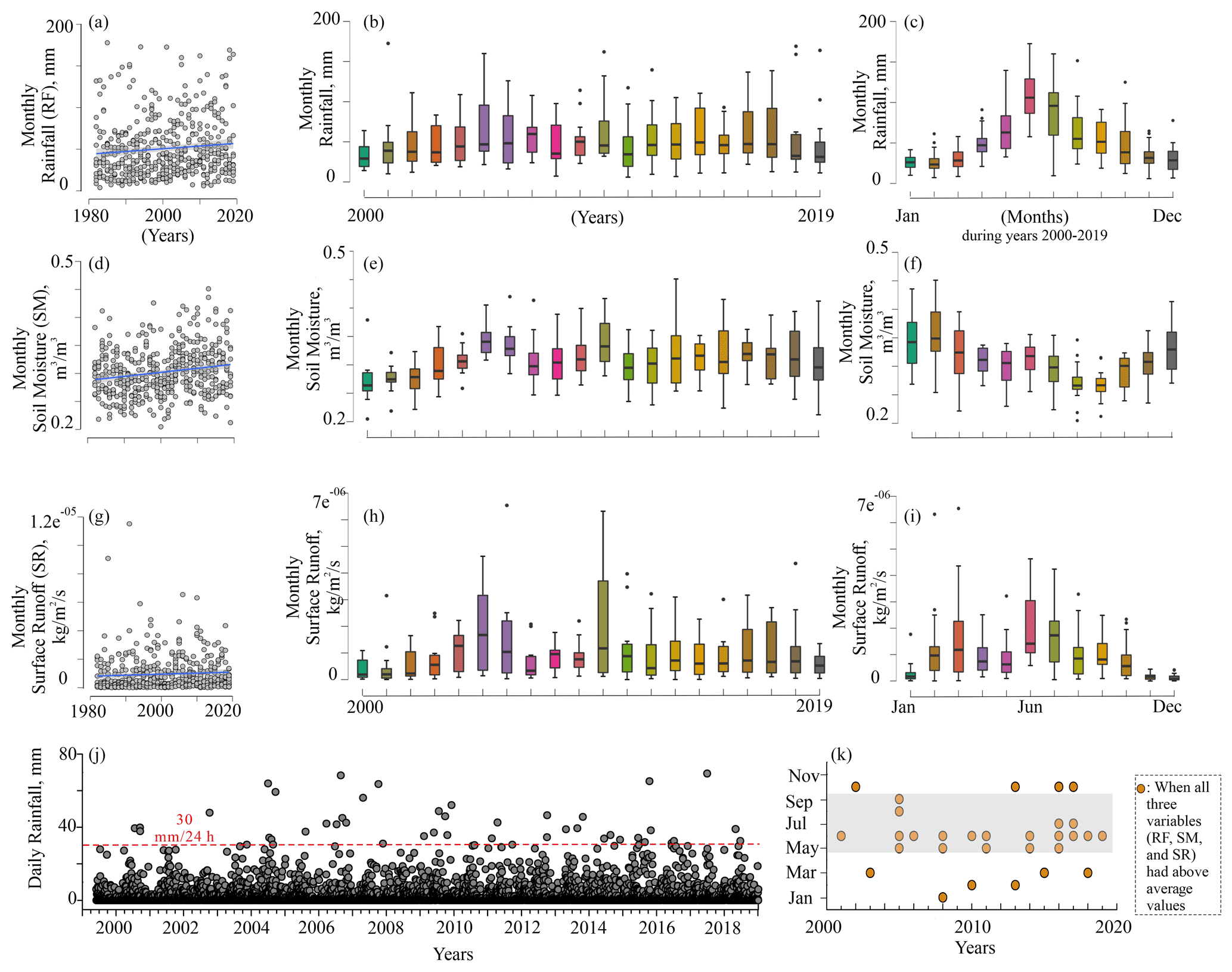
Figure 3Rainfall (RF), soil moisture (SM), and surface runoff (RF) pattern. The region from which these parameters are extracted is highlighted in Fig. 1. Dataset (except j) source: FLDAS_NOAH01_C_GL_M model (McNally, 2018). Spatial resolution of dataset: 0.1∘ (∼10 km). Data source of (j): GPM IMERG Final Precipitation (Huffman et al., 2019). Spatial resolution of dataset: 0.1∘. The rainfall data in (j) are available only from 1 June 2000. The SM and SR data are not available at a daily scale for the study area. The blue line (in a, d, g) indicates linear regression, and the shaded region around it refers to the 95% confidence interval. Dots in box plots refer to outliers. The red line in (j) refers to extreme rainfall (30 mm d−1). The grey-shaded region in (k) refers to those months that witnessed above-average values of RF, SM, and SR.
Apart from the rainfall, soil moisture and surface runoff also show increasing trends during the years 1982–2019 (Fig. 3d and g). Though the average monthly soil moisture and surface runoff have also increased in recent decades, their trends do not follow rainfall entirely (Fig. 3e and h). This occurs due to the fact that the temporal coexistence of rainfall, surface runoff, and soil moisture depends upon the rainfall threshold and soil conditions (antecedent soil moisture). Further, the surface runoff (water, from precipitation that flows over the land surface) correlates relatively well with the rainfall, unlike the soil moisture, which retains part of the rainfall before achieving saturation and hence does not correlate well (Fig. S1 in the Supplement). This difference in correlation is further visible in the monthly pattern (Fig. 3f and i). It is of note that the surface runoff and soil moisture data are based on the FLDAS (Famine Early Warning Systems Network Land Data Assimilation System) model (McNally, 2018). This utilizes precipitation datasets and analyses like CHIRPS (Climate Hazards Group InfraRed Precipitation with Station data) and MERRA-2 (Modern-Era Retrospective analysis for Research and Applications, Version 2) along with land cover data to derive variables like soil moisture and surface runoff.
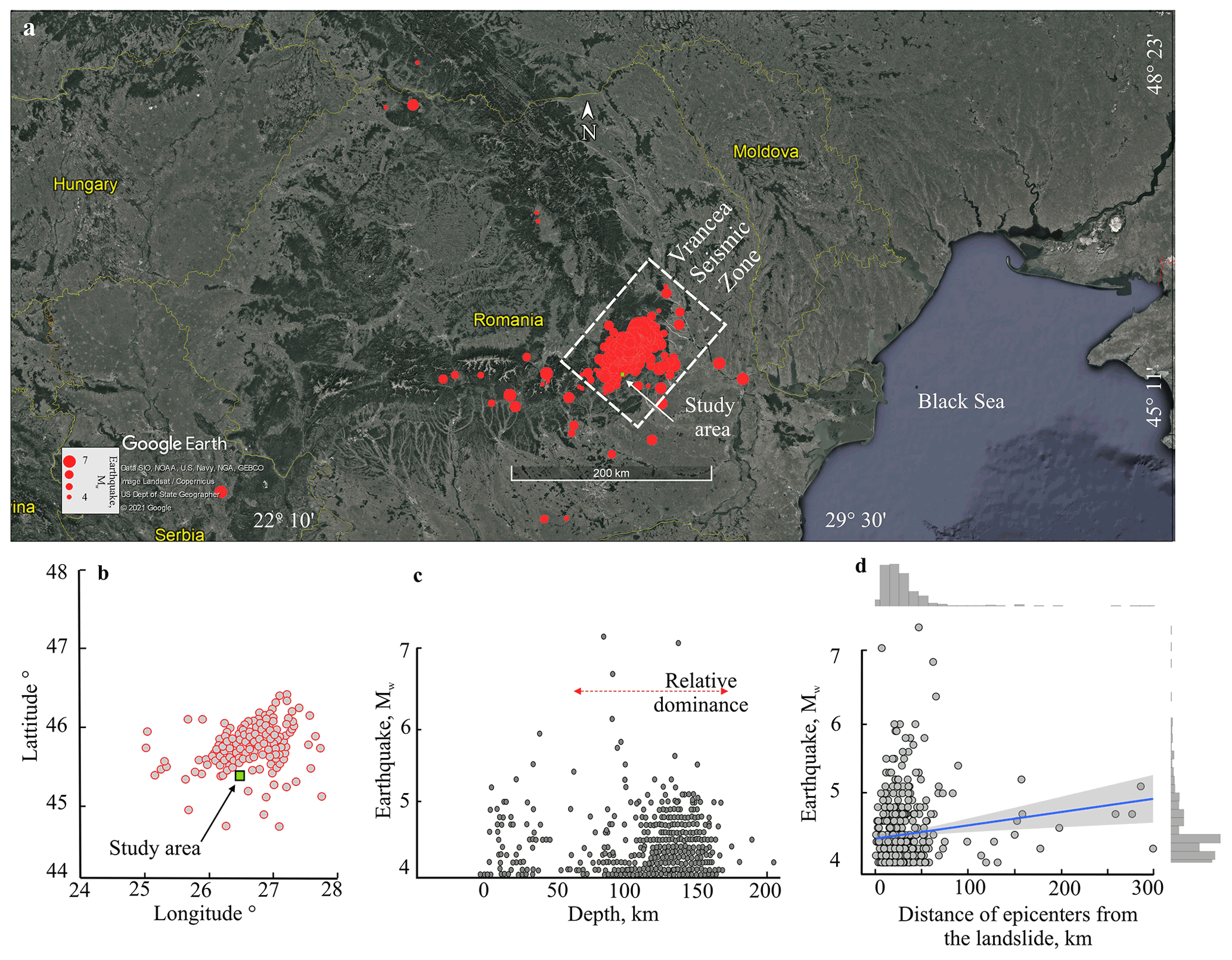
Figure 4Earthquake pattern. (a, b) Position of study area. (c) Depth and earthquake magnitude. (d) Distance of epicenters from landslide and earthquake magnitude. The blue line (in d) indicates linear regression, and the shaded region around it refers to the 95 % confidence interval. Data source: National Institute for Earth Physics, Romania.
Further, the daily rainfall data of the years 2000–2019 revealed 48 extreme rainfall events (Fig. 3j). “Extreme” rainfall pertains to >30 mm d−1 in the region on the basis of previous studies exploring the rainfall variability (Apostol, 2008; Croitoru et al., 2016). Out of these 48 events, 28 events occurred in the last decade, particularly in the years 2005, 2007, 2010, and 2016. The debris flows and flash floods in the region in the years 2005 and 2010 (Micu et al., 2013; Grecu et al., 2017) can be related to these extreme rainfall events in the region. The years 2005 and 2010 had relatively high precipitation due to synoptic conditions that involved pressure lows and front systems moving along a SE–NW trajectory from the Mediterranean Sea and Black Sea towards central Europe and in a west-to-east direction from the Atlantic Ocean to eastern Europe. These trajectories led to severe flood and slope failure events in different parts of central and eastern Europe (Mihailovici et al., 2006; Micu et al., 2013; Grecu et al., 2017). The influence of these trajectories is also visible in the regional rainfall pattern (Fig. S2), where years 2005 and 2010 have higher rainfalls. Though the years 2007 and 2016 also had many extreme rainfall events, these years did not have as high surface runoff as years 2005 and 2010 (Fig. 3h). Notably, many conceptual and physically based models have been proposed relating the initiation of debris flow to surface runoff conditions (Simoni et al., 2020).
Further, the temporal pattern of higher values (above average) of rainfall, surface runoff, and soil moisture revealed that May–September months dominate the trend, having the majority of the events when all three variables had extremes (i.e., above average) (Fig. 3k). These above-average values refer to the monthly scale. The temporal overlapping of these variables further justifies the occurrence of debris flows and flash floods in this region in the last decade and possibility of more such events in the near future (Micu et al., 2013; Ilinca, 2014; Grecu et al., 2017; Micu, 2019).
Apart from the temporally enhanced rainfall, surface runoff, and soil moisture, the study area is also subjected to frequent earthquakes owing to its position in the Vrancea seismic zone, which is one of the most active seismic zones in Europe (Fig. 4a and b). This region has received ∼469 earthquakes (Mw≥4) during the years 1960–2019. The earthquake event cluster represents a NE–SW trend (Fig. 4b). About 75 % of the total earthquake events occurred in a depth range of 60–180 km (sub-crustal depth), and four out of five events having a magnitude ≥ 6 occurred within 60–100 km depth (Fig. 4c). The relative dominance of M≥6 earthquakes in this depth range has been related to the reverse faulting mechanism in this depth range (Radulian et al., 2007; Petrescu et al., 2019). The possible explanation of the pattern of earthquakes has been divided into the following two categories: (1) it might be associated with a descending relic ocean lithosphere beneath the bending zone of the SE Carpathians or (2) it might be associated with a continental lithosphere that was delaminated after the collision (Bokelmann and Rodler, 2014; Petrescu et al., 2019).
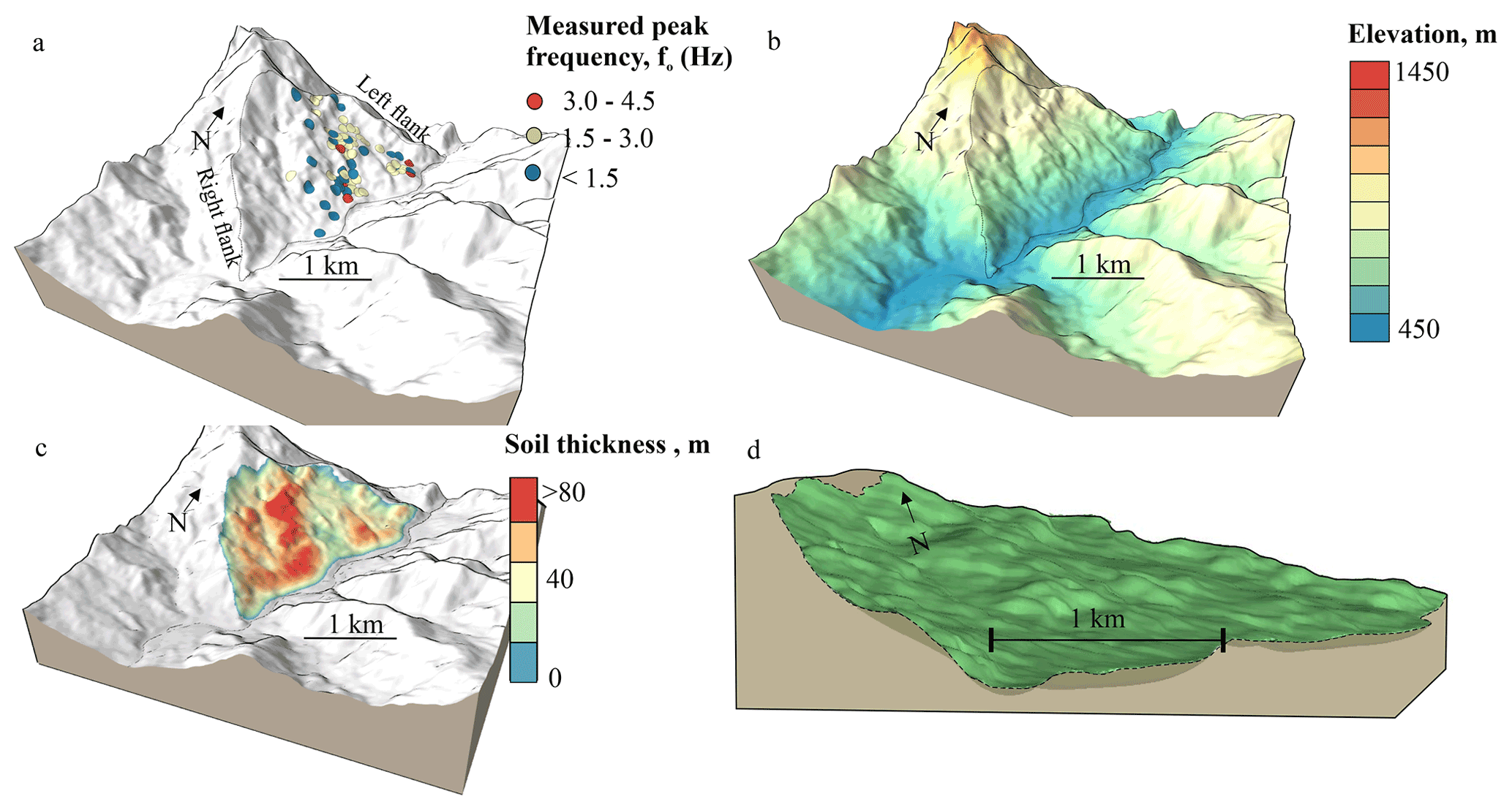
Figure 5Landslide model construction. (a) Measured peak frequency distribution. Based on Cauchie et al. (2019). (b) Digital elevation model. (c) Soil (or debris) thickness pattern in the landslide. (d) Cross-sectional view of landslide model.
Though the majority of earthquakes have their magnitude smaller than 5 and quite deep (mostly between 60 and 180 km), their epicenters are situated within 50 km of the study area (Fig. 4d). Such intermediate to deep earthquakes in the Vrancea region (study area) have triggered landslides as far as 250–300 km from their epicenters (Havenith et al., 2016). Further, any major future earthquake might have ground effects in a much larger area (150 000 km2), possibly causing more landslides (Havenith et al., 2016). The regional distribution of the annual rainfall and earthquakes around the study area is also shown in Fig. S3.
In order to evaluate the landslide response under seismic and extreme rainfall conditions, our approach involved dynamic slope stability analysis and runout simulation, respectively. Both the techniques required a landslide model that was constructed using field-based ambient noise analysis, empirical equations/values, a digital elevation model, and geological modeling software. Details are as follows.
3.1 Debris (or loose material) depth estimation
We analyzed seismic ambient noise at 56 measurement points to estimate the depth of impedance contrasts. The equipment was composed of seven Güralp CMG-6TD 30 s velocimeters, one Lennartz 5 s velocimeter, and one CityShark II velocimeter. The technique aims at estimating the site resonance frequency by computing the spectral ratio between horizontal (NS, EW) and vertical components (Nakamura, 2009). Under particular geological conditions where impedance contrast exists at depth, as representative of a loose/soft material overlying bedrock, the resulting horizontal-to-vertical spectral ratio (HVSR) curve presents a peak in correspondence of the site resonance frequency (fo). Figure 5a represents the location of the inferred fo in a range of <1.5–4.5 Hz. Lower frequencies, generally implying higher thickness of loose material, are noted in the central part and near the right flank.
The thickness (h) of the loose/soft material is consecutively estimated using the shear-wave velocity (Vs) and resonance frequency (fo) in the following equation (Murphy et al., 1971; Ibs-von Seht and Wohlenberg, 1999):
In view of the similar litho-tectonic conditions and spatial proximity, the shear-wave velocity (Vs) values in the present study are based on Mreyen et al. (2021). For the loose overburden (soil) and rock mass, the Vs values are taken as ∼400 and ∼900 m s−1, respectively.
The thickness of the loose material (inferred from the HVSR and Vs) at different measurement locations was later imported into Leapfrog Geo software (v5.1) along with the surface morphology (Fig. 5b). The surface morphology with a spatial resolution of ∼12 m is based on the TanDEM-X (TerraSAR-X add-on for Digital Elevation Measurement) digital elevation model. The surface morphology and depth information of loose material were integrated using Leapfrog Geo (v5) to construct a continuous soil thickness layer and hence a 3D model of the landslide (Fig. 5c and d). This model was later used to extract the 2D slope sections (CS-1, CS-2, CS-3, and CS-4) for the slope stability evaluation (Sect. 3.2) and runout simulation (Sect. 3.3).

Figure 6Model configuration for the slope stability analysis. (a) Landslide model. The location of the different cross sections used in the UDEC models are marked by red lines. (b–e) Configuration of the sections: CS-1 to CS-4.
3.2 Slope stability evaluation
The 2D slope sections (CS-1, CS-2, CS-3, and CS-4), shown in Fig. 6a, were used to determine the hillslope response under static (gravity) and dynamic (seismic) conditions by performing slope stability analysis in UDEC (2014) software. Each slope section comprises loose overburden (soil) over rock mass and an interface joint separating these blocks (Fig. 6b–e).
Under static conditions, the factor of safety of the slope and potential material displacement are determined, whereas under dynamic conditions, the potential material displacement, peak ground acceleration (PGA), and spectral ratio are evaluated. The factor of safety is determined using a shear strength reduction approach (Matsui and San, 1992; Griffiths and Lane, 1999). The potential material displacement under static conditions refers to displacements after the model has reached static equilibrium under gravity load. The spectral ratios are used to understand the response of the medium to the input signal by comparing the signals obtained in the monitoring points at the surface with the signal at the monitoring point at depth (base) (McCowan and Lacoss, 1978).
For the PGA and spectral ratio, material models are considered elastic, whereas for the factor of safety and material displacement (static/dynamic) calculations, elasto-plastic models are considered. The elastic material model involved modulus (elastic/shear/bulk) values of the rock mass and soil. In elasto-plastic conditions, modified Hoek–Brown (MHB) plasticity criteria (Hoek et al., 2002) and Mohr–Coulomb (M–C) plasticity criteria (Coulomb, 1776; Mohr, 1914) are used for the rock mass and soil, respectively. The joint plane is assigned Coulomb slip criteria (Coulomb, 1776) in both elastic and plastic conditions. For dynamic analysis, two different signals, i.e., the Ricker wavelet (Ricker, 1943) and a signal record of the 1976 Friuli earthquake, are used (Fig. 8).
The Ricker wavelet, a theoretical waveform, provides the advantage of being a relatively short signal marked by energy distributed over a range of frequencies. Therefore, the PGA and spectral ratios are evaluated using the Ricker wavelet to understand the ground motion amplification on the landslide surface. Notably, in many studies such ground motion amplification is found to enhance the slope instability (Lenti and Martino, 2012; Del Gaudio et al., 2019). The Ricker wavelet has been used in several studies owing to its reliable representation of seismic waves propagating through the viscoelastic homogeneous media (Gholamy and Kreinovich, 2014). Further, the displacement is determined using both dynamic signals (Ricker wavelet and Friuli earthquake, 1976) to evaluate the difference.
Soil and rock mass blocks in the cross sections (CS-1 to CS-4) were discretized into finite-difference zones of 6 and 20 m size, respectively, according to the following relation (Kuhlemeyer and Lysmer, 1973):
Here, Δl is zone size and λ is the wavelength associated with the dominant frequency. λ can be determined using , where C is the speed of wave propagation associated with the fundamental frequency (f). For the C (or shear-wave velocity) of soil and rock mass, we used 400 and 900 m s−1, respectively (Sect. 3.1). f = 2.0–4.5 Hz was considered a central frequency range. The lateral boundaries in all four slope sections (or models) were considered free-field boundaries owing to the near-surface position of the hillslope (Fig. 6). A stress-boundary condition (Joyner and Chen, 1975; UDEC, 2014) was applied at the base in which the horizontal direction is considered viscous, whereas the vertical direction is kept free. This stress-boundary condition converts seismic input from velocity waves to stress waves. To approximate the natural attenuation in the models during the seismic loading, Rayleigh damping with a 0.02 damping ratio (i.e., 2 % fraction of critical damping) and 2.5 Hz central frequency was used with both the mass and the stiffness damping. Though most of the soil types and rock mass possess the damping in the 2 %–5 % fraction of the critical damping (Biggs, 1964), plasticity models (M–C criteria) and the presence of joints result in further energy loss (UDEC, 2014). Therefore, the damping ratio was kept at the lower level of the suggested range.
Since the area is subjected to temporally enhanced rainfall (Sect. 2.2) and some studies have noted the percolation of rainfall water in the loose material resulting in the groundwater (GW) level increase and subsequent slope instability (Van Asch et al., 1999; Liang, 2020), the effect of the GW is also explored. To simulate the GW effect, coupled hydraulic (fluid-flow)–mechanical analysis was used in which mechanical deformation and joint fluid pressure affect each other as analysis progresses. Further, the model was brought to static equilibrium before performing factor of safety (FS) calculations. Notably, FS calculations were also performed under mechanical stress only (without GW). Steady-state (water table) fluid-flow analysis was used to simulate fluid flow. The GW is included in static as well as in dynamic analysis in plasticity conditions. UDEC allows the GW simulation through the joints as per the parallel plate model (Witherspoon et al., 1980). The parameters and their values used in the static and dynamic analysis are given in Table 1.
Table 1Input parameters used in the slope stability analysis.
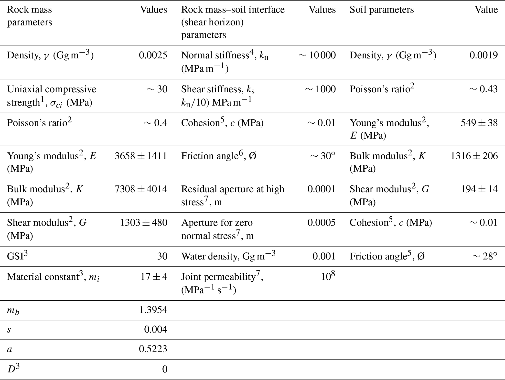
1 It was inferred from the empirical equation of Kahraman (2001) using the VS and VP data of Mreyen et al. (2021). 2 These values were inferred from the empirical equations of McDowell (1990) using the P- and S-wave velocity of Mreyen et al. (2021). 3 Based on Hoek and Brown (1997) and field observation. 4 It was inferred from the empirical equations of Barton (1972) and Hoek and Diederichs (2006) using the elastic modulus of rock and approximated spacing of joint sets of ∼5–10 cm. This spacing was assumed in view of the highly sheared nature of rock mass. 5 Based on Bednarczyk (2018) and Peranić et al. (2020) due to similar litho-tectonic conditions. 6 Based on Barton and Choubey (1977). 7 Based on UDEC (2014).
A parametric analysis was also performed to justify the selection of values of different input parameters by evaluating the change in the output parameters in response to the change in different input parameters. Out of four slope sections, CS-2 and CS-3 were chosen to perform the parametric analysis in view of their central position in the landslide and the heterogeneity in soil thickness and topography (Fig. 6c and d). In order to understand the effect of the GW level change, two GW levels were considered in the CS-2 and CS-3 sections. Since UDEC simulates the fluid flow through a joint aperture, the GW level change is manifested by different heights (h1, h2) of the GW at the joint. Here, the difference in h1 and h2, i.e., Δh, is 10 m (Fig. 6d). Among the different input parameters listed in Table 1, the angle of internal friction of soil, joint friction angle, groundwater head, and elastic modulus were used for the parametric analysis. It is of note that the bulk and shear modulus were also changed along with elastic modulus because all three modulus parameters are interrelated (McDowell, 1990). Though each parameter might have a certain effect on the output, these four have been noted to affect the factor of safety and displacement more (Kumar et al., 2021).
3.3 Runout simulation
The hillslopes affected by the seismic shaking have also been noted to be more prone to rainfall-induced slope failures, particularly in the form of debris flows (Shieh et al., 2009; Tang et al., 2011). Such debris flows can be initiated by either increased pore pressure or runoff involving entrainment (Godt and Coe, 2007). Thus, the increased frequencies of the extreme rainfall, soil moisture, surface runoff, and recent debris flows events in the region (Sect. 2.2) escalate the possibility of debris flow in the Varlaam landslide.
To ascertain the outreach of such potential debris flow during an extreme rainfall event, Voellmy–Salm (Voellmy, 1955; Salm, 1993) fluid-flow continuum-model-based Rapid Mass Movement Simulation (RAMMS) software was used. RAMMS divides the frictional resistance into a dry-Coulomb-type friction (μ) and viscous–turbulent friction (ξ) (Christen et al., 2010). The frictional resistance S (Pa) is thus
where N=ρhgcos (ψ) is the normal stress on the running surface, ρ is density, g is gravitational acceleration, ψ is the slope angle, h is flow height, and u is (ux,uy) consisting of the flow velocity in the x and y directions. A detailed description of the governing equations is presented in the Supplement.
Generally, the values for the μ and ξ parameters are achieved using the reconstruction of real events through simulation and subsequent comparison between dimensional characteristics of real and simulated events. However, the toe of Varlaam landslide merges with the river floor, and hence there is an uncertainty in the reconstruction of the volume of previous flow events that has been washed away by the river. Therefore, μ and ξ are taken in view of the topography of the landslide slope and runout path, landslide material, and previous studies/models (Hürlimann et al., 2008; Rickenmann and Scheidl, 2013; RAMMS v1.7.0). In this study, the maximum allowable friction (μ), i.e., μ=0.4 (or ϕ=21.8∘), was used with the turbulence (ξ) of 250 m s−1 (Table 2). Different depths were considered block release depths in view of uncertainties to ascertain the exact depth of loose material that will be eroded/entrained during the debris flow. Though the landslide surface has some relics of flow channels near the left flank (Fig. 2d and e), the data pertaining to the spatial–temporal pattern of discharge at these flow channel/gullies were not available. Therefore, the release area is chosen as block release because it has been more appropriate when the flow path (e.g., gully) and its possible discharge on the slope are uncertain (RAMMS v1.7.0). The runout stopping criterion is based on the momentum threshold, which was considered 5 % of moving mass. A sensitivity analysis is also performed to evaluate the possible influence of frictional parameters on the debris flow characteristics. Further, in order to understand the influence of river channel morphology on the debris flow characteristics, their interrelationship is also sought.
Table 2Input parameters used in the runout simulation.
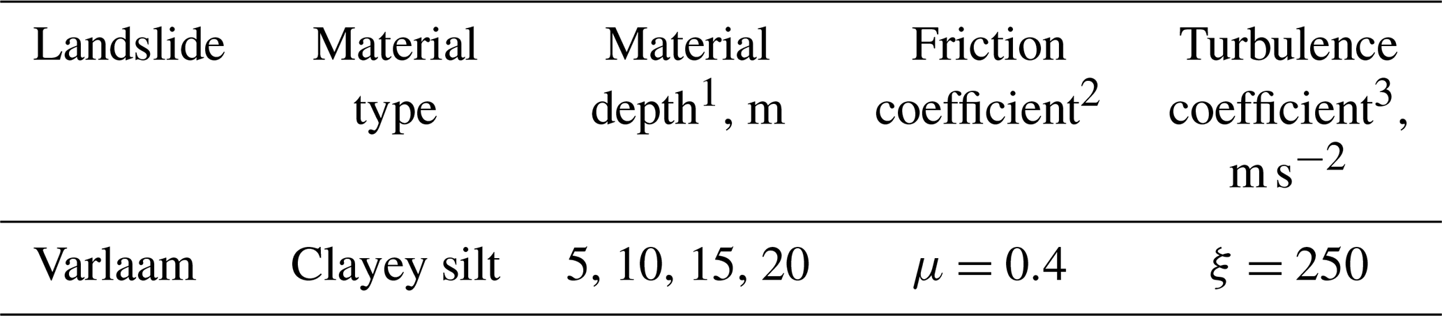
1 Considering the fact that during slope failure, irrespective of the type of trigger, the entire loose material might not slide down, the depth is taken as a variable. 2 In order to keep the results of a conservative nature, we have taken a maximum allowable friction, i.e., μ=0.4 (Hungr et al., 1984; RAMMS v1.7.0). This case is considered to understand the potential impacts of debris flow even after the maximum friction. 3 This range is used in view of the type of loose material, i.e., cohesive (RAMMS v1.7.0).
4.1 Slope stability evaluation
4.1.1 Factor of safety (FS) and displacement
The FS of the slope varies in a range of 1.17–1.32 that decreases further to 1.09–1.29 under groundwater (GW) conditions (Fig. 8). In both cases, the CS-2 model attains the lowest FS, implying more instability. The displacement in loose material was obtained in static, static with fluid (GW), dynamic, and dynamic with fluid (GW) conditions. Under the static conditions, displacement ranges between 0.4–4.0 m, which increases to 0.68–18 m under the GW conditions with its minimum at CS-1 and maximum at CS-2 (Fig. 8). Under dynamic conditions, displacement ranges from 8–60 m and further increases to 7.5–62 m by combining dynamic with GW conditions. Similarly to the static conditions, the minimum displacement is noted at CS-1, whereas the maximum is at CS-2. Further, in all sections (CS-1 to CS-4), displacement accumulated mostly at the upper part of the debris layer (i.e., landslide crown) or at the steepest portion of the slope surface. This spatial affinity of displacement and a steep gradient is caused by the influence of topography on the material displacement (Kumar et al., 2021). Notably, this dynamic displacement pattern pertains to the Friuli earthquake signal (Fig. 7c and d). A comparison of the static and dynamic displacement (caused by the Friuli earthquake signal and Ricker wavelet) is presented in Fig. 9.
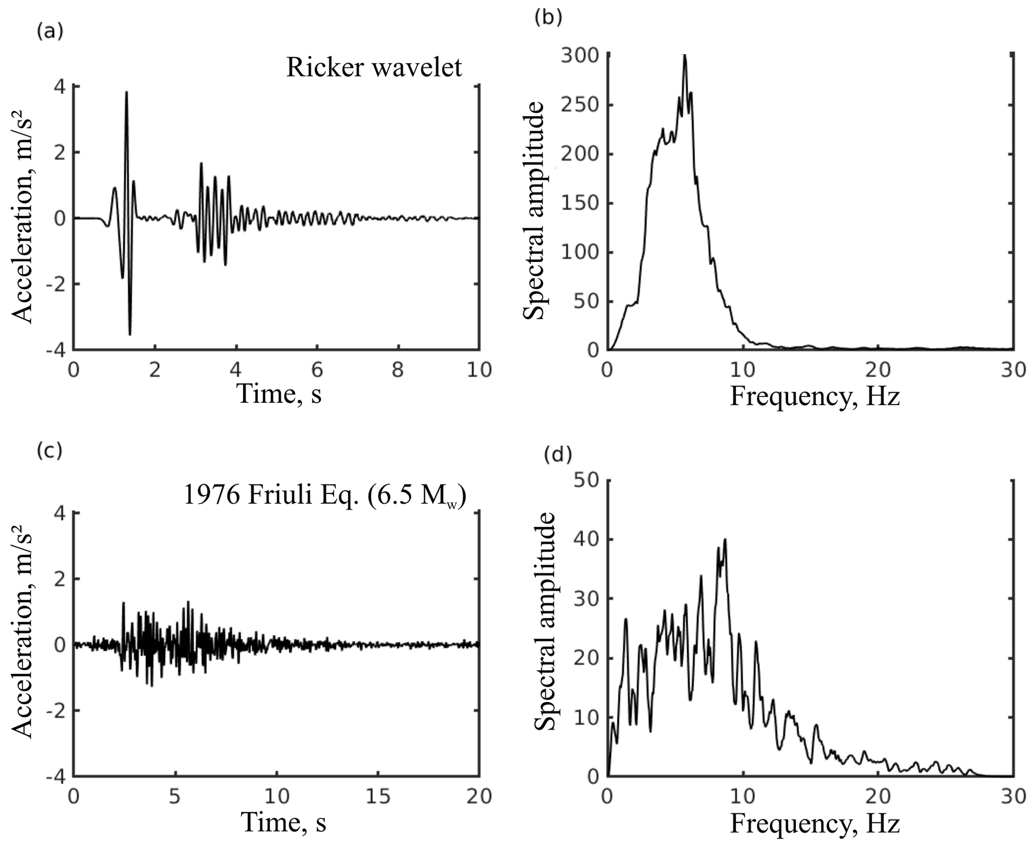
Figure 7Seismic signals in the time and frequency domain. (a, b) Ricker wavelet (as recorded at the model base monitoring point); (c, d) 1976 Friuli earthquake (Italy). Note the different timescales.
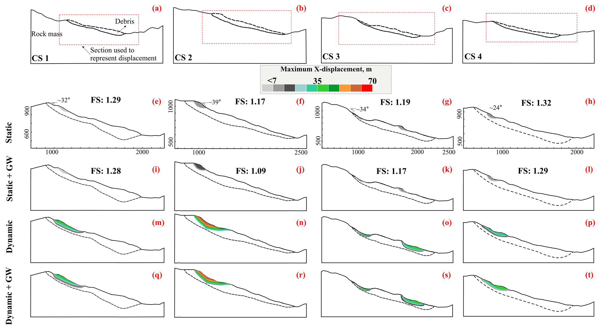
Figure 8Factor of safety (FS) and material displacement (x direction). Panels (a)–(d) refer to original slope sections with sub-sections (red rectangle) used to represent displacement. Panels (e)–(t) refer to displacement in static, static + GW, dynamic, and dynamic + GW conditions.
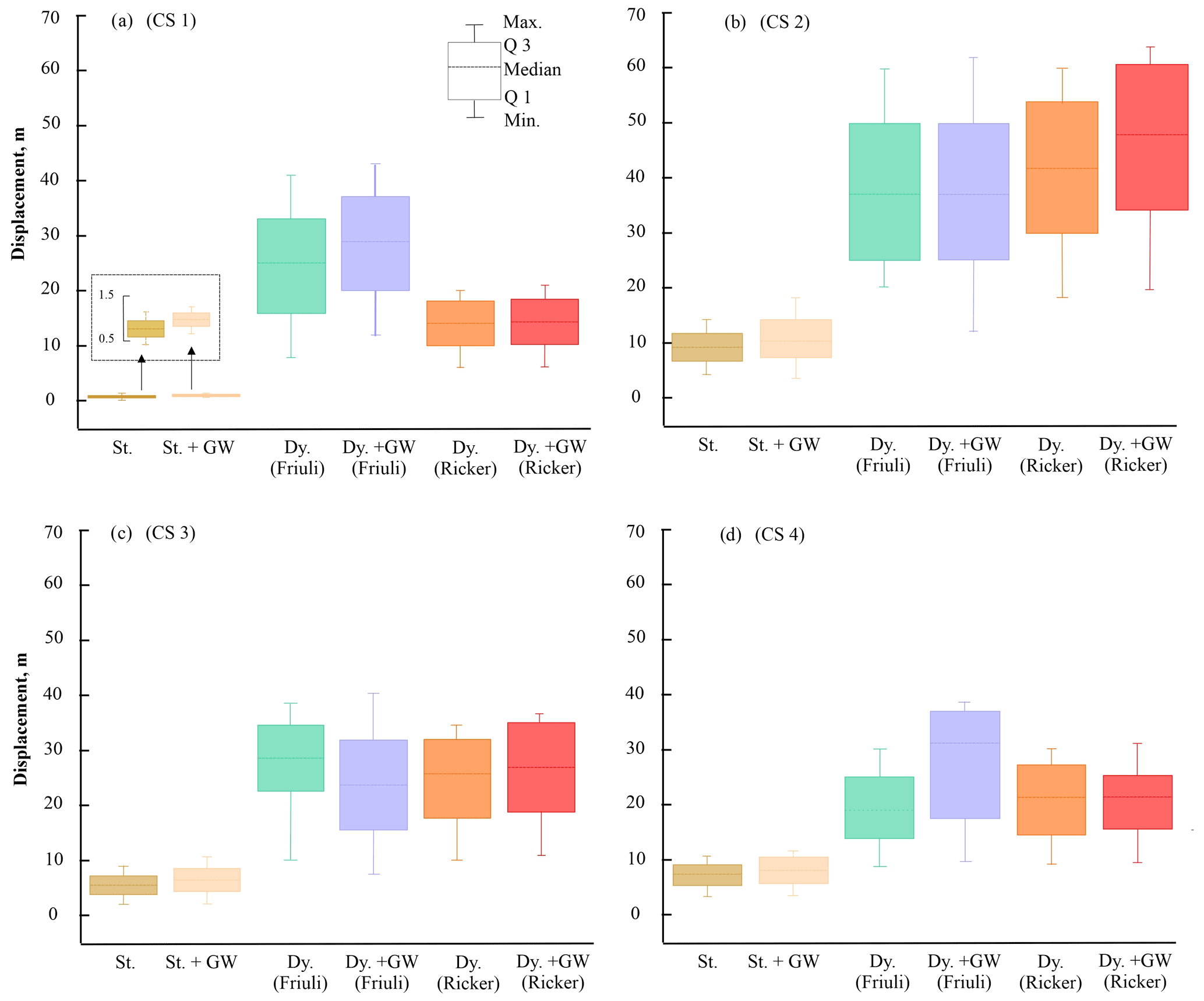
Figure 9Comparison of material displacement under different conditions. St. and Dy. refer to static and dynamic conditions, respectively. GW refers to groundwater.
As also shown in Fig. 9, the GW conditions enhanced the displacement in static as well as in dynamic conditions (Fig. 9). Static displacement showed the least scattering as evident from the median level and least difference in max and min values. Further, except for the CS-2 section, all three sections (CS-1, CS-3, CS-4) have relatively low dynamic displacement in dry and wet (GW) conditions due to the Ricker wavelet compared to the displacement caused by the Friuli signal (Fig. 9a–d). This difference may be attributed to the response of steep topography (of the CS-2 model) to the high-energy Ricker wavelet signal (Fig. 7b).
Thus, it can be understood that the Varlaam hillslope, situated in the region having frequent extreme rainfalls and earthquakes, attains more instability under saturated dynamic conditions.
4.1.2 Parametric analysis
The factor of safety (FS) of the slope increased in response to increase in the angle of internal friction of soil, joint friction, and elastic modulus (Fig. 10). Such increase in the FS (∼7 % in the CS-2) is attained by increasing the angle of internal friction of soil. This effect is attributed to the “shear strength reduction” (SSR) approach. The GW level increase resulted in a decreasing FS because the increased GW level increased the joint flow rate and thus enhanced the fluid pressure on the overlying medium, i.e., soil. This increased fluid pressure further decreased the normal stress and hence the shear stress of the overlying soil, as per Mohr's criteria (Mohr, 1914). Such decrease in the shear stress of soil resulted in the decreased FS.
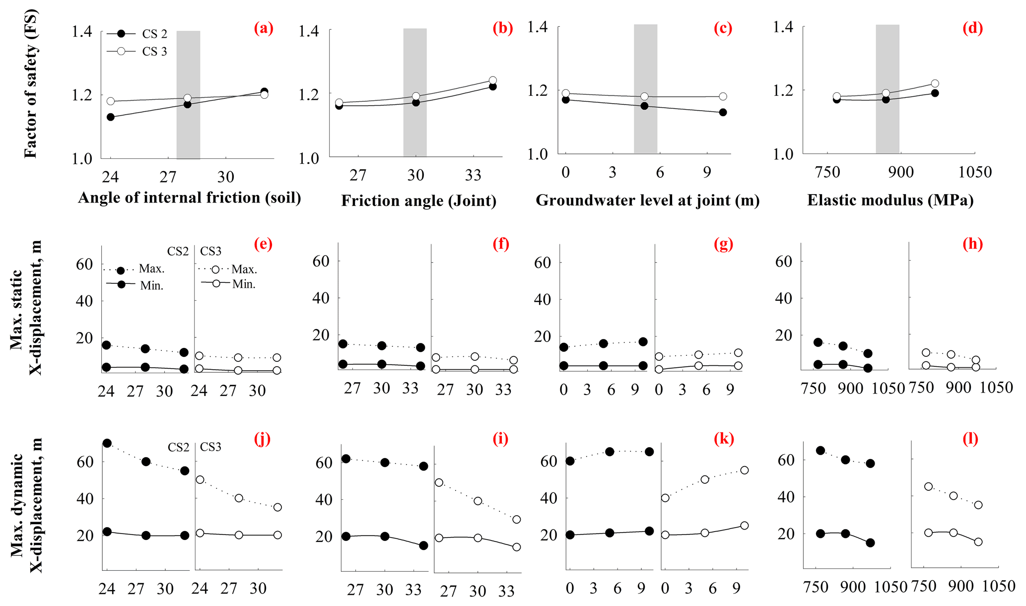
Figure 10Parametric analysis. (a–d) Variation in the FS. (e–h) Variation in the static displacement. (i–l) Variation in the dynamic displacement. Grey bar represents the values that are used in the slope stability analysis (Sect. 4.1). Notably, vertical axes in (e)–(l) are kept the same to show relative increase in displacement under static and dynamic conditions.
Owing to their spatially variable nature, static and dynamic displacements are represented in ranges of the maximum (max) and minimum (min) in Fig. 10. Static displacement decreased on increasing the angle of internal friction of soil, joint friction, and elastic modulus. Such decrease (∼40 % in CS-2 and ∼38 % in CS-3) occurred in response to the modulus increase. This decrease in the displacement refers to the fact that the increased modulus increases the normal and shear strength of the soil, and hence displacement will decrease on increasing the modulus (Hara et al., 1974). The GW level increase resulted in the increased static displacement (∼16 % in CS-2, ∼36 % in CS-3). Such increase in the static displacement is attributed to the decreased shear strength of soil due to the increased joint fluid pressure (Witherspoon et al., 1980). Similarly to the static displacement, dynamic displacement decreased on increasing the angle of internal friction of soil, joint friction, and elastic modulus and increased on increasing the GW level. Along with the modulus, the angle of internal friction of soil is also noted to decrease (∼16 % in CS-2, ∼21 % in CS-3) the dynamic displacement more. The increase in the GW level resulted in 8 % and 33 % increases in the CS-2 and CS-3 models, respectively, in dynamic displacement.
Notably, the present study utilized approximated values of the input parameters for the slope stability analysis (Table 1). Though the approximated values cannot replace the values measured in the geotechnical analysis, parametric analysis minimizes the uncertainty caused by the selection of specific values by exploring the possible output pattern.
Thus, by utilizing the central values (highlighted as grey in Fig. 10) in the slope stability analysis (Sect. 4.1.1), the present study attempted to minimize such uncertainty in the findings. Further, though the GW was also used in the UDEC models to infer the influence of saturation on slope stability, the potential response of the slope under excessive saturation (extreme rainfall) is further explored using the debris flow runout simulation (Sect. 4.2).
4.1.3 Peak ground acceleration (PGA)
Apart from the FS and displacement, ground motion (acceleration) amplification was also evaluated to understand the potential seismic deformation at the slope surface (Fig. 11). The input seismic signal for the following acceleration pattern is presented in Fig. 7a. For all four models (CS-1 to CS-4), the PGA values at the river floor (RF) ranges between 5.78–7.47 m s−1 (0.58–0.74 g), whereas at the rock mass surface above the landslide crown (CR) they vary from 6.37 to 10.19 m s−1 (0.65–1.03 g) (Fig. 11). At the model base (MB), maximum acceleration remains between 3.79–3.90 m s−1 (0.38–0.39 g).
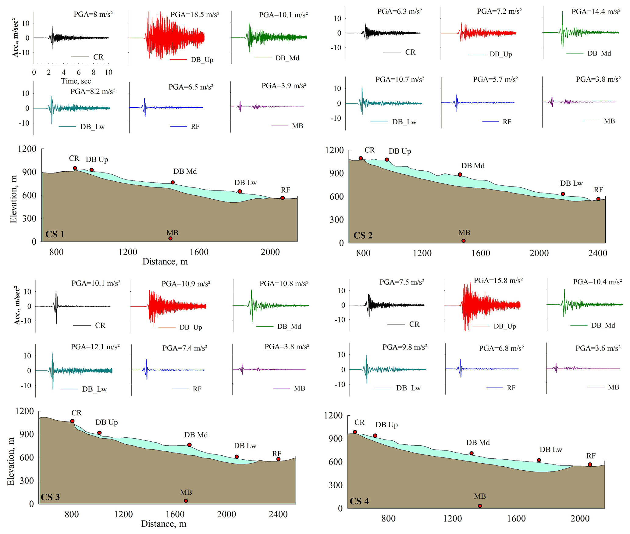
Thus, the PGA at the RF is amplified by ∼1.5–2.0 times the maximum acceleration at the model base, whereas at the rock mass surface above the landslide crown, it is amplified by ∼1.7–2.7 times the maximum acceleration at the model base. Such amplification of the PGA at the rock mass surface above the landslide crown can be attributed to the topographic irregularity and upward propagation of seismic waves where they meet preceding waves produced on the relatively horizontal surface of the slope (Jibson, 1987; Havenith et al., 2003; Bourdeau and Havenith, 2008; Luo et al., 2020).
The debris surface, however, attains higher PGA in all four models than the rock mass surface as noted at the following three monitoring stations: DB_Lw, DB_Md, and DB_Up (Fig. 11). At the lower part of the debris (DB_Lw), the PGA ranges from 8.3 to 12.13 m s−1 (0.84–1.23 g) and further grew at the middle part of the debris (DB_Md), attaining 10.17–14.40 m s−1 (1.03–1.46 g). The maximum PGA is attained by the upper part of the debris (DB_Up) with a range of 7.26–18.50 m s−2 (0.74–1.88 g). Such relatively high PGA at the debris surface can be linked to the impedance contrast between underlying rock mass and overlying soil and/or partial loss of the shear strength during seismicity (Novak and Han, 1990; Šafak, 2001).
Detailed evaluation at different monitoring points in each model is as follows: model base (MB) and river floor (RF) monitoring points have almost similar maximum acceleration values in all four models. At the lower part of the debris, i.e., DB_Lw, higher PGA is attained by the CS-3 model (∼12.1 m s−2) followed by the CS-2 model (∼10.8 m s−1) in comparison to DB_Low points of CS-1 and CS-4. Higher PGA is attributed to lower soil thickness below this monitoring point in the CS-3 and CS-2 models that could be the main reason for acceleration amplification as also stated by Murphy et al. (1971) and Beresnev and Wen (1996).
At the middle part of the debris, i.e., DB_Md, higher PGA is attained by the CS-2 model (∼14.4 m s−2). Notably, despite the higher soil thickness, this monitoring point obtained a higher PGA. It possibly occurred due to irregular topography of the CS-2 model that generally results in interference of direct and scattered waves and hence amplification of ground motions (Asimaki and Mohammadi, 2018).
At the upper part of the debris, i.e., DB_Up, higher PGA is attained by the CS-1 model (18.5 m s−2) followed by the CS-4 model (15.8 m/s−2). The effect of soil thickness below this monitoring point, as explained for the lower part of debris, could be the main reason for such amplification at this monitoring point in these models. The monitoring point at the rock mass surface above the landslide crown (CR) also has almost similar PGA values in all the models except the CS-3 model. Higher PGA (10.19 m s−2) at the CR monitoring point of the CS-3 model might be due to its position on a steeper surface, whereas CR points in other models are at a relatively flat surface.
4.1.4 Spectral ratio
The ground motion amplifications were also explored using the spectral ratios at two central slope sections: CS-2 and CS-3 (Fig. 12). In both models, the RF (river floor) point showed no significant amplification at any particular frequency, possibly due to the flat surface positioning. In the CS-2 model, the debris lower part (DB_Lw) point shows notable amplification at 2.0–2.5 Hz with minor amplification at 4.5–5.0 Hz, whereas in the CS-3 model, the DB_Lw point shows attenuation (or de-amplification) near ∼2 Hz and slight amplification at 4.5–6.0 Hz. The contrast of amplification and de-amplification at ∼2 Hz is attributed to the geometrical variation in topography because the DB_Lw point in CS-2 is situated at a relatively elevated surface, whereas in CS-3, it is at a relatively shallow surface. Minor geometrical variations at the slope toe have been also observed to result in de-amplification at low frequencies in other studies (Bouckovalas and Papadimitriou, 2005).
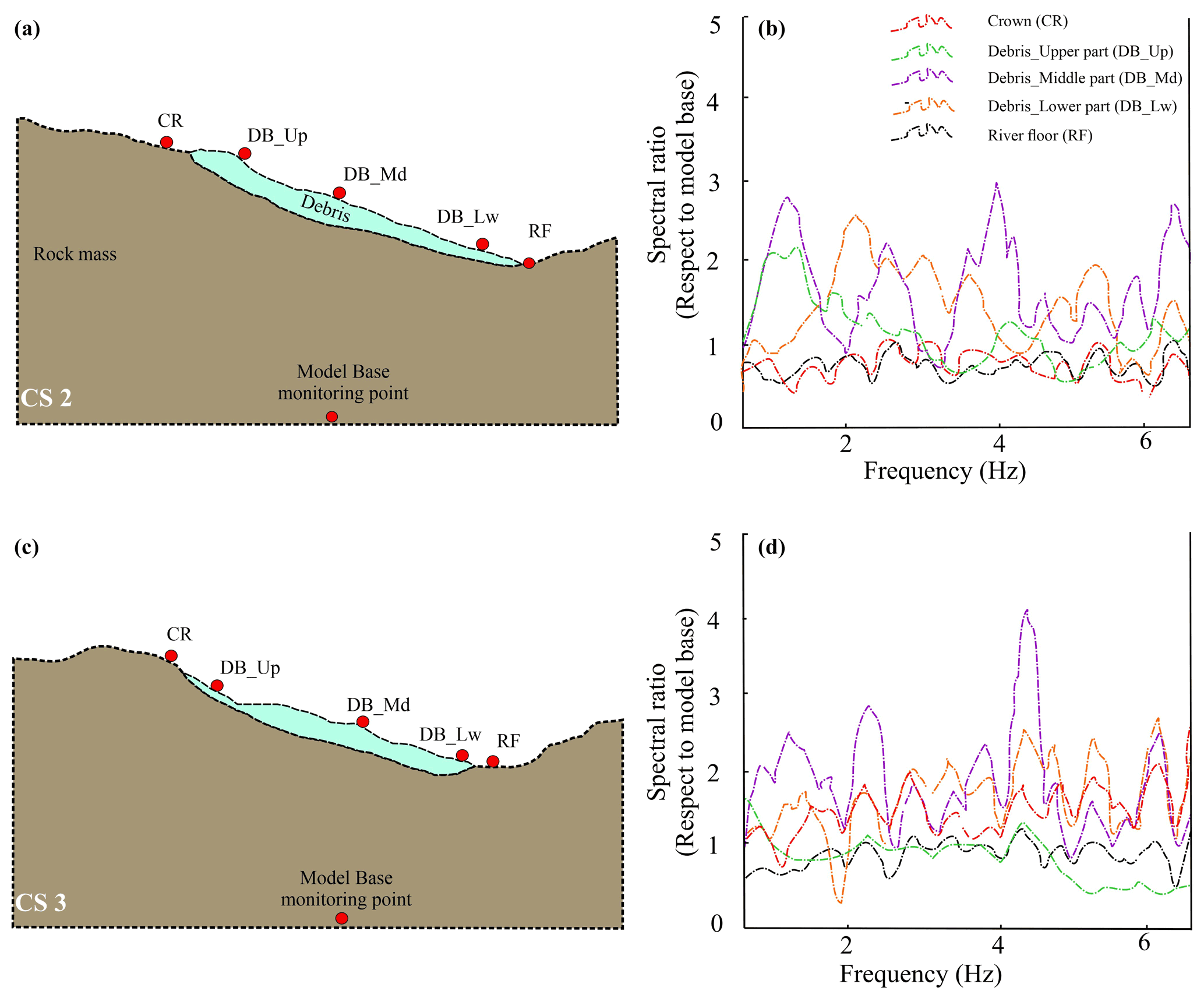
Figure 12Spectral ratio pattern. (a) CS-2 model with the position of monitoring points. (b) Spectral ratio pattern in CS-2. (c) The CS-3 model with the position of monitoring points. (d) Spectral ratio pattern in CS-3.
Notably, along with the DB_Lw point, the debris middle part (DB_Md) and debris upper part (DB_Up) points in both the models also have minor/major amplification at 4.5–6.0 Hz. This coexistence of amplification at a certain frequency range by different monitoring points at the debris surface may be attributed to impedance contrast between debris and underlying rock mass. Further, the DB_Md point in both the models showed amplification at ∼1.0 and 2.0–2.5 Hz. The amplification at a lower frequency, i.e., ∼1.0 Hz, may be attributed to the thick (40–60 m) layer of debris that possibly decreases the resonance frequency and results in amplification of ground motion as also reported by Beresnev and Wen (1996). The amplification at 2.0–2.5 Hz may be linked to the elevated topography at these points in both the models.
The DB_Up point in both the models has different responses. In the CS-2 model, it showed amplification at 1.0–1.5 Hz, whereas in the CS-3 model, the spectral ratio is relatively stagnant except minor amplification at 4.0 and 6.0 Hz. This contrast may be understood by the fact that in CS-2, this monitoring point is situated at a thicker and elevated surface, whereas in CS-3, it is situated at relatively shallow topography and on top of relatively thin landslide thickness. Finally, the crown (CR) point also has a different spectral ratio in both the models. It shows higher amplification in the CS-3 model than the CS-2 model, which may be linked to the positioning of these points. The CR in the CS-2 is situated at a relatively flat surface unlike in the CS-3 model where it is situated at a steep surface. Thus, the monitoring points showed amplification at multiple frequency ranges that are attributed to the complex topography of landslides, soil thickness variation, and impedance contrast.
4.2 Landslide runout pattern
In view of uncertainties in ascertaining the exact depth of loose material that will be eroded/entrained during the debris flow, the runout pattern was evaluated at four different release area depths: 5, 10, 15, and 20 m of the loose overburden (Fig. 13a and b). The identification of the release area was based on field and satellite imagery observations. Four factors – gullies (Fig. 2c), flow relics (Fig. 2d), signs of failure (Fig. 2e), and overburden thickness pattern (Fig. 5c) – were considered while selecting the release area. The thickness region of 60–80 m having flow relics and signs of failure was therefore selected as the potential release area (Fig. 13b). Debris flow characteristics (flow height and flow velocity) of the debris flow that will strike the river floor during such an event are also inferred along the river channel (Fig. 13c). The debris flow height and velocity at the hillslope and along the river channel are summarized in Table 3.

Figure 13Debris flow runout pattern. (a) Soil (or debris) thickness pattern in the landslide. (b) Different release area depths (5, 10, 15, and 20 m) used for the analysis. (c) River profile section A–B used to represent the resultant debris flow along the river. (d–f) Results at 5 m depth. (g–i) Results at 10 m depth. (j–l) Results at 15 m depth. (m–o) Results at 20 m depth.
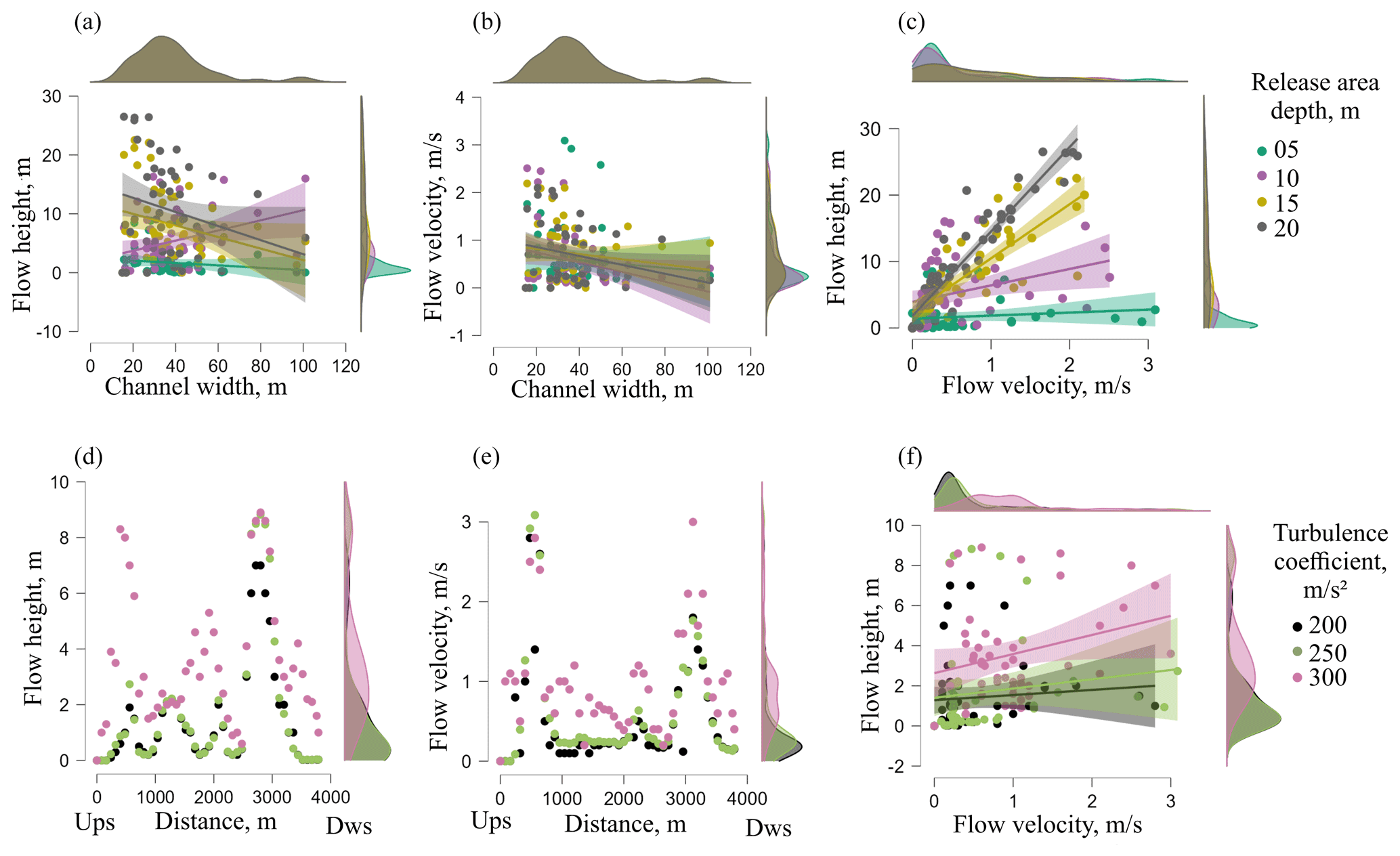
Figure 14Relationship of channel width and debris flow characteristics (a–c) and results of sensitivity analysis at constant “maximum” friction and variable turbulence (d–f). “Ups” and “Dws” refer to the upstream and downstream sides of the river channel, respectively.
Table 3Results of the runout simulation at different depths of the release area.

As can be seen from Fig. 13, increasing depth of the release area increases the flow characteristics at the hillslope. However, the flow characteristics vary once the flow strikes the river floor. Debris flow height increases towards downstream part of the river channel on increasing the depth of material (Fig. 13f, i, l, and o). This behavior can be linked to the gully/channel on the hillslope near the downstream part (Fig. 2c) that possibly accelerated the flow. Debris flow velocity, however, decreases on increasing the depth of material. Higher flow velocity at lower material depth (Fig. 13f) can be understood using the “turbulence (or Chézy resistance) ξ” factor used in Eq. (3). The Chézy resistance is famous as “turbulent” friction (Voellmy, 1955) since its mathematical formulations are similar to the well-known turbulent Chézy equation (Chow, 1959). According to the Chézy equation, lower material thickness results in higher flow velocity. Further, apart from such turbulence effects, river channel morphology also affects the flow characteristics. As can be seen in Fig. 14a–c, a smaller channel width (narrow sections) generally accommodates higher flow velocity and height, of course with some nonlinearity as seen at 10 m depth (Fig. 14a). Further, increasing the material depth increases the flow height more than flow velocity (Fig. 14c).
By keeping the maximum friction (μ=0.4) constant, a sensitivity analysis was also performed by using different turbulence coefficients (Fig. 14d–f). It revealed that flow height and velocity increase on increasing the turbulence coefficient (implying increasing liquid content). It is of note that the central value, i.e., 250 m s−2, showing a moderate response, is used in the main findings, as also mentioned in Table 2. Further, flow velocity is found to be more responsive at lower turbulence, whereas at higher turbulence, flow height dominates (Fig. 14f). Further, in order to understand the extent of runout along the river channel, runout results at the maximum release area depth were also laid over Google Earth imagery (Fig. 15a and b). A top view of the landslide with the runout is shown in inset c. The predicted runout is noted to extend across the river channel mainly at two locations, one near the left flank (Fig. 15d) and the other near the right flank (Fig. 15e). At both of these locations, the river channel attains sinuosity in a range of ∼1.30–1.32 (shown through channel length measurement). The river channel might owe this sinuosity to the paleo-landslide and/or fluvial deposit that extends the slope toe at these locations. Thus, the runout findings of the present study are noted to follow the same spatial extent as possibly followed by previous landslide events.
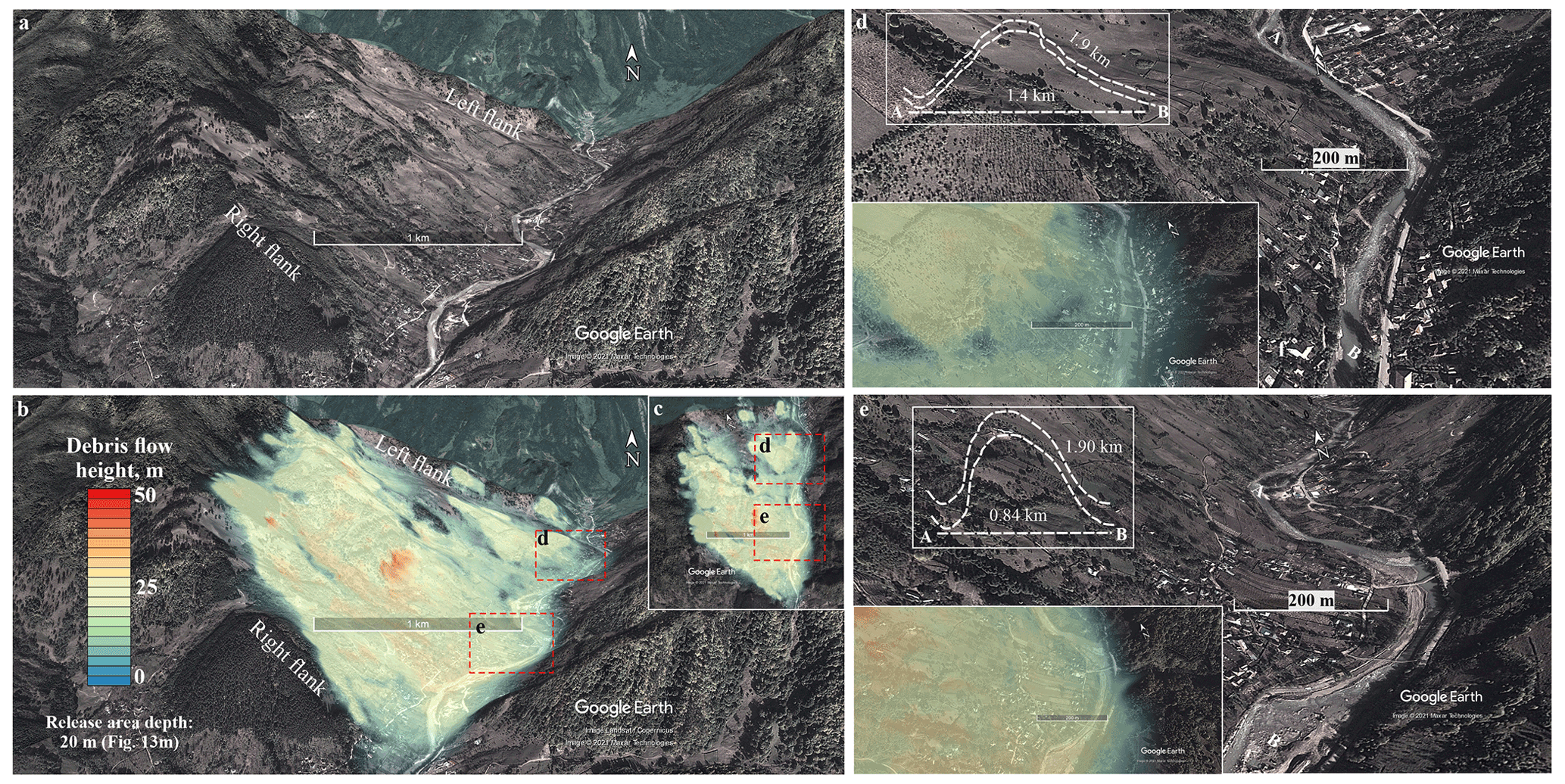
Figure 15Debris flow runout pattern at 20 m depth. (a) Upstream view of the landslide from the right flank. (b) Runout pattern at 20 m depth. (c) Top view of the landslide highlighting two regions where runout reached across the river. (d) Runout pattern near the left flank extending across the river channel. (e) Runout pattern near the right flank extending across the river channel.
The present state of the slope reveals an instability condition through the factor of safety in a range of 1.09–1.32 and potential displacement near the landslide crown (Figs. 8 and 9). Such a displacement near the landslide crown may be related to the development of shear failure in slopes (Matsui and San, 1992; Kumar et al., 2018, 2021). The possibility of shear failure becomes more viable in the case of degradation of the shear strength of slope material and/or rupture planes. Notably, both the main landslide-triggering factors – rainfall and earthquakes – have been found to degrade the shear strength of slope material through percolation and shaking-induced particle movements, respectively (Cai and Ugai, 2004; Chang and Taboada, 2009). The GW, implying the rainfall-induced percolation effect, decreases the factor of safety and increases the material displacement. This effect is attributed to the joint hydraulic pressure against the overlying loose material that decreases the normal stress and hence the shear strength of overlying loose material (Mohr, 1914; Witherspoon et al., 1980). Similarly to the GW effect in static conditions, the combined response of the dynamic force and the GW resulted in an increase in the displacement (Fig. 8). This can be attributed to the fact that seismic shaking increases the hydraulic pressure in the joints that causes enhanced material displacement in the overlying loose material (Wang et al., 2010).
Further, the ground motion amplification also revealed the slope instability (or potential deformation). The maximum value of peak ground acceleration (PGA) is attained by the upper part of the debris surface (near the landslide crown) (Fig. 11). It is linked to the impedance contrast between underlying rock mass and overlying soil and/or partial loss of the shear strength during seismicity (Novak and Han, 1990; Šafak, 2001). Further, the spectral ratio also showed signal amplification, at multiple frequency ranges, at the debris surface (Fig. 12). Such an amplification at multiple frequency ranges is attributed to the complex topography of landslides, soil thickness variation, and impedance contrast (Sect. 4.1.4). Such high amplification at the slope surface has also been considered a main cause of slope failure in many other studies (Lenti and Martino, 2012; Del Gaudio et al., 2019).
As also stated in Sect. 3.3, hillslopes affected by the seismic shaking have also been prone to rainfall-induced failures, particularly in the form of debris flows. Further, the earthquake-induced shear strength degradation of slope material may also result in enhanced entrainment during a debris flow event (Liu et al., 2020). These debris flows might be initiated by either increased pore pressure (or GW-induced hydraulic pressure) or runoff involving entrainment (Godt and Coe, 2007). Though the GW effect is seen in the slope instability (Figs. 8 and 9), the potential response of the slope under excessive rainfall is explored through debris flow runout analysis (Figs. 13–15).
The debris flow runout predictions revealed a nonlinear increase in the debris flow height and velocity along the river channel on increasing the depth of the release area (Fig. 13). This nonlinearity is attributed to the variation in the river channel width (Fig. 14) and influx of debris flow material from the slope. Though the present study noted the influence of channel morphology on the debris flow characteristics, other studies have observed the changes in channel morphology caused by debris flows (Remaître et al., 2005; Simoni et al., 2020).
Thus, there seems to be a positive feedback process between channel morphology and debris flow that is further strengthened by the finding of the debris flow extent across the river channel (Fig. 15d and e). At both of these locations, the slope toe extends towards the ESE direction, resulting in higher channel sinuosity. These extended slope toes probably represent paleo-landslide and/or fluvial deposits. Signs of flow relics at the slope surface and failure at the slope toe at these locations (Fig. 2d and e) further support the possibility of paleo-landslide deposits. Thus, the predicted extent of potential debris flow is found to follow the trails possibly created by previous landslide flow and/or slide events. Aforementioned findings – temporally increasing rainfall, soil moisture, and surface runoff (Sect. 2.2) – and frequent debris flows/flash floods in this region (Micu et al., 2013; Grecu et al., 2017; Micu, 2019) pose an increasing risk of debris flow in the study area.
Finally, there are still some uncertainties in such predictive approaches that are as follows: (1) the inclusion of the subsurface discontinuity network, spatially varying groundwater surface, and material heterogeneity in the 3D model and (2) the inclusion of variable depth and phases in the runout modeling. Despite these possible uncertainties, which will be overcome in future work, such studies are required to minimize the risk and avert possible disasters.
By utilizing field-based data and numerical simulations of a massive (∼9.1 Mm2) Varlaam landslide in the SE Carpathians (Romania), the present study explored the potential response of this landslide in a seismic and rainfall regime.
The slope revealed the factor of safety in a range of 1.09–1.32 along with a static displacement of 0.4–4 m that increases up to 8–60 m under seismic load. The groundwater, implying the saturation, further decreased the slope stability owing to enhanced joint hydraulic pressure. Ground motion amplification, during seismic shaking, further revealed the potential instability of the slope with a peak ground acceleration (PGA) on the slope surface in a range of 0.65–1.88 g. Such amplification pertains to the complex topography of landslides, soil thickness variation, and impedance contrast.
Further, though the GW effect is seen in the slope instability, the potential response of the slope under excessive rainfall is also evaluated through debris flow runout analysis. The predicted debris flow revealed a nonlinear increase in the debris flow height (9.0–26.0 m) and velocity (2.1–3.0 m s−1) along the river channel. This variation along the river channel is attributed to the river channel morphology and influx of debris flow material from the slope. Owing to the predictive nature of the present study, the concept may be applied to other terrains subjected to frequent landslides mostly triggered by extreme rainfall and earthquakes.
Slope stability analysis and debris flow runout simulations are performed using UDEC v.6 and RAMMS v.1.7.0 (both commercial software), respectively. Figures are prepared using CorelDRAW 2021 (commercial software) and JASP v.0.15 (open source).
Monthly (rainfall, soil moisture, and surface runoff) and daily rainfall datasets are openly accessible at https://giovanni.gsfc.nasa.gov/giovanni/ (NASA, 2021). The earthquake distribution dataset of the study area is available on request at http://www.infp.ro/ (National Research and Development Institute for Earth Physics, 2021).
The supplement related to this article is available online at: https://doi.org/10.5194/nhess-21-3767-2021-supplement.
VK and HBH conceived the idea. All authors participated in the field data collection and data interpretation. VK, LC, and ASM performed the numerical simulations. MM led the geomorphic interpretation. All authors contributed to the writing of the final draft.
The contact author has declared that neither they nor their co-authors have any competing interests.
Publisher's note: Copernicus Publications remains neutral with regard to jurisdictional claims in published maps and institutional affiliations.
This article is part of the special issue “Earthquake-induced hazards: ground motion amplification and ground failures”. It is a result of the EGU General Assembly 2021, 19–30 April 2021.
The authors acknowledge Philippe Cerfontaine, Martin Depret, Nirmit Dhabaria, and George Catalin Simion for data acquisition (DGPS and seismological measurements). Vipin Kumar is also thankful to Imlirenla Jamir for the constructive discussion related to hydrological parameters.
Authors are thankful for the financial grant by the F. R. S.– FNRS Belgium in the frame of the Belgian–Swiss collaboration project “4D seismic response and slope failure”.
This paper was edited by Giovanni Forte and reviewed by Tapas Martha and one anonymous referee.
Apostol, L.: The Mediterranean cyclones–the role in ensuring water resources and their potential of Apostol, L., 2008. The Mediterranean cyclones – the role in ensuring water resources and their potential of climatic risk, in the east of Romania, Present Environ. Sustain. Dev., 2, 143–163, 2008.
Asimaki, D. and Mohammadi, K.: On the complexity of seismic waves trapped in irregular topographies, Soil Dynam. Earthq. Eng., 114, 424–437, 2018.
Barton, N. and Choubey, V.: The shear strength of rock joints in theory and practice, Rock Mech., 10, 1–54, 1977.
Barton, N. R.: A model study of rock-joint deformation, Int. J. Rock Mech. Min., 9, 579–602, 1972.
Bednarczyk, Z.: Identification of flysch landslide triggers using conventional and `nearly real-time' monitoring methods – An example from the Carpathian Mountains, Poland, Eng. Geol., 244, 41–56, 2018.
Beguería, S., Van Asch, Th. W. J., Malet, J.-P., and Gröndahl, S.: A GIS-based numerical model for simulating the kinematics of mud and debris flows over complex terrain, Nat. Hazards Earth Syst. Sci., 9, 1897–1909, https://doi.org/10.5194/nhess-9-1897-2009, 2009.
Beresnev, I. A. and Wen, K. L.: Nonlinear soil response – A reality?, Bull. Seismol. Soc. Am., 86, 1964–1978, 1996.
Bhasin, R. and Kaynia, A. M.: Static and dynamic simulation of a 700-m high rock slope in western Norway, Eng. Geol., 71, 213–226, 2004.
Biggs, J. M.: Introduction to structural dynamics, McGraw-Hill College, USA, 1964.
Bokelmann, G. and Rodler, F. A.: Nature of the Vrancea seismic zone (Eastern Carpathians) – New constraints from dispersion of first-arriving P-waves, Earth Planet. Sc. Lett., 390, 59–68, 2014.
Bontemps, N., Lacroix, P., Larose, E., Jara, J., and Taipe, E.: Rain and small earthquakes maintain a slow-moving landslide in a persistent critical state, Nat. Commun., 11, 1–10, 2020.
Bouckovalas, G. D. and Papadimitriou, A. G.: Numerical evaluation of slope topography effects on seismic ground motion, Soil Dynam. Earthq. Eng., 25, 547–558, 2005.
Bourdeau, C. and Havenith, H. B.: Site effects modelling applied to the slope affected by the Suusamyr earthquake (Kyrgyzstan, 1992), Eng. Geol., 97, 126–145, 2008.
Cai, F. and Ugai, K.: Numerical analysis of rainfall effects on slope stability, Int. J. Geomech., 4, 69–78, 2004.
Cauchie, L., Mreyen, A. S., Micu, M., Cerfontaine, P., and Havenith, H. B.: Landslide characterization by seismic ambient noise analysis: application to Carpathian Mountains, in: AGU Fall Meeting, 9–13 December 2019, San Francisco, https://doi.org/10.13140/RG.2.2.18971.69924, 2019.
Chang, K. J. and Taboada, A.: Discrete element simulation of the Jiufengershan rock-and-soil avalanche triggered by the 1999 Chi-Chi earthquake, Taiwan, J. Geophys. Res.-Earth, 114, F03003, https://doi.org/10.1029/2008JF001075, 2009.
Chow, V. T.: Open-channel hydraulics, in: McGraw-Hill civil engineering series, McGraw-Hill, Tokyo, 1959.
Christen, M., Kowalski, J., and Bartelt, P.: RAMMS: Numerical simulation of dense snow avalanches in three-dimensional terrain, Cold Reg. Sci. Technol., 63, 1–14, 2010.
Constantin, S., Bojar, A. V., Lauritzen, S. E., and Lundberg, J.: Holocene and Late Pleistocene climate in the sub-Mediterranean continental environment: A speleothem record from Poleva Cave (Southern Carpathians, Romania), Palaeogeogr. Palaeocl., 243, 322–338, 2007.
Coulomb, C. A.: An attempt to apply the rules of maxima and minima to several problems of stability related to architecture, Mémoires de l'Académie Royale des Sciences, 7, 343–382, 1776.
Croitoru, A. E., Piticar, A., and Burada, D. C.: Changes in precipitation extremes in Romania, Quatern. Int., 415, 325–335, 2016.
Del Gaudio, V., Zhao, B., Luo, Y., Wang, Y., and Wasowski, J.: Seismic response of steep slopes inferred from ambient noise and accelerometer recordings: the case of Dadu River valley, China, Eng. Geol., 259, 105197, https://doi.org/10.1016/j.enggeo.2019.105197, 2019.
Ding, M., Huang, T., Zheng, H., and Yang, G.: Respective influence of vertical mountain differentiation on debris flow occurrence in the Upper Min River, China, Scient. Rep., 10, 1–13, 2020.
Durand, V., Mangeney, A., Haas, F., Jia, X., Bonilla, F., Peltier, A., Hibert, C., Ferrazzini, V., Kowalski, P., Lauret, F., and Brunet, C.: On the link between external forcings and slope instabilities in the Piton de la Fournaise Summit Crater, Reunion Island, J. Geophys. Res.-Earth, 123, 2422–2442, 2018.
Fell, R. and Hartford, D.: Landslide risk management, Landslide Risk Assess., 51–110, https://doi.org/10.1201/9780203749524-4, 1997.
Fenton, G. A. and Griffiths, D. V.: Risk assessment in geotechnical engineering, in: Vol. 461, John Wiley & Sons, New York, 2008.
Froude, M. J. and Petley, D. N.: Global fatal landslide occurrence from 2004 to 2016, Nat. Hazards Earth Syst. Sci., 18, 2161–2181, https://doi.org/10.5194/nhess-18-2161-2018, 2018.
Gholamy, A. and Kreinovich, V.: Why Ricker wavelets are successful in processing seismic data: Towards a theoretical explanation, in: 2014 IEEE Symposium on Computational Intelligence for Engineering Solutions (CIES), 9–12 December 2014, Florida, 11–16, 2014.
Godt, J. W. and Coe, J. A.: Alpine debris flows triggered by a 28 July 1999 thunderstorm in the central Front Range, Colorado, Geomorphology, 84, 80–97, 2007.
Grecu, F., Zaharia, L., Ioana-Toroimac, G., and Armaş, I.: Floods and flash-floods related to river channel dynamics, in: Landform dynamics and evolution in Romania, Springer, Cham, 821–844, 2017.
Griffiths, D. V. and Lane, P. A.: Slope stability analysis by finite elements, Geotechnique, 49, 387–403, 1999.
Gupta, V., Jamir, I., Kumar, V., and Devi, M.: Geomechanical characterisation of slopes for assessing rockfall hazards in the Upper Yamuna Valley, Northwest Higher Himalaya, India, Himalaya. Geol., 38, 156–170, 2017.
Haque, U., Da Silva, P. F., Devoli, G., Pilz, J., Zhao, B., Khaloua, A., Wilopo, W., Andersen, P., Lu, P., Lee, J., and Yamamoto, T.: The human cost of global warming: Deadly landslides and their triggers (1995–2014), Sci. Total Environ., 682, 673–684, 2019.
Hara, A., Ohta, T., Niwa, M., Tanaka, S., and Banno, T.: Shear modulus and shear strength of cohesive soils, Soil. Foundat., 14, 1–12, 1974.
Havenith, H.-B., Strom, A., Calvetti, F., and Jongmans, D.: Seismic triggering of landslides. Part B: Simulation of dynamic failure processes, Nat. Hazards Earth Syst. Sci., 3, 663–682, https://doi.org/10.5194/nhess-3-663-2003, 2003.
Havenith, H. B., Torgoev, A., Braun, A., Schlögel, R., and Micu, M.: A new classification of earthquake-induced landslide event sizes based on seismotectonic, topographic, climatic and geologic factors, Geoenviron. Disast., 3, 1–24, 2016.
Helmstetter, A. and Garambois, S.: Seismic monitoring of Séchilienne rockslide (French Alps): Analysis of seismic signals and their correlation with rainfalls, J. Geophys. Res.-Earth, 115, F03016, https://doi.org/10.1029/2009JF001532, 2010.
Hoek, E. and Brown, E. T.: Practical estimates of rock mass strength, Int. J. Rock Mech. Min. Sci., 34, 1165–1186, 1997.
Hoek, E. and Diederichs, M. S.: Empirical estimation of rock mass modulus, Int. J. Rock Mech. Min. Sci., 43, 203–215, 2006.
Hoek, E., Carranza-Torres, C., and Corkum, B.: Hoek-Brown failure criterion – 2002 edition, Proc. NARMS-Tac, 1, 267–273, 2002.
Huffman, G.J., Stocker, E. F., Bolvin, D. T., Nelkin, E. J., and Jackson T.: GPM IMERG Final Precipitation L3 1 day 0.1 degree × 0.1 degree V06, edited by: Savtchenko, A., Goddard Earth Sciences Data and Information Services Center (GES DISC), Greenbelt, MD, https://doi.org/10.5067/GPM/IMERGDF/DAY/06, 2019.
Hungr, O.: A review of landslide hazard and risk assessment methodology. Landslides and engineered slopes, in: Experience, theory and practice, edited by: Aversa, S., Cascini, L., Picarelli, L., and Scavia, C., CRC Press, Boca Raton, Florida, 3–27, 2018.
Hungr, O., Morgan, G. C., and Kellerhals, R.: Quantitative analysis of debris torrent hazards for design of remedial measures, Can. Geotech. J., 21, 663–677, 1984.
Hürlimann, M., Rickenmann, D., Medina, V., and Bateman, A.: Evaluation of approaches to calculate debris-flow parameters for hazard assessment, Eng. Geol., 102, 152–163, 2008.
Hutter, K., Svendsen, B., and Rickenmann, D.: Debris flow modeling: A review, Contin. Mech. Thermodynam., 8, 1–35, 1994.
Ibs-von Seht, M. and Wohlenberg, J.: Microtremor measurements used to map thickness of soft sediments, Bull. Seismol. Soc. Am., 89, 250–259, 1999.
Ilinca, V.: Characteristics of debris flows from the lower part of the Lotru River basin (South Carpathians, Romania), Landslides, 11, 505–512, 2014.
Jakob, M., Hungr, O., and Jakob, D. M.: Debris-flow hazards and related phenomena, in: Vol. 739, Springer, Berlin, 2005.
Jamir, I., Gupta, V., Kumar, V., and Thong, G. T.: Evaluation of potential surface instability using finite element method in Kharsali Village, Yamuna Valley, Northwest Himalaya, J. Mount. Sci., 14, 1666–1676, 2017.
Jibson, R.: Summary of research on the effects of topographic amplification of earthquake shaking on slope stability, US Geological Survey, Reston, Virginia, 87–269, 1987.
Jing, L.: A review of techniques, advances and outstanding issues in numerical modelling for rock mechanics and rock engineering, Int. J. Rock Mech. Min. Sci., 40, 283–353, 2003.
Joyner, W. B. and Chen, A. T.: Calculation of nonlinear ground response in earthquakes, Bull. Seismol. Soc. Am., 65, 1315–1336, 1975.
Kahraman, S.: Evaluation of simple methods for assessing the uniaxial compressive strength of rock, Int. J. Rock Mech. Min. Sci., 38, 981–994, 2001.
Klimeš, J., Rosario, A. M., Vargas, R., Raška, P., Vicuña, L., and Jurt, C.: Community participation in landslide risk reduction: a case history from Central Andes, Peru, Landslides, 16, 1763–1777, 2019.
Kuhlemeyer, R. L. and Lysmer, J.: Finite element method accuracy for wave propagation problems, J. Soil Mech. Foundat. Div., 99, 421–427, 1973.
Kumar, V., Gupta, V., and Jamir, I.: Hazard evaluation of progressive Pawari landslide zone, Satluj valley, Himachal Pradesh, India, Nat. Hazards, 93, 1029–1047, 2018.
Kumar, V., Jamir, I., Gupta, V., and Bhasin, R. K.: Inferring potential landslide damming using slope stability, geomorphic constraints, and run-out analysis: a case study from the NW Himalaya, Earth Surf. Dynam., 9, 351–377, https://doi.org/10.5194/esurf-9-351-2021, 2021.
Lenti, L. and Martino, S.: The interaction of seismic waves with step-like slopes and its influence on landslide movements, Eng. Geol., 126, 19–36, 2012.
Liang, W. L.: Dynamics of pore water pressure at the soil–bedrock interface recorded during a rainfall-induced shallow landslide in a steep natural forested headwater catchment, Taiwan, J. Hydrol., 587, 125003, https://doi.org/10.1016/j.jhydrol.2020.125003, 2020.
Lin, C. W., Liu, S. H., Lee, S. Y., and Liu, C. C.: Impacts of the Chi-Chi earthquake on subsequent rainfall-induced landslides in central Taiwan, Eng. Geol., 86, 87–101, 2006.
Liu, Z., Su, L., Zhang, C., Iqbal, J., Hu, B., and Dong, Z.: Investigation of the dynamic process of the Xinmo landslide using the discrete element method, Comput. Geotech., 123, 103561, https://doi.org/10.1016/j.compgeo.2020.103561, 2020.
Luo, Y., Fan, X., Huang, R., Wang, Y., Yunus, A. P., and Havenith, H. B.: Topographic and near-surface stratigraphic amplification of the seismic response of a mountain slope revealed by field monitoring and numerical simulations, Eng. Geol., 271, 105607, https://doi.org/10.1016/j.enggeo.2020.105607, 2020.
Magyari, E. K., Demény, A., Buczkó, K., Kern, Z., Vennemann, T., Fórizs, I., Vincze, I., Braun, M., Kovács, J. I., Udvardi, B., and Veres, D.: A 13,600-year diatom oxygen isotope record from the South Carpathians (Romania): Reflection of winter conditions and possible links with North Atlantic circulation changes, Quatern. Int., 293, 136–149, 2013.
Margottini, C., Canuti, P., and Sassa, K.: Landslide science and practice, in: Vol. 1, Springer, Berlin, 2013.
Maţenco, L.: Tectonics and exhumation of Romanian Carpathians: inferences from kinematic and thermochronological studies, in: Landform dynamics and evolution in Romania, Springer, Cham, 15–56, 2017.
Matsui, T. and San, K. C.: Finite element slope stability analysis by shear strength reduction technique, Soil. Foundat., 32, 59–70, 1992.
McCowan, D. W. and Lacoss, R. T.: Transfer functions for the seismic research observatory seismograph system, Bull. Seismol. Soc. Am., 68, 501–512, 1978.
McDowell, P. W.: The determination of the dynamic elastic moduli of rock masses by geophysical methods, Engineering Geology Special Publications 6, Geological Society, London, 267–274, 1990.
McNally A.: FLDAS Noah Land Surface Model L4 Global Monthly 0.1×0.1 degree (MERRA-2 and CHIRPS), Goddard Earth Sciences Data and Information Services Center (GES DISC), Greenbelt, MD, USA, https://doi.org/10.5067/5NHC22T9375G, 2018.
Micu, M.: Landslide hazard assessment in Vrancea seismic region (Curvature Carpathians of Romania): achievements and perspectives, in: 1st EAGE Workshop on Assessment of Landslide and Debris Flows Hazards in the Carpathians, 17–20 June 2019, Lviv, Ukraine, 1–5, 2019.
Micu, M., Bălteanu, D., Micu, D., Zarea, R., and Raluca, R.: Landslides in the Romanian Curvature Carpathians in 2010, in: Geomorphological impacts of extreme weather, Springer, Dordrecht, 251–264, 2013.
Micu, M., Jurchescu, M., Şandric, I., Mărgărint, C., Zenaida, C., Dana, M., Ciurean, R., Ilinca, V., and Vasile, M.: Mass Movements, in: Landform dynamics and evolution in Romania, edited by: Radoane, M. and Vespremeanu-Stroe, A., Springer, Switzerland, 765–820, 2016.
Mihailovici, M., Gabor, O., Rândaşu, S., and Asman, I.: Floods in Romania, Hidrotehnica, 51, 23–35, 2006.
Mohr, O.: Abhandlungen aus dem Gebiete der Technischen Mechanik, 2nd Edn., Ernst, Berlin, 1914.
Mreyen, A. S., Cauchie, L., Micu, M., Onaca, A., and Havenith, H. B.: Multiple geophysical investigations to characterize massive slope failure deposits: application to the Balta rockslide, Carpathians, Geophys. J. Int., 225, 1032–1047, 2021.
Murgeanu, G., Dumitrescu, I., Sandulescu, M., Bandrabur, T., and Sandulesu, J.: Harta geologică a RS România, L-35-XXI, scara 1:200.000, Foaia Covasna, Institutul Geologic al României, Bucharest, Romania, 1965.
Murphy, J. R., Davis, A. H., and Weaver, N. L.: Amplification of seismic body waves by low-velocity surface layers, Bull. Seismol. Soc. Am., 61, 109–145, 1971.
Nakamura, Y.: Basic structure of QTS (HVSR) and examples of applications, in: Increasing seismic Safety by combining engineering technologies and seismological data, Springer, Dordrecht, 33–51, 2009.
NASA: Giovanni v 4.36, available at: https://giovanni.gsfc.nasa.gov/giovanni/, last access: 2 January 2021.
National Research and Development Institute for Earth Physics: Seismicitate recentă, available at: http://www.infp.ro/, last access: 11 March 2021.
Novak, M. and Han, Y. C.: Impedances of soil layer with boundary zone, J. Geotech. Eng., 116, 1008–1014, 1990.
Obreht, I., Zeeden, C., Hambach, U., Veres, D., Marković, S. B., Bösken, J., Svirčev, Z., Bačević, N., Gavrilov, M. B., and Lehmkuhl, F.: Tracing the influence of Mediterranean climate on Southeastern Europe during the past 350,000 years, Scient. Rep., 6, 1–10, 2016.
O'Brien, J. S., Julien, P. Y., and Fullerton, W. T.: Two-dimensional water flood and mudflow simulation, J. Hydraul. Eng., 119, 244–261, 1993.
Peranić, J., Moscariello, M., Cuomo, S., and Arbanas, Ž.: Hydro-mechanical properties of unsaturated residual soil from a flysch rock mass, Eng. Geol., 269, 105546, https://doi.org/10.1016/j.enggeo.2020.105546, 2020.
Petrescu, L., Stuart, G., Tataru, D., and Grecu, B.: Crustal structure of the Carpathian Orogen in Romania from receiver functions and ambient noise tomography: how craton collision, subduction and detachment affect the crust, Geophys. J. Int., 218, 163–178, 2019.
Pollock, W. and Wartman, J.: Human vulnerability to landslides, Geohealth, 4, e2020GH000287, https://doi.org/10.1029/2020GH000287, 2020.
Pospíšil, L., Hefty, J., and Hipmanová, L.: Risk and geodynamically active areas of the Carpathian lithosphere on the base of geodetical and geophysical data, Acta Geodaet. Geophys. Hungar., 47, 287–309, 2012.
Radulian, M., Bonjer, K. P., Popa, M., and Popescu, E.: Seismicity patterns in SE Carpathians at crustal and subcrustal domains: tectonic and geodynamic implications, in: Proceedings of the International Symposium on Strong Vrancea Earthquakes and Risk Mitigation, Bucharest, Romania, 4–6, 2007.
Remaître, A., Malet, J. P., and Maquaire, O.: Morphology and sedimentology of a complex debris flow in a clay-shale basin, Earth Surf. Proc. Land., 30, 339–348, 2005.
Rickenmann, D. and Scheidl, C.: Debris-flow runout and deposition on the fan, in: Dating torrential processes on fans and cones, Springer, Dordrecht, 75–93, 2013.
Ricker, N.: Further developments in the wavelet theory of seismogram structure, Bull. Seismol. Soc. Am., 33, 197–228, 1943.
Şafak, E.:Local site effects and dynamic soil behavior, Soil Dynam. Earthq. Eng., 21, 453–458, 2001.
Salm, B.: Flow, flow transition and runout distances of flowing avalanches, Ann. Glaciol., 18, 221–226, 1993.
Sassa, K.: ISDR-ICL Sendai Partnerships 2015–2025 for global promotion of understanding and reducing landslide disaster risk, Landslides, 12, 631–640, 2015.
Shieh, C. L., Chen, Y. S., Tsai, Y. J., and Wu, J. H.: Variability in rainfall threshold for debris flow after the Chi-Chi earthquake in central Taiwan, China, Int. J. Sediment Res., 24, 177–188, 2009.
Simoni, A., Bernard, M., Berti, M., Boreggio, M., Lanzoni, S., Stancanelli, L. M., and Gregoretti, C.: Runoff-generated debris flows: Observation of initiation conditions and erosion–deposition dynamics along the channel at Cancia (eastern Italian Alps), Earth Surf. Proc. Land., 45, 3556–3571, 2020.
Tang, C., Zhu, J., Qi, X., and Ding, J.: Landslides induced by the Wenchuan earthquake and the subsequent strong rainfall event: A case study in the Beichuan area of China, Eng. Geol., 122, 22–33, 2011.
Tischler, M., Matenco, L., Filipescu, S., Gröger, H. R., Wetzel, A., and Fügenschuh, B.: Tectonics and sedimentation during convergence of the ALCAPA and Tisza–Dacia continental blocks: the Pienide nappe emplacement and its foredeep (N. Romania), Special Publications 298, Geological Society, London, 317–334, 2008.
UDEC – Universal Distinct Element Code: Ver. 6.0, Itasca Consulting Group, Inc., Minneapolis, 2014.
Ustaszewski, K., Schmid, S. M., Fügenschuh, B., Tischler, M., Kissling, E., and Spakman, W.: A map-view restoration of the Alpine-Carpathian-Dinaridic system for the Early Miocene, Swiss J. Geosci., 101, 273–294, 2008.
Van Asch, T. W., Buma, J., and Van Beek, L. P. H.: A view on some hydrological triggering systems in landslides, Geomorphology, 30, 25–32, 1999.
Van Westen, C. J., Van Asch, T. W., and Soeters, R.: Landslide hazard and risk zonation – why is it still so difficult?, Bull. Eng. Geol. Environ., 65, 167–184, 2006.
Voellmy, A.: Über die Zerstörungskraft von Lawinen, Schweiz, Bauztg, Zurich, 1955.
Wang, G., Suemine, A., and Schulz, W. H.: Shear-rate-dependent strength control on the dynamics of rainfall-triggered landslides, Tokushima Prefecture, Japan, Earth Surf. Proc. Land., 35, 407–416, 2010.
Witherspoon, P. A., Wang, J. S., Iwai, K., and Gale, J. E.: Validity of cubic law for fluid flow in a deformable rock fracture, Water Resour. Res., 16, 1016–1024, 1980.