the Creative Commons Attribution 4.0 License.
the Creative Commons Attribution 4.0 License.
 | 09 Dec 2021
Characterization of fault plane and coseismic slip for the 2 May 2020, Mw 6.6 Cretan Passage earthquake from tide gauge tsunami data and moment tensor solutions
Stefano Lorito
Alessio Piatanesi
Fabrizio Romano
Roberto Basili
Beatriz Brizuela
Roberto Tonini
Manuela Volpe
Hafize Basak Bayraktar
Alessandro Amato
We present a source solution for the tsunami generated by the Mw 6.6 earthquake that occurred on 2 May 2020, about 80 km offshore south of Crete, in the Cretan Passage, on the shallow portion of the Hellenic Arc subduction zone (HASZ). The tide gauges recorded this local tsunami on the southern coast of Crete and Kasos island. We used Crete tsunami observations to constrain the geometry and orientation of the causative fault, the rupture mechanism, and the slip amount. We first modelled an ensemble of synthetic tsunami waveforms at the tide gauge locations, produced for a range of earthquake parameter values as constrained by some of the available moment tensor solutions. We allow for both a splay and a back-thrust fault, corresponding to the two nodal planes of the moment tensor solution. We then measured the misfit between the synthetic and the Ierapetra observed marigram for each source parameter set. Our results identify the shallow, steeply dipping back-thrust fault as the one producing the lowest misfit to the tsunami data. However, a rupture on a lower angle fault, possibly a splay fault, with a sinistral component due to the oblique convergence on this segment of the HASZ, cannot be completely ruled out. This earthquake reminds us that the uncertainty regarding potential earthquake mechanisms at a specific location remains quite significant. In this case, for example, it is not possible to anticipate if the next event will be one occurring on the subduction interface, on a splay fault, or on a back-thrust, which seems the most likely for the event under investigation. This circumstance bears important consequences because back-thrust and splay faults might enhance the tsunamigenic potential with respect to the subduction interface due to their steeper dip. Then, these results are relevant for tsunami forecasting in the framework of both the long-term hazard assessment and the early warning systems.
- Article
(10201 KB) - Full-text XML
-
Supplement
(838 KB) - BibTeX
- EndNote


On 2 May 2020, at 12:51:07 UTC, a strong earthquake occurred in the Cretan Passage, about 80 km offshore to the south of Crete in the eastern Mediterranean. According to the revised moment tensor solution distributed by the GEOFON (https://geofon.gfz-potsdam.de/, last access: 1 April 2021), the earthquake was located at 25.75∘ E and 34.27∘ N, at a depth of 10 km, and the moment magnitude (Mw) was 6.6 (Fig. 1). Within about 10–15 min after the event, estimates of the earthquake magnitude varied from Mw 6.5 to 6.7. This appears, for example, from tsunami alerts issued by the three Tsunami Service Providers (TSPs) of the Tsunami Early Warning and Mitigation System in the North-eastern Atlantic, the Mediterranean and connected seas (NEAMTWS, http://www.ioc-tsunami.org/, last access: 1 April 2021), in charge of monitoring this region: the Centro Allerta Tsunami – Istituto Nazionale di Geofisica e Vulcanologia (CAT-INGV), the National Observatory of Athens (NOA), and the Kandilli Observatory and Earthquake Research Institute (KOERI). These estimates were then confirmed by the moment tensor solutions which started to appear immediately after (Fig. 2a).
The 2020 Cretan Passage earthquake generated a local tsunami along the southeastern coast of Crete, as reported by eyewitnesses and local authorities and documented by a series of pictures and video shootings taken by authorities, press, and amateurs at Arvi and Kastri villages (Papadopoulos et al., 2020). The NOA-04 tide gauge station, located in the port of Ierapetra, recorded a peak-to-trough excursion exceeding 30 cm, with a positive peak amplitude of about 20 cm recorded 23 min after the earthquake origin time, with a wave period of ∼3.5 min. Small tsunami waves (less than 10 cm from peak to trough) were also recorded at the NOA-03 tide gauge, located at Kasos Island, where the peak amplitude of 5 cm was recorded at 13:53 UTC, and the wave period was estimated to be 8 min by Papadopoulos et al. (2020) and 4.5 min by Heidarzadeh and Gusman (2021). As in the Mw 6.4, 1 July 2009 event (Bocchini et al., 2020), the tsunami was also observed in the Chrysi islet (located offshore south of Ierapetra), where no tide gauges are operating. No casualties, injuries or damage were reported due to the tsunami.
The 2020 Cretan Passage earthquake occurred in the Hellenic Arc subduction zone (HASZ). The HASZ is the active plate boundary that accommodates the convergence of the African (or Nubia) plate sinking under the Aegean plate. The arc stretches NW–SE from Kefalonia–Lefkada to Crete and SW–NE from Crete to Rhodes. According to GPS velocities, the relative motion across the HASZ is ∼30 mm/yr in the NE–SW direction (Nocquet, 2012). The HASZ is characterized by an active volcanic arc in the southern Aegean Sea, an outer non-volcanic arc marking the transition from back-arc extension to contraction in the forearc along the Ionian Islands, Crete, and Rhodes (backstop), a complex accretionary wedge characterized by alternating forearc basins, known as part of the Hellenic Trench (or Trough) system (Matapan, Poseidon, Pliny, and Strabo basins, Fig. 1) and Inner Ridges, and the more external, thicker, and wider Mediterranean Ridge. The accretionary wedge extends above the oceanic crust for more than 200 km, with its leading edge affecting the remaining abyssal plains (Ionian, Sirte, and Herodotus) and nearing the African continental margin (Polonia et al., 2002; Kopf et al., 2003; Chamot-Rooke et al., 2005; Yem et al., 2011), and it has an outward growth rate of 5–20 mm/yr (Kastens, 1991). According to reconstructions based on seismic reflection data, most of the structural characteristics of the Mediterranean Ridge external domain can be explained by the presence of thick Messinian evaporites, whereas the internal structures include both frontal thrusts and back-thrusts (Chaumillon and Mascle, 1997; Kopf et al., 2003). Back-thrusts mainly characterize the transition of the Mediterranean Ridge to the inner domain. Strike-slip motions are also present within the Hellenic Trench system.
Several strong earthquakes struck this area in the past. The largest documented earthquake is the Mw∼8.3 365 CE event that occurred in the central forearc of the subduction zone southwest of Crete (Papazachos et al., 2000; Papazachos and Papazachos, 2000; Stiros, 2001). This earthquake generated a devastating tsunami (Guidoboni et al., 1994; Ambraseys, 2009; Papadopoulos, 2011). Another remarkable event is the Mw∼8 earthquake of 8 August 1303, which occurred southeast of Crete, specifically in the arc portion between Crete and Rhodes (Guidoboni and Comastri, 1997; Papazachos, 1996). This earthquake was probably the cause of a tsunami that affected Alexandria in Egypt (Guidoboni and Comastri, 1997). Other strong tsunamigenic earthquakes in the easternmost Hellenic Arc are the Mw 7.5, 3 May 1481 event (Yolsal-Çevikbilen and Taymaz, 2012) and the Mw 7.5, 31 January 1741 (Papadopoulos et al., 2007) one. The occurrence of the 1303, 1481, and 1741 tsunamis is also geologically testified by sediments found on the Dalaman coast (Papadopoulos et al., 2012). Another large tsunamigenic earthquake (M∼7.0–7.5) occurred near southern Crete on 1 July 1494 (Yolsal-Çevikbilen and Taymaz, 2012). More recently, an earthquake of Mw 7.5 occurred on 9 February 1948, near the coast of Karpathos, on the Pliny Trench (Papadopoulos et al., 2007; Ebeling et al., 2012), and on 1 July 2009 (09:30 UTC) a moderate earthquake (Mw 6.5) located in the southern offshore margin of Crete caused a local tsunami of about 0.3 m of wave height (Bocchini et al., 2020).
Despite the relatively high seismicity documented by decades of investigations in macroseismic and instrumental historical seismology in the eastern Mediterranean, several aspects of the tectonic and geodynamic processes that characterize the Hellenic forearc deserve further investigations. For example, the transition from extension to contraction in the forearc is not well delimited, and even the type of seismogenic activity at the subduction interface is not entirely clear.
For example, the great 365 CE earthquake has been associated with different crustal faults in the upper plate: a reverse splay fault (Shaw et al., 2008; Shaw and Jackson, 2010; Saltogianni et al., 2020) and, recently, a pair of orthogonal normal faults (Ott et al., 2021). Conversely, it seems that the 1303 event was due to a rupture on the plate interface itself (Papadopoulos, 2011; Saltogianni et al., 2020). Two recent earthquakes that occurred near the 2020 Cretan Passage event were attributed to two different mechanisms. The source of the recent Mw 6.5, 1 July 2009 earthquake that triggered a small tsunami was suggested to be a splay fault (Bocchini et al., 2020). The Mw 5.5, 28 March 2008 earthquake that occurred to the south of Crete was instead attributed to a north-dipping low-angle thrust faulting mechanism with a small amount of left-lateral slip component (Shaw and Jackson, 2010; Yolsal-Çevikbilen and Taymaz, 2012) representing the subduction interface.
Although all the envisaged mechanisms of these examples are consistent with the variety of mechanisms that characterize a subduction zone, the study of the seismogenic and tsunamigenic sources south of Crete remains of key importance for improving the characterization of the associated hazards, which affects the nearby inhabited coastal areas. This region was already identified as subject to relatively high seismic and tsunami hazard (e.g. Sørensen et al., 2012; Woessner et al., 2015; Basili et al., 2021), and a better characterization of the potential sources may reduce the uncertainty of such estimates.
Other authors have already studied the 2020 Cretan Passage event. In particular, Heidarzadeh and Gusman (2021) studied the tsunami source and obtained a heterogenous slip model by inversion and spectral analysis of the tsunami records. They impose a fixed fault geometry for their model, that is one of the two nodal planes (strike, 257∘; dip, 24∘; rake, 71∘) of the GCMT solution (Dziewonski et al., 1981; Ekström et al., 2012). This solution is a north-dipping plane compatible with a dominantly thrusting mechanism on a splay fault. The fault centre is placed roughly in the middle between the United States Geological Survey (USGS) epicentre (34.205∘ N, 25.712∘ E) and the GCMT centroid location (34.06∘ N, 25.63∘ E).
Here, we invert tsunami data for the fault location and orientation (strike and dip angles) as well as for the earthquake-average slip amount and direction (rake angle). To limit the solutions to be explored, we first constrain the parameters to range around the values of the available moment tensor solutions. In this way, while focusing on solutions compatible with the moment tensor inversions of seismic data, we do not exclude a priori that the earthquake might have happened on either nodal planes of these mechanisms. Then, we produce the synthetic tsunami waveforms at the Ierapetra and Kasos tide gauges for all the sources we obtained. Lastly, we calculate the misfit with Ierapetra observed signal, analyse the misfit distribution for the whole ensemble of models explored, and derive the most likely source model for this earthquake.
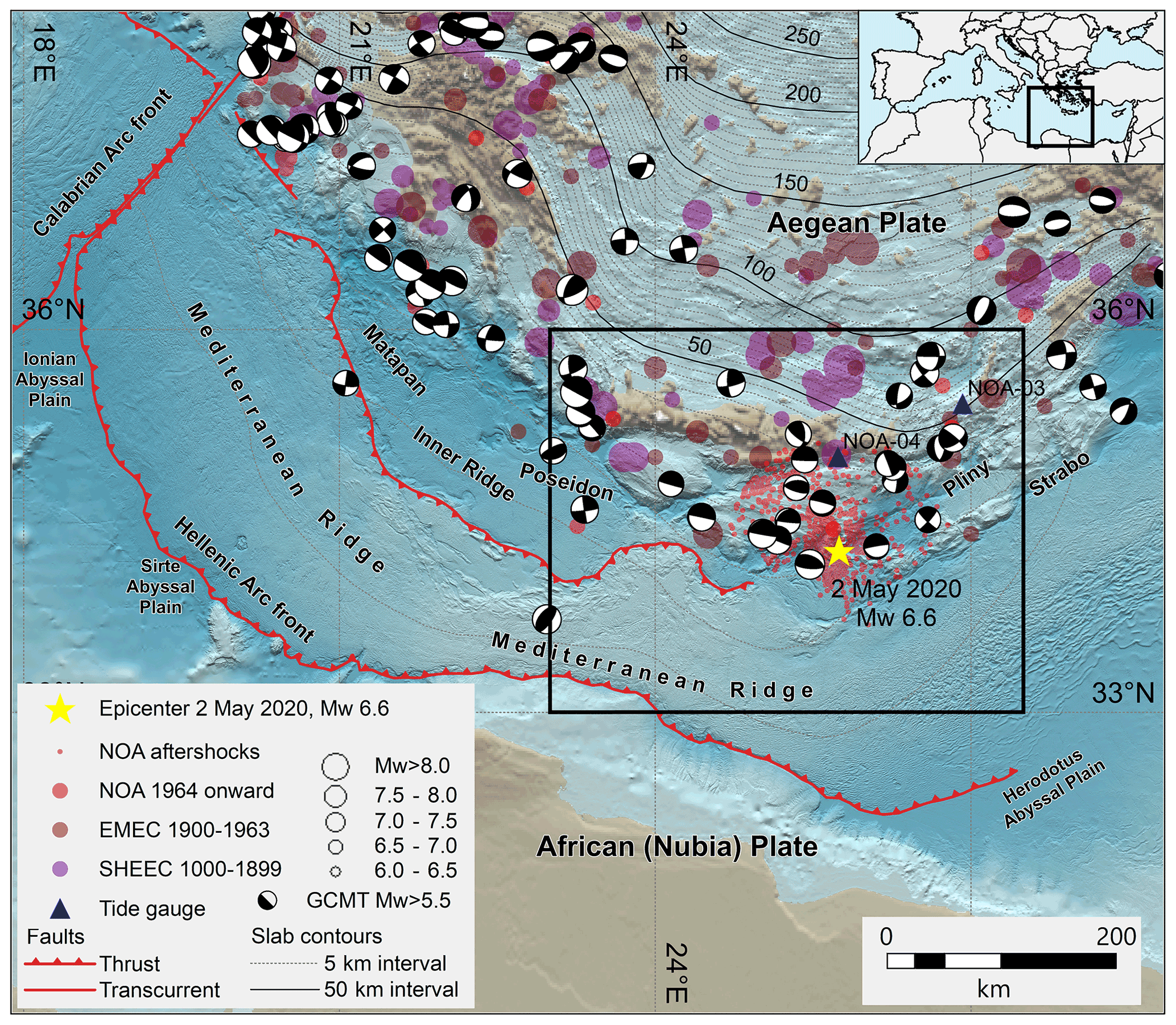
Figure 1Main seismotectonic elements of the Hellenic Arc subduction zone (HASZ). The seismicity is derived by the SHEEC-EMEC (Grünthal and Wahlström, 2012; Stucchi et al., 2013) and NOA (http://www.gein.noa.gr/en/seismicity/earthquake-catalogs, last access: 15 January 2021) earthquake catalogues. Focal mechanisms are from the Global Centroid Moment Tensors database (GCMT; Dziewonski et al., 1981; Ekström et al., 2012). The slab depth contours are resampled from the European database of Seismogenic Faults (EDSF) (Basili et al., 2013). The topography–bathymetry is obtained by splicing the ETOPO1 Global Relief Model and EMODnet Digital Bathymetry (DTM 2020) (NOAA, 2009; Amante and Eakins, 2009; EMODnet Bathymetry Consortium, 2020). The inset shows the location of this map, and the black rectangle outlines the area shown in Fig. 2a.
We compared the sea level observations at the Ierapetra tide gauge with the synthetic waveforms obtained through numerical tsunami simulations to identify the source that produced the tsunami based on many different sets of fault parameters. In this section, we describe the technical details of our approach.
2.1 Seismic source parameterization
The symmetry of the problem, in terms of source size and position relative to the Ierapetra tide gauge, does not allow us to constrain the size of the fault along strike direction; thus, we adopted a fixed source size. We use a rectangular fault with uniform slip, where length and width were assigned based on earthquake scaling relations (Leonard, 2014) for a fixed moment magnitude Mw=6.6. We also varied position, depth, strike, dip, rake, and slip, testing different combinations of source parameters for a total of 41 310 solutions (Table 1).
The earthquake struck in a region where hypocentral locations are usually poorly constrained (Bocchini et al., 2020). The use of a different number of seismic stations, the type of phases used (namely at local, regional, or teleseismic distances), and the choice of velocity models can lead to a significant discrepancy in hypocentral locations. The centre of the rectangular fault is thus allowed to span different values of latitude, longitude, and depth (Table 1) to consider this variability.
Strike, dip, and rake are explored by regular steps within a range of values that envelope the focal mechanism solutions provided by several agencies (GFZ, USGS, GCMT, IPGP; Fig. 2a). Two classes of nodal planes are explored; one is a north shallow-dipping plane, coherent with the dip direction of the subduction interface in that region, or a splay fault (hereafter called “plane S”), and the other one is a steep south-dipping plane, likely identifying a back-thrust (“plane B”). Some “extreme” values, like a dip larger than 70∘ for plane B or lower than 20∘ for plane S, have been excluded after some preliminary tests, as they were significantly worsening the misfit between synthetic and observed waveforms. Slip is allowed to vary between 0.35 and 1.15 m, with a step of 0.05 m.
Table 1Source parameter variability of the source model dataset for the tsunami simulations. The different sets of focal plane parameters are separated by parentheses (B and S refer to the back-thrust and splay fault solutions). Positions and depths are in reference to the centre of the fault plane.

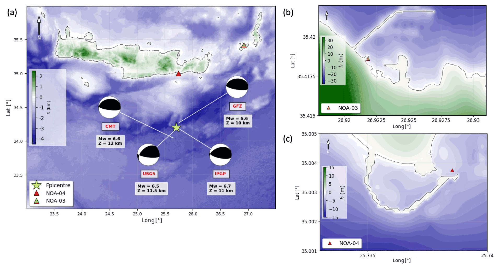
Figure 2(a) Computational domain for the tsunami modelling adopted in this study (see text for details). The yellow star indicates the epicentre, at the centre (34.2∘ N, 25.7∘ E) of its considered variability range. The different bathymetric levels are plotted as black rectangles. The red and orange triangles represent the Ierapetra (NOA-04) and Kasos (NOA-03) tide gauge stations, respectively. The different focal mechanisms used as reference values to let the inversion parameters vary are plotted, each with its own agency label: GEOFON (GFZ, https://geofon.gfz-potsdam.de/, last access: 1 April 2021), United States Geological Survey (USGS, https://earthquake.usgs.gov/, last access: 1 April 2021), Institut de Physique du Globe de Paris (http://geoscope.ipgp.fr/, last access: 1 April 2021), and Global CMT Catalog (https://www.globalcmt.org/, last access: 1 April 2021). (b) High-resolution bathymetry data (10 m spatial resolution) around NOA-03 (Kasos) and (c) NOA-04 (Ierapetra) tide gauges.
2.2 Tide gauge data and tsunami modelling
The tsunami signal recorded by the tide gauges at Ierapetra (NOA-04) and Kasos (NOA-03) was obtained after removing the tidal component from the original waveform (http://www.ioc-sealevelmonitoring.org, last access: 25 February 2021, sampling rate of 1 min) through a LOWESS procedure (e.g. Romano et al., 2015).
Tsunami numerical modelling was performed with the Tsunami-HySEA software, which solves non-linear shallow water equations using a finite volume approach and a nested grid scheme to progressively increase the resolution during the propagation from the source to the tide gauges.
The software has undergone proper benchmarking (Macías et al., 2017) according to the community standards (e.g. Synolakis et al., 2009), also within the framework of the US tsunami hazard programme (http://nws.weather.gov/nthmp/, last access: 20 November 2020). The code is implemented in CUDA (Compute Unified Device Architecture) and runs in multi-GPU architectures, yielding remarkable speedups compared to other CPU-based codes (de la Asunción et al., 2013).
Dispersion effects are not considered in the governing equations and, thus, are not modelled. Nevertheless, we have assumed this approximation to be acceptable because the main tide gauge station (Ierapetra) is located sufficiently close to the source (about 80 km). For such a distance, and for a relatively small source, even if the waveform period is relatively short (∼5 min), we assume the effects due to the dispersion are negligible (see Sandanbata et al., 2021; Heidarzadeh and Gusman, 2021).
To build the bathymetric and topographic grid models for the simulations, we used (1) the European Marine Observation and Data Network (EMODnet) project database (EMODnet DTM version released in 2018, http://portal.emodnet-bathymetry.eu/, last access: 23 April 2021), which has a resolution of about 115 m; (2) the European Digital Elevation Model (EU-DEM), version 1.1 (eu_dem_v11_E50N10), with a resolution of 25 m; and (3) the nautical charts (https://hartis.org/en, last access: 23 April 2021) of Ierapetra harbour (Ierapetra Bay, 1:10 000 scale; Kaloi Limenes Bay, 1:12 500 scale, original version: 1962, with small corrections in the period 1964–2010) and Kasos harbour (Diafani Harbour, 1:5000 scale; Pigadia Bay and Harbour, 1:5000 scale; Emporio Harbour, 1:5000 scale, original version 1998, with small corrections in the period 2000–2020). The computational domain (33–36∘ N, 23–27.5∘ E, Fig. 2a) for tsunami propagation consisted of four levels of nested grids with increasing resolution approaching the Ierapetra and Kasos harbours (640, 160, 40, and 10 m, respectively). The domains of the finest grids are shown in Fig. 2b and c.
The instantaneous seafloor vertical displacement was calculated using Volterra's formulation of elastic dislocation theory applied to a rectangular source embedded in an elastic half-space (Okada, 1992), and the initial velocity field is assumed to be zero everywhere. The initial sea surface elevation was obtained by applying a low-pass filter to reproduce the water column attenuation; the filter has a trend of the type , where “k” is the wavenumber and “h” is the average water depth (Kajiura, 1963).
We performed 2430 simulations exploring all the source parameters (Table 1) except for the slip, which is fixed in all runs to 1 m to obtain Green's functions. For all of these scenarios, we simulated 1 h of propagation after the earthquake origin time (hereinafter OT) for the Ierapetra station and 1 h and 30 min of propagation for the Kasos station. These simulation lengths allowed us to have about 50 min of tsunami signal at both gauges, which is more than enough to include the first tsunami oscillations (∼30 min) that carry the information on the source and are used for the inversion (see Sect. 2.3). Time histories of the tsunami waves were calculated at the wet points of the computational grid closest to the Ierapetra and Kasos station coordinates (see Fig. 2). The synthetic signals were resampled to the observed data sampling rate (one per minute) through a linear interpolation. We assumed linearity between the slip amount and the tsunami to obtain the scenarios for different slip values. The assumption of slip linearity was preliminarily tested and verified (results are shown in the Supplement).
Thus, we multiplied each of the computed marigrams by all the 17 slip values, for a total of 41 310 tsunami realizations.
2.3 Inversion
To retrieve the fault parameters and the coseismic slip simultaneously, we solved a nonlinear inverse problem. Since the number of sources in our ensemble is not very large, we opted for a systematic search of the parameters' space.
The comparison between the synthetic and the observed waveforms is carried out in the time domain. The misfit between the two waveforms is evaluated through a cost function frequently used to compare tsunami signals in source inversions (e.g. Romano et al., 2020):
In Eq. (1) η(t) and η0(t) are the synthetic and the observed waveforms, respectively; ti and tf are the lower and upper limits of the considered time window; and T is a time shift. The cost function considers both the amplitude and the shape of a waveform; it is more robust than a least-squares misfit, whose solutions are very sensitive to a small number of large errors in the dataset (Tarantola, 1987). For each combination of the source parameters, the cost function is minimized with respect to time shift values between −5 and 5 min, with 1 min steps. The arrival time optimization is used to overcome the often found time alignment mismatch between the observed and modelled tsunami waveforms, with the latter generally arriving earlier. This approach was introduced by Romano et al. (2016), and the details are discussed further in Romano et al. (2020).
Kasos tide gauge is in the far field of the tsunami source (see Fig. 2) and its signal-to-noise ratio is so low. After several preliminary tests, where both the tide gauge waveforms were inverted, we observed that the Kasos tide gauge was not significantly sensitive to constrain the tsunami source of the 2020 Cretan passage event. Therefore, we decided to use only the signal recorded at Ierapetra.
Time window of [5, 30] min after the earthquake OT is chosen. This choice was made to include the first tsunami oscillations, which are mainly driven by the seismic source. The remaining part of the records is not used for the inversion, because it is highly probable that other factors, such as the local propagation and the port structure, start to control the shape of the signal (Romano et al., 2016; Cirella et al., 2020). To quantify the relative importance of these factors, the cost function is also evaluated in the 25 min following the considered interval, that is in the time windows [30, 55]. The average of the cost functions (E1 for [5, 30], E2 for [30, 55]) is calculated from the 5 %, 10 %, 50 %, and 100 % of models with the lowest misfit E1 (within the first window used for the inversion) with the observed data. We observe that the ratio significantly decreases when using progressively more models (, 7.9, 3.9, 2.7, respectively). This observation confirms that the information about the source dominates the first intervals used for the inversion.
2.4 Synthetic test
We first investigated the resolution offered by the two stations using as a target source model all possible combinations of the source parameters . These are the same models we explored in the inversion for the real case. For each of them we calculated the corresponding synthetic target waveform and corrupted it by adding a Gaussian random noise with a variance corresponding to the 10 % of the clean waveform amplitude variance. A random time shift between −5 and 5 min is added to mimic the typically observed time mismatch between the observed and the predicted tsunami signals.
All the waveforms f(A) derived from all the possible source models are tested against each of these noisy and shifted target waveforms fT(A) using Eq. (1). We then defined the distance between two different models as
where ai= (strike, dip, rake, slip, depth, long, lat)i and aj= (strike, dip, rake, slip, depth, long, lat)j are the parameters associated with the ith (jth) combination ( is the square root of the sum of the squares of the parameters), and M (equal 7) is the number of free parameters.
For each target model ai, the distance d is evaluated with respect to
-
the best model abest, whose f(abest) presents the lowest cost function, and
-
the average model awm evaluated as a weighted mean over the first 5 % of the models with the lowest cost function, where the weights are chosen as the reciprocal of the cost function.
The result confirms that the tsunami data constrain the seismic source process well. In most cases, the target parameters correspond to those of the model, which minimizes the cost function (Fig. 3a and c). Hence, the target focal plane is correctly identified. The few cases showing a high value of the distance occur when the algorithm does not recognize if the target is a back-thrust or a splay fault.
On the one hand, when using the average model, the distance between the models almost never vanishes (Fig. 3b and d), meaning that the target's parameters are not perfectly reproduced, as expected for an average model. On the other hand, the averaging process has the power to make the distribution smoother and unimodal and to eliminate or diminish the number of occurrences corresponding to a high distance. So, choosing the average over the best models may protect us from overfitting. Figure 3e shows that the B plane (a back-thrust) is much better spotted than the S one (the splay) by the best models; when using the average model, the difference in the “specificity” of the cost function is slightly reduced but still present (Fig. 3f).
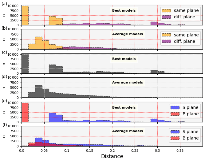
Figure 3Distributions of the parameter distance for the best (panels a, c, e) and average models (panels b, d, f). Panels (a) and (b) separate the models for which the target model focal mechanism is reproduced or not. Panels (c) and (d) report all the models together. Panels (e) and (f) separate the target models associated with the B (red) or S (blue) focal plane solutions.
We performed the inversion using the observations at Ierapetra, the only near-source sea level recording available. The distribution of the cost function values for all the investigated models is shown in Fig. 4. Figure 4a separately displays the cost function values obtained for the two focal solutions. Overall, the cost functions of the B plane are slightly lower than those of the S plane. However, the left portions of the distributions, that is the ones containing the models with the lowest misfit with respect to the observed marigrams, are almost overlapped. The same tendency can be seen in Fig. 4b where the distribution has a slightly bimodal character with the two modes corresponding to the S and B planes.
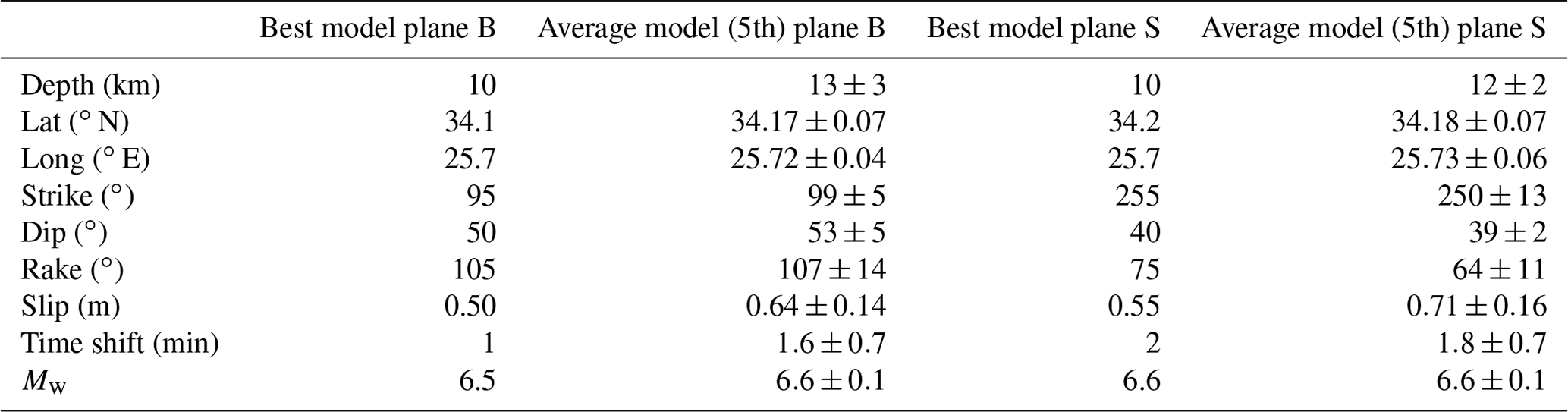
Based on the resolution test results presented in the synthetic test, we evaluated the weighted average of the models included in the 5th percentile of the cost function distribution for each focal solution (those to the left of the dashed lines in Fig. 4a). We used as a weight the inverse of the cost function. Both the best and average models, as well as the associated errors obtained as weighted standard deviations, are reported in Table 2.
The average models, along with the associated errors, may indicate that the best model is “overfitting” the data. This happens, for example, when the best and average models are very different or when the uncertainties are very large. Standard deviations give a measure of the uncertainties in the estimation of the corresponding parameter. Smaller values of the standard deviation denote a parameter's better resolution (Mosegaard and Tarantola, 1995; Sambridge and Mosegaard, 2002; Piatanesi and Lorito, 2007).
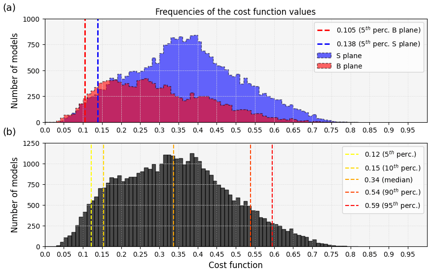
Figure 4(a) Cost function distribution for the back-thrust (red) and the splay (blue) models; the vertical dashed lines indicate the 5th percentiles for each of the two focal solutions. (b) Histogram of the cost function values for all the models considered. The vertical dashed lines represent the 5th, 10th, 50th (median), 90th, and 95th percentiles.
With only a few exceptions, all the best model parameters fall within the range of 1 standard deviation from the average model. For both focal solutions, the slip of the best models is much smaller than the average one and does not fall within the uncertainty limits.
The S plane solutions are centred about 10 km north of the B planes, slightly closer to the southern coast of Crete. Coherently, the predicted tsunami arrives earlier (i.e. the estimated time shift is bigger) with respect to the waves resulting from the B plane solutions. The rake angle, for both B and S planes, presents a large dispersion. The same can be said for the strike associated with the S plane. On the other hand, the dip appears to be better constrained.
Table 2Best and average model extracted from the models with the smallest cost functions within the 5th percentile. The percentiles refer to the B and S planes separately (i.e. the models at the left of the red and blue vertical dashed lines in Fig. 4a, respectively). B plane refers to the back-thrust solution dipping south; S plane refers to the splay fault dipping north. Lat, Long, and Depth refer to the centre of the fault.
Figures 5–7 help to visualize the parameter variability and how the best source models are characterized. The marginal (Fig. 5) and the joint distributions (Figs. 6 and 7) are provided for the two planes. Marginal and joint distributions provide an additional measure of the uncertainties. Narrower distributions suggest that the corresponding parameters are better resolved than those characterized by broader ones.
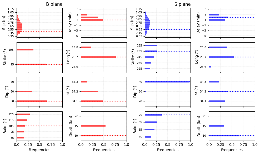
Figure 5Marginal distributions for each of the inverted parameters, considering the first 5 % of B (first and second columns) and S (third and fourth columns) plane models, those at the left of the red and blue vertical lines in Fig. 3a. The red and blue horizontal dotted lines mark the best models for the B and S planes, respectively.
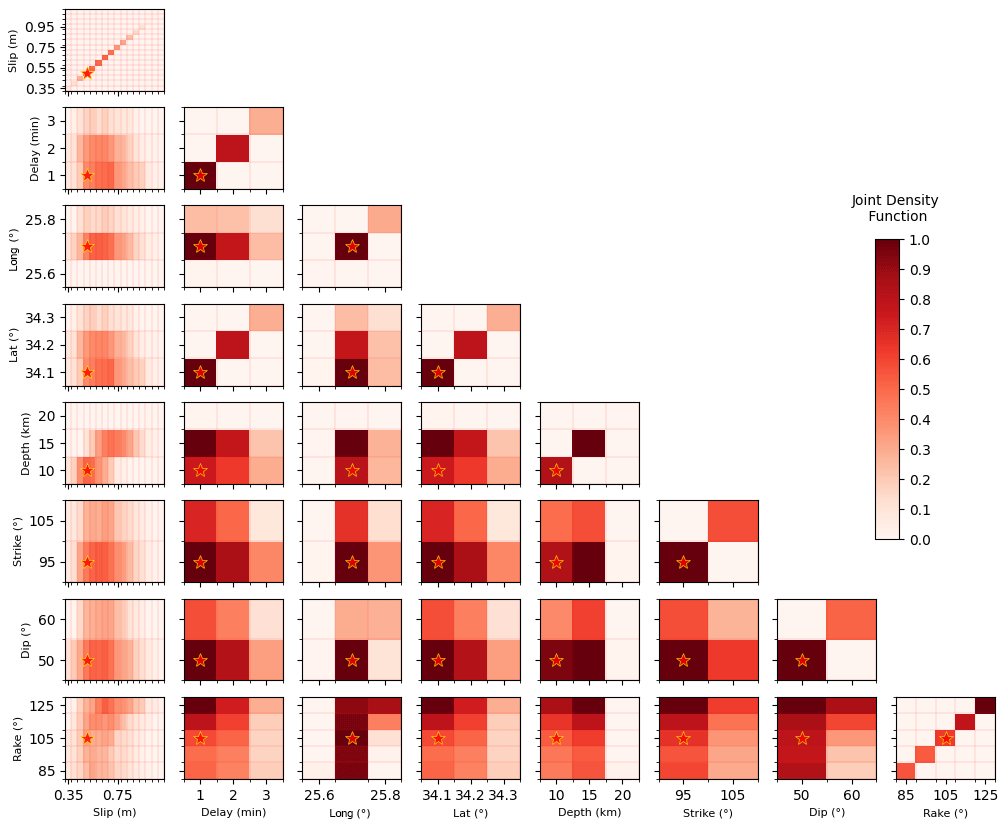
Figure 6Joint density distribution for each couple of the back-thrust source's parameters, considering the first 5 % of B plane models, those at the left of the red vertical line in Fig. 3a. The red star identifies the best model.
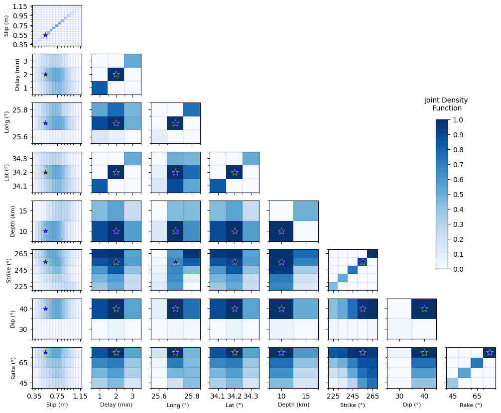
Figure 7Joint density distribution for each couple of the splay source's parameters, considering the first 5 % of S plane models, those at the left of the blue vertical line in Fig. 3a. The blue star identifies the best model.
The strike angle for plane B and the dip angle for plane S show a strongly “preferred” value (diagonals of Figs. 6 and 7). The rake angle does not show a real preferential value: evidently, we do not have enough precision to discriminate at this level of resolution. Plane B solutions are characterized by a larger depth dispersion and by a higher average depth value. However, the depth of 20 km almost never occurs, suggesting the occurrence of a shallow event. The slip shows a “bell-shaped” distribution with a peak at 0.60 and 0.70 m for the B and S planes, respectively, and significant occurrences in the range 0.45–0.90; the best source slip is lower than the average, for both plane S and B. S plane solutions are characterized by a slightly higher slip than B plane solutions. There is a correlation between the slip and depth values: deeper solutions consistently feature a larger slip. In this case, a lighter correlation also exists between slip and latitude: events further south have a slightly greater slip, especially for B solutions. With regards to the hypocentre determination, establishing a univocal position is not obvious, also because the delay adds a trade-off in constraining the hypocentre. Consequently, the longitude is better constrained than the latitude since the latter is more strongly correlated with the arrival time given the relative position of the tide gauges (both to the north) with respect to the source. The preferred longitude is 25.7∘ E, with fewer occurrences a little further east and almost none further west.
There surely can be other parameter combinations (length, width) that could fit the data equally well because of the problem symmetry discussed in Sect. 2.1. But, for the reasons mentioned above, we decided to fix the fault length and width, using the Leonard relationship because it is derived from the seismic moment and suitable for a crustal event.
The comparison between the observed data and the synthetic ones generated with both the best and the average source models at Ierapetra and Kasos tide gauges is shown in Fig. 8; those corresponding to the two planes B (Fig. 8a and e) and S (Fig. 8c and g) are plotted separately. Both synthetic signals reproduce the first oscillations (covering about 15 min) quite well. For what concerns the peak at minute 28, the average signals tend to be lower.
It is interesting to note a possible “clipping” of the negative peak of the signal at about minute 27 caused by the insufficient sampling frequency.
In terms of wave fitting, the comparison between the data and the predictions of the average models is only slightly worse than that found with the best model. Apart from the coseismic slip value, the best and average models are similar, especially for the focal mechanism parameters (see Table 2); hence, both the models can be chosen to represent the best sources' ensembles.
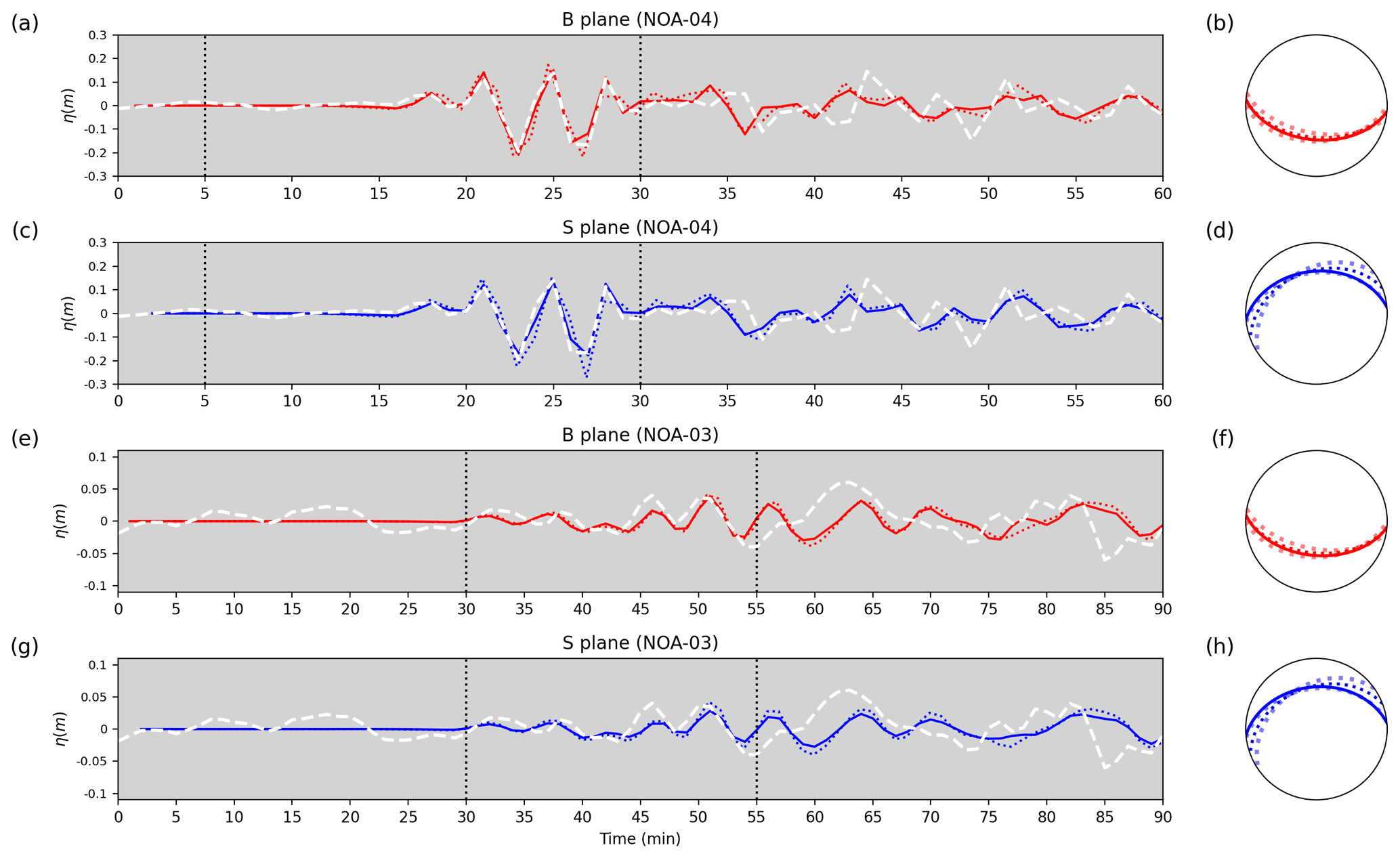
Figure 8Best (solid lines) and average (dotted lines) marigrams obtained at the two stations. Panels (a) and (c) refer to the Ierapetra tide gauge (NOA-04) while (e) and (g) refer to the Kasos one (NOA-03). The white dashed line is the observed water elevation at each tide gauge. B plane (in red) refers to the back-thrust solution dipping south; S plane (in blue) refers to the splay fault dipping north. The vertical dotted lines indicate the limits of the time window used for the inversion. On the right of each marigram plot the stereonets (lower hemisphere) show the fault orientations corresponding to the best signal (solid line) and the average one (dotted line) with the variability derived from the standard deviations of Table 2.
The signals belonging to the 5th, 10th, 50th, and 100th percentiles of the cost function are shown in Fig. 9 to provide a better idea of what a certain cost function implies in terms of waveform fitting with respect to the observed data. Significant discrepancies start to appear when including the models in the 10th percentile and beyond, confirming that all the models with a lower cost function may be equally reasonable solutions.
The synthetic marigrams at Ierapetra reproduce the observed tsunami waveforms for the first cycles of the signal, those carrying most of the source-related information quite well. As discussed above, the agreement worsens as time progresses due to the possibility of not well-modelled propagation complexity around the tide gauge. After roughly half an hour from the tsunami first arrival, there is a larger and larger deviation between the synthetic and the observed marigrams (Fig. 8).
Overall, the results do not conclusively indicate that one focal plane should be preferred over another, and both solutions remain possible.
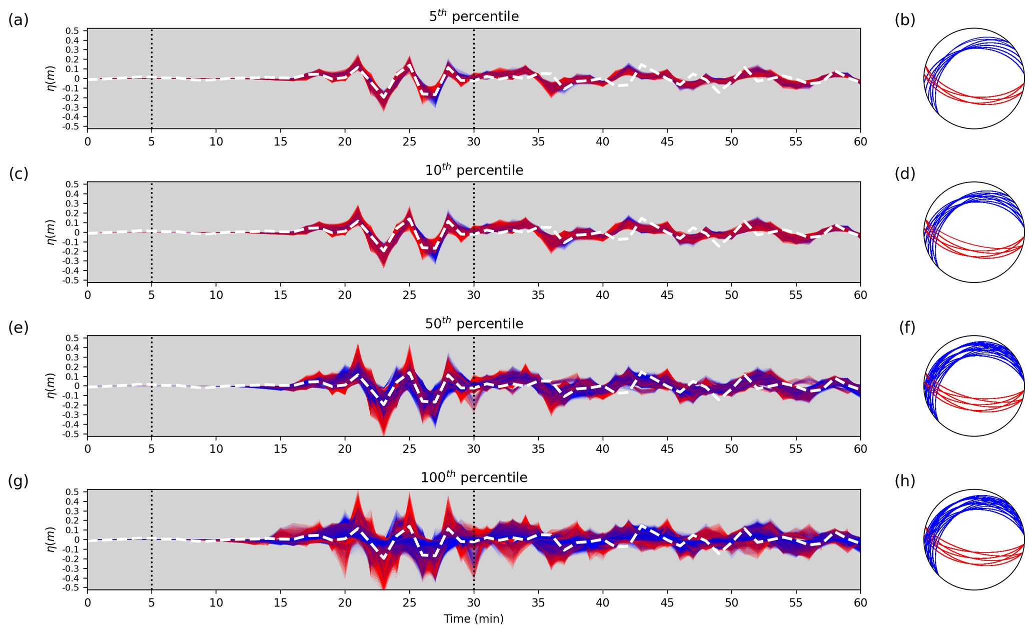
Figure 9From top to bottom, the left-hand-side panels (a, c, e, g) show the marigrams of the events, ordered by cost function value, corresponding to the 5th, 10th, 50th, and 100th percentiles. The white dashed line is the observed water elevation at the Ierapetra tide gauge (NOA-04). The vertical dotted lines indicate the limits of the time window used for the inversion. The stereonets (lower hemisphere) on the right-hand side (b, d, f, h) show the fault plane variability corresponding to the synthetic waveforms. Red and blue refer to plane B (back-thrust solutions) and plane S (splay fault solutions), respectively, for both waveforms and fault planes.
We constrained the source model of the 2020 Cretan Passage earthquake (Mw 6.6) by comparing the sea level observations at the Ierapetra tide gauge with the synthetic tsunami waveforms.
We could use only one tsunami record (not too distant from the source) in the near-field domain to estimate the tsunami source of the 2020 event, whereas we used an additional tide gauge (Kasos) positioned in the far field of the tsunami source as an independent verification of the results. The availability of more instruments would be advantageous for both real-time operations and event characterization. Moreover, a better characterization of harbour response and the implementation in the future of high-resolution in-harbour propagation could be important, particularly considering that deep-sea instruments are nearly absent in the Mediterranean Sea.
We compared the waveforms generated with our solutions with those we simulated using two different source models already published for the 2020 Cretan Passage tsunami: the one presented by Wang et al. (2020; “W” model hereafter), who use the event as a test case for a hypothetical offshore bottom pressure gauge network around Crete, to assist tsunami early warning through real data assimilation, and the Heidarzadeh and Gusman (2021) model (“HG” model hereafter), obtained by inversion of the same tsunami dataset we used in this study.
Figure 10 displays the marigrams calculated with our preferred models together with the waveforms generated by the W and HG models. The W waveform tends to overestimate the observed signal, at both Ierapetra and Kasos tide gauges. The HG waveform reproduces the observed signal at the Ierapetra station well, while it overestimates the signal around minute 50 at Kasos. The cost functions associated with the four models, evaluated as described in Sect. 2, are 0.097, 0.104, 0.583, and 0.253 for our B and S planes and for the W and HG models, respectively. Using these values, and assuming a rigidity of 33 GPa, consistent with the scaling relationships of Leonard (2014), the seismic moment associated with the four source models is 6.63, 7.29, 11.9, and 11.1 (×1018) Nm, corresponding to Mw 6.5, 6.6, 6.7, and 6.7, respectively.
The W model, whose waveform presents the largest misfit, consists of a single fault (20 km×12 km) with a uniform slip of 1.5 m. The epicentre is at 34.205∘ N, 25.712∘ E, and the top depth of the fault is 11.5 km; strike, dip, and rake angles are 229, 31, and 46∘, respectively. These parameters are based on the W-phase focal mechanism solution of the USGS. The slip value is significantly larger than in our preferred models, and it can explain the overestimation. When the same source is used by Wang et al. (2020; see their Fig. 9), the agreement between the synthetic and observed waveforms is better. However, Wang et al. (2020) used a bathymetric grid with a resolution of 30 arcsec (∼925 m), while we used a nested grid approach with a resolution up to 10 m around the tide gauge positions (see Sect. 2). This likely guarantees a better convergence of the numerical simulation of the relatively short wavelengths characterizing this tsunami and explains the difference. When using a lower resolution, the waveforms can only be reproduced by artificially increasing the fault slip. The role of accurate bathymetry is of fundamental importance to ensure accurate tsunami simulations for source characterization as well.
The HG model, with assigned location and focal mechanism (reported in the Introduction), presents a source dimension of 40×30 km and a heterogeneous slip distribution with a maximum slip of 0.64 m and an average slip of 0.28 m. In this case, high-resolution modelling is used around the tide gauges as well. The slip value of our sources is much larger than their average, but associated with a smaller fault (see Table 1). The overall higher cost function value for the HG model retrieved with our setup can be explained by the fact that the inversion time windows are 13 and 10 min for the Ierapetra and Kasos tide gauges, respectively, much shorter than the one used in this study (Sect. 2).

Figure 10Waveforms obtained at the Ierapetra NOA-04 (a) and Kasos NOA-03 (b) tide gauges by the best source models of the back-thrust solution (the B plane in red), the best of the splay fault solution (the S plane in blue), the fault defined by Wang et al. (2020), and the fault defined by Heidarzadeh and Gusman (2021). The vertical dotted lines indicate the limits of the time window used for the inversion.
Starting from the available focal mechanisms, we explored two thrust faulting solutions (Fig. 11), a north-dipping reverse splay fault (plane S) and a south-dipping back-thrust fault (plane B). We found a slightly better agreement for the waveforms corresponding to the B plane with respect to those of the S plane (Fig. 4). However, this difference is not big enough to draw a strong conclusion concerning the causative fault of this earthquake.
Despite this ambiguity between the two fault planes (S and B), important considerations still emerge from this study. Both solutions seem shallow enough to indicate that the earthquake was embedded within the inner parts of the HASZ accretionary wedge, thus excluding either a subduction interface or intraslab earthquake. In particular, the strike of the B plane and the dip of the S plane contribute to excluding a subduction interface earthquake.
From the geological viewpoint, plane B could represent a back-thrust fault accommodating the contraction of the inner parts of the Mediterranean Ridge against the Cretan backstop. This southeastern Cretan margin is surrounded by the double Pliny and Strabo trench system, which have been related to back-thrust fault activity (Camerlenghi et al., 1992; Leite and Mascle, 1982; Chaumillon and Mascle, 1997). Back-thrusting is considered to be the cause of the formation of a topographic escarpment separating the wedge from the Inner Ridge backstop (Kopf et al., 2003). The plane S could represent the reactivation of one of the thrusts, marking the advancement of the deformation front within the accretionary wedge above the main decollement or a splay fault emanating directly from the subduction interface.
In either case, the orientation of the fault plane and the slip direction are compatible with the long-term kinematic indicators. Within the region of the HASZ where the Cretan Passage earthquake occurred, in fact, the average direction of convergence is ∼200–220∘ from GPS velocity data (Reilinger et al., 2006; Floyd et al., 2010; Nocquet, 2012), and the azimuth of the maximum horizontal stress (SHmax) is 0–20∘ (Carafa and Barba, 2013). The splay fault S features a small left-lateral slip component, which is consistent with the increasingly oblique convergence in the eastern branch of the HASZ (Bohnhoff et al., 2005; Yolsal-Çevikbilen and Taymaz, 2012).
The combination of the shallow depth and the high dip angle plays a key role in determining the tsunamigenic potential associated with the fault. The steeper dip angle and the shallower depth tend to produce a vertical deformation whose tsunamigenic potential is more pronounced than that induced by the very low angle interface earthquakes of similar magnitude. Note, however, that the dip angle of the two proposed solutions is higher than those derived from seismic reflection profiles for these types of thrust faults in the region (Kopf et al., 2003).
For example, the moderate earthquake of Mw=6.45, which occurred on 1 July 2009 (Bocchini et al., 2020), was the cause of a local tsunami because it ruptured in the overriding crust as for the 2020 Cretan Passage earthquake. Conversely, other larger earthquakes occurred nearby, apparently without generating a tsunami. Just focusing on the portion of the Hellenic Trench south of Crete, this is, for example, the case of the Ms 7, 17 December 1952 earthquake that occurred at a depth of about 25 km (Papazachos, 1996) and the Ms 6.5, 4 May 1972 earthquake that occurred at ∼40 km depth (Kiratzi and Langston, 1989).
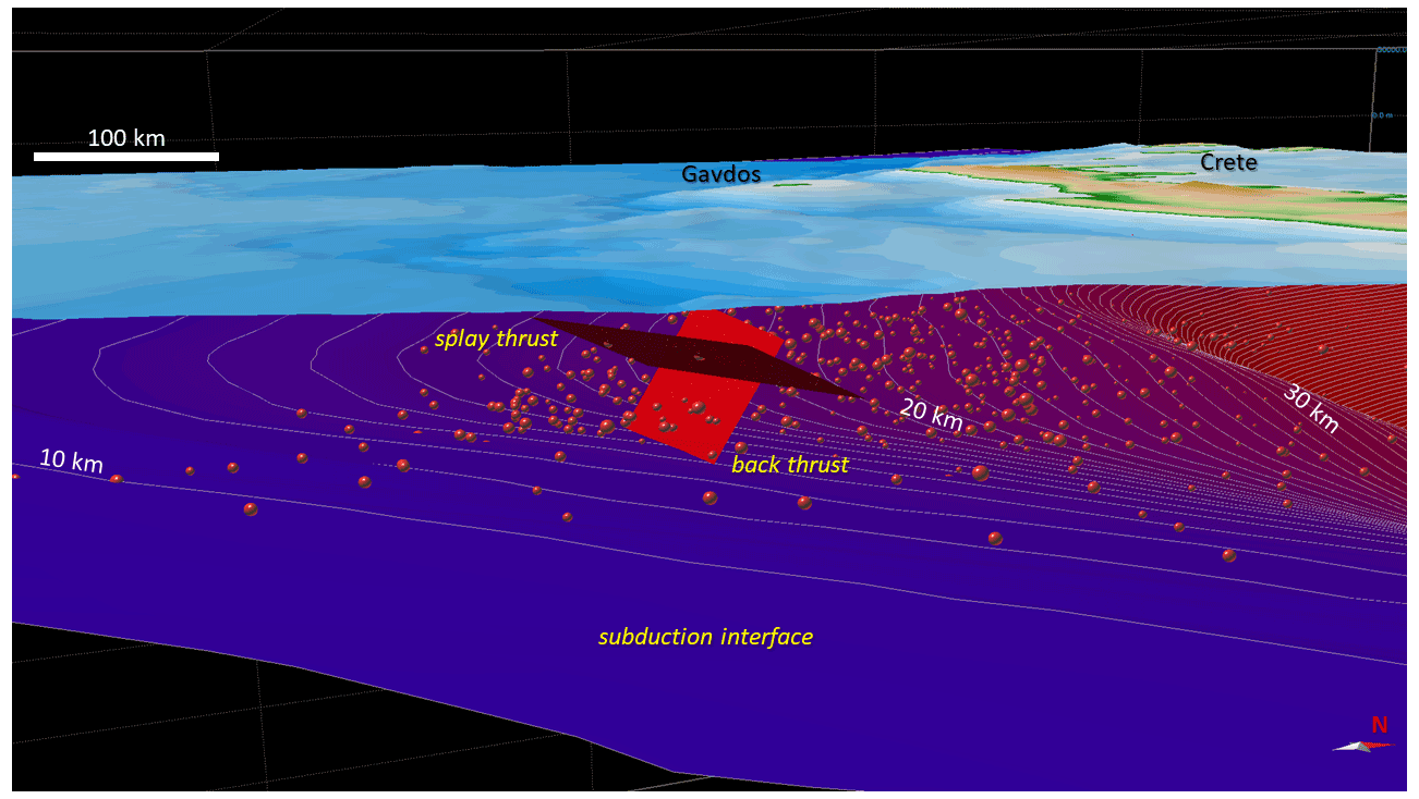
Figure 11Oblique view, looking westward, of the fault planes obtained in this study and their relation with the subduction interface shown by depth contours (white lines) and the aftershock seismicity (red spheres) until 18 April 2021.
We investigated the seismic fault structure and the rupture characteristics of the Mw 6.6, 2 May 2020 Cretan Passage earthquake through tsunami data inverse modelling. Our results confirm the indication from moment tensor solutions that this was a shallow crustal event with a reverse mechanism within the accretionary wedge rather than on the Hellenic Arc subduction interface.
Using just two marigrams, only one of which is in the near field with respect to the seismic source, we could highlight important characteristics of this earthquake, especially from a tsunami genesis perspective, although the adopted method and the limited data available did not prove sufficient to isolate the main focal plane. The sea level heights recorded at Ierapetra tide gauge identify two possible ruptures: a steeply sloping reverse splay fault and a back-thrust rupture dipping south, with a more prominent dip angle. The a posteriori appraisal of the ensemble of models tested allows for a slight preference for the south-dipping back-thrust over the splay fault.
Nevertheless, both are high-angle reverse faults in the upper plate above the plate interface with a tsunamigenic potential higher than that of interplate earthquakes of similar or even slightly larger moment magnitude.
This is important for seismic and tsunami hazard assessment, since the presence of shallow crustal ruptures should not be overlooked in an area where subduction interface (interplate) events are also possible. Note that, for example, the recent NEAMTHM18 tsunami hazard model considered the possibility of crustal faults rupturing everywhere in the overriding plate (Basili et al., 2021).
Although the tsunami did not cause damages or victims, the event represents yet another testimony of how such events are frequent and typical in the Mediterranean and, particularly, along the Hellenic Arc. In addition to this, the near-source nature of the event should be emphasized. Despite the improvements and developments carried out by the NEAMTWS Tsunami Service Providers in recent years, which have proven to be capable of issuing tsunami messages within 10 min after the earthquake origin time (Amato et al., 2021), the early tsunami arrival (tenths of minutes or less) at the closest coasts leaves very little time for warning, which is probably the case in many regions in the world. Then, together with an efficient warning system, education, awareness, and preparation remain by far the most cost-effective investments for local tsunamis (Imamura et al., 2019). The 2020 Cretan Passage earthquake is another reminder of the tsunami risk in the Mediterranean Sea, but also of the fact that it is extremely appropriate to promptly react to felt shaking, since moderate earthquakes that are shallow and occur on steep faults may also generate a significant and dangerous tsunami.
The sea level data used in the current study were obtained from https://webcritech.jrc.ec.europa.eu/TAD_server/Device/106 (last access: 23 April 2021; TAD SERVER, 2021). The different focal mechanisms used as reference values were obtained from GFZ (https://doi.org/10.14470/TR560404; GEOFON Data Centre, 1993), United States Geological Survey (USGS, https://earthquake.usgs.gov/earthquakes/eventpage/us700098qd/origin/detail?source=us&code=us700098qd, last access: 1 April 2021; USGS, 2021), Institut de Physique du Globe de Paris (https://doi.org/10.18715/GEOSCOPE.G; GEOSCOPE, 2021), and Global CMT Catalog (https://www.globalcmt.org/cgi-bin/globalcmt-cgi-bin/CMT5/form?itype=ymd&yr=2020&mo=5&day=2&oyr=1976&omo=1&oday=1&jyr=1976&jday=1&ojyr=1976&ojday=1&otype=nd&nday=1&lmw=5&umw=7&lms=0&ums=10&lmb=0&umb=10&llat=-90&ulat=90&llon=-180&ulon=180&lhd=0&uhd=1000<s=-9999&uts=9999&lpe1=0&upe1=90&lpe2=0&upe2=90&list=0; (last access: 1 April 2021; CMT, 2021). The bathymetric and topographic grid models for the simulations were realized using the European Marine Observation and Data Network (EMODnet) project database (https://doi.org/10.12770/bb6a87dd-e579-4036-abe1-e649cea9881a; EMODnet Bathymetry Consortium, 2021) and the European Digital Elevation Model (EU-DEM, 2017, https://www.eea.europa.eu/data-and-maps/data/eu-dem, last access: 23 April 2021) and two nautical charts (https://hartis.org/en/p/1188/Nautical_Charts/South_Aegean/Crete/Ierapetra_-_Kaloi_Limenes_Bays_Nautical_Chart?search=ierapetra, https://hartis.org/en/p/1190/Nautical_Charts/South_Aegean/Dodecanese/Bays_and_Harbours_of_Kassos_and_Karpathos_Islands_Nautical_Chart, last access: 23 April 2021).
The supplement related to this article is available online at: https://doi.org/10.5194/nhess-21-3713-2021-supplement.
EB, SL, AP, and FR were involved in all of the phases of this study. RB contributed to the geological interpretation of the data, the discussion of results, the realization of some figures, and paper writing. BB contributed to create the computational grids for the numerical tsunami simulations. MV contributed to the numerical tsunami simulations and discussion of results. HBB, RT, and AA contributed to the discussion of results. All authors reviewed the final paper.
The contact author has declared that neither they nor their co-authors have any competing interests.
Publisher's note: Copernicus Publications remains neutral with regard to jurisdictional claims in published maps and institutional affiliations.
This article is part of the special issue “Tsunamis: from source processes to coastal hazard and warning”. It is not associated with a conference.
Roberto Basili acknowledges the resources made available by the SISMOLAB-3D at INGV. The authors would like to express their thanks to the referees for their careful reading and valuable comments.
The research reported in this work was supported by OGS and CINECA under HPC-TRES programme (award no. 2020-01) and co-funded by the Italian flagship project RITMARE.
This paper was edited by Filippos Vallianatos and reviewed by Gerasimos Papadopoulos and one anonymous referee.
Amante, C. and Eakins, B. W.: ETOPO1 1 arc-minute global relief model: procedures, data sources and analysis, NOAA technical memorandum NESDIS NGDC-24. National Geophysical Data Center, NOAA, https://doi.org/10.7289/V5C8276M (last access: May 2020), 2009.
Amato, A., Avallone, A., Basili, R., Bernardi, F., Brizuela, B., Graziani, L., Herrero, A., Lorenzino, M. C., Lorito, S., Mele, F. M., Michelini, A., Piatanesi, A., Pintore, S., Romano, F., Selva, J., Stramondo, S., Tonini, R., and Volpe, M.: From Seismic Monitoring to Tsunami Warning in the Mediterranean Sea, Seism. Res. Lett., 92, 1796–1816, https://doi.org/10.1785/0220200437, 2021.
Ambraseys, N.: Earthquakes in the Mediterranean and Middle East: A Multidisciplinary Study of Seismicity up to 1900. Cambridge University Press, Cambridge, UK, https://doi.org/10.1017/CBO9781139195430, 947 pp., 2009.
Basili, R., Kastelic, V., Demircioglu, M. B., Garcia Moreno, D., Nemser, E. S., Petricca, P., Sboras, S. P., Besana-Ostman, G. M., Cabral, J., Camelbeeck, T., Caputo, R., Danciu, L., Domaç, H., Fonseca, J. F. de B. D., García-Mayordomo, J., Giardini, D., Glavatovic, B., Gulen, L., Ince, Y., Pavlides, S., Sesetyan, K., Tarabusi, G., Tiberti, M. M., Utkucu, M., Valensise, G., Vanneste, K., Vilanova, S. P., and Wössner, J.: European Database of Seismogenic Faults (EDSF) compiled in the framework of Project SHARE,, https://doi.org/10.6092/INGV.IT-SHARE-EDSF (last access: 31 May 2021), 2013.
Basili, R., Brizuela, B., Herrero, A., Iqbal, S., Lorito, S., Maesano, F. E., Murphy, S., Perfetti, P., Romano, F., Scala, A., Selva, J., Taroni, M., Tiberti, M. M., Thio, H. K., Tonini, R., Volpe, M., Glimsdal, S., Harbitz, C. B., Løvholt, F., Baptista, M. A., Carrilho, F., Matias, L. M., Omira, R., Babeyko, A., Hoechner, A., Gürbüz, M., Pekcan, O., Yalçıner, A., Canals, M., Lastras, G., Agalos, A., Papadopoulos, G., Triantafyllou, I., Benchekroun, S., Agrebi Jaouadi, H., Ben Abdallah, S., Bouallegue, A., Hamdi, H., Oueslati, F., Amato, A., Armigliato, A., Behrens, J., Davies, G., Di Bucci, D., Dolce, M., Geist, E., Gonzalez Vida, J. M., González, M., Macías Sánchez, J., Meletti, C., Ozer Sozdinler, C., Pagani, M., Parsons, T., Polet, J., Power, W., Sørensen, M., and Zaytsev, A.: The Making of the NEAM Tsunami Hazard Model 2018 (NEAMTHM18), Front. Earth Sci., 8, 753, https://doi.org/10.3389/feart.2020.616594, 2021.
Bocchini, G. M., Novikova, T., Papadopoulos, G. A., Agalos, A., Mouzakiotis, E., Karastathis, V., and Voulgaris, N.: Tsunami Potential of Moderate Earthquakes: The July 1, 2009 Earthquake (Mw 6.45) and its Associated Local Tsunami in the Hellenic Arc, Pure Appl. Geophys., 177, 1315–1333, https://doi.org/10.1007/s00024-019-02246-9, 2020.
Bohnhoff, M., Harjes, H.-P., and Meier, T.: Deformation and stress regimes in the Hellenic subduction zone from focal Mechanisms, J. Seismol., 9, 341–366, https://doi.org/10.1007/s10950-005-8720-5, 2005.
Camerlenghi, A., Cita, M. B., Hieke, W., and Ricchiuto, T.: Geological evidence for mud diapirism on the Mediterranean Ridge accretionary complex, Earth Planet. Sci. Lett., 109, 493–504, https://doi.org/10.1016/0012-821X(92)90109-9, 1992.
Carafa, M. M. C. and Barba, S.: The stress field in Europe: optimal orientations with confidence limits, Geophys. J. Int., 193, 531–548, https://doi.org/10.1093/gji/ggt024, 2013.
Chamot-Rooke, N., Rabaute, A., and Kreemer, C.: Western Mediterranean Ridge mud belt correlates with active shear strain at the prism-backstop geological contact, Geology, 33, 861–864, https://doi.org/10.1130/G21469.1, 2005.
Chaumillon, E. and Mascle, J.: From foreland to forearc domains: New multichannel seismic reflection survey of the Mediterranean ridge accretionary complex (Eastern Mediterranean), Marine Geol., 138, 237–259, https://doi.org/10.1016/S0025-3227(97)00002-9, 1997.
Cirella, A., Romano, F., Avallone, A., Piatanesi, A., Briole, P., Ganas, A., Theodoulidis, N., Chousianitis, K., Volpe, M., Bozionellos, G., Selvaggi, G., and Lorito, S.: The 2018 Mw 6.8 Zakynthos (Ionian Sea, Greece) earthquake: seismic source and local tsunami characterization, Geophys. J. Int., 221, 1043–1054, https://doi.org/10.1093/gji/ggaa053, 2020.
CMT: Global CMT Catalog, CMT [data set], available at: https://www.globalcmt.org/cgi-bin/globalcmt-cgi-bin/CMT5/form?itype=ymd&yr=2020&mo=5&day=2&oyr=1976&omo=1&oday=1&jyr=1976&jday=1&ojyr=1976&ojday=1&otype=nd&nday=1&lmw=5&umw=7&lms=0&ums=10&lmb=0&umb=10&llat=-90&ulat=90&llon=-180&ulon=180&lhd=0&uhd=1000<s=-9999&uts=9999&lpe1=0&upe1=90&lpe2=0&upe2=90&list=0, last access: 1 April 2021.
De la Asunción, M., Castro, M. J., Fernández-Nieto, E. D., Mantas, J. M., Acosta, S. O., and González-Vida, J. M.: Efficient GPU implementation of a two waves TVD-WAF method for the two-dimensional one layer shallow water system on structured meshes, Comput. Fluids, 80, 441–452, https://doi.org/10.1016/j.compfluid.2012.01.012, 2013.
Dziewonski, A. M., Chou, T.-A., and Woodhouse, J. H.: Determination of earthquake source parameters from waveform data for studies of global and regional seismicity, J. Geophys. Res.-Sol. Ea., 86, 2825–2852, https://doi.org/10.1029/JB086iB04p02825, 1981.
Ebeling, C. W., Okal, E. A., Kalligeris, N., and Synolakis, C. E.: Modern seismological reassessment and tsunami simulation of historical Hellenic Arc earthquakes, Tectonophysics, 530, 225–239, 2012.
Ekström, G., Nettles, M., and Dziewoński, A. M.: The global CMT project 2004–2010: Centroid-moment tensors for 13,017 earthquakes, Phys. Earth Planet. Int., 200–201, 1–9, https://doi.org/10.1016/j.pepi.2012.04.002, 2012.
EMODnet Bathymetry Consortium: EMODnet Digital Bathymetry (DTM), EMODnet [data set], https://doi.org/10.12770/bb6a87dd-e579-4036-abe1-e649cea9881a, 2020.
EU-DEM: Digital Elevation Model over Europe (EU-DEM), European Environment Agency [data set], available at: https://www.eea.europa.eu/data-and-maps/data/eu-dem (last access: 23 April 2021), 2017.
Floyd, M. A., Billiris, H., Paradissis, D., Veis, G., Avallone, A., Briole, P., McClusky, S., Nocquet, J.-M., Palamartchouk, K., Parsons, B., and England, P. C.: A new velocity field for Greece: Implications for the kinematics and dynamics of the Aegean, J. Geophys. Res.-Sol. Ea., 115, B10403, https://doi.org/10.1029/2009JB007040, 2010.
GEOFON Data Centre: GEOFON Seismic Network, Deutsches GeoForschungsZentrum GFZ, Other/Seismic Network [data set], https://doi.org/10.14470/TR560404, 1993.
GEOSCOPE: French Global Network of broadband seismic stations, Institut de Physique du Globe de Paris & Ecole et Observatoire des Sciences de la Terre de Strasbourg (EOST) [data set], https://doi.org/10.18715/GEOSCOPE.G (last access: 1 April 2021), 1982.
Grünthal, G. and Wahlström, R.: The European-Mediterranean Earthquake Catalogue (EMEC) for the last millennium, J. Seismol., 16, 535–570, https://doi.org/10.1007/s10950-012-9302-y, 2012.
Guidoboni, E. and Comastri, A.: The large earthquake of 8 August 1303 in Crete: seismic scenario and tsunami in the Mediterranean area, J. Seismol., 1, 55–72, https://doi.org/10.1023/A:1009737632542, 1997.
Guidoboni, E., Comastri, A., and Traina, G.: Catalogue of Ancient Earthquakes In The Mediterranean Area Up To The 10th Century. SGA, ING, 1994.
Heidarzadeh, M. and Gusman, A. R.: Source modeling and spectral analysis of the Crete tsunami of 2nd May 2020 along the Hellenic Subduction Zone, offshore Greece, Earth Planets Space, 73, 1–16, https://doi.org/10.1186/s40623-021-01394-4, 2021.
Imamura, F., Boret, S. P., Suppasri, A., and Muhari, A.: Recent occurrences of serious tsunami damage and the future challenges of tsunami disaster risk reduction, Prog. Disaster Sci., 1, 100009, https://doi.org/10.1016/j.pdisas.2019.100009, 2019.
Kajiura, K.: The leading wave of a tsunami, Bull. Earthquake Res. Inst. Univ., Tokyo, 41, 535–571, 1963.
Kastens, K. A.: Rate of outward growth of the Mediterranean ridge accretionary complex, Tectonophysics, 199, 25–50, https://doi.org/10.1016/0040-1951(91)90117-B, 1991.
Kiratzi, A. A. and Langston, C. A.: Estimation of earthquake source parameters of the May 4, 1972 event of the Hellenic arc by the inversion of waveform data, Phys. Earth Planet. Int., 57, 225–232, https://doi.org/10.1016/0031-9201(89)90113-1, 1989.
Kopf, A., Mascle, J., and Klaeschen, D.: The Mediterranean Ridge: A mass balance across the fastest growing accretionary complex on Earth, J. Geophys. Res.-Sol. Ea., 108, 2372, https://doi.org/10.1029/2001JB000473, 2003.
Leite, O. and Mascle, J.: Geological structures on the South Cretan continental margin and Hellenic Trench (eastern Mediterranean), Marine Geol., 49, 199–223, https://doi.org/10.1016/0025-3227(82)90040-8, 1982.
Leonard, M.: Self-Consistent Earthquake Fault-Scaling Relations: Update and Extension to Stable Continental Strike-Slip FaultsSelf-Consistent Earthquake Fault-Scaling Relations, Bull. Seism. Soc. Am., 104, 2953–2965, https://doi.org/10.1785/0120140087, 2014.
Macías, J., Castro, M. J., Ortega, S., Escalante, C., and González-Vida, J. M.: Performance Benchmarking of Tsunami-HySEA Model for NTHMP's Inundation Mapping Activities, Pure Appl. Geophys., 174, 3147–3183, https://doi.org/10.1007/s00024-017-1583-1, 2017.
Mosegaard, K. and Tarantola, A.: Monte Carlo sampling of solutions to inverse problems, J. Geophys. Res.-Sol. Ea., 100, 12431–12447, https://doi.org/10.1029/94JB03097, 1995.
NOAA National Geophysical Data Center, ETOPO1 1 arc-minute global relief model, NOAA National Centers for Environmental Information, available at: https://www.ngdc.noaa.gov/mgg/global/ (last access: 5 December 2020), 2009.
Nocquet, J. M.: Present-day kinematics of the Mediterranean: A comprehensive overview of GPS results, Tectonophysics, 579, 220–242, https://doi.org/10.1016/j.tecto.2012.03.037, 2012.
Okada, Y.: Internal deformation due to shear and tensile faults in a half-space, Bull. Seism. Soc. Am., 82, 1018–1040, 1992.
Ott, R. F., Wegmann, K. W., Gallen, S. F., Pazzaglia, F. J., Brandon, M. T., Ueda, K., and Fassoulas, C.: Reassessing Eastern Mediterranean Tectonics and Earthquake Hazard From the 365 CE Earthquake, AGU Advances, 2, e2020AV000315, https://doi.org/10.1029/2020AV000315, 2021.
Papadopoulos, G. A.: A Seismic history of Crete: earthquakes and tsunamis, 2000 BC–2011 AD, Ocelotos Publications, Athens, 2011.
Papadopoulos, G. A., Daskalaki, E., Fokaefs, A., and Giraleas, N.: Tsunami hazards in the Eastern Mediterranean: strong earthquakes and tsunamis in the East Hellenic Arc and Trench system, Nat. Hazards Earth Syst. Sci., 7, 57–64, https://doi.org/10.5194/nhess-7-57-2007, 2007.
Papadopoulos, G. A., Minoura, K., Imamura, F., Kuran, U., Yalçiner, A., Fokaefs, A., and Takahashi, T.: Geological evidence of tsunamis and earthquakes at the eastern Hellenic Arc: correlation with historical seismicity in the Eastern Mediterranean Sea, Res. Geophys., 2e12, 90–99, 2012.
Papadopoulos, G. A., Lekkas, E., Katsetsiadou, K.-N., Rovythakis, E., and Yahav, A.: Tsunami Alert Efficiency in the Eastern Mediterranean Sea: The 2 May 2020 Earthquake (Mw6.6) and Near-Field Tsunami South of Crete (Greece), GeoHazards, 1, 44–60, https://doi.org/10.3390/geohazards1010005, 2020.
Papazachos, B. S.: Large seismic faults in the Hellenic arc, Annali di Geofisica, 39, 5, https://doi.org/10.4401/ag-4023, 1996.
Papazachos, B. and Papazachos, C.: Accelerated Preshock Deformation of Broad Regions in the Aegean Area, Pure appl. geophys., 157, 1663–1681, https://doi.org/10.1007/PL00001055, 2000.
Papazachos, B. C., Karakaisis, G. F., Papazachos, C. B., and Scordilis, E. M.: Earthquake triggering in the North and East Aegean Plate Boundaries due to the Anatolia Westward Motion, Geophys. Res. Lett., 27, 3957–3960, https://doi.org/10.1029/2000GL011425, 2000.
Piatanesi, A. and Lorito, S.: Rupture Process of the 2004 Sumatra–Andaman Earthquake from Tsunami Waveform Inversion, Bull. Seism. Soc. Am., 97, S223–S231, https://doi.org/10.1785/0120050627, 2007.
Polonia, A., Camerlenghi, A., Davey, F., and Storti, F.: Accretion, structural style and syn-contractional sedimentation in the Eastern Mediterranean Sea, Marine Geol., 186, 127–144, https://doi.org/10.1016/S0025-3227(02)00176-7, 2002.
Reilinger, R., McClusky, S., Vernant, P., Lawrence, S., Ergintav, S., Cakmak, R., Ozener, H., Kadirov, F., Guliev, I., Stepanyan, R., Nadariya, M., Hahubia, G., Mahmoud, S., Sakr, K., ArRajehi, A., Paradissis, D., Al-Aydrus, A., Prilepin, M., Guseva, T., Evren, E., Dmitrotsa, A., Filikov, S. V., Gomez, F., Al-Ghazzi, R., and Karam, G.: GPS constraints on continental deformation in the Africa-Arabia-Eurasia continental collision zone and implications for the dynamics of plate interactions, J. Geophys. Res.-Sol. Ea., 111, B05411, https://doi.org/10.1029/2005JB004051, 2006.
Romano, F., Molinari, I., Lorito, S., and Piatanesi, A.: Source of the 6 February 2013 Mw=8.0 Santa Cruz Islands Tsunami, Nat. Hazards Earth Syst. Sci., 15, 1371–1379, https://doi.org/10.5194/nhess-15-1371-2015, 2015.
Romano, F., Piatanesi, A., Lorito, S., Tolomei, C., Atzori, S., and Murphy, S.: Optimal time alignment of tide gauge tsunami waveforms in nonlinear inversions: Application to the 2015 Illapel (Chile) earthquake, Geophys. Res. Lett., 43, 11226–11235, https://doi.org/10.1002/2016GL071310, 2016.
Romano, F., Lorito, S., Lay, T., Piatanesi, A., Volpe, M., Murphy, S., and Tonini, R.: Benchmarking the Optimal Time Alignment of Tsunami Waveforms in Nonlinear Joint Inversions for the Mw 8.8 2010 Maule (Chile) Earthquake, Front. Earth Sci., 8, 647, https://doi.org/10.3389/feart.2020.585429, 2020.
Saltogianni, V., Mouslopoulou, V., Oncken, O., Nicol, A., Gianniou, M., and Mertikas, S.: Elastic Fault Interactions and Earthquake Rupture Along the Southern Hellenic Subduction Plate Interface Zone in Greece, Geophys. Res. Lett., 47, e2019GL086604, https://doi.org/10.1029/2019GL086604, 2020.
Sambridge, M. and Mosegaard, K.: Monte Carlo Methods in Geophysical Inverse Problems, Rev. Geophys., 40, 3-1–3-29, https://doi.org/10.1029/2000RG000089, 2002.
Sandanbata, O., Watada, S., Ho, T. C., and Satake, K.: Phase delay of short-period tsunamis in the density-stratified compressible ocean over the elastic Earth, Geophys. J. Int., 226.3, 1975–1985, 2021.
Shaw, B. and Jackson, J.: Earthquake mechanisms and active tectonics of the Hellenic subduction zone, Geophys. J. Int., 181, 966–984, https://doi.org/10.1111/j.1365-246X.2010.04551.x, 2010.
Shaw, B., Ambraseys, N. N., England, P. C., Floyd, M. A., Gorman, G. J., Higham, T. F. G., Jackson, J. A., Nocquet, J.-M., Pain, C. C., and Piggott, M. D.: Eastern Mediterranean tectonics and tsunami hazard inferred from the AD 365 earthquake, Nat. Geosci., 1, 268–276, https://doi.org/10.1038/ngeo151, 2008.
Sørensen, M. B., Spada, M., Babeyko, A., Wiemer, S., and Grünthal, G.: Probabilistic tsunami hazard in the Mediterranean Sea, J. Geophys. Res.-Sol. Ea., 117, B01305, https://doi.org/10.1029/2010JB008169, 2012.
Stiros, S. C.: The AD 365 Crete earthquake and possible seismic clustering during the fourth to sixth centuries AD in the Eastern Mediterranean: a review of historical and archaeological data, J. Struct. Geol., 23, 545–562, https://doi.org/10.1016/S0191-8141(00)00118-8, 2001.
Stucchi, M., Rovida, A., Gomez Capera, A. A., Alexandre, P., Camelbeeck, T., Demircioglu, M. B., Gasperini, P., Kouskouna, V., Musson, R. M. W., Radulian, M., Sesetyan, K., Vilanova, S., Baumont, D., Bungum, H., Fäh, D., Lenhardt, W., Makropoulos, K., Martinez Solares, J. M., Scotti, O., Živčić, M., Albini, P., Batllo, J., Papaioannou, C., Tatevossian, R., Locati, M., Meletti, C., Viganò, D., and Giardini, D.: The SHARE European Earthquake Catalogue (SHEEC) 1000–1899, J. Seismol., 17, 523–544, https://doi.org/10.1007/s10950-012-9335-2, 2013.
Synolakis, C. E., Bernard, E. N., Titov, V. V., Kânoğlu, U., and González, F. I.: Validation and Verification of Tsunami Numerical Models, in: Tsunami Science Four Years after the 2004 Indian Ocean Tsunami: Part I: Modelling and Hazard Assessment, edited by: Cummins, P. R., Satake, K., and Kong, L. S. L., Birkhäuser, Basel, 2197–2228, https://doi.org/10.1007/978-3-0346-0057-6_11, 2009.
TAD SERVER: Tide gauge details NOA-03, European Commission [data set], available at: https://webcritech.jrc.ec.europa.eu/TAD_server/Device/106, last access: 23 April 2021.
Tarantola, A.: Inversion of travel times and seismic waveforms, in: Seismic Tomography: With Applications in Global Seismology and Exploration Geophysics, edited by: Nolet, G., Springer Netherlands, Dordrecht, 135–157, https://doi.org/10.1007/978-94-009-3899-1_6, 1987.
USGS: M6.5 – 91 km S of Néa Anatolí, Greece, USGS [data set], available at: https://earthquake.usgs.gov/earthquakes/eventpage/us700098qd/origin/detail?source=us&code=us700098qd, last access: 1 April 2021.
Wang, Y., Heidarzadeh, M., Satake, K., Mulia, I. E., and Yamada, M.: A Tsunami Warning System Based on Offshore Bottom Pressure Gauges and Data Assimilation for Crete Island in the Eastern Mediterranean Basin, J. Geophys. Res.-Sol. Ea., 125, e2020JB020293, https://doi.org/10.1029/2020JB020293, 2020.
Woessner, J., Laurentiu, D., Giardini, D., Crowley, H., Cotton, F., Grünthal, G., Valensise, G., Arvidsson, R., Basili, R., Demircioglu, M. B., Hiemer, S., Meletti, C., Musson, R. W., Rovida, A. N., and Sesetyan, K. and Stucchi, M., and The SHARE Consortium : The 2013 European seismic hazard model: key components and results, Bull. Earthquake Eng., 13, 3553–3596, https://doi.org/10.1007/s10518-015-9795-1, 2015.
Yem, L. M., Camera, L., Mascle, J., and Ribodetti, A.: Seismic stratigraphy and deformational styles of the offshore Cyrenaica (Libya) and bordering Mediterranean Ridge, Geophys. J. Int., 185, 65–77, https://doi.org/10.1111/j.1365-246X.2011.04928.x, 2011.
Yolsal-Çevikbilen, S. and Taymaz, T.: Earthquake source parameters along the Hellenic subduction zone and numerical simulations of historical tsunamis in the Eastern Mediterranean, Tectonophysics, 536–537, 61–100, https://doi.org/10.1016/j.tecto.2012.02.019, 2012.
- Abstract
- Introduction
- Data and methodology
- Results of the application to the 2 May 2020, Mw 6.6 Cretan Passage earthquake
- Discussion
- Conclusions
- Data availability
- Author contributions
- Competing interests
- Disclaimer
- Special issue statement
- Acknowledgements
- Financial support
- Review statement
- References
- Supplement