the Creative Commons Attribution 4.0 License.
the Creative Commons Attribution 4.0 License.
 | 30 Sep 2021
Global riverine flood risk – how do hydrogeomorphic floodplain maps compare to flood hazard maps?
Sara Lindersson
Luigia Brandimarte
Johanna Mård
Giuliano Di Baldassarre
Riverine flood risk studies often require the identification of areas prone to potential flooding. This modelling process can be based on either (hydrologically derived) flood hazard maps or (topography-based) hydrogeomorphic floodplain maps. In this paper, we derive and compare riverine flood exposure from three global products: a hydrogeomorphic floodplain map (GFPLAIN250m, hereinafter GFPLAIN) and two flood hazard maps (Flood Hazard Map of the World by the European Commission's Joint Research Centre, hereinafter JRC, and the flood hazard maps produced for the Global Assessment Report on Disaster Risk Reduction 2015, hereinafter GAR). We find an average spatial agreement between these maps of around 30 % at the river basin level on a global scale. This agreement is highly variable across model combinations and geographic conditions, influenced by climatic humidity, river volume, topography, and coastal proximity. Contrary to expectations, the agreement between the two flood hazard maps is lower compared to their agreement with the hydrogeomorphic floodplain map. We also map riverine flood exposure for 26 countries across the global south by intersecting these maps with three human population maps (Global Human Settlement population grid, hereinafter GHS; High Resolution Settlement Layer, hereinafter HRSL; and WorldPop). The findings of this study indicate that hydrogeomorphic floodplain maps can be a valuable way of producing high-resolution maps of flood-prone zones to support riverine flood risk studies, but caution should be taken in regions that are dry, steep, very flat, or near the coast.
- Article
(9742 KB) - Full-text XML
- BibTeX
- EndNote


Flood disasters are a major cause of loss throughout the globe, claiming thousands of lives and causing substantial economic damage every year (CRED and UNDRR, 2020). Our ability to map population growth within flood-prone zones is important since increased exposure is a key driver of flood risk (Ceola et al., 2014; CRED and UNDRR, 2020; Jongman et al., 2012; Winsemius et al., 2016). Global maps of flood-prone zones and human settlements are useful for detecting risk hotspots across the world and may also be used for local studies in data-poor regions (UN SDSN, 2020; Ward et al., 2015). Open-access global maps are providing a variety of alternative products (Lindersson et al., 2020); navigating among these offers might be challenging to the users.
Riverine flood risk studies traditionally outline flood-prone zones with hazard maps from hydrodynamic or hydraulic models (Ward et al., 2020). These hazard maps typically show flood extent corresponding to a certain probability, for example, the 100-year flood (meaning it has a 1 % chance to occur any given year). This is, however, a computationally demanding method that requires a lot of data: estimating river flow corresponding to a certain probability requires long time series of meteorological or hydrological data, which is a rarity (Blöschl et al., 2013; Kidd et al., 2017).
Hydrogeomorphic methods for mapping floodplains, on the other hand, distinguish the characteristic shapes of floodplains based on topography with the advantage of not relying on the availability of hydrologic data measurements (Dodov and Foufoula-Georgiou, 2006; Nardi et al., 2006). Hydrogeomorphic terrain analysis is furthermore computationally efficient and scale-invariant; the floodplain maps can without difficulty be renewed and made more detailed whenever refined terrain models become available (Manfreda et al., 2014; Nardi et al., 2018; Tavares da Costa et al., 2019). Yet, a floodplain map does not provide the user with any information about flood extent probability, which is often needed in flood risk applications (Dottori et al., 2016a; Sampson et al., 2015). Annis et al. (2019) and Tavares da Costa et al. (2019) suggest that hydrogeomorphic models can be useful for large-scale floodplain mapping in ungauged basins and in locations where reliable flood hazard maps are unavailable. Di Baldassarre et al. (2020) argue that flood hazard maps and hydrogeomorphic floodplain maps are complementary and should both be used for identifying flood-prone zones in data-scarce regions following the precautionary principle (Foster et al., 2000). The recently developed global floodplain map GFPLAIN250m (Nardi et al., 2019), hereafter GFPLAIN, built by hydrogeomorphic terrain analysis, has raised interest due to its potential for large-scale riverine flood risk applications (Akhter et al., 2021; Mazzoleni et al., 2020; Nardi et al., 2019).
What we know, however, is that the results of large-scale flood exposure analysis heavily depend upon the datasets used (Aerts et al., 2020; Bernhofen et al., 2018; Dottori et al., 2016a; Smith et al., 2019; Trigg et al., 2016; Ward et al., 2020). This is exemplified in the work undertaken by Trigg et al. (2016) showing that outputs from six individual global flood hazard models yield considerably different exposure estimates for the African continent. While finding many areas of agreement, particularly in connection to large rivers with distinct floodplain boundaries, the overall model agreement was only 30 % to 40 % for the entire African continent (Trigg et al., 2016). The flood models particularly disagreed in arid regions, deltas, and large wetlands (Trigg et al., 2016). The floodplain map GFPLAIN has not been included in large-scale comparison studies, however, so the suitability of GFPLAIN compared to other global flood hazard maps for analysing riverine flood exposure remains unclear.
Previous work comparing hydrogeomorphic floodplain maps with flood hazard maps has primarily been limited to local and regional case studies. Nardi et al. (2019) quantitatively compared the consistency between GFPLAIN and a continental flood hazard map for several European rivers. Annis et al. (2019) found that the consistency between a hydrogeomorphic floodplain map and a flood hazard map was affected by the interplay of terrain model resolution, terrain analysis scaling parameter, and river stream order. Furthermore, the consistency increased with increasing return period of the flood hazard map, meaning that the hydrogeomorphic model delineates floodplains generated by high-magnitude, low-frequency events (Annis et al., 2019). Nardi et al. (2018) analysed how well hydrogeomorphic floodplain results mimicked flood hazard maps and predominantly found consistencies in floodplain areas unaltered by humans.
In this study, we build upon the existing literature comparing outputs of global flood models, by examining how the global floodplain map GFPLAIN (Nardi et al., 2019) compares to two commonly used global flood hazard maps when estimating riverine flood exposure: the Flood Hazard Map of the World by the European Commission's Joint Research Centre (Dottori et al., 2016a) and the flood hazard maps produced for the Global Assessment Report on Disaster Risk Reduction 2015 (CIMA Foundation, 2015). The aim of our analysis is to (a) examine the spatial agreement between GFPLAIN and global flood hazard maps across a range of geographic conditions and (b) demonstrate how model differences affect the estimation of riverine flood exposure. We performed this comparison in three steps. First, we quantified the model agreement for all the river basins of the world covered by all three models. Second, we controlled if the model agreement is associated with specific hydro-environmental attributes. Third, we mapped riverine flood exposure for 26 countries across the global south by intersecting the maps of flood-prone zones with three individual population datasets. The purpose of this paper is to shed light on the usability of hydrogeomorphic floodplain maps in flood risk studies and how the usability varies across geographic conditions.
This section describes the datasets used for comparing the usability of a global hydrogeomorphic floodplain map to two flood hazard maps for riverine flood exposure analysis. A technical summary of the flood and population maps can also be found in Table A1.
2.1 Flood maps
We represent riverine flood hazard by comparing three models of flood-prone zones: the global floodplain map GFPLAIN (Nardi et al., 2019); the Flood Hazard Map of the World by the European Commission's Joint Research Centre, hereafter JRC (Dottori et al., 2016a); and the flood hazard maps produced for the Global Assessment Report on Disaster Risk Reduction 2015, hereafter GAR (CIMA Foundation, 2015). The purpose of this comparison is to analyse how GFPLAIN, derived with hydrogeomorphic terrain analysis, represents riverine flood-prone zones compared to the flood hazard models of the JRC and GAR.
There are currently several outputs from global flood models available, as exemplified by the hazard maps of CaMa-Flood (Yamazaki et al., 2011), the GAR (CIMA Foundation, 2015), Fathom Global (Sampson et al., 2015), the JRC (Dottori et al., 2016a), and GLOFRIS (Winsemius et al., 2016). We used the JRC and GAR since they are open-access datasets and are, like GFPLAIN, based on the global elevation model Shuttle Radar Topography Mission (SRTM) (Farr et al., 2007; Reuter et al., 2007). This allows for a comparison of methods delineating flood-prone zones rather than a comparison of underlying terrain model performance. Furthermore, the JRC and GAR have been in high demand in flood exposure studies (Alfieri et al., 2017; Ehrlich et al., 2018; UNISDR, 2015; Zischg and Bermúdez, 2020) and included in previous inter-model comparison and validation studies (Aerts et al., 2020; Bernhofen et al., 2018; Trigg et al., 2016). The GAR model has also been referred to by previous literature as the CIMA-UNEP model (Bernhofen et al., 2018; Trigg et al., 2016).
The model structure of the JRC and GAR differs in the sense that the GAR builds upon one-dimensional hydraulic modelling, while the JRC builds upon two-dimensional hydrodynamic modelling (Dottori et al., 2016a; CIMA Foundation, 2015). The model chain of the JRC used 33 years of reanalysed climate data (ERA-Interim) to calculate the probability of each pixel being flooded (Dottori et al., 2016a). The model of the GAR used statistical regionalization of gauged streamflow observations to calculate extreme flow values, which were then used as input to a hydraulic model for flood inundation mapping (CIMA Foundation, 2015). The maps of the JRC differ from GFPLAIN and the GAR in river network coverage: GFPLAIN and the GAR include rivers with upstream drainage areas larger than 1000 km2, while the corresponding threshold for the JRC is 5000 km2 due to the coarse spatial resolution of the climate data (Dottori et al., 2016a; Nardi et al., 2019; CIMA Foundation, 2015).
A validation study by Bernhofen et al. (2018) included both the JRC and GAR when comparing global flood models to satellite images of past floods for three regions in Nigeria and Mozambique. The two-dimensional hydrodynamic model structure of the JRC had the highest performance scores across the three sites, but the one-dimensional method of the GAR also showed benefits for modelling central parts of the floodplains missed by the other flood models (Bernhofen et al., 2018). The models generally performed better in confined floodplains compared to flat extensive ones (Bernhofen et al., 2018).
The flood model of the JRC does not take into account flood protection infrastructure; overbank flow tends to result in floodplain inundation due to unconstrained lateral extents (Dottori et al., 2016a). This should favour agreement with the floodplain delineation of GFPLAIN since the hydrogeomorphic terrain method does not capture disrupted connectivity between the river channel and floodplain either. The GAR hazard maps, on the other hand, include the effect of flood protection infrastructure by having been post-processed based on the assumption that the design level of flood defence is a function of the maximum gross domestic product (GDP) of the area (CIMA Foundation, 2015). The modelled defence levels in the GAR were assumed to partially fail if the design return period was exceeded (CIMA Foundation, 2015).
The morphology of rivers, which the hydrogeomorphic models aim to capture, is predominantly shaped by high-magnitude, low-recurrence flood events (Annis et al., 2019; Bhowmik, 1984; Nardi et al., 2018). We therefore conducted all analyses in this study using the JRC and GAR hazard maps with return periods of 100 and 500 years (hereafter JRC-100, JRC-500, GAR-100, and GAR-500).
The spatial resolution of GFPLAIN is 8.33 arcsec (∼250 m near the line of the Equator), and the spatial resolution of the JRC and GAR hazard maps is 30 arcsec (∼1 km). The GFPLAIN dataset is provided as one raster file per continent, covering a near-global extent (60∘ N, 56∘ S). The JRC is offered as global (85∘ N, 85∘ S) seamless raster files; raster files of the GAR also cover the near-global extent (60∘ N, 56∘ S).
2.2 Population maps
Throughout this paper, we use the term flood exposure to refer to the number of people located within flood-prone zones. Exposure analysis was conducted by intersecting GFPLAIN and the JRC with three individual population maps: the High Resolution Settlement Layer, hereafter HRSL (Facebook Connectivity Lab and CIESIN, 2016); Global Human Settlement population grid, hereafter GHS (Schiavina et al., 2019); and the WorldPop population grid, hereafter WorldPop (Gaughan et al., 2013; Linard et al., 2012; Sorichetta et al., 2015; Tatem, 2017).
We chose to conduct the exposure analysis with these population datasets since they represent diverse methodologies for mapping populations, each having individual advantages and limitations. By including all three datasets in the exposure analysis we are able to present a range of results, illustrating how the choice of flood map interacts with the choice of population map. We briefly describe the main differences between the population datasets here; other studies have more closely reviewed how the choice of population dataset affects exposure analysis (Leyk et al., 2019; Smith et al., 2019). First of all, the individual population maps offer a range of spatial resolutions: the HRSL is 1 arcsec (∼30 m), WorldPop is 3 arcsec (∼90 m), and the GHS is 9 arcsec (∼250 m).
Dasymetric mapping refers to, in this case, the spatial reallocation of census data to individual pixels using information from ancillary data (Leyk et al., 2019; Wright, 1936). The GHS used a binary dasymetric approach to map population count, allocating census data to built-up areas detected with Landsat satellite imagery (Schiavina et al., 2019). The HRSL used convolutional neural networks for allocating census data to buildings that have been detected with DigitalGlobe high-resolution satellite imagery (Smith et al., 2019). WorldPop used a multivariate dasymetric approach to allocate population data to settlements detected with Landsat satellite imagery, with multiple ancillary data layers, e.g. land cover, built structures, infrastructure, travel time to major cities, nighttime lights (Lloyd et al., 2017). The multivariate modelling approach of WorldPop means that these covariate variables might prevent interaction studies.
The main asset of the GHS is the temporal depth of the dataset, enabling change detection analysis with its globally consistent population grids for 1975, 1990, 2000, and 2015 (Ehrlich et al., 2018). WorldPop currently offers population count maps for every year between 2000–2020. The rather coarse spatial resolution of Landsat means, however, that the GHS and WorldPop tend to leave out dispersed rural settlements (Smith et al., 2019; UN SDSN, 2020). The HRSL has been shown to better represent settlements in rural areas (Smith et al., 2019; Tiecke et al., 2017) but is, however, presently only available as a static dataset.
The population maps of the HRSL and WorldPop are provided as one raster file per country; the HRSL covers ∼140 countries, while WorldPop is global. The GHS is offered as a global (85∘ N/85∘ S) seamless raster file. Population maps used in this study represent the year 2015 (GHS) and 2018 (HRSL and WorldPop).
3.1 Data homogenization
The geospatial analysis has primarily been conducted using the cloud computation platform Google Earth Engine (Gorelick et al., 2017). GFPLAIN was tailored for analysis by merging the individual continental images into one single image. GFPLAIN, the JRC, and the GAR were then reclassified to binary wet–dry maps. Normally wet areas were masked from GFPLAIN, the JRC, and the GAR with the global water mask MOD44W, a product that combines waterbody data from the SRTM and the satellite imagery of MODIS (Carroll et al., 2009). MOD44W shares the spatial resolution with GFPLAIN, 8.33 arcsec (∼250 m), to which all flood maps were homogenized.
The individual country images of the HRSL and WorldPop were also merged into seamless global images using the median pixel value where multiple images overlap. The metadata of the population maps were filtered to the year 2015 for the GHS and the year 2018 for the HRSL and WorldPop.
3.2 Model agreement
To quantify the model agreement between GFPLAIN, the JRC, and the GAR, we used the model agreement index (MAI; Eq. 1), as proposed by Trigg et al. (2016). This agreement index allows for an evaluation of multiple raster files. The maps from all three models were first aggregated (separately for each return period) into categories based on how many models agree that each pixel is flooded: 0 – all models are dry, 1 – one model is wet, 2 – two models are wet, 3 – all models are wet. This aggregation was conducted at the spatial resolution of 8.33 arcsec. MAI values (Eq. 1) were then calculated for all the basins in the world that are covered by all three models, resulting in 2776 river sub-basins (hereafter basins). By only including the basins covered by all three flood models we ensured that differences in spatial coverage did not affect the results. For instance, the individual flood maps mask arid areas, to different degrees, since aridity poses a challenge for traditional flood model assumptions. The HydroBASINS Level 5 dataset, based on 15 arcsec resolution raster data, was used for outlining the river basin boundaries (Lehner and Grill, 2013). This dataset has subdivided watershed boundaries to sub-basins according to the Pfafstetter coding system (Lehner, 2014; Lehner and Grill, 2013). Information about the area distribution of the 2776 analysed basins is provided in Table A2; the mean area is 33 000 km2. The output value of MAI (Eq. 1) ranges between 0 (no agreement) and 1 (full agreement):
where A is the total number of flooded pixels by all evaluated models, ai is the number of pixels flooded by that particular aggregated category, N is the number of models in comparison, and i is the number of models in agreement for that particular category. This index does not assume that one model is preferable to the other and also ignores the large areas that are marked as dry, which would otherwise bias the performance measure. MAI values (Eq. 1) evaluating the agreement of the models GFPLAIN, the JRC, and the GAR were calculated for all 2776 river basins for the return periods 100 and 500 years separately, hereafter MAI-500 and MAI-100.
Following this, we also quantified pairwise model agreement for each combination of flood model (Eq. 2). The pairwise model agreement in Eq. (2) corresponds to Eq. (1) when letting N=2 and has frequently been recommended for evaluating binary maps of inundation models (Aronica et al., 2002; Bates and De Roo, 2000; Pappenberger et al., 2007; Schumann et al., 2009; Trigg et al., 2016). The agreement index in Eq. (2), also referred to as an F2 measure (Aronica et al., 2002; Pappenberger et al., 2007) or F index (Annis et al., 2019), ranges between 0 (no agreement) and 1 (full agreement):
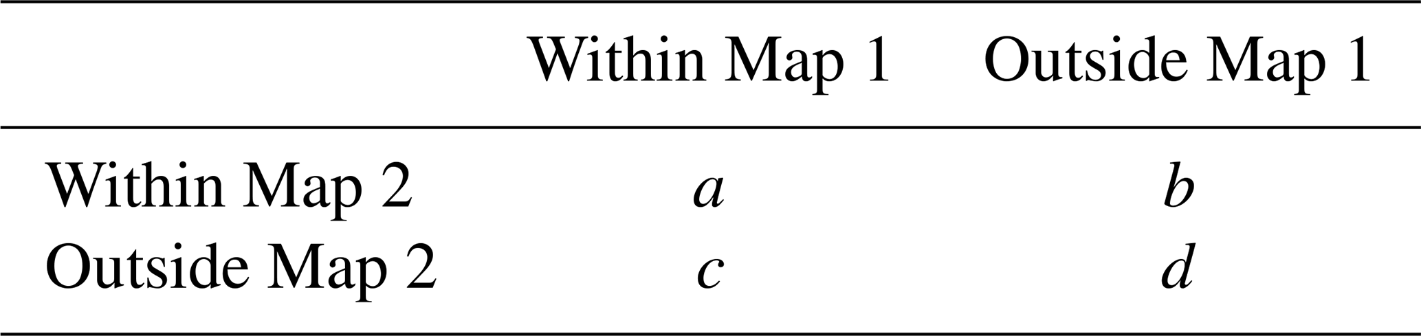
where a, b, and c denote the number of pixels within each river basin according to the contingency table in Table 1. Each combination of GFPLAIN, the JRC, and the GAR was evaluated with Eq. (2) for all 2776 river basins for the return periods 100 and 500 years separately: MAIGFPLAIN GAR-100, MAIGFPLAIN GAR-500, MAIGFPLAIN JRC-100, MAIGFPLAIN JRC-500, MAIGAR-100 JRC-100, and MAIGAR-500 JRC-500.
Table 1Contingency table for the pairwise model agreement evaluation as given by Eq. (2). The variables a, b, c, and d relate to the number of pixels within each river basin.
3.2.1 Spatial agreement clusters
We identified spatial clusters of basins with high and low model agreement relative to the mean, i.e. hot and cold spots, using the MAI-500 value for each river basin. This local spatial autocorrelation analysis was carried out in the software GeoDa, version 1.18 (Anselin et al., 2006). Positive spatial autocorrelation was found in high-agreement basins also having high-agreement neighbouring basins or low-agreement basins with low-agreement neighbours. More specifically, we used a local Moran statistic (Anselin, 1995), with 9999 random permutations, to identify significant clusters with pseudo p values >0.05. The significant clusters were mapped together with the original MAI-500 values to exhibit global patterns of the model agreement between the three flood models. The clusters are calculated irrespective of basin area since a majority of the basins are relatively consistent in size, and the agreement index in Eq. (1) ignores areas marked as dry.
3.2.2 Hydro-environmental attributes
The association between MAI-500 and several hydro-environmental attributes was then quantified for all 2776 river basins using statistic techniques in R (R Core Team, 2014). Basin level data for all attributes were retrieved from the datasets BasinATLAS version 1.0 (Linke et al., 2019) and HydroBASINS Level 5 (Lehner and Grill, 2013). Non-parametric measures were used for this evaluation since the response variable, MAI-500, did not fulfil the normality assumption of general linear models. An alpha level of 0.05 was used for all statistical tests.
The Kruskal–Wallis test by ranks (Hollander and Wolfe, 1973) was performed to control differences in MAI-500 values for the following factors: geographic region, river stream order (Lehner and Grill, 2013), and freshwater major habitat type (Abell et al., 2008). The freshwater major habitat types entail a combination of topographic, climatic, and hydrological properties since this classification is based on similarities in biological, chemical, and physical characteristics (WWF and TNC, 2019). All Kruskal–Wallis tests were supplemented with post hoc Wilcoxon rank-sum tests, performing pairwise comparisons between the groups. The Kruskal–Wallis tests used the Benjamini and Hochberg (1995) correction method for controlling false discovery rate. We also performed Kruskal–Wallis and Wilcoxon rank-sum tests to evaluate differences between the pairwise model agreement distributions (MAIGFPLAIN GAR-100, MAIGFPLAIN GAR-500, MAIGFPLAIN JRC-100, MAIGFPLAIN JRC-500, MAIGAR-100 JRC-100, and MAIGAR-500 JRC-500).
We then quantified the level of association between the model agreement and individual hydro-environmental attributes. Spearman's rank-order correlation coefficients (Harell and Dupont, 2021; Hollander and Wolfe, 1973; Spearman, 1904) were calculated for MAI-500, MAIGFPLAIN GAR-500, MAIGFPLAIN JRC-500, MAIGAR-500 JRC-500, and 23 control variables listed in Table 2. The resulting correlation coefficients between the model agreement scores and the hydro-environmental attributes were plotted in a correlogram (Wei and Simko, 2017).
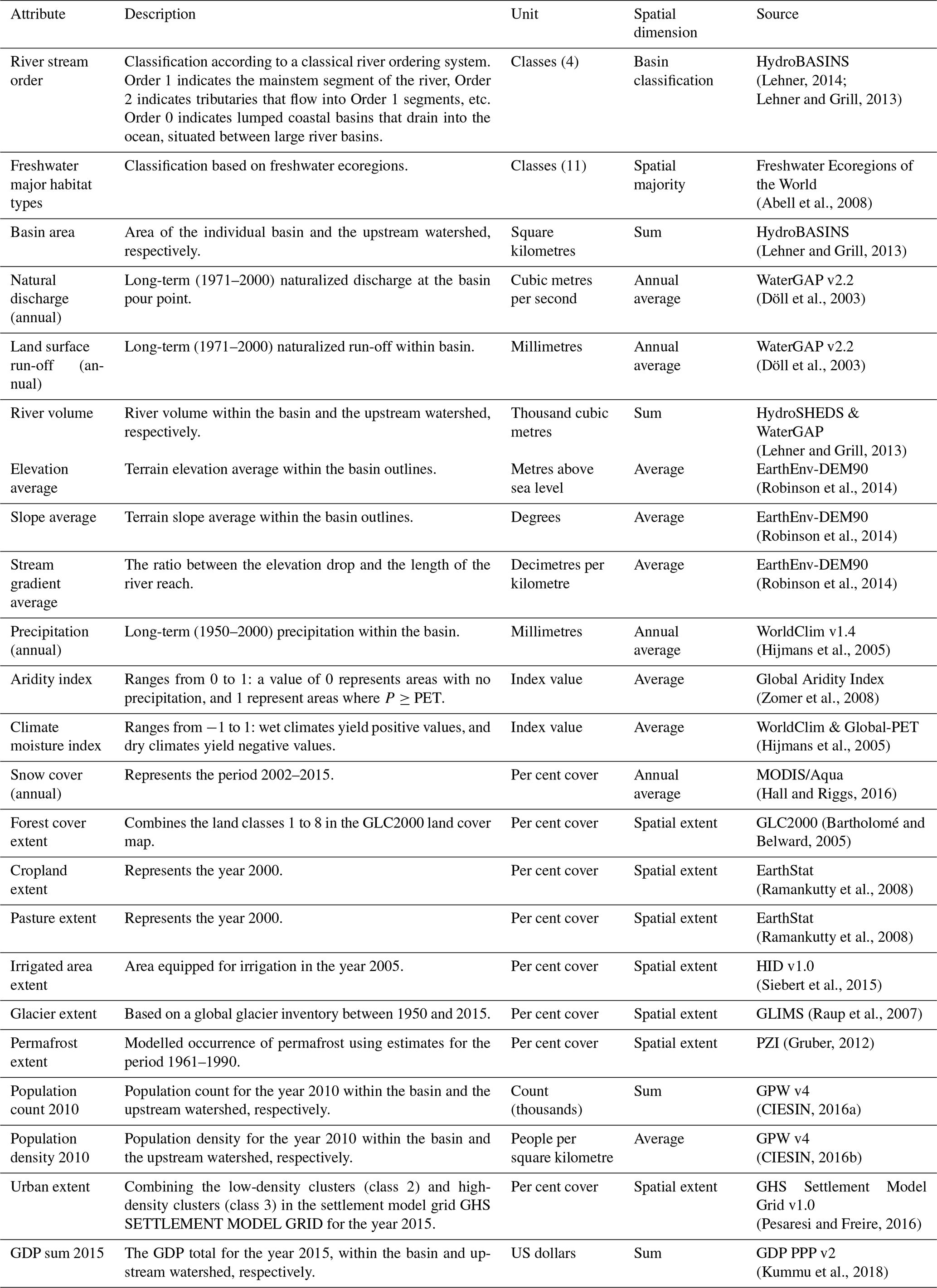
Table 2Control variables for which the association with the model agreement between the flood maps was evaluated. All control variables were retrieved from the dataset BasinATLAS version 1.0 (Linke et al., 2019), except river stream order and basin area, imported from the HydroBASINS dataset (Lehner and Grill, 2013). The upstream watershed is the total upstream watershed directly connected to the basin.
3.3 Country selection
The subsequent exposure and area analyses have been conducted for 26 countries in the global south: Bangladesh, Bolivia, Brazil, Cambodia, Central African Republic, Colombia, Republic of the Congo, Ecuador, Ghana, Guatemala, Honduras, India, Indonesia, Kenya, Lao People's Democratic Republic, Liberia, Malawi, Mozambique, Nicaragua, Nigeria, Peru, Sri Lanka, Thailand, Uganda, United Republic of Tanzania, and Viet Nam. These countries are situated in the eastern, middle, and western parts of Africa; South-East Asia; South Asia; Central America; and South America.
The countries were selected based on five criteria. First, we only included countries fully covered by all six datasets used for the comparative exposure analysis (GFPLAIN, JRC, GAR, GHS, HRSL, and WorldPop). Second, only countries belonging to the low-, lower-middle-, or upper middle-income groups were selected (Fig. 1), here classified using gross national income (GNI) per capita for the year 2015 (The World Bank, 2021b). The assumption was that, in general, the high-income countries have less need for global flood products since they tend to be more well equipped with national flood maps. Third, the selected countries all have a relatively high degree of riverine flood risk (Fig. 1), here represented by the combination of the population within the 100-year flood hazard map (intersecting the GHS and JRC) and actual disaster reports of people affected by riverine floods between 1900 and 2020 (Guha-Sapir et al., 2014). Fourth, we excluded countries with the main climate classification being arid or snowy according to the World Map of Köppen–Geiger (Beck et al., 2018). Finally, we have aimed to get a representative sample across the regions of the world.
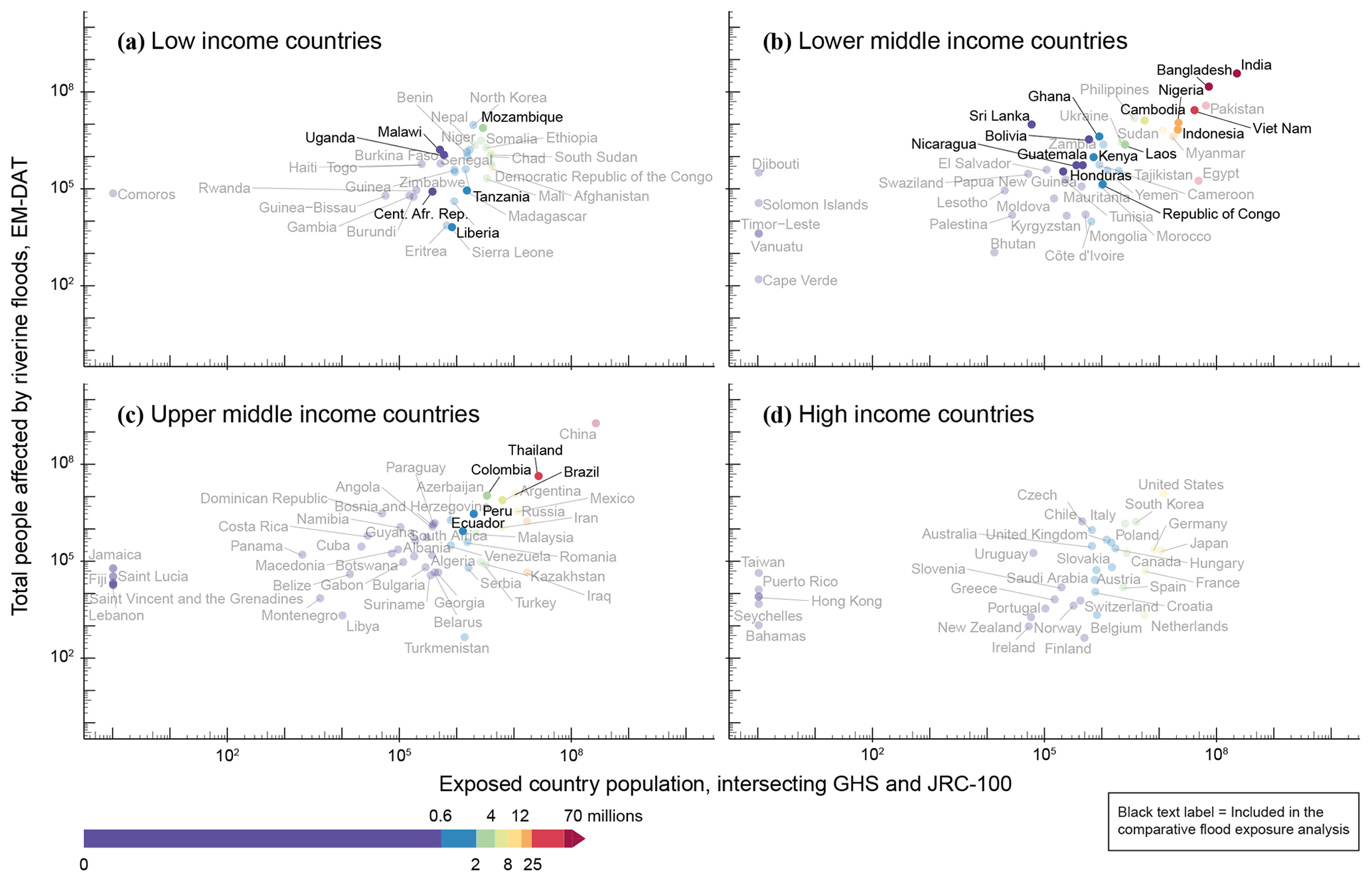
Figure 1Flood exposure in the 26 countries for which we conducted the comparative riverine flood exposure analysis, here marked with black text labels. Flood risk is represented here as the combination of the country population within the 100-year flood hazard map (intersecting the Global Human Settlement population grid count for 2015 with the JRC flood hazard map) and actual disaster reports of people affected by riverine floods between 1900 and 2020 as included in the Emergency Events Database EM-DAT. Please note that the axes have logarithmic scales. The country income classification is based on GNI per capita for the year 2015, given by the World Bank.
3.4 Exposure and area analysis
The number of people located in flood-prone zones was calculated for each country by intersecting the binary and masked images of GFPLAIN, JRC-500, JRC-100, GAR-500, and GAR-100 with the population maps of the GHS, the HRSL, and WorldPop. Country boundaries were outlined with the Global Administrative Unit Layers (GAUL) dataset for the year 2015 (FAO UN, 2015). The number of people living in flood-prone zones was then exported for all countries and dataset combinations. The population maps were also used for calculating country population totals, which have been compared to numbers provided by the World Bank in Table A7. The percentage of the country population living in flood-prone zones was then derived for each country and dataset combination.
For all area calculations of raster images, we used a pixel area function in Google Earth Engine (Gorelick et al., 2017) that minimizes projection distortions, which otherwise may be an issue when calculating areas over large regions. The function first calculated the area of each pixel using individual Lambert azimuthal equal-area projections for each block of pixels. The resulting grid of pixel areas was subsequently multiplied with the masked and binary images, for which the sum could be exported for each region of interest.
The total land surface area was calculated for all 26 countries by subtracting the total country area, as outlined by the polygons in the GAUL dataset (FAO UN, 2015), with the area of permanent surface water as given by the raster water mask MOD44W (Carroll et al., 2009). The area estimations of flood-prone zones, given by the binary and masked images of GFPLAIN, JRC-500, JRC-100, GAR-500, and GAR-100, were finally exported for all countries. The percentage of country area that is flood-prone was then derived for all countries and flood maps.
In this section, we first discuss the model agreement between the flood maps in Sect. 4.1 and then turn to the implications for riverine exposure analysis in Sect. 4.2.
4.1 Model agreement of flood-prone zones
4.1.1 Model agreement across model combinations
The overall spatial pattern of the floodplain map GFPLAIN resembles the flood hazard maps of the GAR more than the flood hazard maps of the JRC (Fig. 2). A possible explanation of this is that GFPLAIN and the GAR cover larger parts of each river network compared to the JRC since they exhibit lower inclusive thresholds for the upstream drainage area. Figure 2 shows that the model agreement between the floodplain map GFPLAIN and the flood hazard maps of the GAR is, on average, around 35 %. The corresponding agreement between GFPLAIN and the flood hazard maps of the JRC is around 30 %. These agreement levels are in line with the results of Trigg et al. (2016) when comparing the outputs of six global flood models for the African continent, finding an average model agreement of around 30 % to 40 %. It is also clear from Fig. 2 that there is a large spread of agreement scores across all 2776 river basins: all pairwise comparisons range between the maximum model agreement value of 100 % and very close to the minimum value of 0 %.
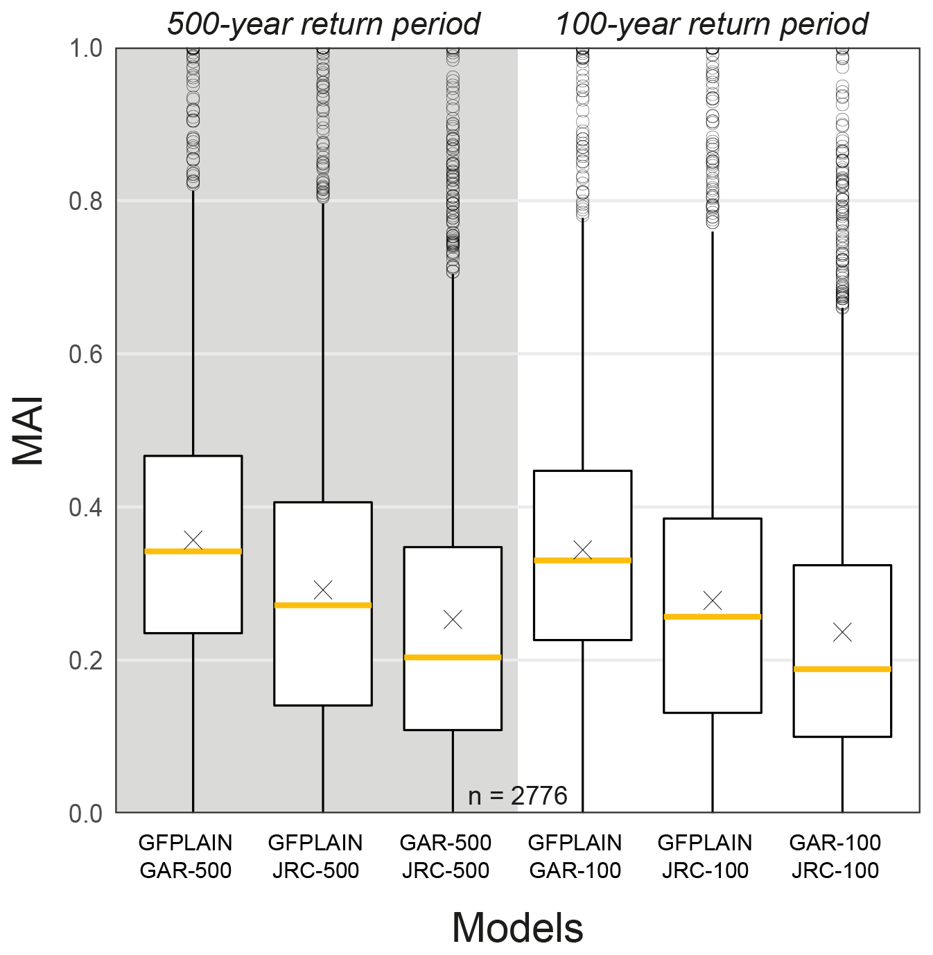
Figure 2Pairwise evaluation of model agreement between the hydrogeomorphic floodplain map GFPLAIN and the flood hazard maps the GAR and JRC, with a 100- and 500-year return period. The box hinges correspond to the first and third quartile, and the yellow line corresponds to the second quartile (median value). The mean value is indicated with a cross. The whiskers extend from the box hinges with maximum lengths equal to the inter-quartile range multiplied by a factor of 1.5. Values outside of the whiskers are indicated with dots. A higher return period shows higher agreement with GFPLAIN, but the choice of flood model influences the level of agreement even more. The flood hazard maps the GAR and JRC show the lowest level of agreement. The index has been calculated here for the 2776 river basins across the world that are covered by all three models.
The pairwise model agreement evaluation also confirms that the model agreement between GFPLAIN and the hazard maps is higher for the return period of 500 years compared to 100 years. This is consistent with previous findings in the literature about how the morphology of rivers, which the hydrogeomorphic floodplain maps delineate, is predominantly shaped by high-magnitude, low-recurrence flood events (Annis et al., 2019; Bhowmik, 1984; Nardi et al., 2018). Figure 2 pinpoints, however, that choice of hazard model has a greater influence on the degree of model agreement with GFPLAIN compared to the choice of return period.
Contrary to expectations, the model agreement between the hazard maps of the JRC and GAR is lower compared to their agreement with GFPLAIN. The median agreement values across all river basins are found to be 0.34 for GFPLAIN and GAR-500, 0.27 for GFPLAIN and JRC-500, and 0.20 for GAR-500 and JRC-500. The reasons for this result are not evident, but it supports earlier findings of significant disagreement among individual global flood models (Trigg et al., 2016; Ward et al., 2015). All distributions from the pairwise model agreement evaluation show positive skewness, meaning that the bulk of river basins have low values (Fig. 2). The portion of river basins having low agreement scores is highest for the GAR and JRC comparison, illustrated by the relatively big differences between the average and median values. A Kruskal–Wallis test showed that there is a significant difference in model agreement between the distributions (H(5)=1217, p<0.001); the pairwise comparisons from the post hoc test can be found in Table A3.
4.1.2 Model agreement across geographic conditions
We also analysed how MAI-500, the model agreement between GFPLAIN, GAR-500, and JRC-500, varies across space and a set of hydro-environmental groups. We chose to represent the model agreement with MAI-500 since we generally found a higher model agreement using the 500-year return period compared to the 100-year return period. Figure 3 provides the spatial distribution of MAI-500 across all 2776 river basins and local clusters of high and low model agreement relative to the mean, as identified from the spatial autocorrelation analysis. These maps suggest that the model agreement is associated with factors related to climate, topography, and coastal proximity.
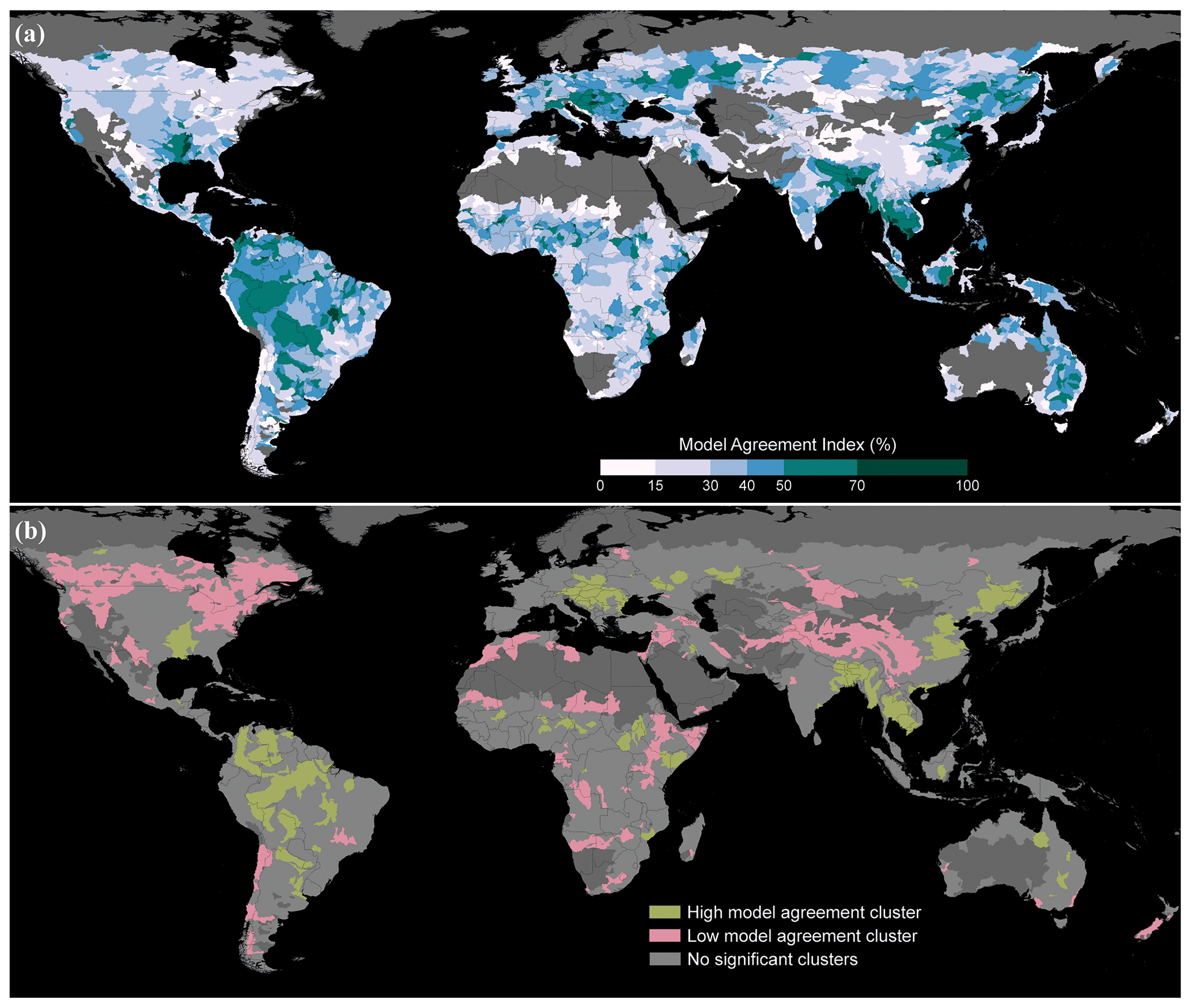
Figure 3(a) Spatial distribution of MAI-500, the model agreement between the hydrogeomorphic floodplain map GFPLAIN and the flood hazard maps the GAR and JRC with a 500-year return period. The model agreement index ranges between 0 % (no agreement) and 100 % (full agreement) and was calculated here for all the river basins of the world that are covered by all three models. (b) Local clusters of river basins with high or low agreement values relative to the mean, identified from the spatial autocorrelation analysis.
The river basins with the highest model agreement are generally located in humid regions (Fig. 3). For instance, it is the equatorial humid climate regions that exhibit the highest model agreement in the South American continent, including the north-western part of Brazil and the north-eastern part of Peru. The high-agreement cluster in North America, near the Mississippi River Delta, and the high-agreement cluster in south-eastern Europe are also situated in warm temperate and fully humid regions. In contrast, a poor model agreement is generally found in dry regions. The regions in North America with cold climate entail large clusters of basins with a low model agreement. Arid desert regions also exhibit low model agreement clusters, such as the Kalahari Desert in southern Africa.
Relating to topography, Fig. 3 also shows that alpine regions like the Andes in South America and high-mountain Asia exhibit poor model agreement. This can, at least partly, be explained by the same regions being dry. It also seems possible that very steep regions would be prone to error. However, very flat regions also tend to exhibit poor model agreement across climate types. This may be exemplified by the flat grassland of the humid Pampa region in Argentina and the flat inland areas on the tropical islands of Indonesia.
Figure 3a furthermore illustrates that coastal river basins seem to exhibit low model agreement, visible as white lines along many coastlines. This tendency is not captured well by the clusters in Fig. 3b since one single low-agreement basin near the coast would not count as a cluster. A possible explanation for the low agreement in coastal river basins might be due to complex flood hydraulics yielding different results, in line with previous findings of low agreement in deltas (Dottori et al., 2016a; Trigg et al., 2016). For instance, GFPLAIN tends to miss floodplain areas near the coast (on the order of a few kilometres), possibly because these areas are challenging to detect with hydrogeomorphic analysis. The individual riverine flood maps might also differ in their respective demarcation to coastal flooding. Another possible explanation for the low model agreement in coastal river basins is that the JRC might miss small coastal watersheds compared to GAR and GFPLAIN due to having a higher threshold of upstream drainage area. It can also be seen in Fig. 3 that major river deltas often exhibit high model agreement on the basin level, as exemplified by the Mississippi River Delta in the US and the Mekong River Delta in Viet Nam and Cambodia. This is an indication that the volume of the river also affects the model agreement, which seems possible since large river discharge imposes large forces on the surrounding landforms, the very shapes that GFPLAIN aims to capture.
Thus far, we have elaborated on what might cause the spatial variation in MAI-500 based on a visual inspection of the global maps in Fig. 3. We also quantified these results by assessing how the MAI-500 value varies between a set of factoring groups: geographic region, river stream order, and freshwater major habitat type. Across the basins situated in each geographic region, Fig. 4a conveys that the highest model agreement can, on average, be found in South America (39 %) and Central and South-East Asia (39 %), while North America (29 %) and Africa (32 %) exhibit the lowest model agreement. This supports, again, that humid regions tend to perform better compared to dry regions. The Kruskal–Wallis test showed that there is a significant difference in model agreement between the regions (H(6)=146, p<0.001); the pairwise comparisons from the post hoc test can be found in Table A4.
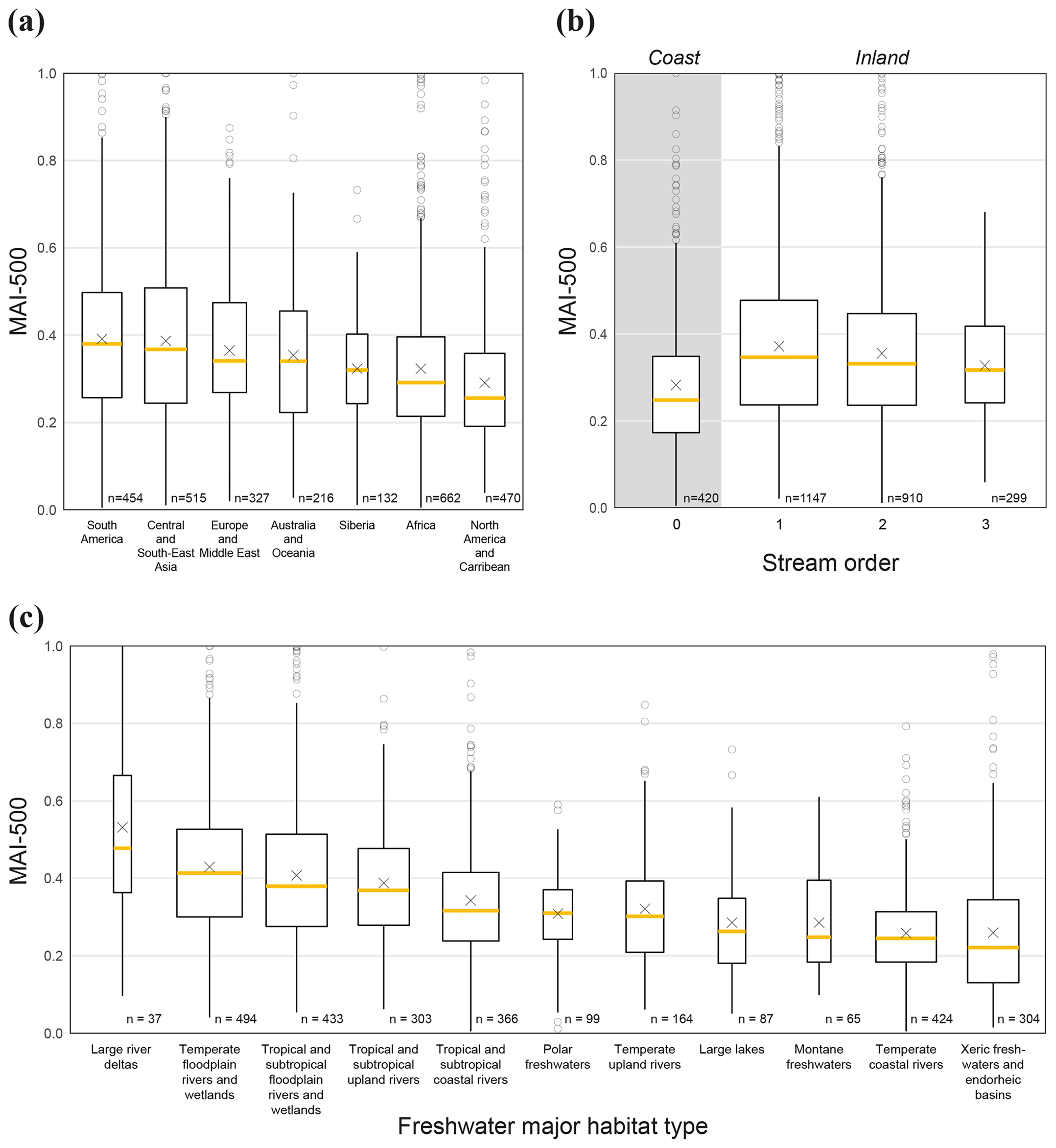
Figure 4How the model agreement between GFPLAIN, GAR-500, and JRC-500 varies with (a) geographic region, (b) river stream order, and (c) freshwater major habitat type. The model agreement index ranges between 0 % (no agreement) and 100 % (full agreement) and was calculated here for all the river basins of the world that are covered by all three models. The box hinges correspond to the first and third quartile, and the yellow line corresponds to the second quartile (median value). The mean value is indicated with a cross. The whiskers extend from the box hinges with maximum lengths equal to the inter-quartile range multiplied by a factor of 1.5. Values outside of the whiskers are indicated with dots. The number of river basins corresponding to each group is indicated in numbers and box width. Coastal river basins tend to have lower model agreement scores compared to inland river basins. The freshwater major habitat type specifies the spatially dominating habitat type in each river basin (WWF and TNC, 2019). The habitat type “large river deltas” only includes regions that exhibit both deltaic physical features and deltaic fauna. The habitat type “large lakes” includes river basins that are dominated by large lentic systems. The grouping of basins into geographic regions follows the HydroBASINS dataset.
Figure 4b illustrates how MAI-500 varies with river stream order, supporting that model agreement tends to be negatively associated with coastal proximity. Furthermore, the Kruskal–Wallis test showed that the model agreement significantly varies between river stream orders (H(3)=101, p<0.001). More specifically, the model agreement in coastal basins, stream order 0, was identified as significantly lower compared to inland stream order groups, verified by the post hoc Wilcoxon rank test (p values <0.001; see Table A5).
We now move on to the freshwater major habitat types, a classification based on the spatially dominating habitat type in each river basin (WWF and TNC, 2019). Before presenting the model agreement variations between the habitat types, however, we point out that a classification on the river basin level will inevitably contain multiple smaller habitat types. For instance, the habitat type “large lakes” includes river basins that are dominated by large lentic systems, in our case covering three large regions: Lake Baikal in Siberia, Lake Malawi in Africa, and Michigan–Huron in North America. But a river basin of this habitat type can, for example, also contain grassy savannas or swamps (WWF and TNC, 2019). Another point is that the habitat type “large river deltas” only includes regions that exhibit both deltaic physical features and deltaic fauna (WWF and TNC, 2019). This habitat type covers four large regions within our analysed river basins: the Niger Delta in Nigeria, the Mekong Delta in Viet Nam and Cambodia, the Orinoco Delta in Venezuela, and Brazilian delta regions between the rivers Amazon and Mearim. In other words, deltas without the characteristic deltaic fauna do not belong to this habitat type. For instance, the river basins containing the Mississippi River Delta belong to the habitat type “temperate floodplain rivers and wetland complexes”. Another point is that the difference between rivers classified as floodplain rivers and upland rivers is the presence of cyclically flooded floodplains. Floodplain rivers are characterized by having cyclically flooded floodplains (today or historically), while the upland rivers are not (WWF and TNC, 2019). Upland rivers can for instance be tributaries of large river systems.
Figure 4c shows how the model agreement varies between the freshwater major habitat types. Floodplain rivers, in temperate and tropical climate regions, exhibit higher model agreement compared to upland rivers, followed by coastal rivers. We can also see, as previously discussed, that freshwaters in arid, here expressed as xeric, and montane regions exhibit poor model agreement. The group “large river deltas” is ranked as having the highest model agreement, clearly influenced by the high agreement in large river deltas, like the Mekong. These results should be interpreted with caution, however, due to the unbalanced sample sizes between the groups (Fig. 4c). Nonetheless, the inherent order between the groups supports previous discussion about how factors related to climate, topography, coastal proximity, and river volume affect MAI-500 values. The Kruskal–Wallis test showed that the agreement difference is significant between the habitat types (H(10)=478, p<0.001). The pairwise comparisons from the post hoc test can be found in Table A6.
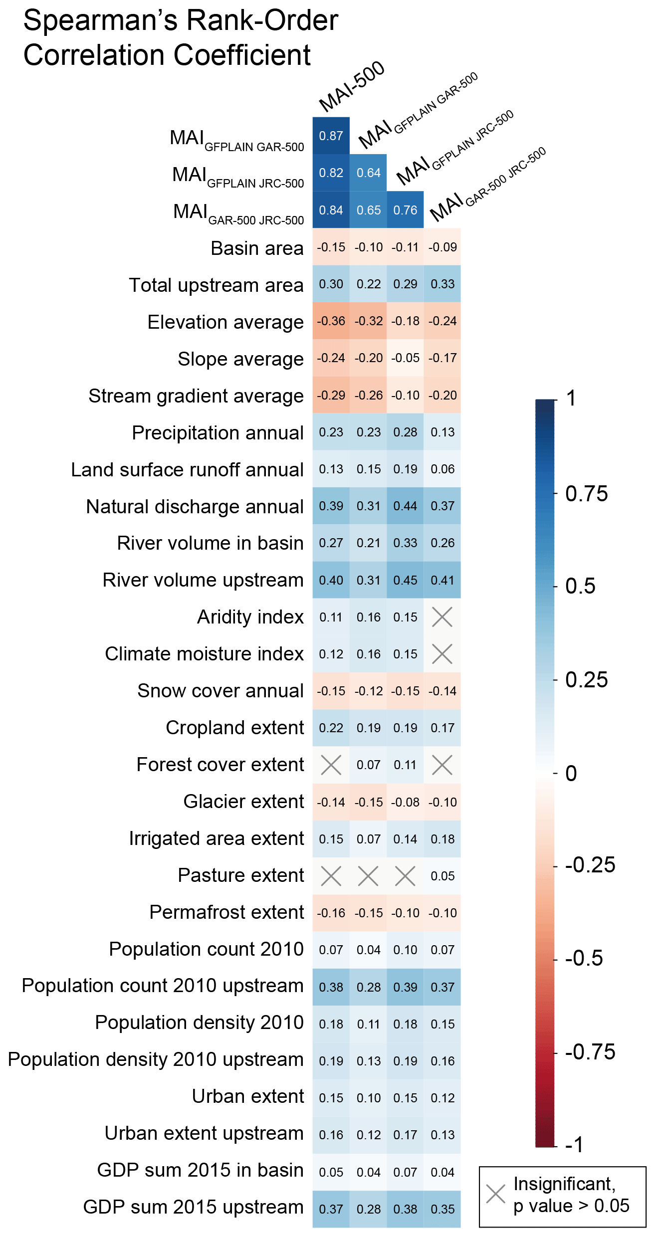
Figure 5Spearman's rank-order correlation coefficients between the flood model agreement scores and 27 hydro-environmental attributes. Wetter conditions due to climate (precipitation, land surface run-off) and river size (e.g. river volume, natural discharge) are positively associated with the model agreement between the flood maps. Topographic variables like high altitude (elevation) and steep slope (e.g. slope and stream gradient) are negatively associated with the model agreement, especially between GFPLAIN and GAR-500. Please note that the aridity index increases with humidity.
4.1.3 Model agreement association with hydro-environmental attributes
Section 4.1 has so far demonstrated that MAI-500, the level of model agreement between GFPLAIN, GAR-500, and JRC-500, is linked to factors related to climate, topography, coastal proximity, and river volume. We have done this by visually exploring the spatial pattern of the model agreement and by grouping the values according to geographic region, river stream order, and freshwater major habitat type. Each of these habitat groups contains a variety of geographic characteristics, so we also analysed the level of association between model agreement and individual hydro-environmental attributes and investigated whether the association differs between the model agreement pairs.
Figure 5 presents the Spearman rank-order correlation coefficients in a correlogram, supporting the statement that wet regions tend to exhibit higher model agreement compared to dry regions. Precipitation, land surface run-off, the aridity index, and the climate moisture index are positively associated with the level of model agreement. Precipitation exhibits the strongest positive association among these variables, especially for MAIGFPLAIN JRC-500. The association levels between MAIGAR-500 JRC-500 and these climatic variables are, however, relatively weak or even insignificant (the aridity index and the climate moisture index). In other words, the level of agreement between GFPLAIN and the hazard maps seems to be positively influenced by a wet climate, while the agreement between the JRC and GAR seems to be controlled by other factors. This result further supports the comment that the skill of hydrogeomorphic floodplain maps to represent flood hazard depends on the availability of water.
The variables that represent the magnitude of river discharge also exhibit a positive association with the model agreement in an even stronger sense compared to the previously mentioned climatic variables (Fig. 5). This is particularly evident for the variables natural discharge and upstream river volume, having moderate to strong positive association with all model agreement distributions. For the very same reason, we can see that the size of the upstream drainage area exhibits a positive association with the model agreement but to a moderate degree. As previously discussed, increased discharge means larger forces forming the landscape and hence more well-defined floodplains. The size of the river basin being evaluated, on the other hand, co-variates with the model agreement in a weak negative direction. One explanation for this is that very small river basins get maximum model agreement scores when they are fully covered by all three flood models.
The association between model agreement and the variables elevation, slope, and stream gradient is significant in a negative direction (Fig. 5). This finding supports previous discussion about how high-altitude and steep regions tend to exhibit poor model agreement. The association between these topographic variables is strongest for the model agreement between GFPLAIN and the GAR, whereas the association is weakest for the agreement between GFPLAIN and the JRC. The reason for this result is not evident, but one explanation could be that the one-dimensional hydraulic modelling of the GAR tends to be sensitive to these topographic variations. These findings may also be somewhat limited since the relationship between model agreement and, for instance, the slope is not monotonic: we have already observed how many very flat areas also exhibit poor model agreement (Fig. 3).
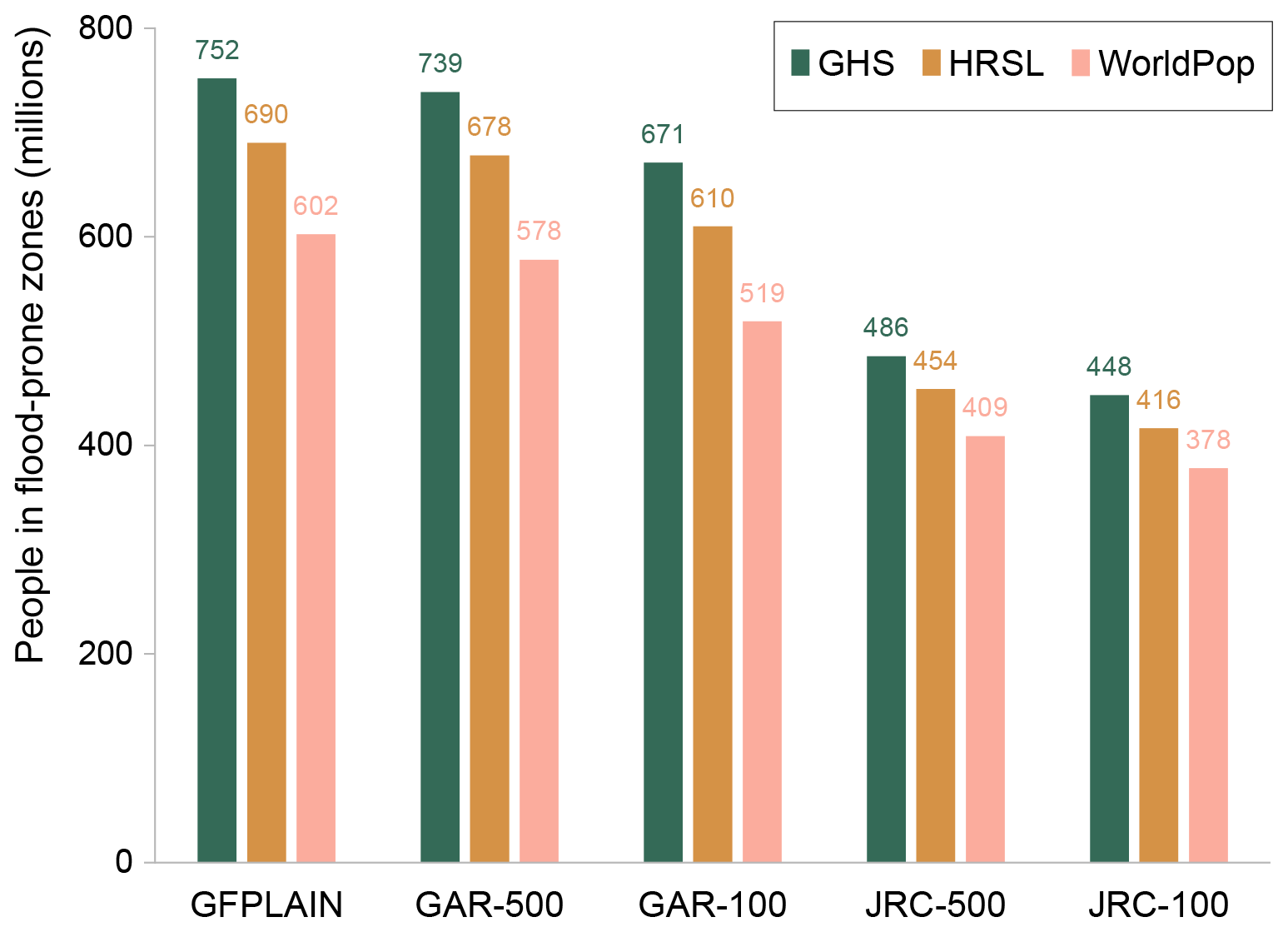
Figure 6Total exposed population (millions) across all 26 countries, comparing the hydrogeomorphic floodplain map GFPLAIN with the flood hazard maps the GAR and JRC with 100- and 500-year return periods. The population estimates are given by the Global Human Settlement population grid, the High Resolution Settlement Layer, and WorldPop. The floodplain map GFPLAIN yields the highest exposure estimates even though GAR-500 covers a slightly larger total area. The choice of flood and population maps affects the results more than the choice of the return period.
The overall association between model agreement and the anthropogenic influences (population count, GDP) and the land cover characteristics (e.g. urban extent, cropland extent) is weak. These results are likely to be related to the scale of the analysis; any possible association would be averaged out on the aggregated basin level. Nardi et al. (2018) predominantly found consistencies between a hydrogeomorphic floodplain map and flood hazard maps in areas unaltered by humans. However, the population count and GDP in the upstream watershed regions show moderate positive association with the model agreement scores since these variables are also correlated with the variables that represent the magnitude of river discharge (upstream drainage area, upstream river volume, and natural discharge).
4.2 Implications for exposure analysis
Our analysis has shown that the level of agreement between GFPLAIN and the GAR and JRC flood hazard maps is, on average, higher compared to the agreement between the GAR and JRC. Furthermore, we have shown that the model agreement is linked to factors related to climate, topography, river size, and coastal proximity. We further analysed how these differences affect riverine flood exposure analysis, which we have conducted for 26 countries using the GHS, WorldPop, and HRSL population maps.
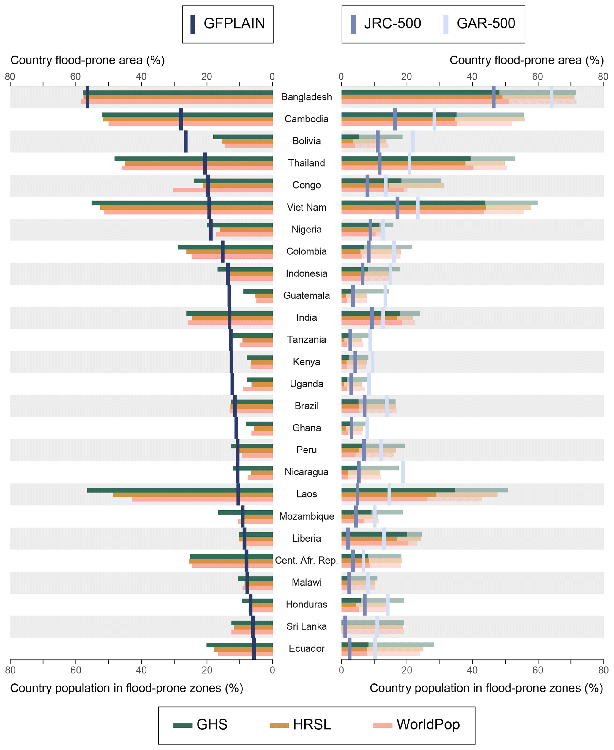
Figure 7Riverine flood exposure estimates, aggregated at country level, using the hydrogeomorphic floodplain map GFPLAIN (bars on the left) and the flood hazard maps of the JRC (bars on the right) and GAR (shaded bars on the right) with a 500-year return period. The green, orange, and pink horizontal bars indicate the percentage of the country's population in flood-prone zones using the population maps Global Human Settlement population grid, High Resolution Settlement Layer, and WorldPop, respectively. The vertical blue bars indicate the percentage of land area that is flood-prone. Country boundaries follow the GAUL 2015 dataset, and permanent water has been masked by the product MOD44W.
The flood hazard maps GAR-500 and GAR-100 cover an area of and km2 across the 26 countries, while the floodplain map GFPLAIN covers km2. The hazard maps JRC-500 and JRC-100 cover an area of and km2, respectively. One explanation for this large difference is that the GAR and GFPLAIN include smaller rivers compared to the JRC. Figure 6 shows the flood exposure estimates of each map combination, aggregated across all 26 countries. Interestingly, GFPLAIN yields a larger exposure estimate compared to the GAR and JRC, even though GAR-500 covers a larger total area than GFPLAIN. One explanation of the higher population estimate given by GFPLAIN is that the floodplain map covers a larger area of densely populated regions in India, resulting in 44 million more exposed people with GFPLAIN compared to GAR-500 (using the HRSL population map). This difference is, however, counteracted by the instances where GAR-500 yields larger exposure estimates, for example, 21 million more exposed people in Bangladesh.
We would like to highlight that (1) the choice of flood model influences the exposure estimates to a higher degree than the choice of the hazard return period. We think that this finding provides an important perspective to end users of global flood maps; (2) we observe an inherent order across the population maps (), which can be explained by the varying population totals across these datasets (Table A7). WorldPop, for instance, exhibits considerably lower population values for all 26 countries. Scaling the country totals would enable a more consistent comparison of the exposure hit between the individual population datasets. We did not scale the population estimates, however, since this study aims to capture how dataset choice affects exposure estimates.
Let us now turn to discuss how the riverine exposure estimates vary across individual countries and map combinations. Figure 7 presents the flood-prone area and exposed population as proportions for each country. Among our analysed 26 countries, countries in South Asia and South-East Asia stand out as having the highest riverine flood exposure. For instance, the largest number of people living within riverine flood-prone zones can be found in India (346 million), Bangladesh (100 million), Viet Nam (53 million), and Indonesia (37 million). The proportion of exposed people is largest for Bangladesh (59 %), Viet Nam (54 %), Cambodia (53 %), and Laos (50 %). The proportion of land area that is flood-prone is largest for Bangladesh (57 %), Cambodia (28 %), Bolivia (26 %), and Thailand (21 %). The numbers listed here represent the intersection of GFPLAIN and the HRSL. All results of the area calculations and exposure estimations have been made available in Tables A8–A10.
It can also be seen in Fig. 7 that GAR-500 covers the largest area in 17 countries, whereas GFPLAIN covers the largest area in the remaining 9 countries. Honduras is the only country where the JRC covers a larger area compared to GFPLAIN. This is explained by the fact that coastal areas make up a large part of this country, and these are more often masked from GFPLAIN compared to the JRC. This tendency is not consistent, however, and for instance does not apply to Sri Lanka. One of the issues emerging from this finding is that masked areas near the coast can affect the exposure analysis result. Even though one would not expect the usage of riverine flood maps for estimating coastal flood risk, it might still affect riverine exposure estimations on, say, the country level since the coastal areas also tend to be densely populated. This is most certainly the case in Liberia. GFPLAIN covers a larger area compared to the JRC but misses parts of the densely populated coastal city Monrovia, resulting in an exposure estimate that is smaller by 0.43 million compared to the JRC. At the same time, variations among the flood maps can also affect the coverage of inland cities, as in the case of Colombia. GAR-500 covers a larger area compared to GFPLAIN, but GFPLAIN yields an exposure estimate that is larger by 4.5 million from covering a larger part of the capital city Bogotá.
As far as the influence of the return period is concerned, the difference between the exposure estimates of JRC-500 and JRC-100 is largely proportional to the corresponding area difference. This is also the case for the hazard maps of the GAR, with some exceptions. The area ratio between GAR-500 and GAR-100 in Thailand, for example, is 1.09, while the corresponding exposure ratio using the HRSL is 1.83. Similar results can be found for Indonesia (1.04 compared to 1.22), Brazil (1.03 compared to 1.17), and Colombia (1.02 compared to 1.13). This finding might reveal how populations in these countries tend to live outside but close to the 100-year flood hazard zone.
Figure 8 illustrates some of the implications that the dataset differences have for riverine exposure analysis. Figure 8a covers a part of the Amazon River in Brazil and, in Sect. 4.1.2, is identified as a high-model-agreement cluster. The spatial patterns of GFPLAIN, JRC-500, and GAR-500 are quite similar for this major river. GFPLAIN and the GAR cover smaller river tributaries compared to the JRC, but this difference does not affect the exposure estimates since the population is clustered in the city of Manaus near the main river. Figure 8b illustrates a major discrepancy in the handling of coastal regions between the individual models, exemplified by the Niger Delta in Nigeria. The JRC covers the entire river basin, while both GFPLAIN and the GAR have masked the coastal areas to different degrees. These discrepancies affect the exposure hits in cities like Port Harcourt and Warri.
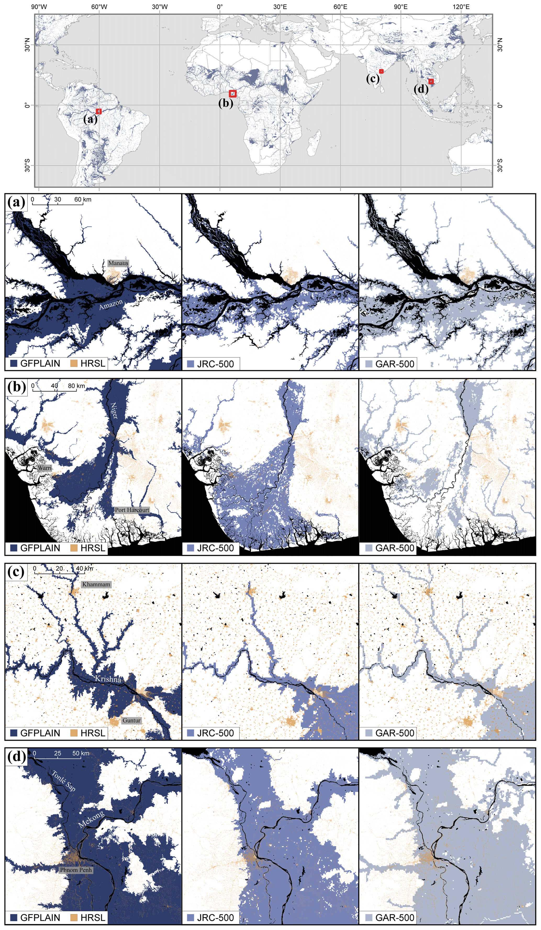
Figure 8Spatial patterns of the hydrogeomorphic floodplain map GFPLAIN compared to the JRC and GAR flood hazard maps with a 500-year return period for the rivers (a) Amazon in Brazil, (b) Niger in Nigeria, (c) Krishna in India, and (d) the Mekong in Cambodia. The brown pixels indicate settlements mapped with the High Resolution Settlement Layer. The black pixels indicate the permanent water mask.
Figure 8c covers a part of the Krishna River in India. This map also illustrates how GFPLAIN and the GAR include smaller rivers than the JRC, as is the case for the river tributaries north of the city Khammam. We can also see how GFPLAIN covers a smaller area in the south-eastern map corner but reaches the city of Guntur, nonetheless, in contrast to the GAR and JRC. Figure 8d covers a part of the Mekong River in Cambodia, also identified as a high-model-agreement cluster in Sect. 4.1.2. The spatial pattern is indeed quite similar between the flood maps for this large river but with some discrepancy. For instance, GFPLAIN does not exhibit the same gaps in the flood extent, as can be seen in the northern part of the JRC and GAR flood maps. These gaps represent hilly areas that in reality would be unlikely to flood and could be an artefact of the hydrogeomorphic delineation method. GFPLAIN furthermore covers a larger portion of the capital Phnom Penh, affecting the exposure hits.
In closing this section, we want to pinpoint one last remark from the findings illustrated by Fig. 7 related to the inherent order between the population maps (). As discussed, a scaling of the country totals would enable a more consistent comparison of the exposure hit between the individual population datasets. Nonetheless, we have indeed conducted a form of scaling in Fig. 7 when normalizing the exposed population estimates with the population totals. The proportion of the exposed population is still generally highest for the GHS population map, whereas the results vary for the HRSL and WorldPop. This can be contrasted to the study of Smith et al. (2019), finding considerably lower exposure estimates for the HRSL compared to the GHS and WorldPop when scaling the demographic datasets to share the country totals. But an important aspect of their finding, besides the scaling of country totals, is that the hazard data need to be high-resolution to make use of the detailed settlement representation of the HRSL (Smith et al., 2019). We think that this also highlights an important aspect of the usability of hydrogeomorphic floodplain maps in riverine exposure analysis. The opportunity to delineate high-resolution floodplain maps from new terrain models can play an important role in conducting riverine flood exposure estimations in data-poor regions if one wishes to make the best use of the detailed representations of new population maps, like the HRSL.
In this paper, we evaluated model agreement between the hydrogeomorphic floodplain map GFPLAIN with the flood hazard maps of the JRC and GAR across geographic conditions and a set of hydro-environmental attributes. We demonstrated that the level of model agreement between GFPLAIN and the flood hazard maps is linked to climatic conditions, topography, coastal proximity, and river volume. We also conducted riverine exposure analysis for 26 countries by intersecting the flood maps with three demographic datasets to explore how model differences affect riverine flood exposure estimations. Our findings can be summarized by three main points.
First, our results confirm that the consistency between GFPLAIN and the flood hazard maps increases with the return period. The choice of model for the flood hazard map is, nevertheless, more important for evaluating model agreement on the river basin level and, also, for affecting the results of exposure analysis.
Second, our study confirms that the results of riverine exposure analysis are highly dependent upon the choice of datasets. Contrary to expectations, the model agreement between the JRC and GAR hazard maps is lower compared to their agreement with GFPLAIN. The median agreement values across all river basins are found to be 0.34 for GFPLAIN and GAR-500, 0.27 for GFPLAIN and JRC-500, and 0.20 for GAR-500 and JRC-500. There is a large spread across all basins, however, ranging between the maximum model agreement value 1 and very close to the minimum value 0. This finding (yet again) stresses the uncertainties in global flood models, suggesting that users might benefit by using an ensemble of models as a way of precaution.
Third, the agreement level between GFPLAIN and the flood hazard maps suggests that hydrogeomorphic terrain analysis can indeed be viewed as a valuable way of estimating flood-prone zones, especially in data-poor regions. The highest model agreement was generally found for large rivers in temperate or tropical climate regions. However, we do not wish to reduce hydrogeomorphic methods as mere substitutes for global flood models: the individual methodologies ultimately serve different purposes. Furthermore, floodplain maps built by hydrogeomorphic terrain analysis should be used with caution in regions that are dry, steep, very flat, or near the coast. The tendency by GFPLAIN to not cover coastal areas may in many cases affect the riverine flood exposure estimates, even on the country level, since coastal areas also tend to be densely populated.
Inter-model comparisons like this study do not answer the question of how well the individual flood layers agree with actual flood events. Future research can build upon this comparative study by conducting a validation analysis using flood delineation from satellite imagery, similar to the work by Bernhofen et al. (2018) or Hawker et al. (2020) but for a larger set of regions across the world (e.g. using the recent Global Flood Database; Tellman et al., 2021). Future studies can also investigate how model agreement varies with the fluvial geomorphology of the rivers (e.g. as given by the global river classification dataset GloRiC; Ouellet Dallaire et al., 2019) or land cover (e.g. as given by the ESA CCI 2015 land cover map; ESA, 2017).
To conclude, this study provided initial insights on how and where hydrogeomorphic floodplain maps could serve as candidates for identifying flood-prone areas in riverine flood risk studies. One particular benefit of hydrogeomorphic terrain analysis is that it does not require hydrological information to produce high-resolution floodplain maps whenever refined terrain models become available, also enabling the mapping of finer parts of the river network. This could particularly play an important role in riverine flood exposure analysis as the detail of the hazard layer needs to meet the detail of the settlement layer to avoid overestimations of flood exposure, which is especially important in dispersed rural regions.
Table A1A technical summary of the datasets used for riverine flood exposure analysis.
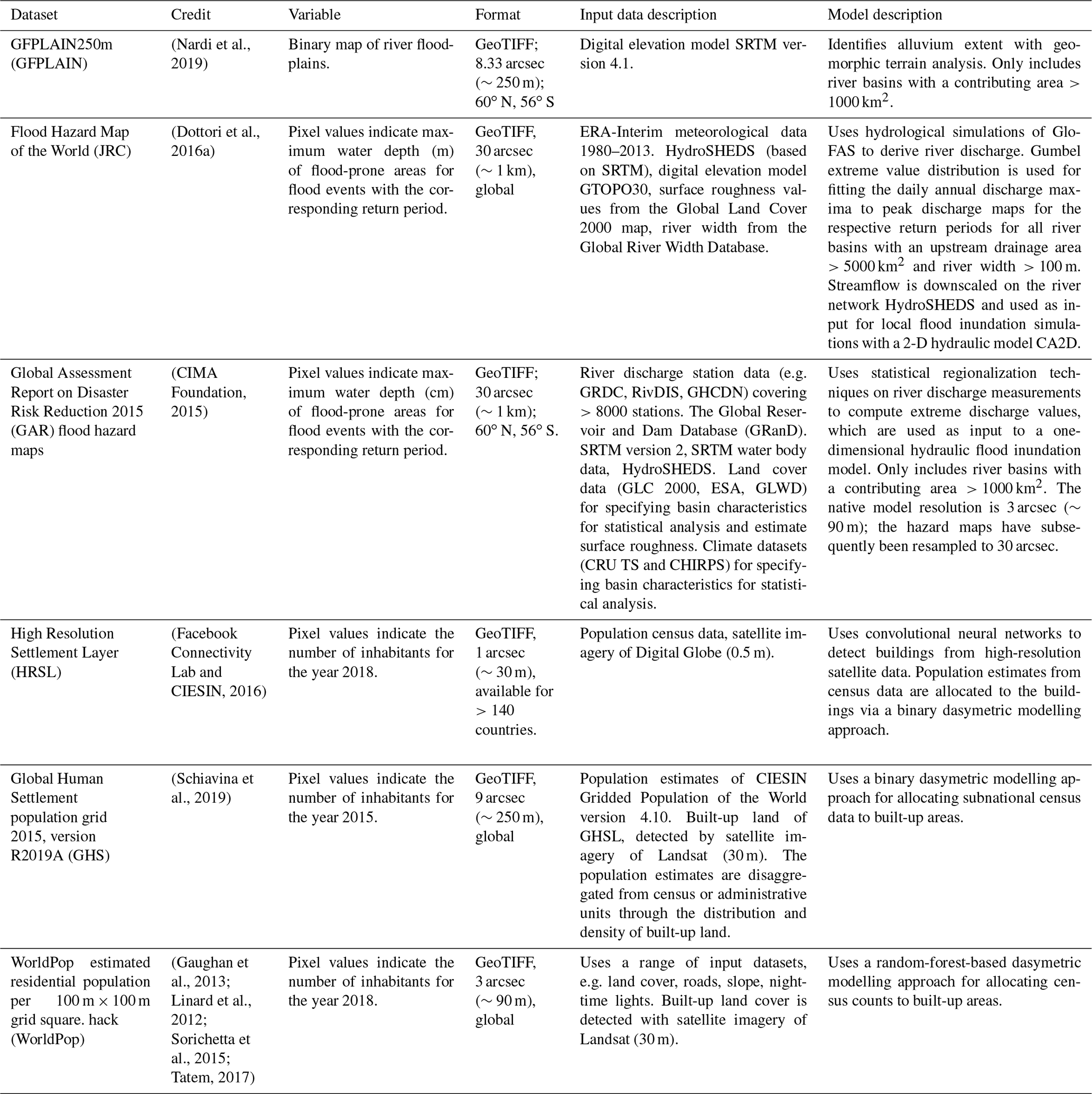
Table A2Descriptive statistics, expressed in square kilometres, of the 2776 river basins included in the analysis.
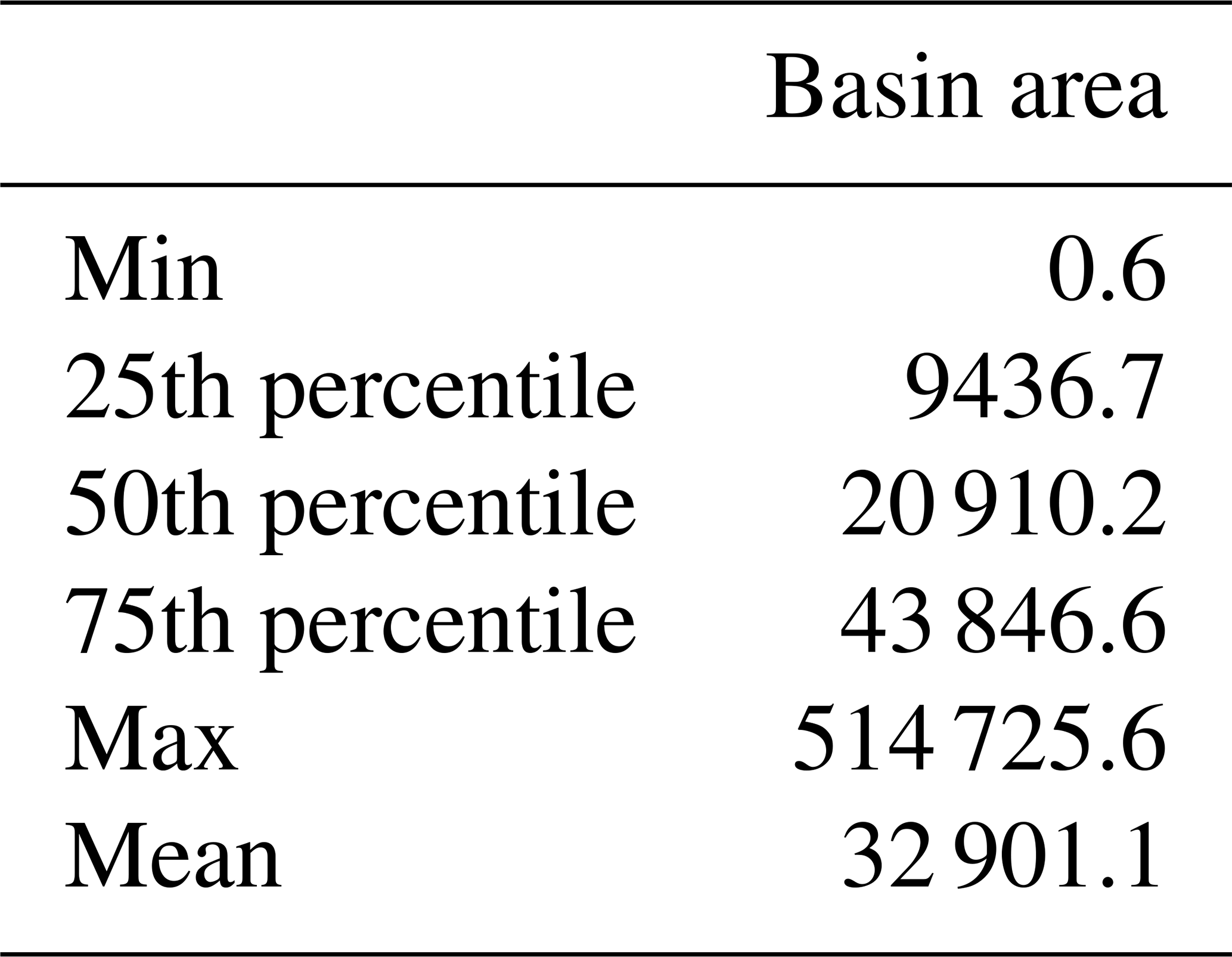
Table A3Summary statistics and pairwise comparisons of the model agreement between each pair of flood maps. A Kruskal–Wallis test showed that there is a significant difference in model agreement between groups (H(5)=1217, p<0.001). The pairwise comparisons, for detecting significant differences between the groups, have been conducted using the Wilcoxon rank-sum test with continuity correction.
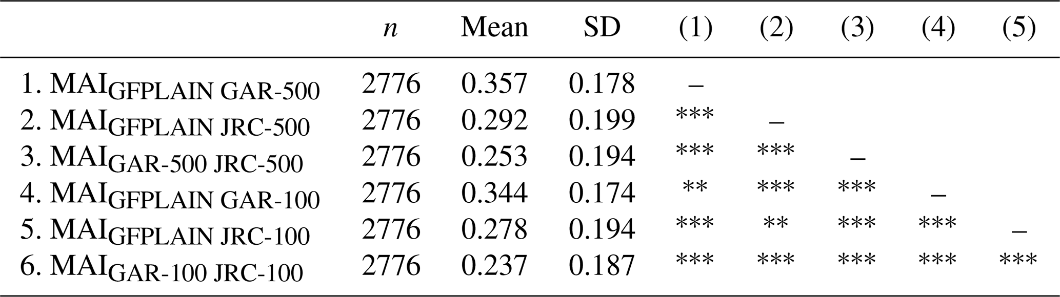
Note: ∗ p<0.05, p<0.01, p<0.001.
Table A4Summary statistics and pairwise comparisons of how MAI-500 (the model agreement index of GFPLAIN, GAR-500, and JRC-500) varies with different geographic regions. A Kruskal–Wallis test showed that there is a significant difference in model agreement between the regions (H(6)=146, p<0.001). The pairwise comparisons, for detecting significant differences between the regions, have been conducted using the Wilcoxon rank-sum test with continuity correction.
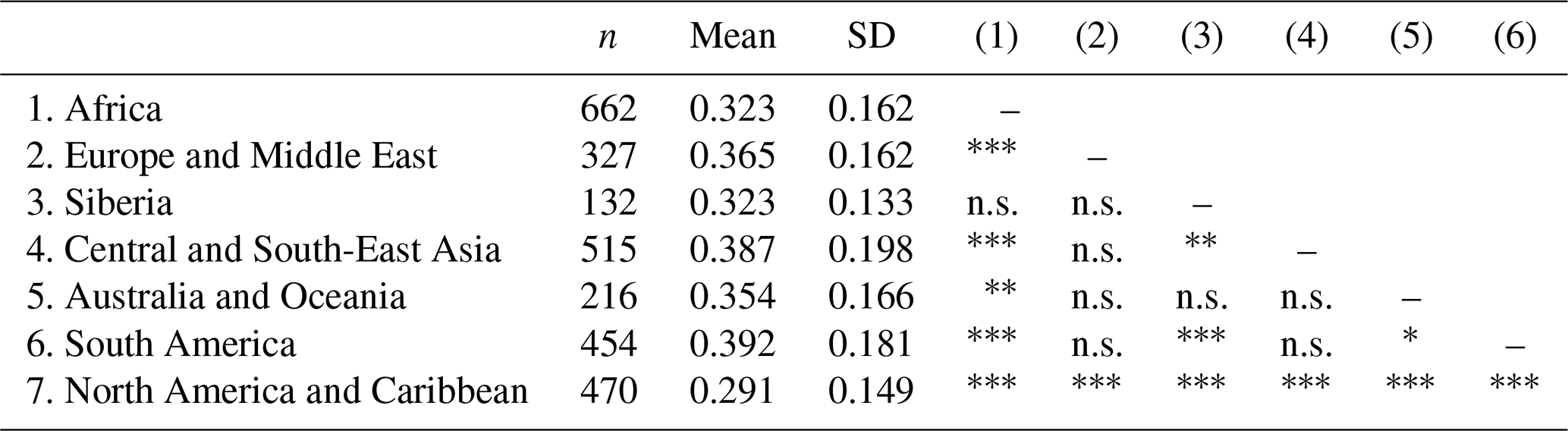
Note: ∗ p<0.05, p<0.01, p<0.001. n.s.: p>0.05.
Table A5Summary statistics and pairwise comparisons of how MAI-500 (the model agreement index of GFPLAIN, GAR-500, and JRC-500) varies with different river stream orders. A Kruskal–Wallis test showed that there is a significant difference in model agreement between the river stream orders (H(3)=101, p<0.001). The pairwise comparisons, for detecting significant differences between the stream orders, have been conducted using the Wilcoxon rank-sum test with continuity correction.
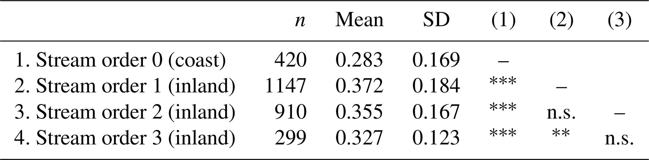
Note: ∗ p<0.05, p<0.01, p<0.001. n.s.: p>0.05.
Table A6Summary statistics and pairwise comparisons of how MAI-500 (the model agreement index of GFPLAIN, GAR-500, and JRC-500) varies with the freshwater major habitat types that spatially dominate the river basin. A Kruskal–Wallis test showed that there is a significant difference in model agreement between freshwater habitat types (H(10)=478, p<0.001). The pairwise comparisons, for detecting significant differences between the habitat types, have been conducted using the Wilcoxon rank-sum test with continuity correction.
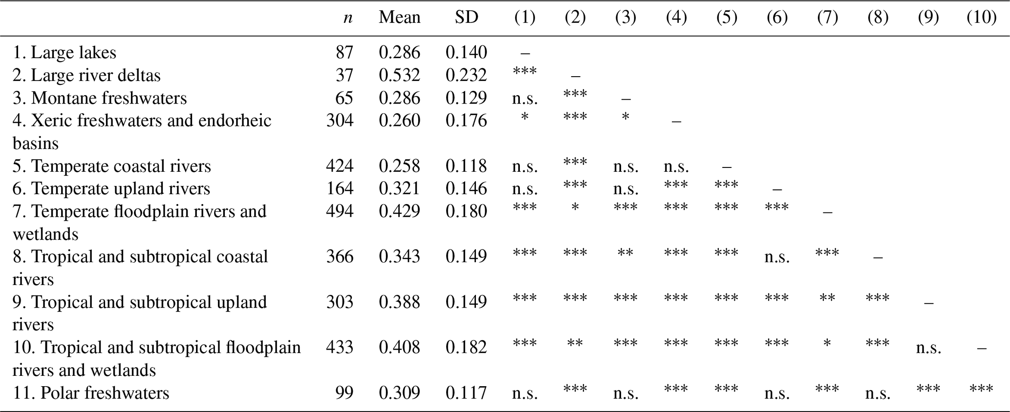
Note: ∗ p<0.05, p<0.01, p<0.001. n.s.: p>0.05.
Table A7Total country population (millions) using data from the World Bank (The World Bank, 2021a), GHS, HRSL, and WorldPop for 26 countries.
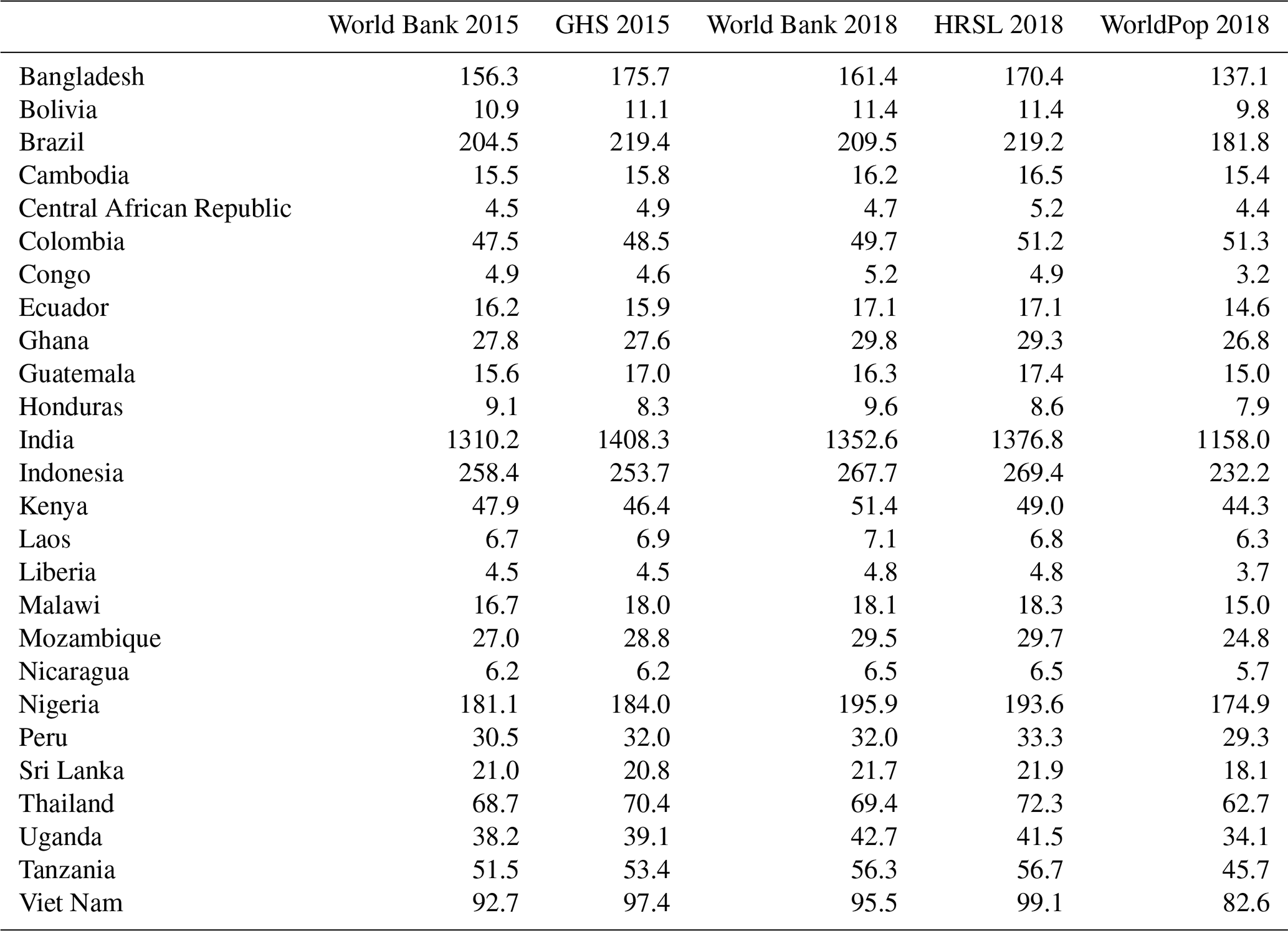
Table A8Total land area and flood-prone area (square kilometres) using GFPLAIN, JRC-100, JRC-500, GAR-100, and GAR-500. Land area is the total country area minus surface water area, given by the water mask MOD44W. The percentage of country area that is normally occurring surface water is less than 5 % for all countries, except Uganda with Lake Victoria (15 %) and Malawi with Lake Malawi (20 %).
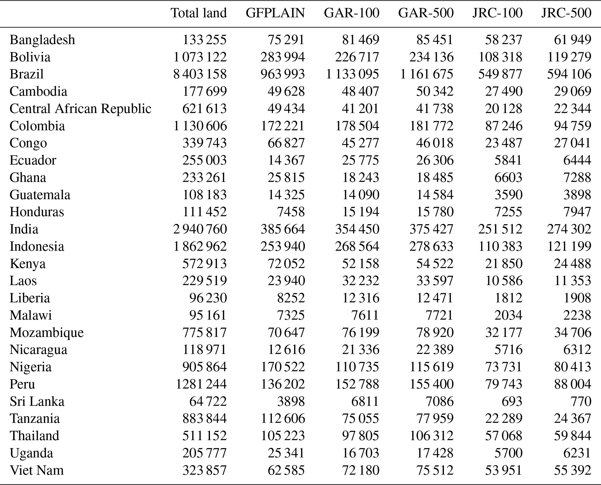
Table A9Population estimates within flood-prone areas (millions) intersecting GFPLAIN, GAR-500, and JRC-500 with GHS, HRSL, and WorldPop for 26 countries.
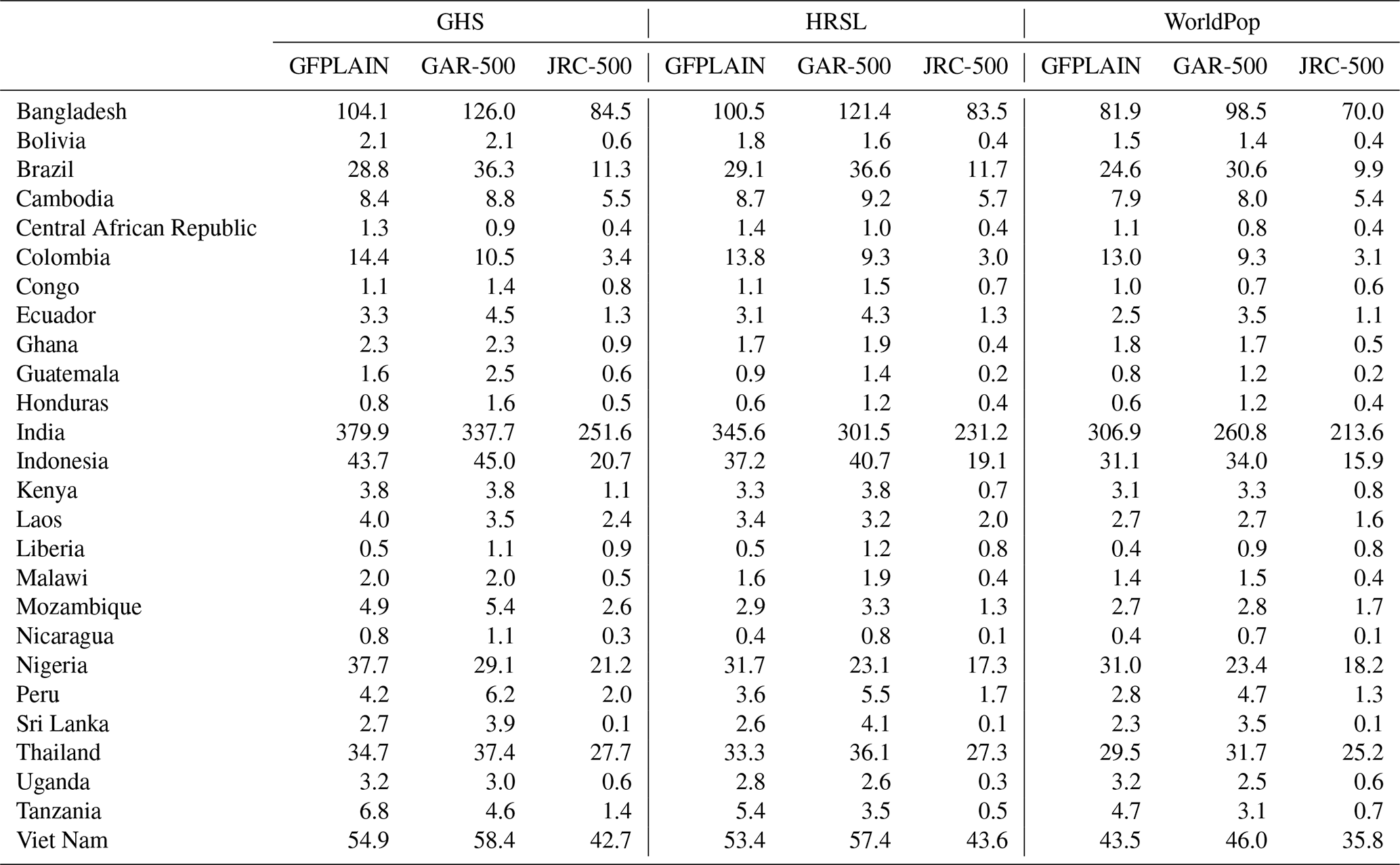
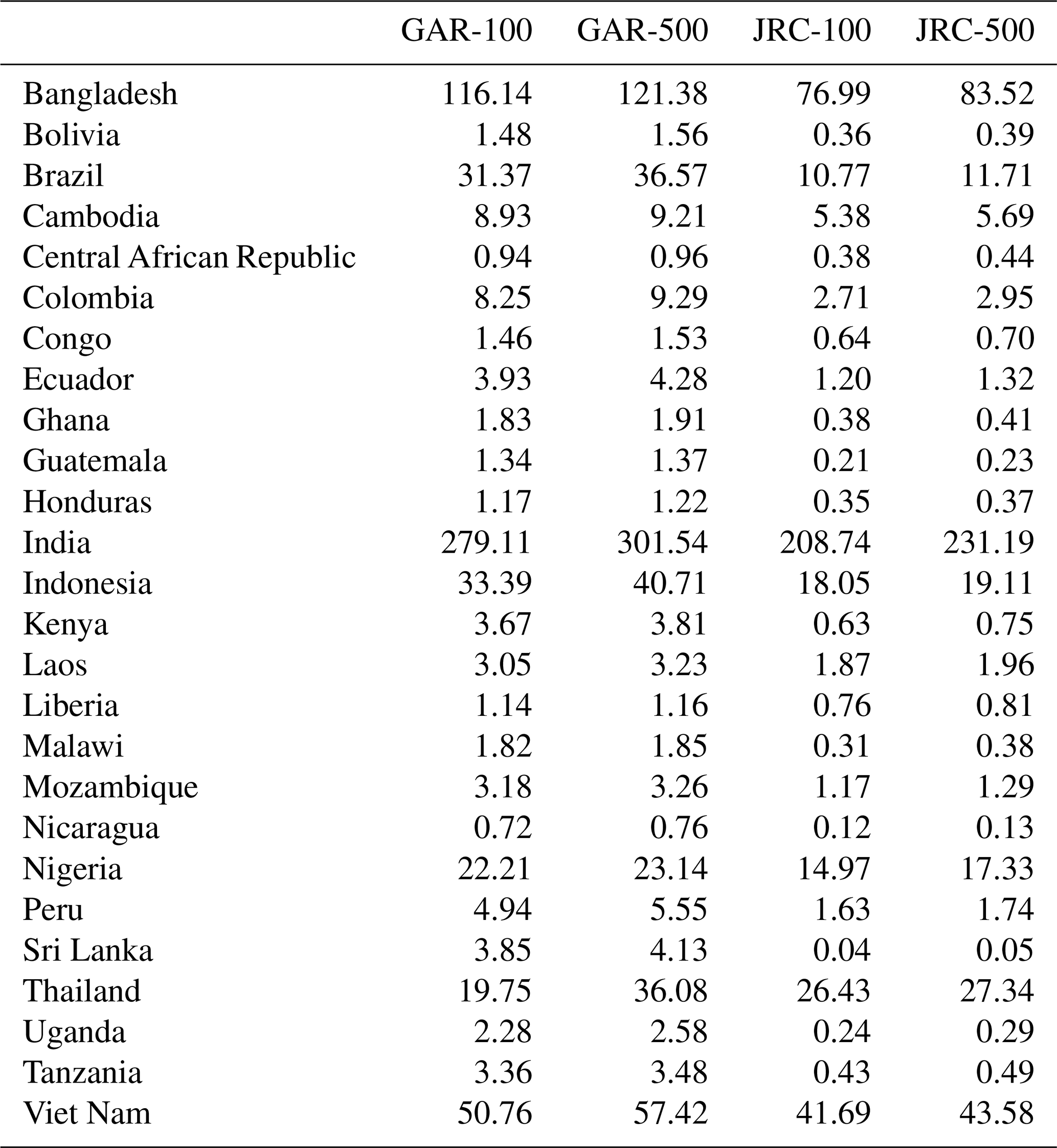
Table A10Population estimates within flood-prone areas (millions) using a return period of 100 years compared to 500 years, intersecting GAR and JRC with the HRSL population dataset.
The geospatial analysis has primarily been conducted in Google Earth Engine, and the statistical analysis has been conducted in R. The corresponding codes are made available upon request.
The floodplain layer GFPLAIN250m is available at https://doi.org/doi:10.6084/m9.figshare.6665165.v1 (Nardi and Annis, 2018). The JRC Flood Hazard Map of the World is available at http://data.europa.eu/89h/jrc-floods-floodmapgl_rp500y-tif and http://data.europa.eu/89h/jrc-floods-floodmapgl_rp100y-tif (Dottori et al., 2016b, c). The Global Assessment Report 2015 flood hazard maps can be accessed via the PREVIEW Global Risk Data Platform https://preview.grid.unep.ch/ (CIMA Research Foundation and UNEP, 2015). HydroBASINS and HydroATLAS are available at https://www.hydrosheds.org/ (HydroBasins; Lehner and Grill, 2013) and https://doi.org/10.6084/m9.figshare.9890531.v1 (HydroATLAS: Lehner et al., 2019). The remaining datasets were all accessed through the Google Earth Engine Data Catalog (Gorelick et al., 2017).
-
Global Administrative Unit Layers:
ee.FeatureCollection(“FAO/GAUL/2015/level0”) -
Global Human Settlement population grid:
ee.ImageCollection(“JRC/GHSL/P2016/POP_GPW_GLOBE
_V1”) -
High Resolution Settlement Layer:
ee.ImageCollection(“projects/sat-io/open-datasets/hrslpop”) -
HydroBASINS:
ee.FeatureCollection(“WWF/HydroSHEDS/v1/Basins/hybas
_5”) -
MOD44W Land Water Mask:
ee.Image(“MODIS/MOD44W/MOD44W_005_2000_02
_24”) -
WorldPop: ee.ImageCollection(“WorldPop/GP/100m/pop”)
SL, JM, LB, and GDB contributed to the study conceptualizations. SL designed and carried out the data analysis and visualization. SL prepared the original manuscript draft. JM, LB, and GDB reviewed and edited the manuscript.
The contact author has declared that neither they nor their co-authors have any competing interests.
Publisher's note: Copernicus Publications remains neutral with regard to jurisdictional claims in published maps and institutional affiliations.
The authors acknowledge Fernando Nardi and Antonio Annis for providing the floodplain layer GFPLAIN250m and the European Commission's Joint Research Centre and the UN Environment Programme for providing the global flood hazard layers. We also acknowledge the European Commission, Facebook Connectivity Lab with Columbia University, and WorldPop for providing the population layers. We are furthermore grateful to Francesco Dottori and the anonymous referee for providing helpful reviews that enriched the final paper.
This research has been supported by the H2020 programme of the European Research Council (grant no. 771678).
This paper was edited by Olga Petrucci and reviewed by Francesco Dottori and one anonymous referee.
Abell, R., Thieme, M. L., Revenga, C., Bryer, M., Kottelat, M., Bogutskaya, N., Coad, B., Mandrak, N., Balderas, S. C., Bussing, W., Stiassny, M. L. J., Skelton, P., Allen, G. R., Unmack, P., Naseka, A., Ng, R., Sindorf, N., Robertson, J., Armijo, E., Higgins, J. V, Heibel, T. J., Wikramanayake, E., Olson, D., López, H. L., Reis, R. E., Lundberg, J. G., Sabaj Pérez, M. H., and Petry, P.: Freshwater Ecoregions of the World: A New Map of Biogeographic Units for Freshwater Biodiversity Conservation, BioScience, 58, 403–414, https://doi.org/10.1641/B580507, 2008.
Aerts, J. P. M., Uhlemann-Elmer, S., Eilander, D., and Ward, P. J.: Comparison of estimates of global flood models for flood hazard and exposed gross domestic product: a China case study, Nat. Hazards Earth Syst. Sci., 20, 3245–3260, https://doi.org/10.5194/nhess-20-3245-2020, 2020.
Akhter, F., Mazzoleni, M., and Brandimarte, L.: Analysis of 220 Years of Floodplain Population Dynamics in the US at Different Spatial Scales, Water, 13, 141, https://doi.org/10.3390/w13020141, 2021.
Alfieri, L., Bisselink, B., Dottori, F., Naumann, G., de Roo, A., Salamon, P., Wyser, K., and Feyen, L.: Global projections of river flood risk in a warmer world, Earths Future, 5, 171–182, https://doi.org/10.1002/2016EF000485, 2017.
Annis, A., Nardi, F., Morrison, R. R., and Castelli, F.: Investigating hydrogeomorphic floodplain mapping performance with varying DTM resolution and stream order, Hydrol. Sci. J., 64, 525–538, https://doi.org/10.1080/02626667.2019.1591623, 2019.
Anselin, L.: Local Indicators of Spatial Association—LISA, Geogr. Anal., 27, 93–115, https://doi.org/10.1111/j.1538-4632.1995.tb00338.x, 1995.
Anselin, L., Syabri, I., and Kho, Y.: GeoDa: An Introduction to Spatial Data Analysis, Geogr. Anal., 38, 5–22, https://doi.org/10.1111/j.0016-7363.2005.00671.x, 2006.
Aronica, G., Bates, P. D., and Horritt, M. S.: Assessing the uncertainty in distributed model predictions using observed binary pattern information within GLUE, Hydrol. Process., 16, 2001–2016, https://doi.org/10.1002/hyp.398, 2002.
Bartholomé, E. and Belward, A. S.: GLC2000: a new approach to global land cover mapping from Earth observation data, Int. J. Remote Sens., 26, 1959–1977, https://doi.org/10.1080/01431160412331291297, 2005.
Bates, P. D. and De Roo, A. P. J.: A simple raster-based model for flood inundation simulation, J. Hydrol., 236, 54–77, https://doi.org/10.1016/S0022-1694(00)00278-X, 2000.
Beck, H., Zimmermann, N., McVicar, T., Vergopolan, N., Berg, A., and Wood, E.: Present and future Köppen-Geiger climate classification maps at 1 km resolution, Sci. Data, 5, 180214, https://doi.org/10.1038/sdata.2018.214, 2018.
Benjamini, Y. and Hochberg, Y.: Controlling the False Discovery Rate: A Practical and Powerful Approach to Multiple Testing, J. R. Stat. Soc. Ser. B, 57, 289–300, http://www.jstor.org/stable/2346101 (last access: 1 March 2021), 1995.
Bernhofen, M. V., Whyman, C., Trigg, M. A., Sleigh, P. A., Smith, A. M., Sampson, C. C., Yamazaki, D., Ward, P. J., Rudari, R., Pappenberger, F., Dottori, F., Salamon, P., and Winsemius, H. C.: A first collective validation of global fluvial flood models for major floods in Nigeria and Mozambique, Environ. Res. Lett., 13, 104007, https://doi.org/10.1088/1748-9326/aae014, 2018.
Bhowmik, N. G.: Hydraulic geometry of floodplains, J. Hydrol., 68, 369–401, https://doi.org/10.1016/0022-1694(84)90221-X, 1984.
Blöschl, G., Sivapalan, M., Wagener, T., Viglione, A., and Savenije, H. (Eds.): Runoff Prediction in Ungauged Basins: Synthesis across Processes, Places and Scales, Cambridge University Press, Cambridge, UK, https://doi.org/10.1017/CBO9781139235761, 2013.
Carroll, M. L., Townshend, J. R., DiMiceli, C. M., Noojipady, P., and Sohlberg, R. A.: A new global raster water mask at 250 m resolution, Int. J. Digit. Earth, 2, 291–308, https://doi.org/10.1080/17538940902951401, 2009.
Ceola, S., Laio, F., and Montanari, A.: Satellite nighttime lights reveal increasing human exposure to floods worldwide, Geophys. Res. Lett., 41, 7184–7190, https://doi.org/10.1002/2014GL061859, 2014.
Centre for Research on the Epidemiology of Disasters (CRED) and United Nations Office for Disaster Risk Reduction (UNDRR): Human Cost of Disasters: An Overview of the Last 20 Years (2000–2019), United Nations, https://cred.be/sites/default/files/CRED-Disaster-Report-Human-Cost2000-2019.pdf (last access: 13 February 2021), 2020.
CIESIN – Center for International Earth Science Information Network, Columbia University: Gridded Population of the World, Version 4 (GPWv4): Population Count, NASA Socioeconomic Data and Applications Center (SEDAC) [data set], https://doi.org/10.7927/H4X63JVC, 2016a.
CIESIN – Center for International Earth Science Information Network, Columbia University: Gridded Population of the World, Version 4 (GPWv4): Population Density, NASA Socioeconomic Data and Applications Center (SEDAC) [data set], https://doi.org/10.7927/H4NP22DQ, 2016b.
CIMA Foundation – Centro Internazionale in Monitoraggio Ambientale Foundation: Improvement of the Global Flood Model for the GAR15, Background Paper prepared for the 2015 Global Assessment Report on Disaster Risk Reduction, UNISDR, Geneva, Switzerland, 2015.
CIMA Research Foundation and UNEP: Flood Hazard Model for the Global Assessment Report 2015, PREVIEW Global Risk Data Platform, UNEP [data set], available at: https://preview.grid.unep.ch/ (last access: 3 February 2021), 2015.
Di Baldassarre, G., Nardi, F., Annis, A., Odongo, V., Rusca, M., and Grimaldi, S.: Brief communication: Comparing hydrological and hydrogeomorphic paradigms for global flood hazard mapping, Nat. Hazards Earth Syst. Sci., 20, 1415–1419, https://doi.org/10.5194/nhess-20-1415-2020, 2020.
Dodov, B. A. and Foufoula-Georgiou, E.: Floodplain morphometry extraction from a high-resolution digital elevation model: a simple algorithm for regional analysis studies, IEEE Geosci. Remote S., 3, 410–413, https://doi.org/10.1109/LGRS.2006.874161, 2006.
Döll, P., Kaspar, F., and Lehner, B.: A global hydrological model for deriving water availability indicators: model tuning and validation, J. Hydrol., 270, 105–134, https://doi.org/10.1016/S0022-1694(02)00283-4, 2003.
Dottori, F., Salamon, P., Bianchi, A., Alfieri, L., Hirpa, F. A., and Feyen, L.: Development and evaluation of a framework for global flood hazard mapping, Adv. Water Resour., 94, 87–102, https://doi.org/10.1016/j.advwatres.2016.05.002, 2016a.
Dottori, F., Alfieri, L., Salamon, P., Bianchi, A., Feyen, L., and Hirpa, F.: Flood hazard map of the World – 500-year return period, European Commission, Joint Research Centre (JRC) [data set], available at: http://data.europa.eu/89h/jrc-floods-floodmapgl_rp500y-tif (last access: 3 February 2021), 2016b.
Dottori, F., Alfieri, L., Salamon, P., Bianchi, A., Feyen, L., and Hirpa, F.: Flood hazard map of the World – 100-year return period, European Commission, Joint Research Centre (JRC) [data set], available at: http://data.europa.eu/89h/jrc-floods-floodmapgl_rp100y-tif (last access: 3 February 2021), 2016c.
Ehrlich, D., Melchiorri, M., Florczyk, A., Pesaresi, M., Kemper, T., Corbane, C., Freire, S., Schiavina, M., and Siragusa, A.: Remote Sensing Derived Built-Up Area and Population Density to Quantify Global Exposure to Five Natural Hazards over Time, Remote Sens., 10, 1378, https://doi.org/10.3390/rs10091378, 2018.
ESA: Land Cover CCI Product User Guide Version 2, Tech. Rep., available at: http://maps.elie.ucl.ac.be/CCI/viewer/download/ESACCI-LC-Ph2-PUGv2_2.0.pdf (last access: 29 September 2021), 2017.
Facebook Connectivity Lab and Center for International Earth Science Information Network (CIESIN) Columbia University: High Resolution Settlement Layer (HRSL), Columbia University [data set], https://ciesin.columbia.edu/data/hrsl (last access: 3 February 2021), 2016.
FAO UN – Food and Agriculture Organization of the United Nations: Global Administrative Unit Layers 2015, Country Boundaries, Google Earth Engine [data set], https://developers.google.com/earth-engine/datasets/catalog/FAO_GAUL_2015_level0 (last access: 3 February 2021), 2015.
Farr, T. G., Rosen, P. A., Caro, E., Crippen, R., Duren, R., Hensley, S., Kobrick, M., Paller, M., Rodriguez, E., Roth, L., Seal, D., Shaffer, S., Shimada, J., Umland, J., Werner, M., Oskin, M., Burbank, D., and Alsdorf, D. E.: The Shuttle Radar Topography Mission, Rev. Geophys., 45, RG2004, https://doi.org/10.1029/2005RG000183, 2007.
Foster, K. R., Vecchia, P., and Repacholi, M. H.: Science and the Precautionary Principle, Science, 288, 979–981, https://doi.org/10.1126/science.288.5468.979, 2000.
Gaughan, A. E., Stevens, F. R., Linard, C., Jia, P., and Tatem, A. J.: High Resolution Population Distribution Maps for Southeast Asia in 2010 and 2015, PLoS One, 8, e55882, https://doi.org/10.1371/journal.pone.0055882, 2013.
Gorelick, N., Hancher, M., Dixon, M., Ilyushchenko, S., Thau, D., and Moore, R.: Google Earth Engine: Planetary-scale geospatial analysis for everyone, Remote Sens. Environ., 202, 18–27, https://doi.org/10.1016/j.rse.2017.06.031, 2017.
Gruber, S.: Derivation and analysis of a high-resolution estimate of global permafrost zonation, The Cryosphere, 6, 221–233, https://doi.org/10.5194/tc-6-221-2012, 2012.
Guha-Sapir, D., Below, R., and Hoyois, P.: EM-DAT International disaster database, Centre for Research on the Epidemiology of Disasters (CRED) [data set], https://emdat.be (last access: 1 April 2020), 2014.
Hall, D. K. and Riggs, G. A.: MODIS/Aqua Snow Cover Daily L3 Global 500 m SIN Grid, Version 6. [2002–2015], National Snow and Ice Data Center (NSIDC) [data set], https://doi.org/10.5067/MODIS/MYD10A1.006, 2016.
Harell Jr., F. E. and Dupont, C.: Hmisc: Harrell Miscellaneous, The Comprehensive R Archive Network (CRAN) [R package], https://cran.r-project.org/web/packages/Hmisc/, last access: 1 March 2021.
Hawker, L., Neal, J., Tellman, B., Liang, J., Schumann, G., Doyle, C., Sullivan, J. A., Savage, J., and Tshimanga, R.: Comparing earth observation and inundation models to map flood hazards, Environ. Res. Lett., 15, 124032, https://doi.org/10.1088/1748-9326/abc216, 2020.
Hijmans, R. J., Cameron, S. E., Parra, J. L., Jones, P. G., and Jarvis, A.: Very high resolution interpolated climate surfaces for global land areas, Int. J. Climatol., 25, 1965–1978, https://doi.org/10.1002/joc.1276, 2005.
Hollander, M. and Wolfe, D. A.: Nonparametric Statistical Methods, Wiley, New York, USA, 1973.
Jongman, B., Ward, P. J., and Aerts, J. C. J. H.: Global exposure to river and coastal flooding: Long term trends and changes, Global Environ. Chang., 22, 823–835, https://doi.org/10.1016/j.gloenvcha.2012.07.004, 2012.
Kidd, C., Becker, A., Huffman, G. J., Muller, C. L., Joe, P., Skofronick-Jackson, G., and Kirschbaum, D. B.: So, how much of the Earth's surface is covered by rain gauges?, B. Am. Meteorol. Soc., 98, 69–78, https://doi.org/10.1175/BAMS-D-14-00283.1, 2017.
Kummu, M., Taka, M., and Guillaume, J. H. A.: Gridded global datasets for Gross Domestic Product and Human Development Index over 1990–2015, Sci. Data, 5, 180004, https://doi.org/10.1038/sdata.2018.4, 2018.
Lehner, B.: HydroBASINS Technical Documentation Version 1.c, Report, available at: https://www.hydrosheds.org/images/inpages/HydroBASINS_TechDoc_v1c.pdf (last access: 3 February 2021), 2014.
Lehner, B. and Grill, G.: Global river hydrography and network routing: Baseline data and new approaches to study the world's large river systems, Hydrol. Process., 27, 2171–2186, https://doi.org/10.1002/hyp.9740, 2013a.
Lehner, B. and Grill, G.: HydroBasins version 1 level 5, HydroSHEDS [data set], available at: https://hydrosheds.org (last access: 15 March 2021), 2013b.
Lehner, B., Linke, S., and Thieme, M.: HydroATLAS version 1.0, Figshare [data set], https://doi.org/10.6084/m9.figshare.9890531.v1, 2019.
Leyk, S., Gaughan, A. E., Adamo, S. B., de Sherbinin, A., Balk, D., Freire, S., Rose, A., Stevens, F. R., Blankespoor, B., Frye, C., Comenetz, J., Sorichetta, A., MacManus, K., Pistolesi, L., Levy, M., Tatem, A. J., and Pesaresi, M.: The spatial allocation of population: a review of large-scale gridded population data products and their fitness for use, Earth Syst. Sci. Data, 11, 1385–1409, https://doi.org/10.5194/essd-11-1385-2019, 2019.
Linard, C., Gilbert, M., Snow, R. W., Noor, A. M., and Tatem, A. J.: Population distribution, settlement patterns and accessibility across Africa in 2010, PLoS One, 7, e31743, https://doi.org/10.1371/journal.pone.0031743, 2012.
Lindersson, S., Brandimarte, L., Mård, J., and Di Baldassarre, G.: A review of freely accessible global datasets for the study of floods, droughts and their interactions with human societies, WIREs Water, 7, e1424, https://doi.org/10.1002/wat2.1424, 2020.
Linke, S., Lehner, B., Ouellet Dallaire, C., Ariwi, J., Grill, G., Anand, M., Beames, P., Burchard-Levine, V., Maxwell, S., Moidu, H., Tan, F., and Thieme, M.: Global hydro-environmental sub-basin and river reach characteristics at high spatial resolution, Sci. Data, 6, 283, https://doi.org/10.1038/s41597-019-0300-6, 2019.
Lloyd, C. T., Sorichetta, A., and Tatem, A. J.: High resolution global gridded data for use in population studies, Sci. Data, 4, 170001, https://doi.org/10.1038/sdata.2017.1, 2017.
Manfreda, S., Nardi, F., Samela, C., Grimaldi, S., Taramasso, A. C., Roth, G., and Sole, A.: Investigation on the use of geomorphic approaches for the delineation of flood prone areas, J. Hydrol., 517, 863–876, https://doi.org/10.1016/j.jhydrol.2014.06.009, 2014.
Mazzoleni, M., Mård, J., Rusca, M., Odongo, V., Lindersson, S., and Di Baldassarre, G.: Floodplains in the Anthropocene: A global analysis of the interplay between human population, built environment and flood severity, Water Resour. Res., 57, e2020WR027744, https://doi.org/10.1029/2020WR027744, 2020.
Nardi, F. and Annis, A.: GFPLAIN250m, Figshare [data set], https://doi.org/10.6084/m9.figshare.6665165.v1, 2018.
Nardi, F., Vivoni, E. R., and Grimaldi, S.: Investigating a floodplain scaling relation using a hydrogeomorphic delineation method, Water Resour. Res., 42, W09409, https://doi.org/10.1029/2005WR004155, 2006.
Nardi, F., Morrison, R. R., Annis, A., and Grantham, T. E.: Hydrologic scaling for hydrogeomorphic floodplain mapping: Insights into human-induced floodplain disconnectivity, River Res. Appl., 34, 675–685, https://doi.org/10.1002/rra.3296, 2018.
Nardi, F., Annis, A., Di Baldassarre, G., Vivoni, E. R., and Grimaldi, S.: GFPLAIN250m, a global high-resolution dataset of Earth's floodplains, Sci. Data, 6, 180309, https://doi.org/10.1038/sdata.2018.309, 2019.
Ouellet Dallaire, C., Lehner, B., Sayre, R., and Thieme, M.: A multidisciplinary framework to derive global river reach classifications at high spatial resolution, Environ. Res. Lett., 14, 024003, https://doi.org/10.1088/1748-9326/aad8e9, 2019.
Pappenberger, F., Frodsham, K., Beven, K., Romanowicz, R., and Matgen, P.: Fuzzy set approach to calibrating distributed flood inundation models using remote sensing observations, Hydrol. Earth Syst. Sci., 11, 739–752, https://doi.org/10.5194/hess-11-739-2007, 2007.
Pesaresi, M. and Freire, S.: GHS-SMOD R2016A – GHS settlement grid, following the REGIO model 2014 in application to GHSL Landsat and CIESIN GPW v4-multitemporal (1975–1990–2000–2015), European Commission, Joint Research Centre (JRC) [data set], http://data.europa.eu/89h/jrc-ghsl-ghs_smod_pop_globe_r2016a (last access: 2 April 2021), 2016.
Ramankutty, N., Evan, A. T., Monfreda, C., and Foley, J. A.: Farming the planet: 1. Geographic distribution of global agricultural lands in the year 2000, Global Biogeochem. Cy., 22, GB1003, https://doi.org/10.1029/2007GB002952, 2008.
Raup, B., Racoviteanu, A., Jodha, S., Khalsa, S., Helm, C., Armstrong, R., and Arnaud, Y.: The GLIMS geospatial glacier database: A new tool for studying glacier change, Global Planet. Change, 56, 101–110, https://doi.org/10.1016/j.gloplacha.2006.07.018, 2007.
R Core Team: R: A language and environment for statistical computing, R Foundation for Statistical Computing, Vienna, Austria, http://r-project.org (last access: 1 March 2021), 2014.
Reuter, H. I., Nelson, A., and Jarvis, A.: An evaluation of void-filling interpolation methods for SRTM data, Int. J. Geogr. Inf. Sci., 21, 983–1008, https://doi.org/10.1080/13658810601169899, 2007.
Robinson, N., Regetz, J., and Guralnick, R. P.: EarthEnv-DEM90: A nearly-global, void-free, multi-scale smoothed, 90 m digital elevation model from fused ASTER and SRTM data, ISPRS J. Photogramm., 87, 57–67, https://doi.org/10.1016/j.isprsjprs.2013.11.002, 2014.
Sampson, C. C., Smith, A. M., Bates, P. D., Neal, J. C., Alfieri, L., and Freer, J. E.: A high-resolution global flood hazard model, Water Resour. Res., 51, 7358–7381, https://doi.org/10.1002/2015WR016954, 2015.
Schiavina, M., Freire, S., and Macmanus, K.: GHS-POP R2019A – GHS population grid multitemporal (1975–1990–2000–2015), European Commission, Joint Research Centre (JRC) [data set], https://doi.org/10.2905/0C6B9751-A71F-4062-830B-43C9F432370F, 2019.
Schumann, G., Bates, P. D., Horritt, M. S., Matgen, P., and Pappenberger, F.: Progress in integration of remote sensing-derived flood extent and stage data and hydraulic models, Rev. Geophys., 47, RG4001, https://doi.org/10.1029/2008RG000274, 2009.
Siebert, S., Kummu, M., Porkka, M., Döll, P., Ramankutty, N., and Scanlon, B. R.: A global data set of the extent of irrigated land from 1900 to 2005, Hydrol. Earth Syst. Sci., 19, 1521–1545, https://doi.org/10.5194/hess-19-1521-2015, 2015.
Smith, A., Bates, P. D., Wing, O., Sampson, C., Quinn, N., and Neal, J.: New estimates of flood exposure in developing countries using high-resolution population data, Nat. Commun., 10, 1–7, https://doi.org/10.1038/s41467-019-09282-y, 2019.
Sorichetta, A., Hornby, G. M., Stevens, F. R., Gaughan, A. E., Linard, C., and Tatem, A. J.: High-resolution gridded population datasets for Latin America and the Caribbean in 2010, 2015, and 2020, Sci. Data, 2, 150045, https://doi.org/10.1038/sdata.2015.45, 2015.
Spearman, C.: The Proof and Measurement of Association between Two Things, Am. J. Psychol., 15, 72–101, https://doi.org/10.2307/1412159, 1904.
Tatem, A. J.: WorldPop, open data for spatial demography, Sci. Data, 4, 170004, https://doi.org/10.1038/sdata.2017.4, 2017.
Tavares da Costa, R., Manfreda, S., Luzzi, V., Samela, C., Mazzoli, P., Castellarin, A., and Bagli, S.: A web application for hydrogeomorphic flood hazard mapping, Environ. Modell. Softw., 118, 172–186, https://doi.org/10.1016/j.envsoft.2019.04.010, 2019.
Tellman, B., Sullivan, J. A., Kuhn, C., Kettner, A. J., Doyle, C. S., Brakenridge, G. R., Erickson, T. A., and Slayback, D. A.: Satellite imaging reveals increased proportion of population exposed to floods, Nature, 596, 80–86, https://doi.org/10.1038/s41586-021-03695-w, 2021.
The World Bank: World Development Indicators – Population, total, World Bank Data Bank [data set], https://data.worldbank.org/indicator/SP.POP.TOTL (last access: 17 February 2021), 2021a.
The World Bank: World development indicators – GNI per capita, Atlas method, World Bank DataBank [data set], http://data.worldbank.org/indicator/NY.GNP.PCAP.CD (last access: 17 February 2021), 2021b.
Tiecke, T. G., Liu, X., Zhang, A., Gros, A., Li, N., Yetman, G., Kilic, T., Murray, S., Blankespoor, B., Prydz, E. B., and Dang, H. A. H.: Mapping the world population one building at a time, arXiv:1712.05839, https://doi.org/10.1596/33700, 2017.
Trigg, M. A., Birch, C. E., Neal, J. C., Bates, P. D., Smith, A., Sampson, C. C., Yamazaki, D., Hirabayashi, Y., Pappenberger, F., Dutra, E., Ward, P. J., Winsemius, H. C., Salamon, P., Dottori, F., Rudari, R., Kappes, M. S., Simpson, A. L., Hadzilacos, G., and Fewtrell, T. J.: The credibility challenge for global fluvial flood risk analysis, Environ. Res. Lett., 11, 94014, https://doi.org/10.1088/1748-9326/11/9/094014, 2016.
UNISDR – United Nations Office for Disaster Risk Reduction: Making Development Sustainable: The Future of Disaster Risk Management, Global Assessment Report on Disaster Risk Reduction. UNISDR, Geneva, Switzerland, 2015.
UN SDSN – United Nations Sustainable Development Solutions Network: Leaving no one off the map: a guide for gridded population data for sustainable development, UN SDSN TReNDS, New York, USA, 2020.
Ward, P. J., Jongman, B., Salamon, P., Simpson, A., Bates, P., De Groeve, T., Muis, S., De Perez, E. C., Rudari, R., Trigg, M. A., and Winsemius, H. C.: Usefulness and limitations of global flood risk models, Nat. Clim. Change, 5, 712–715, https://doi.org/10.1038/nclimate2742, 2015.
Ward, P. J., Blauhut, V., Bloemendaal, N., Daniell, J. E., de Ruiter, M. C., Duncan, M. J., Emberson, R., Jenkins, S. F., Kirschbaum, D., Kunz, M., Mohr, S., Muis, S., Riddell, G. A., Schäfer, A., Stanley, T., Veldkamp, T. I. E., and Winsemius, H. C.: Review article: Natural hazard risk assessments at the global scale, Nat. Hazards Earth Syst. Sci., 20, 1069–1096, https://doi.org/10.5194/nhess-20-1069-2020, 2020.
Wei, T. and Simko, V.: Corrplot: Visualization of a Correlation Matrix, The Comprehensive R Archive Network (CRAN) [R package], https://cran.r-project.org/web/packages/corrplot/ (last access: 1 March 2021), 2017.
Winsemius, H. C., Aerts, J. C. J. H., van Beek, L. P. H., Bierkens, M. F. P., Bouwman, A., Jongman, B., Kwadijk, J. C. J., Ligtvoet, W., Lucas, P. L., van Vuuren, D. P., and Ward, P. J.: Global drivers of future river flood risk, Nat. Clim. Change, 6, 381–385, https://doi.org/10.1038/nclimate2893, 2016.
Wright, J. K.: A Method of Mapping Densities of Population: With Cape Cod as an Example, Geogr. Rev., 26, 103–110, https://doi.org/10.2307/209467, 1936.
WWF and TNC: Freshwater Ecoregions of the World – Major Habitat Types, https://www.feow.org/global-maps/major-habitat-types (last access: 16 April 2021), 2019.
Yamazaki, D., Kanae, S., Kim, H., and Oki, T.: A physically based description of floodplain inundation dynamics in a global river routing model, Water Resour. Res., 47, W04501, https://doi.org/10.1029/2010WR009726, 2011.
Zischg, A. P. and Bermúdez, M.: Mapping the sensitivity of population exposure to changes in flood magnitude: prospective application from local to global scale, Front. Earth Sci., 8, 390, https://doi.org/10.3389/feart.2020.534735, 2020.
Zomer, R. J., Trabucco, A., Bossio, D. A., and Verchot, L. V: Climate change mitigation: A spatial analysis of global land suitability for clean development mechanism afforestation and reforestation, Agric. Ecosyst. Environ., 126, 67–80, https://doi.org/10.1016/j.agee.2008.01.014, 2008.