the Creative Commons Attribution 4.0 License.
the Creative Commons Attribution 4.0 License.
 | 23 Jul 2021
Spatiotemporal heterogeneity of b values revealed by a data-driven approach for the 17 June 2019 MS 6.0 Changning earthquake sequence, Sichuan, China
Libo Han
Feng Long
Guijuan Lai
Fengling Yin
Jinmeng Bi
Zhengya Si
The spatiotemporal heterogeneity of b values has great potential for helping in understanding the seismogenic process and assessing seismic hazard. However, there is still much controversy about whether it exists or not, and an important reason is that the choice of subjective parameters has eroded the foundations of much research. To overcome this problem, we used a recently developed non-parametric method based on a data-driven concept to calculate b values. The major steps of this method include (1) performing a large number of Voronoi tessellations and Bayesian information criterion (BIC) value calculation, selecting the optimal models for the study area, and (2) using the ensemble median (Q2) and median absolute deviation (MAD) value to represent the final b value and its uncertainty. We investigated spatiotemporal variations in b values before and after the 2019 Changning MS=6.0 earthquake in the Sichuan Basin, China. The results reveal a spatial volume with low pre-mainshock b values near the mainshock source region, and its size corresponds roughly with the rupture area of the mainshock. The anomalously high pre-mainshock b values distributed in the NW direction of the epicenter were interpreted to be related to fluid invasion. The decreases in b values during the aftershock sequence along with the occurrences of several strong aftershocks imply that b values could be an indicator of the stress state. In addition, we found that although the distribution characteristics of b values obtained from different methods of investigation are qualitatively consistent, they differ significantly in terms of their specific values, suggesting that the best way to study the heterogeneous pattern of b values is in the joint dimension of space-time rather than separately in time and space. Overall, our study emphasizes the importance of b-value studies in assessing earthquake hazards.
- Article
(6425 KB) - Full-text XML
-
Supplement
(897 KB) - BibTeX
- EndNote


The Gutenberg–Richter b value describes the corresponding frequency–magnitude distribution (FMD) characteristics by reflecting the relative proportion of the frequency of large and small earthquakes within a given space-time range. It is considered to be related to the stress conditions in the Earth's crust (e.g., Wyss, 1973; Urbancic et al., 1992; Mori and Abercrombie, 1997; Toda et al., 1998), complexity of the fault trace (Stirling et al., 1996), and the extent of creep (Amelung and King, 1997) and other factors. Experimental studies in the laboratory have shown that a weak and less resistant environment under stress would produce a high b value, while materials that are more compact and more resistant under pressure do not fail, which leads to a reasonably low b value (Aktar et al., 2004). In the case where the material and structure are clarified, a decreasing b value is considered to be related to increasing stress (Scholz, 1968) or pore pressure diffusion (Hainzl and Fischer, 2002; Lei and Satoh, 2007). For the above reasons, the b value has been widely considered in seismogenic environment analysis and seismic hazard research.
Spatial and temporal heterogeneity is an important topic in b-value research, especially under the assumptions that the local b values are inversely dependent on the applied shear stress and that low b values (b<0.7) can reflect the existence of locked faults or asperities. Therefore, the spatial and temporal heterogeneity of b values is considered an important clue for forecasting the location and size of potentially large earthquakes (Wiemer and Wyss, 1997; Schorlemmer and Wiemer, 2005; Murru et al., 2007). Using the spatial heterogeneity of the b value to identify possible asperities has been performed in some cases, such as for the San Jacinto–Elsinore fault system in southern California (Wyss et al., 2000), the Parkfield segment of the San Andreas fault (Wiemer and Wyss, 1997), and the case study of the 2014 Parkfield M=6.0 earthquake (Schorlemmer and Wiemer, 2005).
A model named the Asperity Likelihood Model (ALM) based on the above assumptions has been developed and used to forecast future earthquakes (Wiemer and Schorlemmer, 2007; Gulia et al., 2010). Research on the temporal heterogeneity of b values mainly includes using b-value time variation in the early aftershock sequence and the constructed system of the foreshock traffic light system (FTLS) to evaluate the risk of larger subsequent aftershocks (Gulia and Wiemer, 2019).
However, some research results show that the apparent variability in b values is not significant in some cases (Del Pezzo et al., 2003). For example, Amorèse et al. (2010) systematically examined the variation in b values in southern California to the depth of the crust and found that the hypothesis was not statistically significant. By using a data-driven approach, Kamer and Hiemer (2015) show that the spatial b values in most locations in California are distributed within a very limited range (0.94±0.04–1.15±0.06), and the previously reported spatial b-value variation is overestimated and mainly due to the subjective choice of parameters. Besides, the spatial and temporal heterogeneity of b values is also considered to be due to the subjective arbitrariness of the calculation rules and the lack of statistical robustness (Kagan, 1999).
Based on the above viewpoints, the calculation reliability for research on the spatiotemporal heterogeneity of b values still needs to be solved, and the relationship between the spatiotemporal variation process of b values and the occurrence of strong earthquakes needs to be investigated for more earthquake cases. In this study, we will utilize data-driven b-value calculation methods that have been developed in recent years (Kamer and Hiemer, 2015; Nandan et al., 2017; Si and Jiang, 2019) for case studies of the 2019 Changning MS=6.0 earthquake in Sichuan, China.
In the traditional calculation of the Guttenberg–Richter magnitude–frequency b value, a fixed number of earthquakes (Hutton et al., 2010; Ogata, 2011) or a fixed minimum and maximum selection radius (Woessner and Wiemer, 2005) are generally used to select data and the maximum likelihood estimation is used to obtain b values. Because such calculations have strong subjectivity in their calculating rules, they have caused widespread controversy. The data-driven approaches to seismicity parameter calculation have been gradually developed in recent years (Sambridge et al., 2013; Kamer and Hiemer, 2015; Nandan et al., 2017; Si and Jiang, 2019) by using the Voronoi tessellation to create a large number of spatially random grids and covering the possibility of the segmentation of spatial regions, relying on the Bayesian information criterion (BIC) to select a part of the optimal models with the smallest BIC value and representing the final result of seismic activity parameters through the ensemble median value. Because the data-driven approach uses an automatic parametric calculation, it provides a possibility of solving the subjective problem of earthquake data selection.
Among those data-driven approaches, Si and Jiang (2019) developed a method using the continuous distribution function (hereafter referred to as the OK1993 model) given by Ogata and Katsura (1993), which has the advantage of simultaneously determining the minimum magnitude of completeness and obtaining b values. In this paper, we will use this approach to study the spatiotemporal heterogeneity of b values for the 2019 Changning MS=6.0 earthquake.
The OK1993 model uses the seismic detection rate function q(M) to describe the complete detection degree of earthquake events with different magnitudes in the magnitude–frequency distribution:
where M is the magnitude, the parameter μ represents the corresponding magnitude to the detection rate of 50 %, and σ indicates the corresponding magnitude range. The actual earthquake probability density function and the log-likelihood function of the OK1993 model can be expressed as
{M1, M2, …, Mn} in the above formula is the magnitude of a given series of observational events and the power exponent β=bln 10, The parameter [β, μ, σ] can be obtained by fitting the above formula using the maximum likelihood method. The Bayesian information criterion is adopted to calculate the corresponding BIC value and select the optimal models. Since each grid node is composed of spatial coordinates [x, y] and three parameters [β, μ, σ] in the OK1993 model, the total number of freedom degrees is in the entire study region.
The construction of the data-driven approach can be achieved by Voronoi tessellation with limited boundaries. Voronoi tessellation refers to a unique set of continuous polygon partitioning schemes {Pi, i=1, 2, …, n} given by a set of spatial nodes S={s1, s2, …, sn} in two-dimensional or three-dimensional space. The polygon , i≠j}, where dist(a, b) denotes the Euclidean distance between two points. Voronoi tessellation also benefits from the uniqueness of its spatial division, so it is widely used in computer science, political elections, and many other studies (Rubner et al., 2000; Svec et al., 2007). The calculation steps of the data-driven approach include the following: (1) randomly throwing a certain number of nodes into the study area and performing Voronoi meshing, with the number of grid nodes gradually increasing from 2 to 40, ensuring that the Voronoi tessellation covers the possibility of various spatial region segmentation by each number of grid nodes being randomly thrown 100 times; (2) calculating OK1993 model parameters and BIC values for … Voronoi cells obtained from 3900 tessellations (or spatial calculation models) and summing the BIC values of all the Voronoi cells obtained from each tessellation and using this as the basis for judging whether this spatial calculation model is the optimal model; and (3) selecting, among the 3900 spatial calculation models, 100 models (marked as best-100) with smaller BIC values as the optimal models and using the parameters [β, μ, σ] of the ensemble median (Q2) and median absolute deviation (MAD) as the final calculation results. The b value can be obtained by .
The maximum likelihood calculation of the OK1993 model parameter is not performed when the number of earthquakes contained in a Voronoi cell is N1<5, so the actual number of effective cells Nv obtained by each tessellation is used to distinguish the number of randomly thrown nodes. Although the value of N1 may affect the parameter fitting error in some polygons with a small number of events, considering that the OK1993 model in the form of a continuous distribution function has the advantage of obvious fit adaptability compared to the traditional linear frequency–magnitude distribution (FMD) function in a small number of data cases, this setting also ensures that the spatial division can obtain more polygon calculation results, and the final result of the parameters is expressed by the ensemble median value, so the effect of this method of value taking on the final result is minimal.
In the above calculation steps, the setting of the maximum number of nodes, the number of random throws, etc. has obvious subjectivity. However, due to the fact that the data-driven approach actually obtains a very stable final result when the number of divisions and the number of grid nodes are sufficient (Si and Jiang, 2019) – for example, when the maximum number of nodes is 100, each type of node is randomly thrown 1000 times – the final result obtained when 1000 optimal models are selected is almost the same as the result of this paper.
The 2019 Changning MS=6.0 earthquake sequence occurred in the basin–mountain junction in the southern margin of the Sichuan Basin, where the tectonic activity is relatively weak. The seismicity in the area is mainly controlled by folds and associated faults. The intensity of historically destructive earthquakes is low in the area where aftershocks extend. No earthquake with a magnitude above 5.0 had been recorded in this area before the Changning MS=6.0 earthquake. According to Yi et al. (2019), it is inferred that the occurrence of the Changning MS=6.0 earthquake sequence may be related to the Baixiangyan–Shizitan anticline and the Shuanghechang anticline and their associated fault activities. Figure 1 shows the study area of this paper. We will focus on the rectangular area A′B′C′D′ where the aftershock sequence mainly occurred and the rectangular area ABCD where the surrounding earthquakes are active.

Figure 1Distribution of seismicity in the Changning area. The red dots show the aftershocks of the Changning MS=6.0 earthquake, and the green dots indicate the earthquakes that occurred before the Changning MS=6.0 earthquake. Hexagonal stars mark the position of the mainshock and four aftershocks with magnitude no less than 5.0, and the corresponding focal mechanisms are marked. The dotted rectangular ABCD and A′B′C′D′ show the two spatial regions for calculating the b value and rotating the coordinate system, and the blue cross symbol gives the origin where the coordinate system is rotated. The blue triangles show the location of seismic stations that recorded these earthquakes, and the solid black lines represent active faults (He et al., 2019). The study region is shown in the location figure in the bottom left by a green rectangle.
We used earthquake catalogs and bulletins provided by the Sichuan Regional Seismic Network from 1 January 2009 to 17 July 2019. To obtain relatively reliable parameters such as the epicenter location and focal depth, the double-difference algorithm hypoDD (Waldhauser and Ellsworth, 2000) was used to relocate the earthquakes. Among the data we used are a total of 21 246 seismic events that meet the requirements of the hypoDD method with not less than four arrivals, including 516 649 P-wave arrivals and 506 809 S-wave arrivals, and 59 permanent seismic stations and temporary seismic stations are used which are located in Sichuan and the surrounding provinces. We used a 12-layer one-dimensional crustal velocity model (Xie et al., 2012) during the relocation. The ratio of VP to VS is set to 1.730.
A total of 18 371 earthquake events were relocated (Fig. 1), of which the smallest event had a magnitude of −1.0. Among them were 13 728 and 4642 earthquakes before and after the MS=6.0 mainshock, respectively. The horizontal and vertical uncertainties are 0.425, 0.457, and 0.654 km, respectively. The average root mean square (rms) of the travel-time residuals of the locations was reduced to 0.162 s. In addition, a total of 2875 events were discarded, accounting for 13.53 % of the number of earthquakes in the original catalog, and most of their magnitudes ranged between ML 0.3 and ML 1.4. Considering that the data-driven approach used in this paper is the selection and ensemble averaging of a large number of random space partitioning schemes and that the OK1993 model is a continuous function of the magnitude–frequency distribution, the effect of these excluded events on the calculation result of the b value can be ignored.
From the spatial distribution of the relocated earthquakes shown in Fig. 1, the aftershocks are mainly distributed in the northwest direction of the mainshock epicenter and extend along the Changning anticline with a length of about 27 km, which is much longer than the rupture scale of about 10 km for a M=6 earthquake in accordance with the empirical formula given by Wells and Coppersmith (1994). Besides, the shape of the aftershock distribution is not simply linear; there are obvious inflections in the middle segment, and in the northwest there is a branch approximately perpendicular to the direction of the aftershock distribution. There are relatively few aftershocks near the epicenter of the mainshock, and a large number of aftershocks occurred in the northwest.
In the aftershock sequence of the Changning MS=6.0 earthquake, there are four aftershocks with magnitudes exceeding MS=5.0, which are 17 June 2019 MS=5.1, 18 June 2019 MS=5.3, 22 June 2019 MS=5.4, and 4 July 2019 MS=5.6 earthquakes.
To facilitate the calculation of b values and the display of the results, we have selected only the events within the rectangular area A′B′C′D′ where almost all aftershocks are concentrated and the rectangular area ABCD where a large number of earthquakes had taken place before the mainshock occurred. The positions of these earthquakes were transformed by Cartesian coordinates and rotated according to the origin point (28.395∘ N, 104.986∘ E) of the coordinates so that the aftershock sequence can be spread horizontally in the new coordinate system. The epicenter distribution after coordinate transformation in Fig. 2a–c shows the spatiotemporal distribution on the distance versus rank of index 2-D map of the earthquake within the rectangular frame A′B′C′D′.
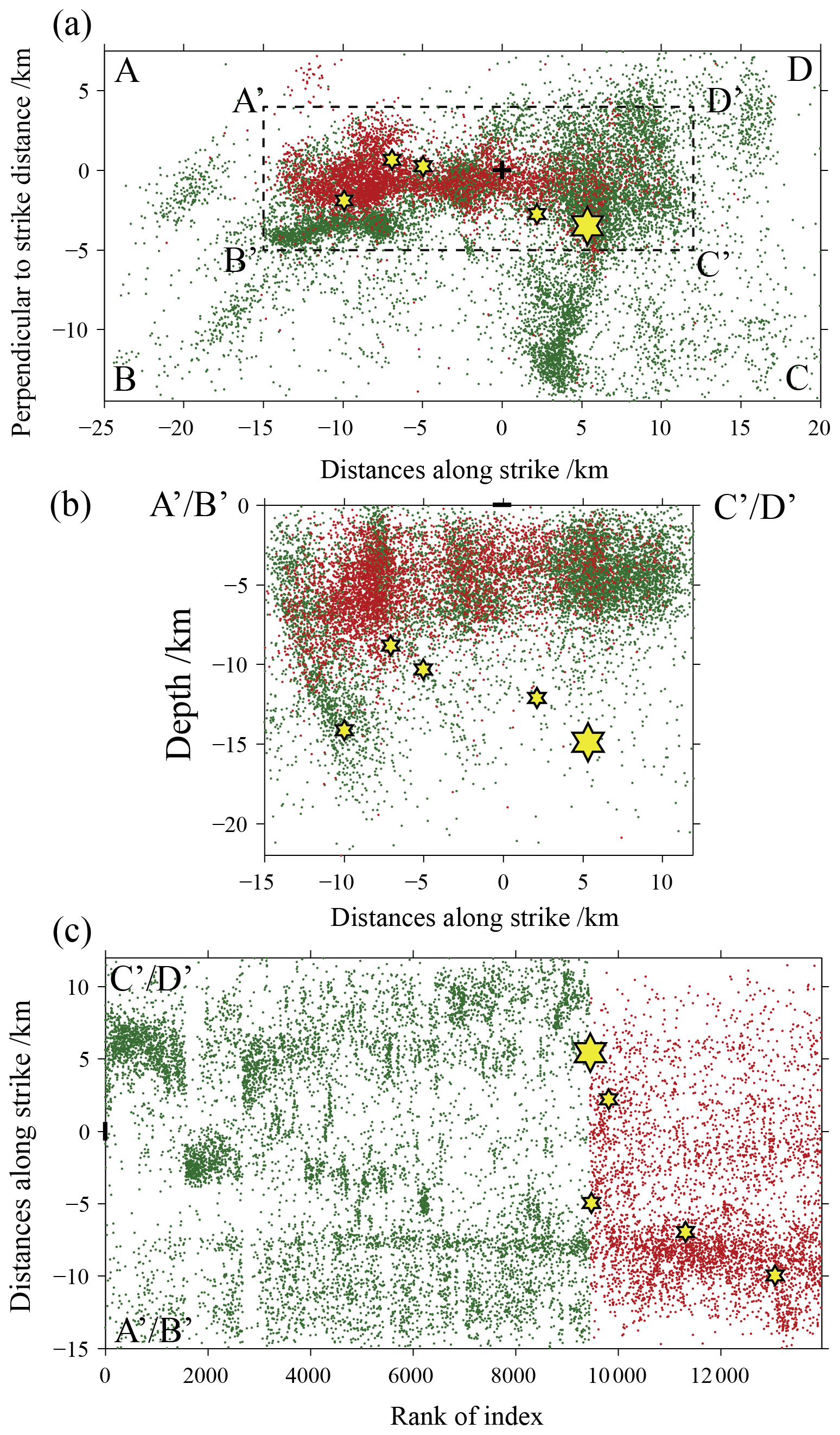
Figure 2Distribution of seismicity for b-value calculations. (a) Rotation of the coordinate system to the seismic distribution along the direction of the aftershock distribution; (b) projection of the earthquakes in the rectangular frame A′B′C′D′ on the depth profile; (c) the temporal and spatial distribution on the distance versus rank of index 2-D map of the earthquakes within the rectangular frame A′B′C′D′. The meaning of the symbols is the same as in Fig. 1.
According to the technical process of the data-driven approach described above, after Voronoi tessellation, calculation of the BIC values, and selection of the optimal models, the ensemble median (Q2) and ensemble median absolute deviation (MAD) of b values can be obtained. Figure 3 shows an example of calculating the parameters of the OK1993 model in terms of the frequency–magnitude distribution based on a data-driven approach. Figure 3a is the distribution of those BIC values corresponding to the number of effective cells NV, and the red dots are the selected best-100 models. Figure 3b shows an example of the best-100 models, that is, in the case of NV=20, the Voronoi tessellation in the rectangular study area ABCD and the distribution of b values obtained by its calculation. Figure 3c shows an example of the fitting result of the OK1993 model corresponding to a cell in Fig. 3b. The OK1993 model parameters obtained by the fitting are b=0.714, μ=0.376, and σ=0.247.
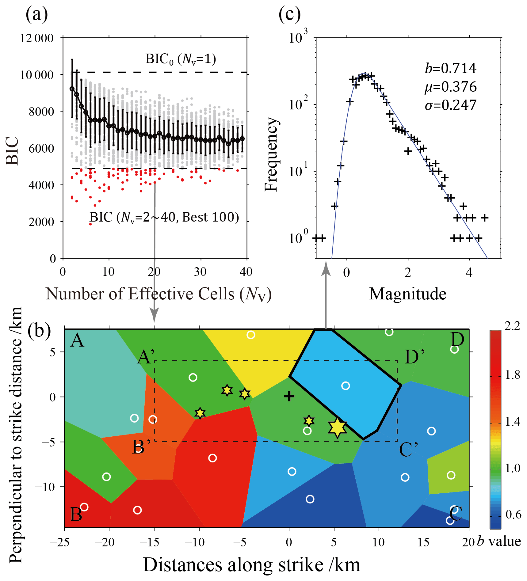
Figure 3An example of calculating the parameters of the OK1993 model in terms of the frequency–magnitude distribution based on a data-driven approach. (a) Distribution of BIC values versus the number of effective cells Nv in the Voronoi tessellation. The black dots and error bars are commensurate with the mean value and 1 standard deviation of BIC values under the corresponding Nv, respectively. The top horizontal dashed line marks the BIC values of the entire spatial region without mesh generation (BIC0, Nv=1). The red dots show the BIC values with the best-100 solutions selected, while the gray dots are the other BIC results according to Nv. (b) Example of Voronoi tessellation of Nv=20 and one of the best-100 models selected. The white circles are the positions of the Voronoi nodes, and the resulting partitions are color coded by their estimated b values (obtained from the β value in the OK1993 model). (c) Example of fitting result for the frequency–magnitude distribution (FMD) of the OK1993 model in the Voronoi cell indicated by a thick line in graph (b).
We calculated the distribution of the ensemble median b value in the rectangular region ABCD and the depth profile of the rectangular region A′B′C′D′. The results are shown in Fig. 4. Figure 4a and b are the result before the Changning MS=6.0 earthquake and the entire study period, respectively. The results show that the b values exhibit a strong heterogeneous spatial distribution in the rectangular region ABCD before the Changning MS=6.0 earthquake. Low b values are mainly distributed in the eastern half of the area, with its lowest value being b=0.732 and located near the epicenter of the mainshock. Low-b-value contours are mainly distributed in the NE–SW direction and are consistent with the direction of the Shuanghechang anticline and its associated faults passing through the main epicenter. In the western part of the rectangular region ABCD, high b values are distributed, with a largest value of b=2.200. This indicates that before the Changning MS=6.0 earthquake, the differential stress near the epicenter of the mainshock was high, but the spatial scale of this larger differential stress was much smaller than the scale of the aftershock spatial distribution. The spatial distribution of b values calculated using all seismic events (see Fig. 4b) shows that the area with low b values in the region ABCD is significantly enlarged, and the b values in the rectangular region A′B′C′D′ are almost less than 1.0 and further reduced to 0.698 near the epicenter of the mainshock. This phenomenon of a significant decrease in the b value of the aftershock sequence after the mainshock widely exists in many earthquake cases (El-Isaa and Eatonb, 2014; Gulia and Wiemer, 2019).
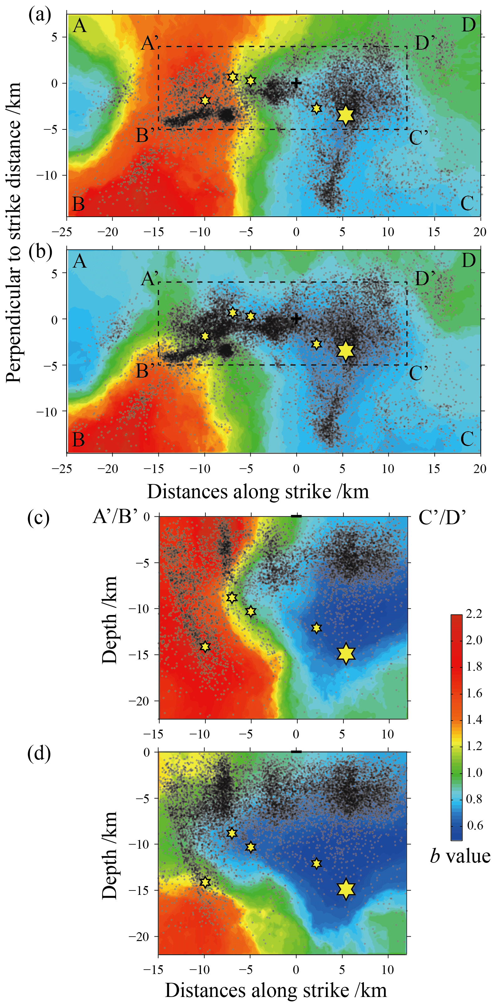
Figure 4The spatial distribution of the ensemble median b values of the best-100 solutions for Nv=2–Nv=40 in the Changning area. (a) The ensemble median b values before the Changning MS=6.0 earthquake is distributed on the horizontal plane after the rotation; (b) the ensemble median b values obtained by calculation of the whole earthquake including the aftershocks of the Changning MS=6.0 earthquake distributed on the horizontal plane after the rotation; (c) distribution of the ensemble median b values before the occurrence of the Changning MS=6.0 earthquake in the rectangular frame A′B′C′D′ on the depth profile; (d) distribution of ensemble median b values obtained by calculation of all earthquakes including aftershocks of the Changning MS=6.0 earthquake in the rectangular frame A′B′C′D′ on the depth profile. The black dots on each graph mark the seismic events used in the calculation.
Figure 4c and d show the distribution of the ensemble median b value on the depth profile of the rectangular area A′B′C′D′ and correspond to the results before the Changning MS=6.0 earthquake and all study periods, respectively. The calculation results after considering the depth information of the earthquake show that b values also have strong heterogeneity at different depths. Among them, in Fig. 4c, low b values are mainly distributed at a depth of 4–15 km, which contains the source of the Changning MS=6.0 earthquake and the 17 June 2019 MS=5.1 earthquake. The lowest b value is about 0.493, which is much smaller than the minimum value in Fig. 4a. In Fig. 4d, considering the occurrence of the Changning MS=6.0 earthquake sequence, the distribution area of low b values expands in the NW direction, and the lowest b value is about 0.501, which is close to that in Fig. 4c. Compared with the results obtained by ignoring the depth information of the earthquake in Fig. 4a and b, the results obtained by Fig. 4c and d reveal more significant heterogeneity of b values when we extend the investigation to different depths of the crust. Lower b values may indicate that there should be greater differential stress at the depth where the source area of the mainshock is located, and it is easily ignored by b-value calculations that usually do not consider the depth information of earthquake events.
Figure 5 shows the spatial distribution of the median absolute deviation (MAD) of b values by the data-driven approach according to Fig. 4. The ensemble MAD b value is smaller in most regions of Fig. 5a–d, especially in the rectangular region A′B′C′D′, which implies that these regions have relatively stable distribution and reliable ensemble median b values. As a comparison with Figs. 4 and 5, we also used the Changning MS=6.0 earthquake and aftershocks to calculate the ensemble median b values and MAD b values. For the corresponding results, please see Fig. S2.
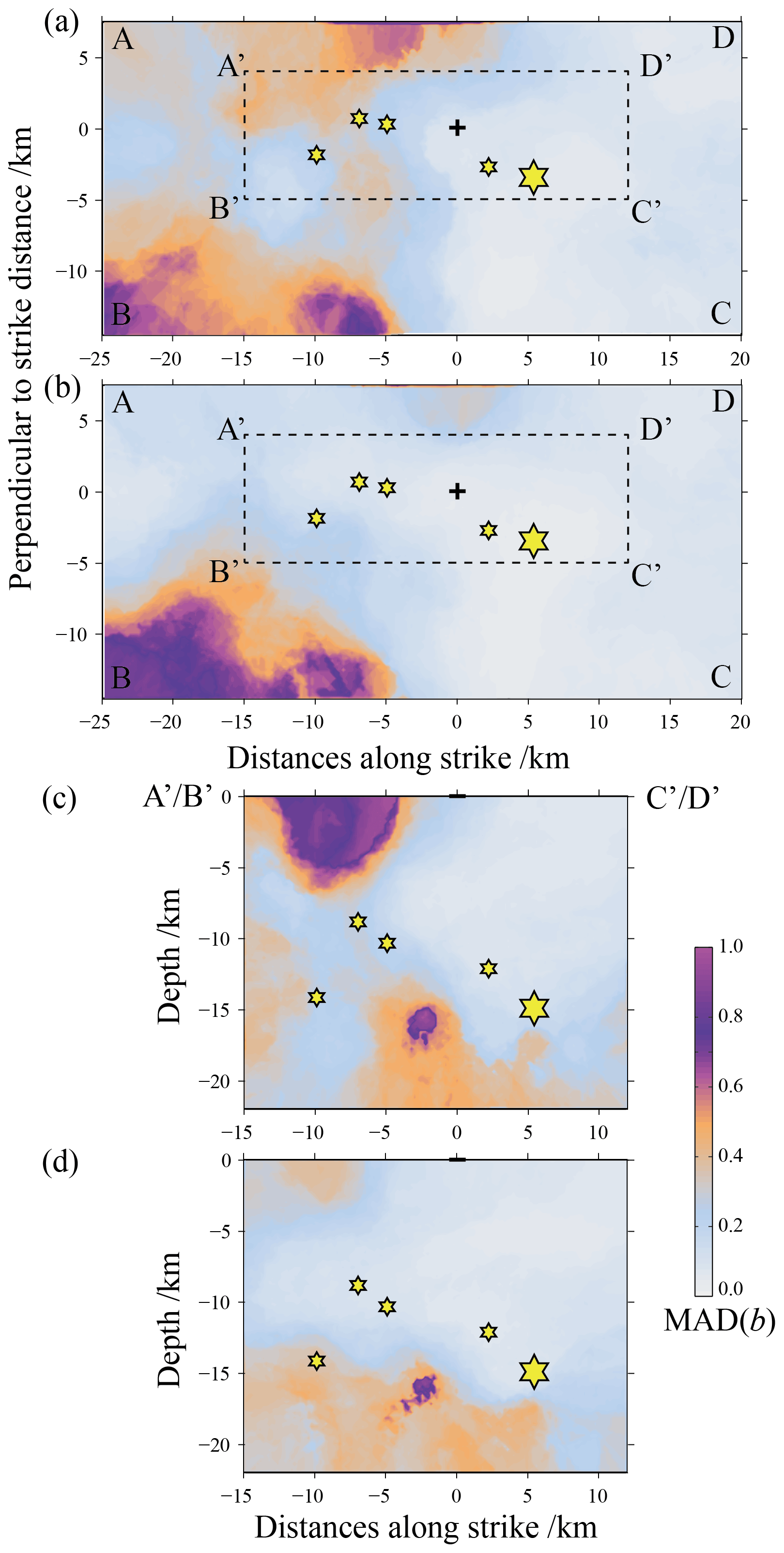
Figure 5The spatial distribution of the median absolute deviation (MAD) of the b values by the data-driven approach according to Fig. 4. (a) The ensemble MAD b values before the Changning MS=6.0 earthquake is distributed on the horizontal plane after the rotation; (b) the ensemble MAD b values obtained by calculation of the whole earthquake including the aftershocks of the Changning MS=6.0 earthquake distributed on the horizontal plane after the rotation; (c) distribution of the ensemble MAD b values before the occurrence of the Changning MS=6.0 earthquake in the rectangular frame A′B′C′D′ on the depth profile; (d) distribution of ensemble MAD b values obtained by calculation of all earthquakes including aftershocks of the Changning MS=6.0 earthquake in the rectangular frame A′B′C′D′ on the depth profile.
Considering that the b value usually changes over time before and after a strong earthquake, this paper not only examines the spatial distribution of b values in the surface and depth profiles but also discusses the spatiotemporal distribution of b values for earthquake events in the rectangular area A′B′C′D′ where the Changning MS=6.0 sequence is located. Due to the strong temporal and spatial inhomogeneity of seismic activity, especially clustering in time, there are great difficulties in obtaining a stable and reliable b value and clearly showing the temporal and spatial variation in the b value. In order to reduce this difficulty to a certain extent, here we use the index of earthquake occurrence instead of time; that is, the earthquake is projected on a pseudo-time axis of the index number of the occurrence time sequence. Using the same calculation method as in Figs. 4 and 5, the distributions of ensemble median b values and ensemble MAD b values on the distance–index map are obtained. The corresponding results are shown in Figs. 6 and 7. Considering the possible abrupt change in the regional stress field due to strong earthquakes such as the Changning MS=6.0 earthquake, we adopt two schemes to study the spatiotemporal distribution of b values. One is to study the seismicity before and after the mainshock as a whole, and the other is to study the seismicity before and after the mainshock as two independent periods. The calculation results under the two schemes are shown in Fig. 6a and b, respectively.

Figure 6Spatiotemporal distribution of the ensemble median b values of the best-100 solutions for Nv=2–40 in a 2-D space consisting of the distance along strike and rank of index. (a) The ensemble median b values obtained from all data before and after the Changning MS=6.0 earthquake; (b) the ensemble median b values obtained from the data before and after the Changning MS=6.0 earthquake considered separately. The vertical dotted line shows where the MS=6.0 earthquake occurred. The timescale is marked on the x axis (above the axis), including the time of whole years marked by long ticks and the half-year time marked by short ticks.
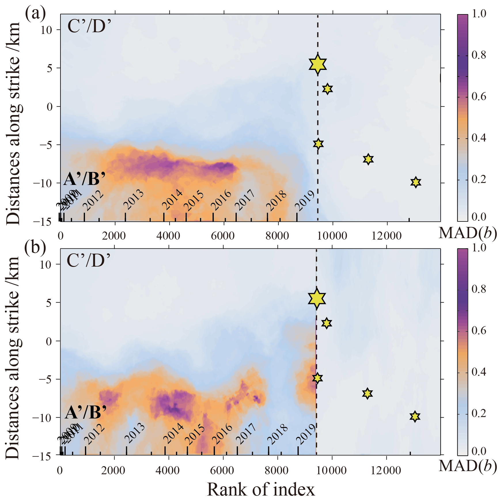
Figure 7Spatiotemporal distribution of the median absolute deviation (MAD) of the b values of the best-100 solutions for Nv=2–40 in a 2-D space consisting of distance along strike and rank of index. (a) The ensemble MAD b values obtained from all data before and after the Changning MS=6.0 earthquake; (b) the ensemble MAD b values obtained from the data before and after the Changning MS=6.0 earthquake considered separately. The vertical dotted line shows where the MS=6.0 earthquake occurred. The timescale is marked on the x axis (above the axis), including the time of whole years marked by long ticks and the half-year time marked by short ticks.
It can be seen in Fig. 6a that before the Changning MS=6.0 earthquake, in the segment between −5 and −10 km near the A′–B′ end and with a length of about 10 km (NW direction of the aftershocks in Fig. 1), there were relatively stable high b values, with the maximum value exceeding 2.0. In the segment between −5 and 12 km near the C′–D′ end and with a length of about 17 km (the SE direction of the aftershocks in Fig. 1, including the nucleation point of the mainshock), there were relatively stable low values before the Changning MS=6.0 earthquake, and the range of the low b values gradually narrowed and became concentrated towards the nucleation point of the mainshock. After the Changning MS=6.0 earthquake occurred, the b values in the entire spatial range from A′–B′ to C′–D′ decreased significantly. Among them, the b values in the 0–12 km segment where the nucleation point of the mainshock is located recovered rapidly, while the b values in the 0 to −15 km segment increased at a slower rate.
From the results before and after the Changning MS=6.0 earthquake shown in Fig. 6b, it can be seen that the occurrence of the mainshock has a greater impact on the continuity of time-variant b values. This means that the spatiotemporal evolution image of the b values given in Fig. 6a over the entire study period is not physically valid. Correspondingly, the decrease in pre-mainshock b values and the sudden expansion of the low b values may be a kind of artifact caused by the subsequent aftershocks brought into the calculation (Lei et al., 2019).
Compared with Fig. 6a, the results in Fig. 6b show that before the Changning MS=6.0 earthquake, the shortening and concentration changes for the low-b-value segment near the C′–D′ end and the expansion process of the high-b-value segment near the A′–B′ end are performed simultaneously. This implies that a significantly higher differential stress area is concentrated towards the nucleation point of the mainshock. Figure 7a and b show the distribution of ensemble MAD b values according to Fig. 6a and b, where higher ensemble MAD b values mainly appear in some areas with higher b values in Fig. 6a and b.
In the pattern of b-value spatial heterogeneity before strong earthquakes, the locations of rupture nucleation points, sliding distributions, and aftershock distributions of some strong earthquakes were observed to correspond to areas with lower b values, such as the Parkfield M=6.0 earthquake on 28 September 2004 (Wiemer and Wyss, 1997; Schorlemmer et al., 2004; Schorlemmer and Wiemer, 2005). However, the significant spatial heterogeneity of b values obtained from the studies of these earthquakes is suspected to be related to the subjective arbitrariness of the calculation rules (Kamer and Hiemer, 2015). The calculation results based on the data-driven method (Si and Jiang, 2019) in this paper show that significant spatial heterogeneity of b values can still be observed before the Changning MS=6.0 earthquake, especially on the depth profile of the fault. Moreover, according to the empirical relationship between the magnitude and rupture scale of Wells and Coppersmith (1994), the low-value spatial scale of b<0.75 in Fig. 4c is also close to the rupture length of about 10 km for the M=6.0 mainshock. This also means that it is still feasible to use the spatial heterogeneity of the b values to identify the locked asperities and determine the location of future strong earthquakes if more cases are verified.
There is still much controversy over the temporal variation pattern of b values in the source area before a strong earthquake. Although the decrease in b values prior to failure was found in laboratory fracturing experiments on relatively complete rock samples (e.g., Thompson et al., 2006; Lei, 2019) and in the case studies of strong earthquakes (Nanjo et al., 2012; Schurr et al., 2014; Bayrak et al., 2017; Huang et al., 2020), a large number of reported temporal variations in b values before actual strong earthquakes are still considered to have no statistically significant predictive power (Parsons, 2007). Some studies have found that the temporal variation in b values corresponding to asperities is synchronized with the loading rate and shear stress (Tormann et al., 2013). Schorlemmer et al. (2004) and Wiemer and Wyss (2002) studied some earthquake cases and concluded that the b value is quite stable over time and it is difficult to observe a significant change. The study of the relationship between acoustic emission events and stress in the stick-slip experiment shows that the complexity of the temporal variations in b values observed when sliding on rough fault planes may be due to fault-structure heterogeneity (Goebel et al., 2013). In this study of the Changning MS=6.0 earthquake, we did not simply examine the temporal variations in b values in a fixed spatial range but investigated the migration pattern of the b value in a 2-D spatiotemporal dimension. We found that as the time approaches the occurrence of the mainshock, the spatial range of the low b values gradually shrinks and focuses on the vicinity of the rupture nucleation point, and the b values do not decrease significantly. Under the assumption that the fault-structural heterogeneity will not change in the short term and based on previous understandings of the correlation between high b values and fluid-induced seismicity, the migration pattern in this paper may be explained by the erosion of fluid in the high-differential-stress area where the nucleation point is located.
For the spatiotemporal heterogeneity of the b value of the aftershocks of the 2019 Changning MS=6.0 earthquake, we noticed that the aftershocks expanded spatially to areas with high pre-mainshock b values in the northwest direction, and the length of the aftershock area was significantly longer than the rupture scale of the earthquake (see Fig. 6b). Since the aftershocks do not exhibit relatively slow spatiotemporal migration behavior, the physical mechanism that drives the aftershocks of this earthquake cannot be explained by either the traditional stress corrosion model (Das and Scholz, 1981) or the frictional afterslip model (Perfettini et al., 2018; Koper et al., 2018). Some views suggest that aftershock activity in high-b-value regions may be related to the reactivation of highly fractured fault zones, the redistribution of stress fields, and the role of fluids trapped in microfractures (Aktar et al., 2004). Long et al. (2020), imaging the velocity structure of the area where the Changning MS=6.0 earthquake was located, showed that there is an obvious S-wave low-velocity anomaly at the depth of 3 to 8 km in the northwestern segment of the aftershock. In this paper, this S-wave low-velocity anomaly region also corresponds to the distribution of high b values, which may be related to fluid intrusion. Therefore, we deduce that the abundant aftershocks produced by this mainshock and the active area that exceeds the rupture scale of the mainshock are more likely to be caused by the mainshock which triggered a series of complex structural aftershocks northwest of the nucleation point. The dynamic expansion of the region of high pre-mainshock b values to the nucleation point also creates conditions for the triggering of a large number of aftershocks that are widespread spatially.
In addition, b values of the aftershocks first dropped rapidly to about 0.5, then gradually recovered, and returned to the pre-seismic level after the fourth aftershock of magnitude 5 (excluding high-b-value areas). The phenomenon that the b values of the aftershock sequence decrease immediately after the mainshock and then rapidly recover has been observed in many earthquake cases (El-Isaa and Eatonb, 2014; Tormann et al., 2015). Unlike most aftershock sequences, where the b value generally increases by 20 % after the mainshock, this sudden decrease in the b value is considered to be related to the occurrence of subsequent strong aftershocks or larger earthquakes (Gulia and Wiemer, 2019). In the aftershock sequence of the Changning MS=6.0 earthquake, the rapidly decreasing b value of the aftershocks was accompanied by four strong aftershocks with magnitudes greater than 5.0, which is consistent with the phenomenon revealed by previous studies. This may also support the idea of discrimination between foreshocks and aftershocks by real-time monitoring of the b value in aftershock sequences (Gulia and Wiemer, 2019). However, it needs to be pointed out that similarly to the problem of sudden changes in the spatiotemporal distribution of b values before and after the mainshock, it cannot be ruled out that four strong aftershocks with M>5 will affect the continuity of the b values to a certain extent.
To reveal whether there is spatiotemporal heterogeneity of b values before and after the 2019 Changning MS=6.0 earthquake and to overcome the subjectivity of the choice of data used for calculation, we applied the OK1993 model of magnitude–frequency distribution according to the data-driven idea to calculate b values. We also investigated the distribution characteristics of b values in three different ways: horizontal surface distribution, depth profile distribution, and the distance–rank of index map. The main conclusions are as follows:
-
The b values before and after the Changning MS=6.0 earthquake showed strong spatiotemporal heterogeneity in the horizontal surface distribution, in the depth profile distribution, and on the distance–rank of index map. Among them, before the Changning MS=6.0 earthquake, there were obvious low-b-value distributions near the epicenter of the mainshock and within the depth range of 3 to 12 km. The correlation shows that there may be significantly higher differential stress in the source area before the Changning MS=6.0 earthquake. The northwestern segment of the aftershocks has a b-value distribution that is distinctly high, which coincides with the S-wave low-velocity anomaly region shown by the velocity structure imaging.
-
The b-value spatiotemporal distribution results show that before the Changning MS=6.0 earthquake, the high-b-value region of the NW segment spread by aftershocks gradually expanded and approached the nucleation point as the time approached the failure time of the mainshock. This may be related to the fluid intrusion in the rock. A large number of aftershocks were produced, and the area where the aftershocks were spread was significantly larger than the rupture scale of the mainshock. The mainshock may have triggered seismicity in the NW direction where the fluid intrudes.
-
The b values of the aftershocks of the Changning MS=6.0 earthquake decreased rapidly and gradually recovered after the mainshock, indicating a higher differential stress level in the aftershock area. The time variation in low b values is synchronized with the occurrence of strong aftershocks with M≥5.0, showing the application potential that can be used to distinguish between foreshocks and aftershocks.
-
Although the distribution characteristics of b values before and after the Changning MS=6.0 earthquake were qualitatively consistent when they were studied in different space-time dimensions, there were significant differences in specific b values. For example, the minimum b value of the Changning MS=6.0 earthquake in the depth profile distribution is about 0.493, but it is about 0.732 when the seismic depth information is ignored and the value is only calculated on the surface. This inconsistency needs special attention when studying the spatiotemporal heterogeneity of b values.
The MATLAB code for the data-driven method used to compute the b values can be obtained by contacting Changsheng Jiang (jiangcs@cea-igp.ac.cn).
The relocated earthquake catalog can be obtained by contacting Changsheng Jiang (jiangcs@cea-igp.ac.cn).
The supplement related to this article is available online at: https://doi.org/10.5194/nhess-21-2233-2021-supplement.
CJ, LH and FL contributed to the conceptualization. CJ prepared the manuscript with contributions from all authors. CS and LH wrote software for data processing. GL, FY, JB, and ZS contributed to the revised manuscript version.
The authors declare that they have no conflict of interest.
Publisher's note: Copernicus Publications remains neutral with regard to jurisdictional claims in published maps and institutional affiliations.
The earthquake catalog used in this paper was provided by the Sichuan Earthquake Agency. The Multi-Parametric Toolbox 3.0 (https://www.mpt3.org/Main/HomePage, last access: June 2018) was used for the analysis of parametric optimization and computational geometry. We thank the editor and two anonymous reviewers for their very helpful comments and suggestions.
This research has been supported by the program of the China Seismic Experimental Site (grant no. 2019CSES0106); the program of Basic Resources Investigation of Science and Technology (grant no. 2018FY100504); the National Natural Science Foundation of China (grant no. U2039204); and the Special Fund of the Institute of Geophysics, China Earthquake Administration (grant no. DQJB20X11).
This paper was edited by Filippos Vallianatos and reviewed by two anonymous referees.
Aktar, M., Özalaybey, S., Ergin, M., Karabulut, H., Bouin, M.-P., Tapırdamaz, C., Biçmen, F., Yörük, A., and Bouchon, M.: Spatial variation of aftershock activity across the rupture zone of the 17 August 1999 Izmit earthquake, Turkey, Tectonophysics, 391, 325–334, https://doi.org/10.1016/j.tecto.2004.07.020, 2004.
Amelung, F. and King, G.: Earthquake scaling laws for creeping and non-creeping faults, Geophys. Res. Lett., 24, 507–510, https://doi.org/10.1029/97GL00287, 1997.
Amorèse, D., Grasso, J.-R., and Rydelek, P.: On varying b-values with depth, results from computer-intensive tests for Southern California, Geophys. J. Int., 180, 347–360, https://doi.org/10.1111/j.1365-246X.2009.04414.x, 2010.
Bayrak, E., Yılmaz, S., and Bayrak, Y.: Temporal and spatial variations of Gutenberg–Richter parameter and fractal dimension in Western Anatolia, Turkey, J. Asian Earth Sci., 138, 1–11, https://doi.org/10.1016/j.jseaes.2017.01.031, 2017.
Das, S. and Scholz, C.: Theory of time-dependent rupture in the Earth, J. Geophys. Res., 86, 6039–6051, https://doi.org/10.1029/JB086iB07p06039, 1981.
Del Pezzo, E., Bianco, F., and Saccorotti, G.: Duration magnitude uncertainty due to seismic noise, Inferences on the temporal pattern of GR b-value at Mt. Vesuvius, Italy, Bull. Seismol. Soc. Am., 93, 1847–1853, https://doi.org/10.1785/0120020222, 2003.
El-Isaa, Z. H. and Eatonb, D. W.: Spatiotemporal variations in the b-value of earthquake magnitude–frequency distributions, Classification and causes, Tectonophysics, 615–616, 1–11, https://doi.org/10.1016/j.tecto.2013.12.001, 2014.
Goebel, T. H. W., Schorlemmer, D., Becker, T., Dresen, G., and Sammis, C.: Acoustic emissions document stress changes over many seismic cycles in stick-slip experiments, Geophys. Res. Lett., 40, 2049–2054, https://doi.org/10.1002/grl.50507, 2013.
Gulia, L. and Wiemer, S.: Real-time discrimination of earthquake foreshocks and aftershocks, Nature, 574, 193–199, https://doi.org/10.1038/s41586-019-1606-4, 2019.
Gulia, L., Wiemer, S., and Schorlemmer, D.: Asperity-based earthquake likelihood models for Italy, Ann. Geophys., 533, 63–75, https://doi.org/10.4401/ag-4843, 2010.
Hainzl, S. and Fischer, T.: Indications for a successively triggered rupture growth underlying the 2000 earthquake swarm in Vogtland/NW Bohemia, J. Geophys. Res., 107, ESE 5-1–ESE 5-9, https://doi.org/10.1029/2002JB001865, 2002.
He, D. F., Lu, R. Q., Huang, H. Y., Wang, X. S., Jiang, H., and Zhang, W. K.: Tectonic and geological background of the earthquake hazards in Changning shale gas development zone, Sichuan Basin, SW China, Petrol. Explor. Dev., 46, 1051–1064, https://doi.org/10.1016/S1876-3804(19)60262-4, 2019.
Huang, H., Meng, L. S., Bürgmann, R., Wang, W., and Wang, K.: Spatio-temporal foreshock evolution of the 2019 M6.4 and M7.1 Ridgecrest, California earthquakes, Earth Planet. Sc. Lett., 551, 116582, https://doi.org/10.1016/j.epsl.2020.116582, 2020.
Hutton, K., Woessner, J., and Hauksson, E.: Earthquake monitoring in southern California for seventy-seven years (1932–2008), Bull. Seismol. Soc. Am., 100, 423–446, https://doi.org/10.1785/0120090130, 2010.
Kagan, Y. Y.: Universality of the seismic moment-frequency relation, Pure Appl. Geophys., 155, 537–573, https://doi.org/10.1007/s000240050277, 1999.
Kamer, Y. and Hiemer, S.: Data-driven spatial b value estimation with applications to California seismicity, To b or not to b, J. Geophys. Res., 120, 5191–5214, https://doi.org/10.1002/2014JB011510, 2015.
Koper, K. D., Pankow, K. L., Pechmann, J. C., Hale, J. M., Burlacu, R., Yeck, W. L., Benz, H. M., Herrmann, R. B., Trugman, D. T., and Shearer, P. M.: Afterslip enhanced aftershock activity during the 2017 earthquake sequence near Sulphur Peak, Idaho, Geophys. Res. Lett., 45, 5352–5361, https://doi.org/10.1029/2018GL078196, 2018.
Lei, X., Wang, Z., and Su, J.: Possible link between long-term and short-term water injections and earthquakes in salt mine and shale gas site in Changning, south Sichuan Basin, China, Earth Planet. Phys., 36, 510–525, https://doi.org/10.26464/epp2019052, 2019.
Lei, X. L.: Evolution of b-value and fractal dimension of acoustic emission events during shear rupture of an immature fault in Granite, Appl. Sci., 9, 2498, https://doi.org/10.3390/app9122498, 2019.
Lei, X. L. and Satoh, T.: Indicators of critical point behavior prior to rock failure inferred from pre-failure damage, Tectonophysics, 431, 97–111, https://doi.org/10.1016/j.tecto.2006.04.023, 2007.
Long, F., Zhang, Z., Qi, Y., Liang, M., Ruan, X., Wu, W., Jiang, G., and Zhou, L.: Three dimensional velocity structure and accurate earthquake location in Changning–Gongxian area of southeast Sichuan, Earth Planet. Phys., 42, 1–15, https://doi.org/10.26464/epp2020022, 2020.
Mori, J. and Abercrombie, R. E.: Depth dependence of earthquake frequency-magnitude distributions in California, Implications for rupture initiation, J. Geophys. Res., 102, 15081–15090, https://doi.org/10.1029/97JB01356, 1997.
Murru, M., Console, R., Falcone, G., Montuori, C., and Sgroi, T.: Spatial mapping of the b value at Mount Etna, Italy, using earthquake data recorded from 1999 to 2005, J. Geophys. Res., 112, B12303, https://doi.org/10.1029/2006JB004791, 2007.
Nandan, S., Ouillon, G., Wiemer, S., and Sornette, D.: Objective estimation of spatially variable parameters of epidemic type aftershock sequence model, Application to California, J. Geophys. Res., 122, 5118–5143, https://doi.org/10.1002/2016JB013266, 2017.
Nanjo, K. Z., Hirata, N., Obara, K., and Kasahara, K.: Decade-scale decrease in b value prior to the M9-class 2011 Tohoku and 2004 Sumatra quakes, Geophys. Res. Lett., 39, L20304, https://doi.org/10.1029/2012GL052997, 2012.
Ogata, Y.: Significant improvements of the space-time ETAS model for forecasting of accurate baseline seismicity, Earth Planets Space, 63, 217–229, https://doi.org/10.5047/eps.2010.09.00, 2011.
Ogata, Y. and Katsura, K.: Analysis of temporal and spatial heterogeneity of magnitude frequency distribution inferred from earthquake catalogues, Geophys. J. Int., 113, 727–738, https://doi.org/10.1111/j.1365-246X.1993.tb04663.x, 1993.
Parsons, T.: Forecast experiment: Do temporal and spatial b value variations along the Calaveras fault portend M≥4.0 earthquakes?, J. Geophys. Res., 112, B03308, https://doi.org/10.1029/2006JB004632, 2007.
Perfettini, H., Frank, W., Marsan, D., and Bouchon, M.: A model of aftershock migration driven by afterslip, Geophys. Res. Lett., 455, 2283–2293, https://doi.org/10.1002/2017GL076287, 2018.
Rubner, Y., Tomasi, C., and Guibas, L. J.: The earth mover's distance as a metric for image retrieval, Int. J. Comput. Vis., 40, 99–121, https://doi.org/10.1023/A:1026543900054, 2000.
Sambridge, M., Bodin, T., Gallagher, K., and Tkalčić, H.: Transdimensional inference in the geosciences, Philos. T. Roy. Soc. A, 371, 20110547, https://doi.org/10.1098/rsta.2011.0547, 2013.
Scholz, C. H.: The frequency-magnitude relation of microfracturing in rock and its relation to earthquakes, Bull. Seismol. Soc. Am., 581, 399–415, 1968.
Schorlemmer, D. and Wiemer, S.: Microseismicity data forecast rupture area, Nature, 434, 1086, https://doi.org/10.1038/4341086a, 2005.
Schorlemmer, D., Wiemer, S., and Wyss, M.: Earthquake statistics at Parkfield, 1. Stationarity of b values, J. Geophys. Res., 109, B12307, https://doi.org/10.1029/2004JB003234, 2004.
Schurr, B., Asch, G., Hainzl, S., Bedford, J., Hoechner, A., Palo, M., Wang, R., Moreno, M., Bartsch, M., Zhang, Y., Oncken, O., Tilmann, F., Dahm, T., Victor, P., Barrientos, S., and Vilotte, J.: Gradual unlocking of plate boundary controlled initiation of the 2014 Iquique earthquake, Nature, 512, 299–302, https://doi.org/10.1038/nature13681, 2014.
Si, Z. Y. and Jiang, C. S.: Research on parameter calculation for then Ogata–Katsura 1993 model in terms of the frequency–magnitude distribution based on a data-driven approach, Seismol. Res. Lett., 90, 1318–1329, https://doi.org/10.1785/0220180372, 2019.
Stirling, M. W., Wesnousky, S. G., and Shimazaki, K.: Fault trace complexity, cumulative slip, and the shape of the magnitude-frequency distribution for strike-slip faults, A global survey, Geophys. J. Int., 124, 833–868, https://doi.org/10.1111/j.1365-246X.1996.tb05641.x, 1996.
Svec, L., Burden, S., and Dilley, A.: Applying Voronoi diagrams to the redistricting problem, UMAP J., 28, 313–329, 2007.
Thompson, B. D., Young, R. P., and Lockner, D. A.: Fracture in Westerly granite under AE feedback and constant strain rate loading, nucleation, quasi-static propagation, and the transition to unstable fracture propagation, Pure Appl. Geophys., 163, 995–1019, https://doi.org/10.1007/s00024-006-0054-x, 2006.
Toda, S., Stein, R. S., Reasenberg, P. A., Dieterich, J. H., and Yoshida, A.: Stress transferred by the 1995 Mw=6.9 Kobe, Japan, shock, Effect on aftershocks and future earthquake probabilities, J. Geophys. Res., 103, 24543–24565, https://doi.org/10.1029/98JB00765, 1998.
Tormann, T., Wiemer, S., Metzger, S., Michael, A., and Hardebeck, J. L.: Size distribution of Parkfield's microearthquakes reflects changes in surface creep rate, Geophys. J. Int., 193, 1474–1478, https://doi.org/10.1093/gji/ggt093, 2013.
Tormann, T., Enescu, B., Woessner, J., and Wiemer, S.: Randomness of megathrust earthquakes implied by rapid stress recovery after the Japan earthquake, Nat. Geosci., 8, 152–158, https://doi.org/10.1038/ngeo2343, 2015.
Urbancic, T. I., Trifu, C. I., Long, J. M., and Young, R. P.: Space-time correlations of b values with stress release, Pure Appl. Geophys., 139, 449–462, https://doi.org/10.1007/BF00879946, 1992.
Waldhauser, F. and Ellsworth, W. L.: A double-difference earthquake location algorithm, method and application to the Northern Hayward fault, California, Bull. Seismol. Soc. Am., 90, 1353–1368, https://doi.org/10.1785/0120000006, 2000.
Wells, D. L. and Coppersmith, K. J.: New empirical relationships among magnitude, rupture length, rupture width, rupture area, and surface displacement, Bull. Seismol. Soc. Am., 844, 974–1002, 1994.
Wiemer, S. and Schorlemmer, D.: ALM, An asperity-based likelihood model for California, Seismol. Res. Lett., 781, 134–140, https://doi.org/10.1785/gssrl.78.1.134, 2007.
Wiemer, S. and Wyss, M.: Mapping the frequency-magnitude distribution in asperities, an improved technique to calculate recurrence times?, J. Geophys. Res., 102, 15115–15128, https://doi.org/10.1029/97JB00726, 1997.
Wiemer, S. and Wyss, M.: Mapping spatial variability of the frequency-magnitude distribution of earthquakes, Adv. Geophys., 45, 259–302, https://doi.org/10.1016/S0065-2687(02)80007-3, 2002.
Woessner, J. and Wiemer, S.: Assessing the quality of earthquake catalogues, Estimating the magnitude of completeness and its uncertainty, Bull. Seismol. Soc. Am., 95, 684–698, https://doi.org/10.1785/0120040007, 2005.
Wyss, M.: Towards a physical understanding of the earthquake frequency distribution, Geophys. J. Roy. Astron. Soc., 31, 341–359, https://doi.org/10.1111/j.1365-246X.1973.tb06506.x, 1973.
Wyss, M., Schorlemmer, D., and Wiemer, S.: Mapping asperities by minima of local recurrence time, San Jacinto-Elsinore fault zones, J. Geophys. Res., 105, 7829–7844, https://doi.org/10.1029/1999JB900347, 2000.
Xie, J., Ni, S., and Zeng, X.: 1 D shear wave velocity structure of the shallow upper crust in central Sichuan Basin, Earthq. Res. Sichuan, 143, 20–24, https://doi.org/10.3969/j.issn.1001-8115.2012.02.004, 2012.
Yi, G. X., Long, F., Liang, M. J., Zhao, M., Wang, S. W., Gong, Y., Qiao, H. Z., and Su, J. R.: Focal mechanism solutions and seismogenic structure of the 17 June 2019 MS6.0 Sichuan Changning earthquake sequence, Chinese J. Geophys., 62, 3432–3447, https://doi.org/10.6038/cjg2019N0297, 2019.
- Abstract
- Introduction
- Method
- Study region and data used
- Spatial distributions of b values in surface and depth profiles
- Spatiotemporal heterogeneity of b values
- Discussion
- Conclusions
- Code availability
- Data availability
- Author contributions
- Competing interests
- Disclaimer
- Acknowledgements
- Financial support
- Review statement
- References
- Supplement