Assimilation of Himawari-8 imager radiance data with the WRF-3DVAR system for the prediction of Typhoon Soudelor

Himawari-8 is a next-generation geostationary meteorological satellite launched by the Japan Meteorological Agency. It carries the Advanced Himawari Imager (AHI) on board, which can continuously monitor high-impact weather events with high frequency in space and time. The assimilation of AHI radiance data was implemented with the three-dimensional variational data assimilation system (3DVAR) of the Weather Research and Forecasting Model for the analysis and prediction of Typhoon Soudelor (2015) in the Pacific typhoon season. The effective assimilation of AHI radiance data in improving the forecast of the tropical cyclone during its rapid intensification has been realized. The results show that, after assimilating the AHI radiance data under clear-sky conditions, the typhoon position in the background field of the model was effectively corrected compared with the control experiment without AHI radiance data assimilation. It is found that the assimilation of AHI radiance data is able to improve the analyses of the water vapor and wind in a typhoon's inner-core region. The analyses and forecasts of the minimum sea level pressure, the maximum surface wind, and the track of the typhoon are further improved.

1 Introduction

In recent years, although researchers have made great progress in the field of numerical weather prediction (NWP), huge challenges are encountered in the accurate forecasting of tropical cyclones (TCs) with rapid intensifications (DeMaria et al., 2014). The predictability of these TCs is limited because it entails complex multi-scale dynamic interactions (Minamide and Zhang, 2018). These interactions include environmental airflows, TC vortex interactions, atmosphere–ocean interactions, and the effects of mesoscale and micro-convective scale, together with the microphysics and atmospheric radiation. In order to attain a better initial condition and improve the accuracy of the forecast, data assimilation (DA) seeks to fully utilize the observations. The life span of most TCs is over the ocean, where conventional observations are relatively insufficient compared to the land. Therefore, by analyzing observed data from satellites and planes over the ocean, it is crucial to adopt effective DA methods to improve the analysis and forecast of TCs.

With the rapid development of atmospheric radiative transfer models, many numerical weather prediction centers have adopted variational DA methods to assimilate a variety of radiance data from different satellite observation instruments (Bauer et al., 2011; Buehner et al., 2016; Derber and Wu, 1998; Hilton et al., 2009; Kazumori, 2014; McNally et al., 2006; Prunet et al., 2000). These data can take up 90 % of all data used in global DA system and can improve the accuracy of the numerical model results strikingly (Bauer et al., 2010). Some researches have demonstrated that, in global models, satellite radiance DA makes more of a contribution to improving the accuracy of the numerical model results than conventional observation DA does (Zapotocny et al., 2007; Yan et al., 2010; Geer et al., 2017).

Generally speaking, radiance data are derived from microwave and infrared detecting instruments, which are from polar-orbit satellites and geostationary satellites, respectively. Polar-orbit satellites cover the sphere of all the Earth and are therefore suitable for global NWP models (Jung et al., 2008). Furthermore, they have finer resolutions compared to geostationary satellites (Li and Zou, 2017; Shen and Min, 2015; Xu et al., 2013). However, it is highlighted that they are not able to generate continuous observations for a fixed regional area and so may miss rapidly intensified TCs or storms. However, because geostationary satellites rotate with the Earth, although their resolutions are lower than those of polar-orbit satellites, they can capture the formation and development of mesoscale convective systems by continuous monitoring (Montmerle et al., 2007; Stengel et al., 2009; Zou et al., 2011).

Geostationary satellites are able to continuously detect a region at a higher frequency, thus observing TCs over the vast ocean effectively. As the first new-generational geostationary satellite, Himawari-8 plays a pioneering role for the geosynchronous imagers to be launched in the USA, China, Korea, and Europe. It has an advanced imager called Advanced Himawari Imager (AHI) with 16 visible and infrared bands, including 3 moisture channels, which can conduct a full-disk scan every 10 min. Meanwhile, it can also acquire regional scanning images, and that is to say it can scan Japan and the target areas every 2.5 min. Compared to the early geosynchronous imagers, AHI has more spectrum bands and thus can monitor the state of the atmosphere with a higher frequency.

In recent years, some experts and scholars have carried out some studies on the data assimilation of geostationary satellite observations. Firstly, utilizing Gridpoint Statistical Interpolation (GSI) from the National Centers for Environmental Prediction (NCEP), Zou et al. (2011) conducted direct assimilation on imagers' data from GOES-11 and GOES-12 to estimate their potential influences on quantitative precipitation forecasts (QPFs) of coastal regions in the eastern part of the USA. They found that assimilating radiance data from GOES's imager has a remarkable improvement on 6–12 h QPFs near the northern coast of the Gulf of Mexico. Their work was continued by Qin et al. (2013), who put thinned radiance data into the GSI system to conduct a comprehensive investigation on the issue of combined assimilation of GOES Imager data together with the Advance Microwave Sounding Unit-A (AMSU-A), Advance Microwave Sounding Unit-B (AMSU-B), Atmospheric Infrared Sounder (AIRS), Microwave Humidity Sounder (MHS), High Resolution Infrared Radiation Sounder (HIRS), and GOES Sounder (GSN). The results showed the effect of single assimilation of AHI radiance data is better than combined assimilation in term of precipitation forecast. Zou et al. (2015) adopted the GSI system to assimilate radiance data from four infrared channels on GOES-13 and GOES-15 and set up two experiments for comparison. A symmetric vortex was used for initialization in the first experiment, and an asymmetric counterpart for the other experiment. Results showed that direct assimilation of GOES-13's and GOES-15's radiance data could yield positive effects on the track and intensity forecasts of Hurricane Debbie. Given that the Himawari-8 instrument is new, there are few studies on the DA of Himawari-8 data. Ma et al. (2017) used four-dimensional ensemble variational (4DEnVar) DA in NCEP's GSI system to assimilate radiance of three moisture channels of AHI radiance data under clear-sky conditions, and then NCEP's Global Forecast System (GFS) was utilized to estimate the impacts of AHI radiance data assimilation on weather forecast. They found it had a positive impact on the forecast of global vapor at high levels of the troposphere. Wang et al. (2018) investigated the impact of assimilating three water vapor channels under clear-sky conditions on the analysis and forecast of a rainstorm in northern China with the three-dimensional variational data assimilation system (3DVAR) method. They pointed out that the assimilation of AHI radiance data could improve the wind and vapor fields and the accuracy of rainfall forecast in the first 6 h lead time.

Although previous researches have made several advancements in satellite data assimilation and application, it is still a challenge to make more effective use of the new generation of geostationary satellite imager data with high spatial and temporal resolution. In most of the previous studies, researches usually use a 6 h or even longer time interval with a coarse spatial resolution. Therefore, the rapid updating assimilation techniques of the geostationary satellite radiance data have not been well carried out at convective scale. This study intends to build a data assimilation system aiming at AHI radiance data based on the new-generation mesoscale Weather Research and Forecasting (WRF) model. The case of Typhoon Soudelor is studied by performing numerical simulation to address the impacts of convective DA on the improvement of the initial conditions of TC and the enhancement of track and intensity forecasts. Our study focuses mainly on assimilating the three water vapor channels (6.2, 6.9, and 7.3 µm) since they are very sensitive to the humidity in the middle and upper troposphere and have a certain effect on the lower troposphere. Thus, a large amount of effective atmospheric information can be provided for AHI radiance data assimilation in the troposphere. The weighting functions for the three channels are provided in Fig. 1.

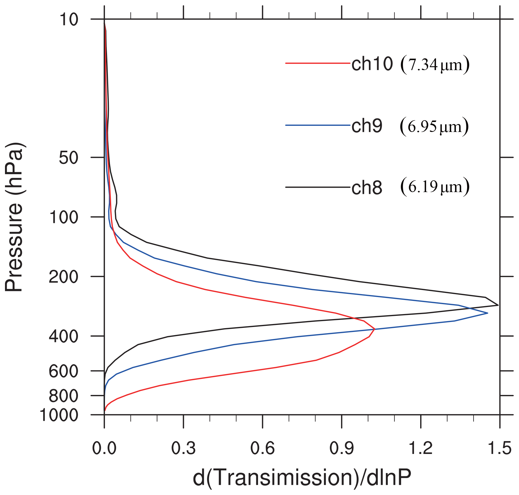
Figure 1 Weighting functions of the Himawari-8 Advanced Himawari Imager's three water vapor channels for channels 8–10.

Section 2 describes the observations and the data assimilation system. Introductions to the typhoon case and the experimental setup are provided in Sect. 3. The detailed results in terms of the analyses and the forecasts are illustrated in Sect. 4 before conclusions are summarized in Sect. 5.

2 Observational data and DA system

2.1 An introduction to Himawari-8 AHI radiance data

Himawari-8 satellite was launched by JMA to a geosynchronous orbit on 17 October 2014 and began its operational use on 7 July 2015 (Bessho et al., 2016). It is located between the Equator and 140.7^∘ E; thus the Earth is observed between 60^∘ N and 60^∘ S meridionally and between 80^∘ E and 160^∘ W zonally. Compared to its previous generation, Himawari-7, its detective ability has been significantly improved with the instrument AHI on Himawari-8. Furthermore, its device is comparable to imagers on the American GOES-R satellite (Goodman et al., 2012; Schmit et al., 2005, 2008, 2017). AHI is able to provide a full-disk image every 10 min and complete a scan over Japan every 2.5 min. AHI conducts continuous scan and detection on a moving targeted typhoon. It has 16 channels covering visible, near-infrared, and infrared spectral bands with a resolution of 0.5, 1, and 2 km, respectively. Channels 8 to 10 (6.2, 6.9, and 7.3 µm) are water vapor bands that are sensitive to the humidity in the middle and upper troposphere (Di et al., 2016). Other channels (channels 11, 12, and 16: 8.6, 9.6, and 13.3 µm, respectively) are monitoring other fields – such as the thin ice clouds, volcanic SO₂ gas, the ozone, or CO₂ – or the atmospheric window channels (13–15: 10.4, 11.2, and 12.4 µm, respectively) function as monitors for ice crystal/water, low water vapor, volcanic ash, sea surface temperature, and other phenomena (Bessho et al., 2016).

2.2 WRFDA system and AHI radiance data

The WRFDA system is designed by the National Center for Atmospheric Research, and it contains 3DVAR, 4DVAR, and hybrid parts. This research is based on the 3DVAR method. An interface that is suitable for AHI DA is built in the WRFDA system. Currently, WRFDA is able to assimilate many conventional and unconventional observations. In terms of satellite radiance data, this system is compatible with the Radiative Transfer for the Television Infrared Observational Satellite Operational Vertical Sounder (RTTOV) and Community Radiative Transfer Model (CRTM; Liu and Weng, 2006) as observation operators. In this study, CRTM is utilized as the observation operator to simulate and compute AHI radiance data. Estimating the systematic bias and random error of the observations caused by the errors of numerical models and instruments is key to directly assimilating the satellite radiance data. Apart from eliminating cloud pixels, other procedures are implemented inside the data assimilation framework for quality control as follows. (1) When reading the data, remove the observed outliers with values below 50 K or above 550 K. (2) Only the marine observations are applied by removing the observations on the land and the observations over complex surfaces. (3) Remove observations when the observation minus the background is larger than 3 times the observation error. (4) The pixels are removed when the cloud liquid water path calculated by the background field of the numerical model is greater than or equal to 0.2 kg m⁻². (5) Eliminate the data when the observation minus background is greater than 5 K. These two parameters are used for these radiances on different sensors of various satellites, such as AMSU-A, MHS, and the Advanced Microwave Scanning Radiometer 2 (AMSR2) (Wang et al., 2018; Yang et al., 2016).

By using 3DVAR algorithm, the assumption is that there is no bias between observation and background (Dee and Uppala, 2009; Liu et al., 2012; Zhu et al., 2014). A bias correction scheme for observation is essential before DA. Usually, radiance bias can be obtained by a linear combination of a set of forward operators.

$$\begin{array}{}\text{(1)}& \stackrel{\mathrm{̃}}{H}(\mathit{x},\mathit{\beta })=H\left(\mathit{x}\right)+{\mathit{\beta }}_{\mathrm{0}}+\sum _{i=\mathrm{1}}^{N_{\mathrm{p}}}{\mathit{\beta }}_i{p}_i\end{array}$$

Here, H(x) represents the initial observation operator (before the bias correction), and x represents the mode state vector. N_p is the number of the predictors. β₀ represents a constant component of the total bias (constant part), while p_i and β_i represent the ith predictor and its coefficient, respectively. In this study, four potentially state-dependent predictors (1000–300 and 200–50 hPa layer thicknesses, surface skin temperature, and total column water vapor) are applied. The variational bias correction (VarBC) scheme is utilized to update the bias correction coefficient variationally with the new observation operator considered in the cost function of 3DVAR.

3 Introduction to the typhoon and experimental design

3.1 Typhoon Soudelor

From the record of the China Meteorological Administration (CMA), Typhoon Soudelor was the 13th typhoon in 2015 and the second-strongest tropical cyclone in that year. At 12:00 UTC on 30 July 2015, it formed in the northwest Pacific Ocean as a tropical storm at 13.6^∘ N, 159.2^∘ E, and then moved northwestwards. It upgraded to a strong tropical storm at 21:00 UTC on 1 August 2015. Afterwards, it went through a process of rapid intensification. It became a typhoon at 09:00 UTC on 2 August 2015, a strong typhoon at 21:00 UTC on 2 August 2015, and a super typhoon at 09:00 UTC on 3 August 2015. Then it weakened to a strong typhoon in the morning on 5 August 2015. However, it intensified to a super typhoon again at 12:00 UTC on 7 August 2015 with a maximum surface wind of 52 m s⁻¹, moving west by north, and its intensity raised to its second peak. It was reduced to a strong typhoon again at 18:00 UTC on 7 August 2015. It decreased to a typhoon, entering the Taiwan Strait. It landed again as a typhoon at 14:10 UTC on the coast of Fujian Province, China. Owing to continuous orographic friction, it decreased to a tropical depression. Figure 2 shows the track of Soudelor, and different color lines represent the typhoon's maximum surface wind. It is displayed that, after the formation of the typhoon, its track is relatively stable. After 30 July, the tropical depression moved west by north at a speed of about 20 km h⁻¹. Its moving tendency changed slightly within 10 d of its generation. However, its intensity went through a rapid intensification, a weakening, and a second intensification, following by a continuous weakening after making landfall in China. Figure 3 demonstrates the variation of the typhoon's intensity from 31 July to 5 August 2015. It is shown that the typhoon's maximum surface wind increased fast, while its minimum sea level pressure decreased sharply. This was the stage of the typhoon's rapid intensification. The period from 1 to 3 August 2015 during its rapid intensification is selected.

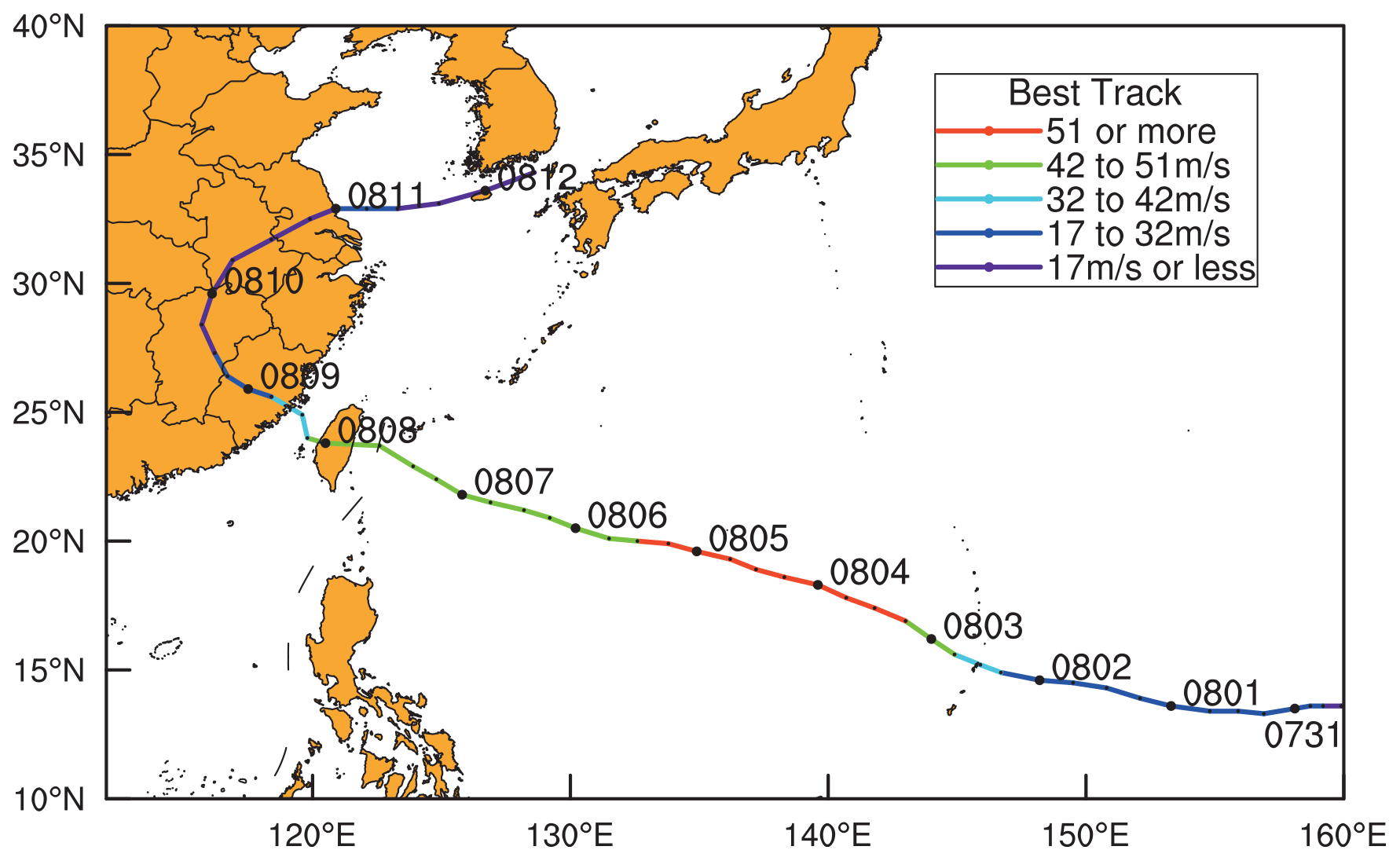
Figure 2 The best track of Soudelor from the China Meteorological Administration (CMA) from 00:00 UTC on 30 July to 06:00 UTC on 12 August 2015. Different colors represent intensity changes.

Figure 3 The time series of the minimum sea level pressure (solid line; unit: hPa) and the maximum surface wind (dashed line; unit: m s⁻¹) of Typhoon Soudelor from the CMA best-track data from 00:00 UTC on 30 July to 06:00 UTC on 12 August 2015. The specific period for the numerical results from 18:00 UTC on 1 August to 06:00 UTC on 4 August 2015 is highlighted in blue.

3.2 Experimental design

Two experiments are designed to investigate the effects of AHI radiance data direct assimilation on the analysis and forecast of Typhoon Soudelor from 18:00 UTC on 1 August to 00:00 UTC on 3 August 2015. WRF 3.9.1 is employed as the forecast model in this experiment. Arakawa C grid is used in the horizon with a 5 km grid distance. As is known, Arakawa A grid is “unstaggered” by evaluating all quantities at the same point on each grid cell. The “staggered” Arakawa B grid separates the evaluation of the velocities at the grid center and masses at grid corners. Arakawa C grid further separates evaluation of vector quantities compared to the Arakawa B grid. Vertically, it has 41η levels, using 10 hPa as its top with coarser vertical spacing for the higher levels. The center of the model domain is located at 17.5^∘ N, 140^∘ E (Fig. 4). The initial condition and lateral boundary are provided by $\mathrm{0.5}{}^{\circ }\times \mathrm{0.5}{}^{\circ }$ GFS reanalysis data. The following parameterization schemes are used: WDM6 microphysics scheme (Lim and Hong, 2010), Grell–Dévényi cumulus parameterization scheme (Grell and Dévényi, 2002), Rapid Radiative Transfer Model longwave radiation scheme (Mlawer et al., 1997), shortwave radiation scheme (Dudhia, 1989), and YSU boundary layer scheme (Hong et al., 2006).

Figure 4 Distribution of GTS observations in the simulated area at 00:00 UTC on 2 August 2015. On the right side of the map are the name of observation data and the number of observations. Each observation type is marked with a different color along with a unique symbol.

Figure 5 The flow chart of the data assimilation experiments. (a) CTNL, (b) AHI_DA.

The experimental procedures are illustrated by Fig. 5. Firstly, a 6 h spin-up is conducted, initialized at 18:00 UTC on 1 August 2015, to prepare the background field for the data assimilation at 00:00 UTC on 2 August 2015. The 6 h spin-up period is commonly applied to initialize the typhoon or hurricane system before the data assimilation experiments, although a longer spin-up period is also acceptable to introduce more model errors into the background, such as 12 or 24 h. The first experiment assimilates GTS (Global Telecommunications System) conventional data (including aircraft reports, ship reports, sounding reports, satellite cloud wind data, and ground station data) only, which is called the control experiment (CTNL). Another experiment is configured with AHI radiance data assimilation (AHI_DA). AHI radiance data are assimilated hourly further from 00:00 to 06:00 UTC on 2 August 2015. Afterwards, a 48 h forecast is launched as the deterministic forecast. The climatological background error (BE) statistics are estimated using the National Meteorological Center method. There are five control variables applied in this study, including U component, V component, full temperature, full surface pressure, and pseudo-relative humidity. The observation error for each channel is estimated based on the observed brightness temperature minus background brightness temperature (OMB) from 00:00 UTC on 1 August to 00:00 UTC on 3 August 2015 every 6 h.

Figure 6 (a) Cost function and (b) gradient as functions of iterations.

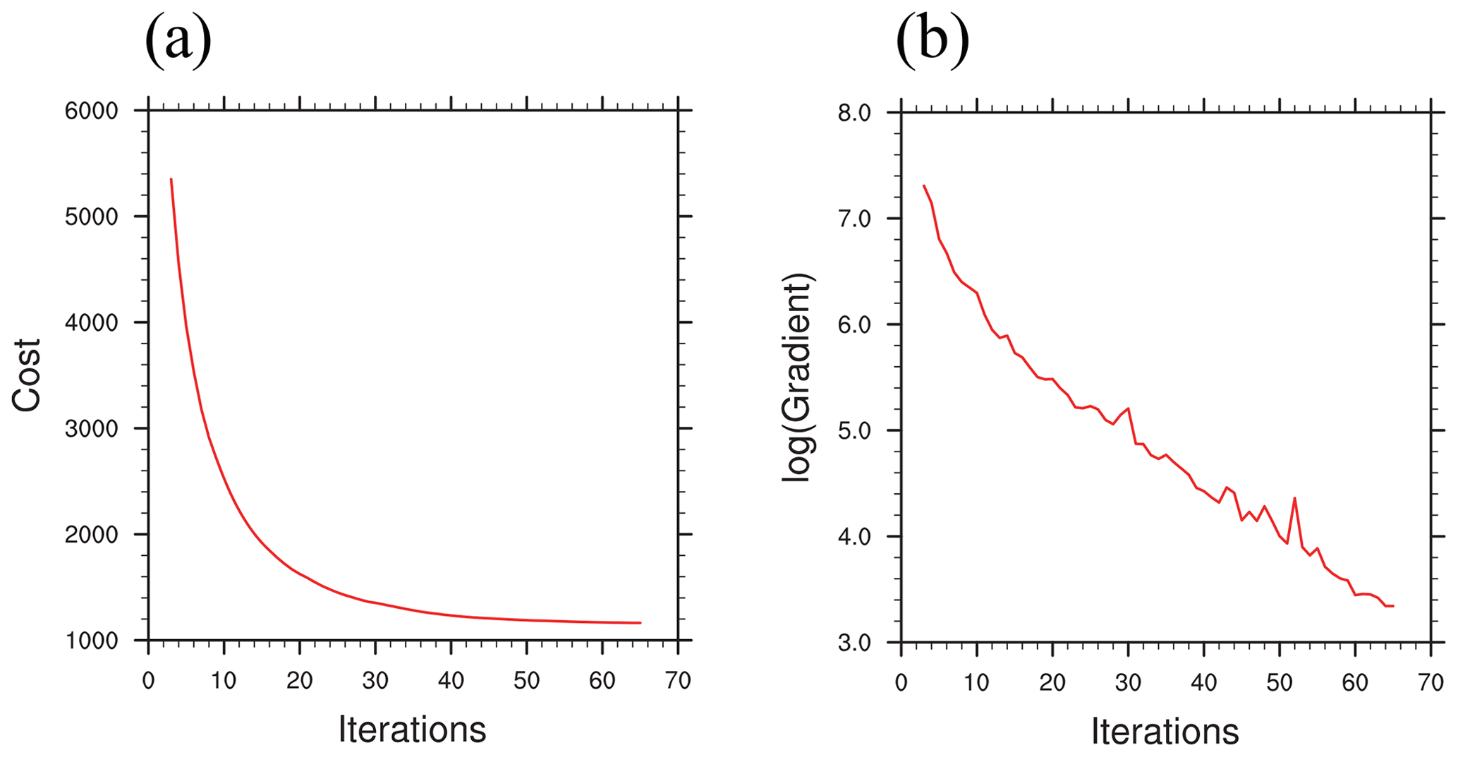
Figure 4 also shows the distribution of GTS observation data at the simulated domain at 00:00 UTC on 2 August 2015. It is proved that raw radiance observations thinned to a grid with 2–6 times the model grid resolution are able to remove the potential error correlations between adjacent observations (Schwartz et al., 2012; Xu et al., 2015; Choi et al., 2017). Hence, 20 km is chosen for thinning of AHI radiance data. Sensitivity experiments with a 25 and 30 km thinning mesh have also been conducted with similar results (Wang et al., 2018). The length scale and the variance scale are set to be 0.5 and 1, respectively, after several sensitivity experiments conducted on tuning the background error. Similar conclusions are also found in Shen and Min (2015) with the scale factors related to the static background error covariance.

4 Results

4.1 Minimization iterations

In this study, minimization stops when the norm of the gradient for the cost function is reduced by a factor of 0.01, which is commonly used in data assimilation procedures. Inner minimization stops either when the criterion of the cost function gradient is met or when inner iterations reach 200. Figure 6 shows the cost function and gradient with the iteration times. It is found that, for this case, the criterion of the cost function gradient decrease is met. There is an obvious exponential decrease curve in Fig. 6a, while Fig. 6b shows gradient decreases with the increase of iteration times. It is seen from Fig. 6a that the cost function decreases remarkably in the first 10 iterations. However, after 30 iterations, the cost function curve becomes smooth gradually. The differences between the background field and observation were largest. With continuous iterations, the background field goes through continued adjustments. Finally, the cost function tended to reach a stable minimum that represents the point when the cost function has its optimal solution. Furthermore, the gradient in Fig. 6b decreases generally with increasing iterations. The exponential decrease of the cost function and the change trend of its gradient indicate the effectiveness of AHI radiance DA. The final iterated analytical field was close to the observation. The wall clock times used by CTNL and AHI_DA for the data assimilation procedures are rather comparable with roughly 30 and 40 min on a Linux workstation with 36 processors. It should be pointed out that computational costs of the deterministic forecast and the pre-process for gridded GFS data are the same in these two experiments.

4.2 Analytical results of the brightness temperature

Figure 7a, c, and e show the distribution of OMB, while the observed brightness temperature minus the simulated brightness temperature from the analyses (OMA) after the bias correction of AHI radiance data are presented in Fig. 7b, d, and f from channels 8–10 at 00:00 UTC on 2 August 2015. It should be pointed out that, even when only parts of the AHI radiance data (roughly 20 000 clear-sky pixels of total 50 000 px for each DA cycle) are applied after quality control in the data assimilation, the radiative transfer model is able to simulate the brightness temperature for all the model grid points with the background and the analysis for verification purposes. The similar verification method is also applied in Yang et al. (2016). In Fig. 7a, part of the typhoon's spiral cloud belt is clearly visible. The brightness temperature in the typhoon's inner-core area was low, while the brightness temperature in other areas was high. The mean of observed OMB was −4.65 K, indicating that the background brightness temperature was higher than the observation. It is found in Fig. 7b that the OMA values of most pixels were below 0.02 K, indicating that the analytical field fitted the observation after analyzing. It can be inferred from Fig. 7a, c, and e that the magnitude in OMB of channel 10 was generally larger than that of channel 9, while that of the OMB in channel 8 was the smallest. This is because the detection height of channel 10 was lower than that of channel 8 and 9 as seen from the weighting function (Fig. 1), indicating channel 10 is largely affected by the clouds. Conversely, the weighting peak of channel 8 was the highest, being least affected by the clouds. In general, the simulated brightness temperature from the analyses matched well with the observed brightness temperature of all the three water vapor channels after the assimilation of AHI radiance data.

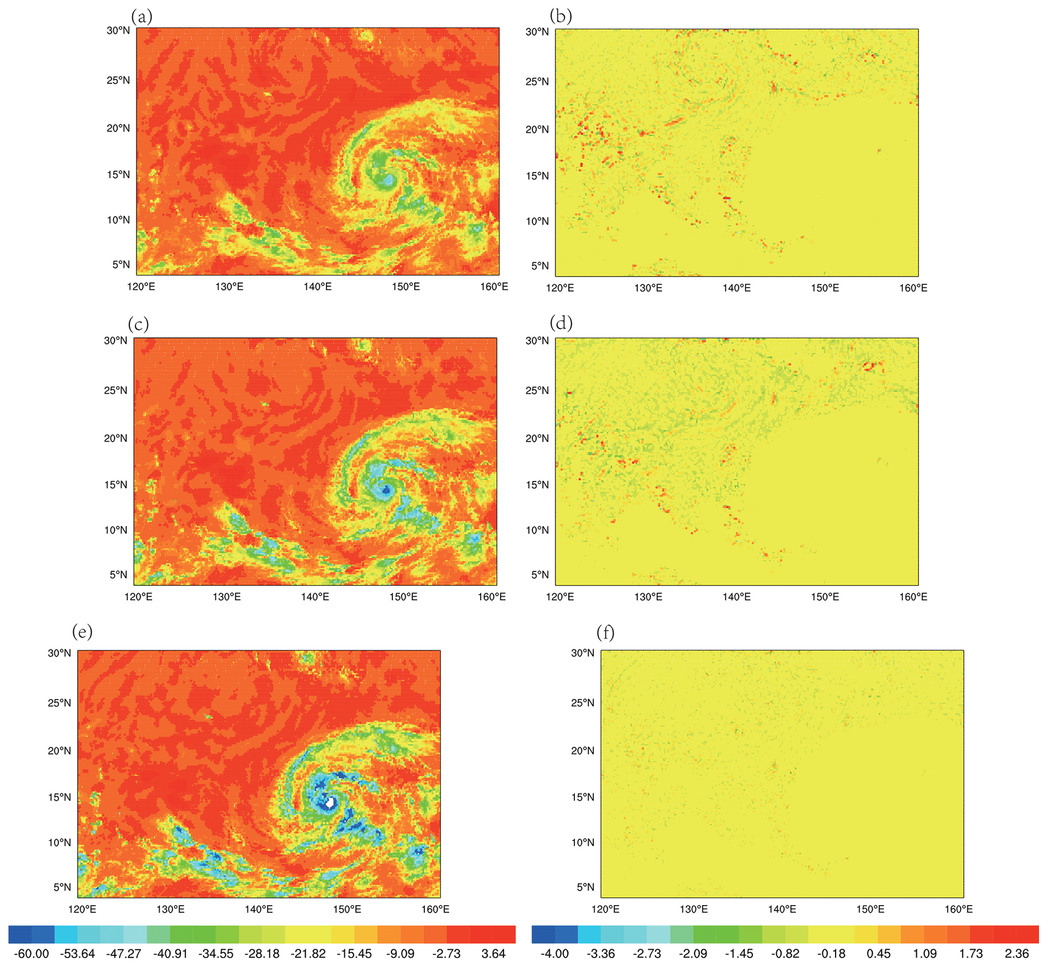
Figure 7 (a, c, e) OMB (unit: K) after bias correction for channels 8–10, respectively; (b, d, f) OMA (unit: K) after bias correction for channels 8–10, respectively, at 00:00 UTC on 2 August 2015.

To validate the effect of the bias correction for AHI radiance data at 00:00 UTC on 2 August 2015, the scatterplots of the observed brightness temperature and the brightness temperature from the background before the bias correction are shown in Fig. 8a, d, and g. Similarly, the results after the bias correction are provided in Fig. 8b, e, and h. From Fig. 8a, before the bias correction, the values from the observation and the background were comparable, but most of the scatter points were below the diagonal line. This suggests that the observed brightness temperature was higher than the background simulated brightness temperature. From Fig. 8b, after the bias correction, the observed warm bias was corrected to some extent, with the root mean square error (RMSE) of OMB decreasing from 1.864 to 1.627 K and the average decreasing from 0.956 to 0.358 K. The scatterplots of the observed brightness temperature and the brightness temperature from the analyses after the bias correction are shown in Fig. 8c, f, and j. Compared to the result of Fig. 8b, the scatters in Fig. 8c were more symmetrical, fitting closely to the diagonal line. The mean and RMSE were also significantly reduced, suggesting that the analytical fields match better with the observation than background field. Among them the RMSEs of channel 10 are smallest compared to those from channels 8 and 9 for the OMB and OMA samples, which is likely related to the strict cloud detection scheme for channel 10 with a rather lower detection peak (Wang et al., 2018).

Figure 8 Scatterplots of (a, d, g) the observed and background brightness temperature before the bias correction of channels 8–10. Scatterplots of (b, e, h) the observed and background brightness temperature after the bias correction of channels 8–10. Scatterplots of (c, f, i) the observed and analyzed brightness temperature after the bias correction of channels 8–10.

Figure 9 shows the observation numbers, the mean, and the standard deviation of OMB and OMA of channels 8–10 before and after the bias correction. It can be seen that after the quality control 24 057, 24 181, 21 785 observations are adopted in the DA system for channels 8–10, respectively. From the mean value of OMB before the bias correction, the value of the three channels was relatively small, indicating that the simulated brightness temperature of the three channels was close to the observed brightness temperature. The lowest mean of 0.3 K was found in channel 10, indicating that the simulated brightness temperature of channel 10 was closest to the observed brightness temperature. Bias correction effectively corrects the systematic bias and reduces the mean value of observation residuals. After the bias correction, the OMB mean value of the three channels significantly decreases to nearly 0 K. With the bias correction, the simulated brightness temperature was almost the same as the observed brightness temperature. The standard deviations of OMB were comparable before and after the bias correction, since they are calculated by subtracting the mean of the bias. It is found that the bias was corrected effectively with the same magnitude of bias overall for each pixel, resulting in the standard deviation being almost same before and after the bias correction. The standard deviation of OMA decreased by about 80 % compared to OMB, indicating that the analyses fit better with the observations after the data assimilation. Differences between the standard deviations of the OMB and OMA were statistically significant at the 95 % level using zero difference for the null hypothesis.

Figure 9 (a) Number of observations, (b) mean (unit: K), and (c) standard deviations (unit: K) of OMB and OMA before and after the bias correction for water vapor channels 8–10 (OMB_nb: OMB without bias correction; OMB_wb: OMB with bias correction).

The RMSEs of the simulated brightness temperature by the NWP model before and after the assimilation are also calculated against the AHI radiance observations. Figure 10 shows the RMSEs during the DA cycles for channels 8–10. As can be seen from Fig. 10, RMSE decreased after each analysis in AHI_DA. The most significant improvement was from the first analysis cycle of channel 8, where RMSE of the brightness temperature after assimilation significantly decreases from 1.64 to 0.46 K, possibly due to the largest adjustment on the background for the first analysis time. The background before the assimilation was the short-term forecast from the previous analysis. The increase of the RMSE in the fluctuation arose from the model error in the 1 h short-term forecast. Overall, the effect of the analysis from channel 10 was most significant.

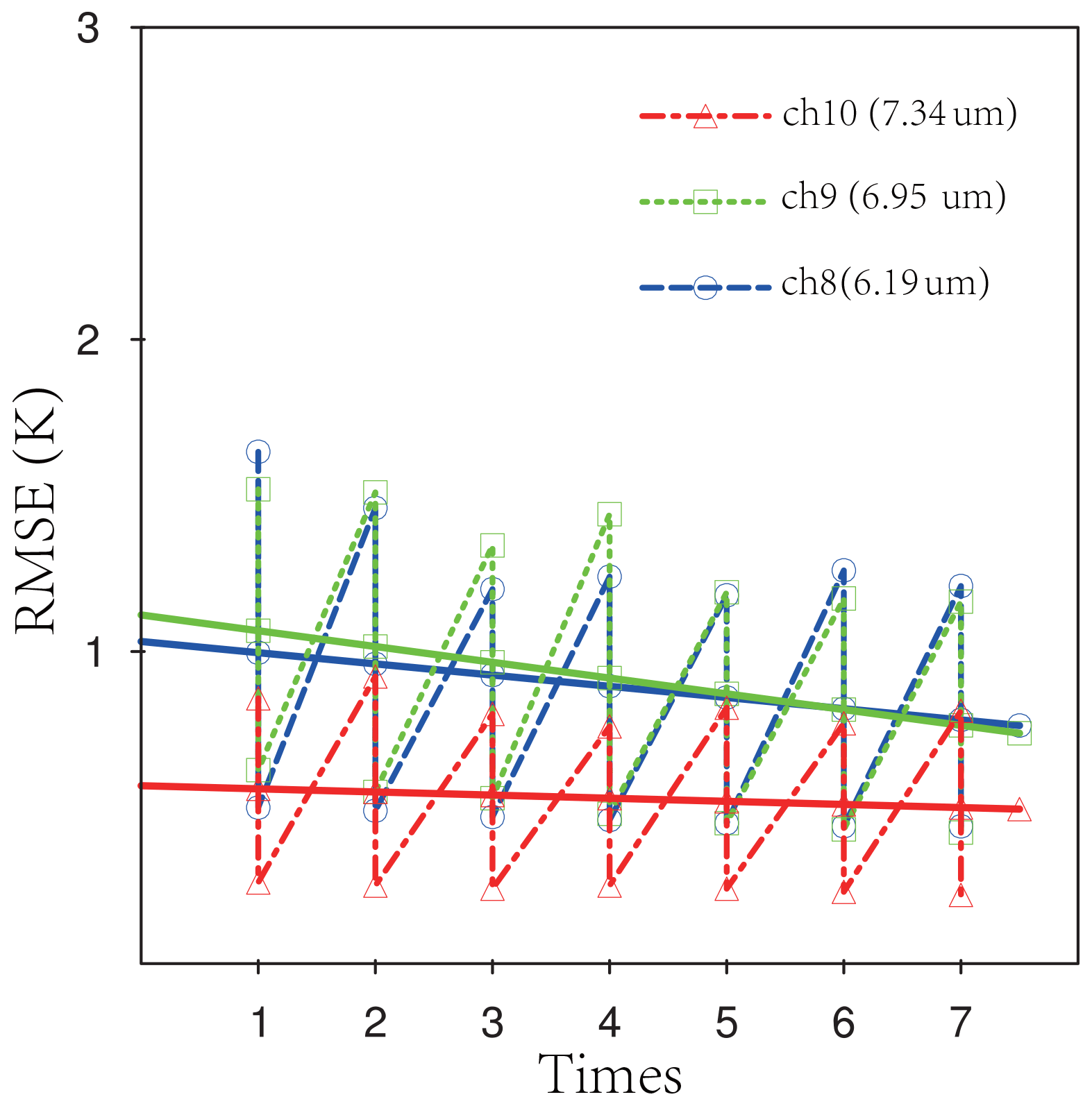
Figure 10 Time series of the RMSE for the brightness temperature (unit: K) with assimilation times before and after the data assimilation along with the trend lines.

4.3 Analysis of the typhoon structure

Figure 11 shows the wind field at sea level and the distribution of water vapor at 850 hPa at 00:00 UTC on 2 August 2015. The obvious cyclonic eddy circulation structures in the core area of the typhoon are found in both fields, while the anti-cyclonic circulation existed in the northwest quadrant of the typhoon. The mixing ratio of water vapor in the region where the typhoon was located was very high, and the wind field was cyclonic, indicating that the typhoon had a continuous water vapor advection. This contributed to the enhancement of the typhoon (Kamineni et al., 2003). From the flow field of the control experiment in Fig. 11a, the water vapor convergence in the center of the typhoon region was weak with the low intensity and smaller coverage. As can be seen from Fig. 11b, after the assimilation of AHI radiance data, the streamlines in the typhoon region become denser, indicating that the cyclonic circulation was strengthened. Conversely, the intensity and distribution of the water vapor after the assimilation of AHI radiance data tend to contribute to the developing typhoon. This suggests that the field outside of the typhoon center was also adjusted as the assimilation of AHI radiance data was able to improve the large-scale environmental field in the simulation region of Typhoon Soudelor. It should be pointed out that the model status in the cloudy area was modified due to the spatial correlation in the background error covariance. The similar findings for small-scale information in the cloudy area can also be referred to in Wang et al. (2018).

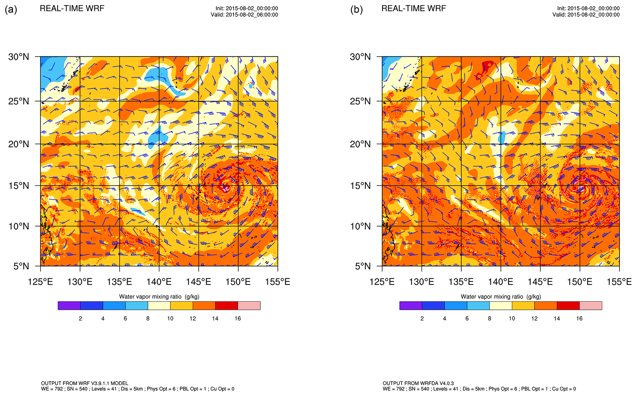
Figure 11 The surface wind speed (vectors; unit: m s⁻¹) and water vapor (colored; unit: g kg⁻¹) for (a) CTNL and (b) AHI_DA at 850 hPa at 00:00 UTC on 2 August 2015.

4.4 Track forecast

In order to further evaluate the effect of AHI radiance data assimilation, a 48 h deterministic forecast was launched with the analyses initialized from 00:00 UTC on 2 August and 06:00 UTC on 2 August 2015. The best track data are provided by the CMA (Yu et al., 2007; Song et al., 2010). The improvement is most obvious at the start and end point. As can be seen in Fig. 12a, at the beginning of the forecast, the initial location of the typhoon from the CTNL experiment has a large south bias and east bias at 00:00 and 06:00 UTC, respectively. Conversely, the location of the typhoon in AHI_DA is relatively closer to the observation at the beginning. During the following few hours of forecasts, the typhoon track predicted by the CTNL continues to show a southwest bias with the environmental wind, while the track predicted by AHI_DA matches better with the best track. Figure 12c shows the averaged typhoon track error over the two forecasts predicted by the two experiments. At the initial time of the forecast, the track errors of CTNL and AHI_DA were significantly different, with a magnitude of 55.6 and 13.4 km, respectively. During the subsequent 48 h forecast, the track error of the CTNL gradually increases with the forecast time, reaching 167.1 km at the end of the forecast. In contrast, the track error of AHI_DA is consistently less than 122.5 km during the 48 h forecast period. In general, the average track error of the CTNL is 168.57 km, and the average track error of AHI_DA experiment is only 67.0 km, indicating a significant improvement in the track prediction.

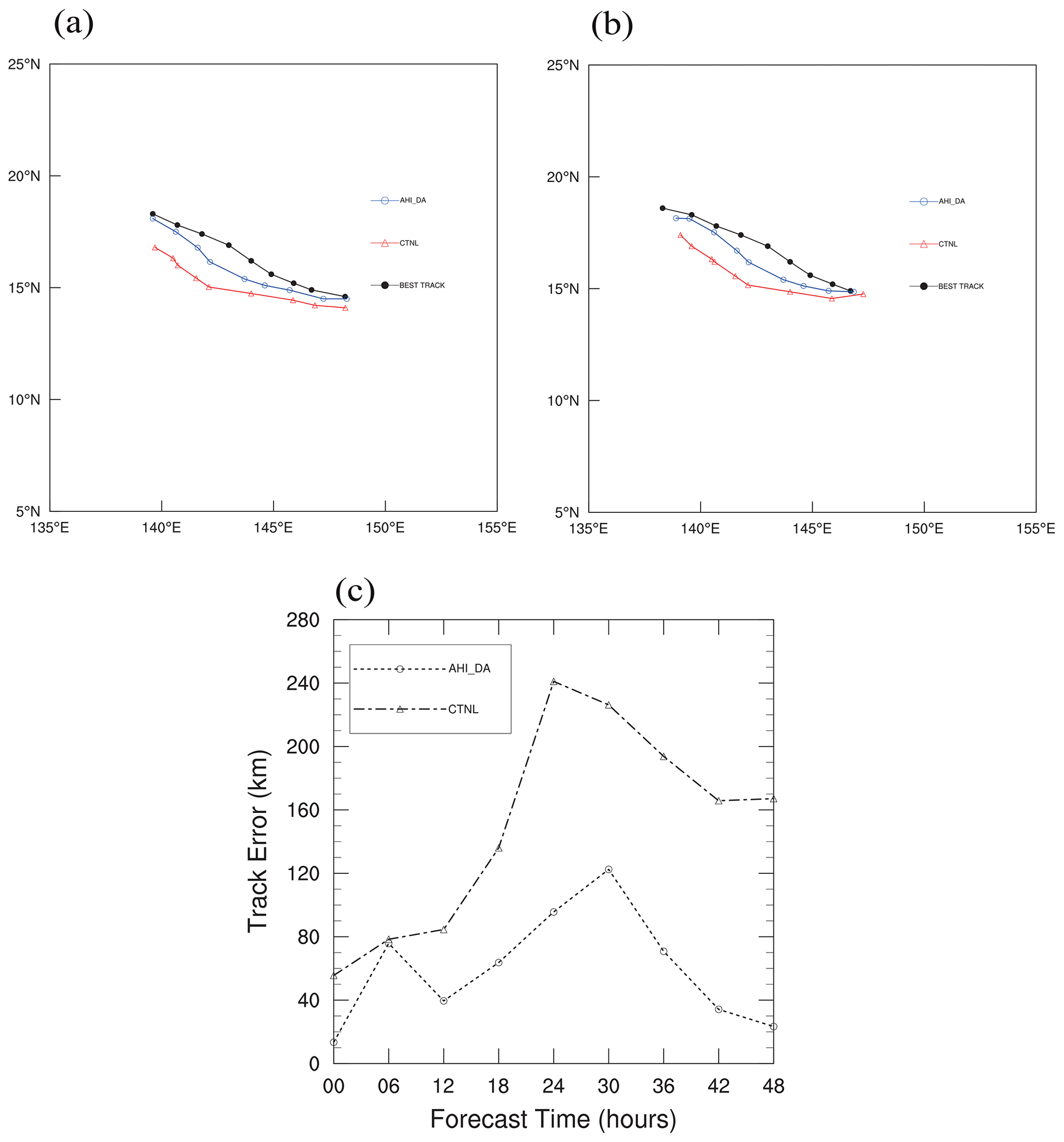
Figure 12 The 48 h predicted tracks (a) from 00:00 UTC on 2 August to 00:00 UTC on 4 August and (b) from 06:00 UTC on 2 August to 06:00 UTC on 4 August 2015; (c) averaged track errors (unit: km) for the two forecasts.

Figure 13 provides the time series of the typhoon intensity from the two experiments in terms of the averaged maximum surface wind and minimum sea level pressure error over the two forecasts initialized from 00:00 UTC on 2 August and 06:00 UTC on 2 August 2015, respectively. It can be seen that the maximum surface wind error predicted by the AHI_DA was much lower than that by the CTNL for the first 30 h, due to the overall underestimation for the intensity of Typhoon Soudelor simulated in the background field. The maximum surface wind errors of AHI_DA are generally smaller than those of CTNL. It should be pointed out that the difference between the maximum surface wind errors of the two experiments reaches up to 7.5 m s⁻¹ after 24 h forecast. In Fig. 13b, the results of the minimum sea level pressure are consistent with Fig. 13a, while the improvement for the minimum sea level pressure lasts for 40 h.

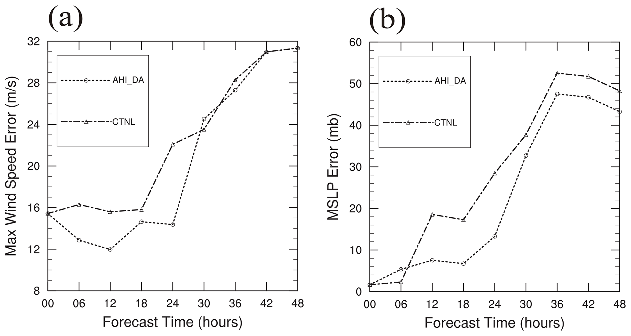
Figure 13 The 48 h (a) maximum surface wind error (unit: m s⁻¹) and (b) minimum sea level pressure error (unit: hPa) of Soudelor (2015) averaged from two forecasts.

5 Conclusion

An interface for AHI radiance data assimilation in the WRFDA system based on the 3DVAR assimilation method was built. Based on Typhoon Soudelor in 2015, two experiments for comparison were designed to examine the impact of AHI water vapor channel radiance data assimilation on the analysis and prediction of the rapid development stage of Typhoon Soudelor under clear-sky conditions. Following conclusions are obtained:

1. The AHI radiance data on the new-generation geostationary meteorological satellite is able to reflect the structure of Typhoon Soudelor very clearly. After a series of pre-procedures such as quality control and bias correction, cloudy pixels are able to effectively be eliminated, ensuring the validity and rationality of the AHI radiance data. The biases are also eliminated from the VarBC statistical method, which is able to provide a positive impact on the data assimilation procedure for the typhoon numerical simulation.

2. Compared with the control experiment with only GTS data, the 3DVAR assimilation including AHI radiance data is able to improve the structure of the typhoon's core and outer rain band. Also, the position and intensity of the typhoon in the background field are able to be corrected.

3. Generally, the track and minimum sea level pressure from the AHI radiance data assimilation experiment match better with the best track than the control experiment does for the subsequent 48 h forecast. The maximum surface wind forecast error is reduced only for the first 30 h.

In this study, the AHI water radiance data assimilation is conducted under clear-sky conditions. The results of the experiments indicate that AHI radiance data assimilation has a positive effect on the analysis and prediction of rapidly intensifying TC. Although all development stages of Typhoon Soudelor include a rapid intensification, a weakening, and a second intensification, only the first intensification during 1 to 4 August is considered as the numerical period. It is worth investigating the impact of AHI data assimilation on the whole period, including the first intensification, the weakening, and the second intensification of Typhoon Soudelor to fully prove the advantages of AHI radiance data assimilation. Considering the complex influence of the underlying surface, only the rapid development stage of a typhoon at sea was studied, while the whole generation, development, and disappearance stage of typhoons can also be studied in the future. In addition, based on the AHI radiance data of the water vapor channels under clear-sky conditions, only the 3DVAR method was adopted. Further improvements under all-sky conditions and hybrid DA can be obtained in the future.