Probabilistic landslide susceptibility analysis in tropical mountainous terrain using the physically based r.slope.stability model

Landslides triggered by rainfall are very common phenomena in complex tropical environments such as the Colombian Andes, one of the regions of South America most affected by landslides every year. Currently in Colombia, physically based methods for landslide hazard mapping are mandatory for land use planning in urban areas. In this work, we perform probabilistic analyses with r.slope.stability, a spatially distributed, physically based model for landslide susceptibility analysis, available as an open-source tool coupled to GRASS GIS. This model considers alternatively the infinite slope stability model or the 2.5-D geometry of shallow planar and deep-seated landslides with ellipsoidal or truncated failure surfaces. We test the model in the La Arenosa catchment, northern Colombian Andes. The results are compared to those yielded with the corresponding deterministic analyses and with other physically based models applied in the same catchment. Finally, the model results are evaluated against a landslide inventory using a confusion matrix and receiver operating characteristic (ROC) analysis. The model performs reasonably well, the infinite slope stability model showing a better performance. The outcomes are, however, rather conservative, pointing to possible challenges with regard to the geotechnical and geo-hydraulic parameterization. The results also highlight the importance to perform probabilistic instead of – or in addition to – deterministic slope stability analyses.

1 Introduction

Landslides cause substantial human and economic losses every year (Kjekstad and Highland, 2009; Petley, 2012; Schuster and Highland, 2001). According to Dilley et al. (2005), the worldwide area exposed to landslides is around 3.7 million km², within which 66 million people live in 820 000 km² identified as the high-risk zone. Petley (2008) mentioned that in 2007, 89.6 % of the fatalities due to landslides worldwide were related to rainfall-triggered landslides. Although economic losses tend to concentrate in industrialized and developed countries, the numbers of human fatalities and affected persons are highest in densely populated, less developed countries (Petley, 2012; Sepúlveda and Petley, 2015).

Landslides triggered by rainfall are a frequent phenomenon in mountainous terrain (Keefer et al., 1987; Van Westen et al., 2008; Varnes, 1978). In tropical environments and complex terrain such as the Colombian Andes a high percentage of landslides are triggered by heavy or prolonged rainfall (Van Westen and Terlien, 1996; Terlien, 1998). Specially the shallow landslides triggered by rainfall are very common phenomena in Colombia, where hillslopes are characterized by deep weathering profiles and are subjected to periods of intense tropical rainfall (Aristizábal, 2013). Colombia, due to its location in the northwestern corner of South America, exhibits complex geographical and hydro-climatological features arising from its tectonic setting and equatorial location. The mountainous configuration is the result of the Caribbean Plate moving southwestward relative to the South American Plate and the eastward subduction of the Nazca Plate beneath the northern Andes along the western margin of Colombia (Kellogg et al., 1995; Taboada et al., 2000; Trenkamp et al., 2002). Rainfall in Colombia is highly intermittent in space and time, due to the link between the hydro-climatological conditions and equatorial location; rainfall is influenced by the atmospheric circulation patterns over the neighboring tropical Pacific Ocean and the Caribbean Sea and the combined hydro-climatic and ecological dynamics of the Amazon and Orinoco basins (Poveda et al., 2007).

In Colombia, landslide-prone regions are densely populated. As a consequence, hundreds of fatalities are associated with landslides triggered by rainfall every year (Sanchez and Aristizábal, 2018). Being one of the countries most affected by landslides in South America, there is a strong social and economic need to include landslide susceptibility and hazard zoning in land use planning to reduce landslide fatalities and economic losses.

According to the Emergency Events Database (EM-DAT, 2011), Colombia is one of the South American countries with most landslides. In the period between 1901 and 2017, 45 landslide disasters were registered with 3619 fatalities, 78 395 people affected, and economic losses of USD 2.4 million. In the Global Landslide Catalog, Colombia has 87 entries with a total of 464 deaths (Kirschbaum et al., 2015) from 2007 to 2013. The Latin America and Caribbean landslide database has compiled a record of 110 fatal landslides in Colombia between the years 2004 and 2013 with a total of 880 deaths; Colombia is the country with the second highest number of fatal landslides in Latin America and Caribbean, only Brazil shows a slightly higher number (119; Sepúlveda and Petley, 2015). Mergili et al. (2015) show that Colombia, according to EM-DAT, presents a victim ∕ event ratio of 77.34 (3171∕41) and is only exceeded by Peru and Ecuador in this respect. However, the EM-DAT database only considers events with high numbers of fatalities: actually, the real number of fatal landslides is much higher (Aristizábal and Gómez, 2007; Mergili et al., 2015).

Landslide susceptibility assessment can be determined by qualitative or by quantitative methods (Corominas et al., 2014). Qualitative methods correspond to knowledge-driven approaches based entirely on the judgment of experts using geomorphological criteria in the field (Van Westen et al., 2000). Quantitative approaches are subdivided into data-driven methods and physically based models. Statistical or data-driven methods evaluate the relationship between landslides and causative factors to predict the landslide spatial probability (Carrara, 1983; Gorsevski et al., 2000; Lee, 2005; Lee and Pradhan, 2007; Süzen and Doyuran, 2004). Physically based models for landslide susceptibility and hazard assessment of detailed areas include the interaction between hydrology, topography, soil properties, and in some cases, vegetation in order to understand and predict the location and timing of landslide occurrence. Such models generally compute slope stability, using the factor of safety (FoS). FoS is given by the dimensionless ratio between the resisting forces and the driving forces (Lam and Fredlund, 1993). Most of the physically based models available in the literature build on the limit equilibrium concept and the assumption of a planar slope of infinite length with a potential failure surface parallel to the topographic surface (Chen and Chameau, 1983; Lam and Fredlund, 1993). However, the infinite slope stability approach is proposed only for shallow, planar sliding surfaces in friction-dominated soils and fails to capture the complexity of deep-seated landslide phenomena (Bishop, 1954; Carson and Kirkby, 1972; Crozier, 1986; Duncan and Wright, 2005).

Limit equilibrium models have been extended to three-dimensional (3-D) failure surfaces: geometric shapes such as spheres or ellipsoids represent non-planar slip surfaces in a much better way and are important to consider in areas of complex lithological conditions or for soils with high cohesion values. The first 3-D slope stability model was presented by Baligh and Azzouz (1975). Later, Chen and Chameau (1983) developed a method to analyze cohesive and frictional slopes with different pore water conditions. Dennhardt and Forster (1985) proposed a method using an ellipsoidal slip surface. Kalatehjari and Ali (2013) carried out a review of different 3-D analysis models in which they demonstrated the fact that many of the methods considered the slope and slip surface as symmetrical shapes in order to determinate the static condition of equilibrium. Hovland (1997) presented a method for cohesive and frictional soils based on the Fellenius method (Fellenius, 1927). In this approach, the forces that act between columns are disregarded and FoS is determined by normal and shear forces that act at the bases of the columns (Lam and Fredlund, 1993).

Although FoS represents a quantitative – and seemingly objective – approach to evaluate slope stability, it has to be used carefully. Authors such a Kirsten (1983) mention that different values of FoS could be obtained from slopes with equal probability of failure. Several software packages use this concept for 3-D slope stability analysis, e.g., STAB3D (Baligh and Azzouz, 1975), 3D-PCSTABL (Thomaz, 1986), CLARA (Hungr, 1988) and TSLOPE3 (Pyke, 1991). Most of these models include some limitations reducing the accuracy of FoS obtained (Stark and Eid, 1998). One of the most important limitations is that they were designed to analyses individual landslides or slopes; they are not appropriate for regional or catchment-scale slope stability analyses (Mergili et al., 2014b). A few 3-D (or, strictly speaking, 2.5-D) slope stability models in geographic information systems (GIS) have been used for landslide susceptibility mapping (Carrara and Pike, 2008; Qiu et al., 2007; Xie et al., 2003). In terms of scale or spatial resolution, physically based models have been suggested to be applied to finer-scale study areas, and their results are strongly influenced by the level of detail in the input data (Zizioli et al., 2013), whereas data-driven approaches are recommended for broader-scale landslide susceptibility analyses (Van Westen et al., 2006; Corominas et al., 2014). In fact, the implementation of data-driven methods or physically based models for the incorporation of landslide hazard mapping into land use planning has been regulated in several countries. Recently, the r.slope.stability model, a C- and Python-based raster module in the open-source software GRASS GIS (GRASS Team, 2019) has been proposed. The r.slope.stability model considers the 2.5-D geometry of the sliding surface for analyzing a number of randomly selected potential sliding surfaces that are ellipsoidal or truncated in shape (Mergili et al., 2014a, b), and also offers an implementation of the infinite slope stability model.

In Colombia, according to Decree 1807/2014, the implementation of deterministic or probabilistic physically based methods are obligatory in urban and urban expansion areas, whereas statistical- and knowledge-driven models are only permitted for rural areas.

In order to meet this requirement, we have to obtain more detailed knowledge on the suitability of the available physically based landslide susceptibility models, with the final goal of using model ensembles in order to obtain a broader, more robust picture of landslide susceptibility conditions. We think that r.slope.stability is a suitable tool for calculation of unstable areas in tropical environments, considering shallow planar and deep-seated ellipsoidal failure surfaces. Consequently, the scientific aims of the present study are (i) to evaluate the suitability of r.slope.stability for physically based landslide susceptibility mapping in tropical mountainous terrain, and (ii) to identify its fit with other potentially suitable models, helping to learn about strengths, limitations and uncertainties.

Following these aims, we present a probabilistic analysis of slope stability in GIS for modeling landslide susceptibility in a tropical and mountainous environment using the r.slope.stability model. This model is evaluated using a landslide inventory prepared after a major and destructive rainfall-triggered multi-landslide event in the La Arenosa catchment on 21 September 1990. A quantitative performance evaluation of the model by receiver operating characteristic (ROC) analysis is carried out. The results are compared with those obtained through the corresponding deterministic analyses with r.slope.stability, with SHALSTAB (Dietrich and Montgomery, 1998) and with SHIA_Landslide (Aristizábal et al., 2016), which represents a new model developed for tropical mountainous terrain.

2 Study area

The La Arenosa catchment, with an area of 9.9 km², is located on the northwestern side of the Colombian Andes, at 1000–1900 m a.s.l. (above sea level; Velásquez and Mejía, 1991; Aristizábal et al., 2016). The climate is tropical humid with a mean annual temperature of 23 ^∘C and a mean annual precipitation of 4300 mm. However, precipitation is highly variable between the different seasons and between years. The annual cycle of precipitation shows a bimodal period of rainfall (interannual scale) with rainfall peaks in the months of April (450 mm) and October (600 mm; IDEAM, 2010). Rainfall often occurs in the afternoon and at night in the form of heavy rainstorms or cloudbursts of short duration (Aristizábal et al., 2015; Garcia, 1995). Most of the landslides in the catchment are triggered by such events and by the variation of groundwater level due to antecedent rainfall conditions, which is decisive for the occurrence of landslides (Fressard et al., 2016).

Although the natural vegetation of the La Arenosa catchment would normally be very humid premontane forest, all primary forest has been removed, and the land is exclusively dedicated to agricultural use. In the highest and steepest parts of the basin, the predominance of coffee crops, sugar cane, pastures and very small areas of secondary forest is maintained; this situation is considered a factor that influences the stability of the slopes in the catchment (Aristizábal, 2013).

Residual soils which have evolved from granodiorite rocks covered by slope deposits and fluvio-torrential deposits are characteristic for the area. Slope deposits cover approx. 15 % of the catchment. Strong in situ weathering occurs due to chemical decomposition in the humid tropical climate (Velásquez and Mejía, 1991). Indicators of rapid, extensive and progressive spheroidal decomposition of the granite are observed down to an average depth of 30 m. The saprolite is fairly well graded. Its texture is described as sandy silt or silty sand with some gravel and a small fraction of clay. Relict joints in the parent rock are preserved in the saprolite. They facilitate preferential flow and therefore strongly influence the observed hydraulic conductivity of the surrounding soil matrix (INTEGRAL, 1990; Aristizábal et al., 2015). The matrix-supported slope deposits are formed by boulders of granite, residual soils and vegetation debris (Aristizábal et al., 2015). Slope deposits generally accumulate at foot slopes or in gullies. Those usually poorly consolidated deposits are the consequence of past landslides. Their content in cobbles and boulders is high, and natural soil pipes are common (Velásquez and Mejía, 1991).

On 21 September 1990, the La Arenosa catchment was strongly affected by a rainfall event of high intensity and short duration. In less than 3 h, 208 mm of precipitation, with a maximum intensity of 90 mm h⁻¹, was recorded within the study area, triggering approximately 800 landslides. Based on the intensity–duration–frequency (IDF) curve, a return period of 200 years was estimated for this event (Velásquez and Mejía, 1991).

The strong rainfall in the catchment, imposed upon general saturation of the soils in rugged topography, triggered a series of almost simultaneous rotational and translational landslides in the catchment (Hermelin et al., 1992; Garcia, 1995). A total of 699 landslides were identified and mapped in the La Arenosa catchment. However, although the inventory map is very precise on the locations of events, there is no information available which permits differentiation between translational and rotational landslides. According to Velásquez and Mejía (1991), most of the landslides started as shallow translational slides and transformed into debris flows, from very rapid to extremely rapid, with high water content (Fig. 1). The landslide bodies were small with respect to the flow length, and the slip surfaces were parallel to the slope surface. The majority of the landslides initiated within residual soils in hollows and open slopes with a slope steepness ranging from 35 to 42^∘ (Velásquez and Mejía, 1991). The same authors described that the depth of failure surface was less than 3 m and corresponded to the contact of the residual soil with the saprolite.

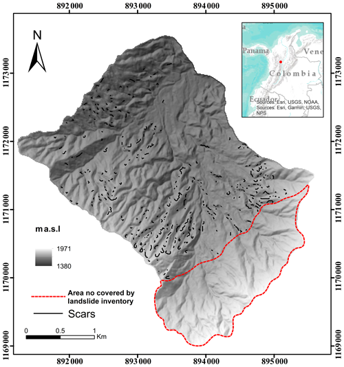
Figure 1 Landslides scars inventory database according to landslide inventory. The area with a red line does not have a landslide inventory. Source: adapted from INTEGRAL (1990) and Velásquez and Mejía (1991).

The population was strongly affected: 20 fatalities were counted and 260 people had to be evacuated, 27 houses were destroyed and 30 damaged and several bridges were also damaged or destroyed (Hermelin et al., 1992; Aristizábal et al., 2016). Total loss was estimated to be more than USD 6 million.

INTEGRAL (1990) with Velásquez and Mejía (1991) analyzed a set of aerial images and conducted a detailed field survey to produce a detailed landslide inventory for the event. However, it was not feasible to generate a complete inventory of landslides for the entire catchment as aerial photographs and topographic maps were not available for an area of approx. 2 km². Only the area covered by the landslide inventory was considered for this study, corresponding to an area of 7.6 km².

3 The r.slope.stability model

The r.slope.stability model is a GIS-based, free and open-source slope stability modeling software (http://www.slopestability.org/, last access: 31 May 2018) developed by Mergili et al. (2014a, b) as a C- and Python-based raster module of the GRASS GIS software package (GRASS Team, 2019). The tool is able to take into account planar failure with an infinite slope stability module and a slip surface module.

For shallow and planar landslides, r.slope.stability includes a classic infinite slope stability approach. For the infinite slope stability analysis, S acts parallel to the shear plane and seepage is considered parallel to the slope. For ellipsoid-shaped slip surfaces, in contrast, S is generally not parallel to the shear plane of the columns, even if it is parallel to the slope (Mergili et al., 2014b). The infinite slope stability model is run independently from the ellipsoidal failure surface analysis: FoS_inf for each raster cell is calculated according to Eq. (1).

$$\begin{array}{}\text{(1)}& {\mathrm{FoS}}_{\inf }={\displaystyle \frac{c^{\prime }\cdot A+G^{\prime }\cos \mathit{\beta }\tan {\mathit{\phi }}^{\prime }}{G^{\prime }\cos \mathit{\beta }+S}},\end{array}$$

where β is the slope angle of the slip surface (corresponding to the inclination of the terrain).

The slip surface model considers the 2.5-D geometry of the sliding surface and evaluates FoS or the probability of slope failure (P_f) for many randomly selected potential ellipsoidal or truncated slip surfaces (Fig. 2). Each raster cell can be affected by various slip surfaces and is characterized by a unique value of FoS or P_f for each raster cell of the study area. Thereby, the most relevant values for each cell analyzed are the lowest value of FoS and the highest value of P_f. The model permits users to impose restrictions with respect to the width, length and depth of the ellipsoids (Mergili et al., 2014a, b).

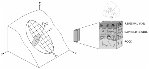
Figure 2 The typical ellipsoid used, slip surface with a model column in r.slope.stability and a typical weathering profile of tropical environments and complex terrains. Source: adapted from Aristizábal et al. (2016) and Qiu et al. (2007).

The slip surface model used in r.slope.stability represents a revision and extension of the 2.5-D sliding surface model of Hovland (1997; Xie et al., 2003). The calculation of FoS is based on the basic principle of equilibrium (Eq. 2).

$$\begin{array}{}\text{(2)}& \mathrm{FoS}={\displaystyle \frac{\sum \left(c^{\prime }\cdot A+\left(G^{\prime }\cos {\mathit{\beta }}_{\mathrm{c}}+N_{\mathrm{s}}\right)\tan {\mathit{\phi }}^{\prime }\right)\cos {\mathit{\beta }}_{\mathrm{m}}}{\sum \left(G^{\prime }\sin {\mathit{\beta }}_{\mathrm{m}}+T_{\mathrm{s}}\right)\cos {\mathit{\beta }}_{\mathrm{m}}}},\end{array}$$

where c^′ is the effective cohesion (N m⁻²), G^′ is the weight of the moist soil (N), β_c is the inclination of the slip surface, φ^′ is the effective internal friction angle, β_m is the apparent dip of the sliding surface in direction of the aspect α, N_s and T_s (N) are the contributions of the seepage force to the normal force and the shear force, respectively, and A (m²) is the slip surface area assigned to each column. Inter-column forces and external forces (e.g seismic loading) are neglected (Mergili et al., 2014a, b). The slip surface model is further based on the model of King (1989), in which the direction of the seepage force (S) corresponds with the direction of the hydraulic gradient, approximated by slope and aspect of the groundwater table.

Both the infinite slope stability model and the slip surface model can be used for a probabilistic analysis, applying a range of geotechnical parameters (c', φ^′) and the depth of the failure surface. Rectangular, normal, log-normal or exponential probability density functions can be used with r.slope.stability. The result is a probability of failure (P_f), representing the fraction of tested parameter combinations yielding FoS < 1 (Mergili et al., 2014a).

Note that, in the present work, with probabilistic model, we always refer to the random variation of the geotechnical parameters. The slip surface model includes a probabilistic component where the dimensions of the ellipsoids are randomly varied for the computation of FoS.

4 Data and procedure

The input of the r.slope.stability model consists of a digital terrain model (DTM), spatial datasets of the mechanic and hydraulic characteristics of the study area, and finally the restraints imposed to the model by the user, based on the knowledge of the study area. A DTM with a spatial resolution of 10×10 m was provided by the Instituto Geográfico Agustín Codazzi. A soil thickness map was built using interpolation, employing an empirical relationship between soil thickness and slope angle in the study area (Aristizábal, 2013; Catani et al., 2010; Thiery et al., 2019). The computed residual soil depth ranges from 1 to 2.8 m.

The La Arenosa catchment is basically composed of two soil types, alluvial and residual, with properties strongly related to the parental material (IGAC, 2007). Alluvial soils cover 6.7 % of the total area; they correspond to quaternary deposits composed of alluvial sediments of moderate depth, limited by the presence of fragments of rock and gravel. Residual soils cover 93.3 % of the total area; they are derived from igneous rocks such as granites and quartz-diorites. The residual soils are medium-to-fine textured, well-drained and in some cases characterized by gravel or stones in the profile. These soils have deep weathering profiles depending on parent rock lithology and local conditions, partly reaching down to a depth of 100 m (Aristizábal et al., 2005; Suarez, 1998). The geotechnical parameters were obtained based on studies and laboratory tests carried out in La Arenosa by Velásquez and Mejía (1991). For the residual soils, cohesion values range between 5 and 12.5 kPa, whereas the internal friction angle of the soil ranges from 16 to 24^∘. The dry unit weight ranges from 14.3 to 14.9 kN m⁻³. No geotechnical laboratory tests are available for the alluvial deposits; however, they show very gentle slopes generally not prone to landslides; the cohesion and friction angle values were therefore assumed based on literature values (Ameratunga et al., 2016; Aristizábal, 2013; Aristizábal et al., 2015; Geotechdata, 2013).

The r.slope.stability model is applied with the probabilistic approach and deterministic approach for comparison with other models tested in the catchment. Both are used in combination with the infinite slope stability model and the slip surface model, resulting in a total of four model runs. Rectangular probability density functions for c^′, φ^′, and the soil depth d (m) are considered for the probabilistic analysis. The rectangular distribution is suitable for representing random variables, which have known upper and lower bounds and an equal likelihood of occurring anywhere between these bounds (Fenton and Griffiths, 2008). For each parameter (c^′, φ^′, and d) we use a sample size of 10 values, which are randomly selected from the ranges in Table 1.

Table 1 Geotechnical parameters of La Arenosa catchment from laboratory tests. γ_d = specific weight dry of soil, c^′ = effective cohesion, φ^′ = effective angle of internal friction and θ_s = saturated water content minimum and maximum values for c^′ and φ^′ are presented.

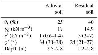
Adapted from Aristizábal (2013) and Aristizábal et al. (2016).

With the infinite slope stability model, FoS for each raster cell is calculated with respect to the bottom of the soil. The analysis with truncated ellipsoidal failure surfaces is performed in a procedure with 1000 simulated surfaces touching each cell. Preliminary tests have indicated that this value represents a good compromise between computational efficiency and accuracy of the results. Each ellipsoidal slip surface is defined by the coordinates of the center and the variable lengths of the three half-axes, the aspect, the inclination and the offset center above the terrain; the failure surfaces include widths between 10 and 100 m and lengths between 10 and 200 m, with a maximum truncated depth of 2.8 m.

Quantitative evaluation of the empirical adequacy of the r.slope.stability model results are accomplished through a confusion matrix and an ROC analysis for the continuous output. Each raster cell of both the observed data (inventory) and the predicted data (model result) is assigned to one of two classes: stable (no landslide mapped or FoS ≥ 1, respectively) or unstable (landslide mapped or FoS < 1, respectively; Fawcett, 2005). The overlay of the classes is known as the confusion matrix, where each raster cell is assigned to one of four classes: true positive (observed unstable cell is predicted as unstable), true negative (observed stable cell is predicted as stable), false positive (observed stable cell is predicted as unstable) and false negative (observed unstable cell is predicted as stable).

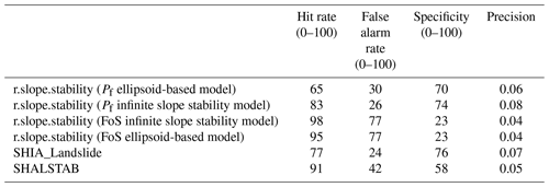
The statistical indexes measuring the performance (Table 4) are the true positive rate or hit rate (TPr), defined as the ratio between the true positives and the observed positives. The true negative rate or specificity (TNr) is the ratio between the true negatives and the observed negatives. The false positive rate or false alarm rate (FPr) is defined as the ratio between the false positives and the observed negatives; the positive predictive value, also called the precision, is the ratio between the true positives and the total predicted positives (Aristizábal et al., 2015, 2016). Evaluation only considers the area covered by the landslide inventory. The ROC analysis plots TPr against FPr for various threshold levels of P_f.

r.slope.stability is compared with the SHALSTAB and SHIA_Landslide models to evaluate the consistency of the results. The SHALSTAB model, developed by Montgomery and Dietrich (1994), applies a topographic index to estimate the saturation of the soil as a function of rainfall infiltration. This procedure builds on the assumption that surface topography can be used as a main indicator of landslide susceptibility (Aristizábal et al., 2015). The model employs the hydrological model TOPOG which uses steady-state rainfall and an infinite slope approach for the geotechnical component (O'Loughlin, 1986). SHIA_Landslide is a physically based and conceptual model, developed by Aristizábal et al. (2016), for computing positive pore pressure changes as well as the resulting changes in FoS due to rainfall infiltration, coupling a distributed hydrological model with a classical infinite slope stability model.

5 Results

The results using the deterministic analysis with the infinite slope stability model in r.slope.stability are shown in Fig. 3a, whereas the results obtained with the slip surface model are shown in Fig. 3b, both of them in terms of FoS. Table 2 shows the confusion matrix calculated by comparing the deterministic analysis results with the scars in the landslide inventory map. For the infinite slope stability model, unstable conditions with FoS < 1 are shown for 79.2 % of the catchment area, whereas only 10.5 % show acceptably stable conditions with FoS values >1.5; these areas correspond to the lower parts of the catchment formed by alluvial sediments with very gentle slopes. With regard to the slip surface model, 84 % of the catchment area show FoS < 1, and only 5.8 % show acceptable stability conditions with FoS > 1.5.

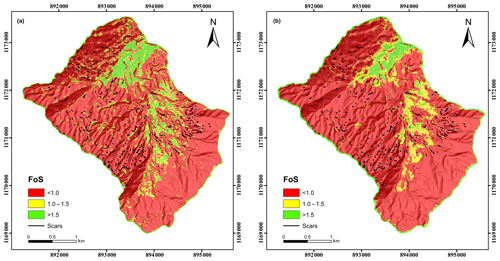
Figure 3 Landslide susceptibility map computed with r.slope.stability. (a) Infinite slope stability model. (b) Ellipsoid-based model.

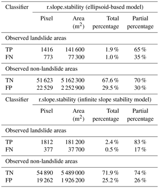
Table 2 The confusion matrix for the deterministic analysis. TP: true positive, FN: false negative, TN: true negative FP: false positive.

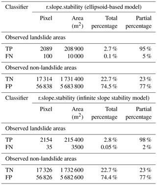
Figure 4 illustrates the results of the probabilistic component of r.slope.stability used with the infinite slope stability model (Fig. 4a) and with the slip surface model (Fig. 4b) in terms of P_f. This probability is computed as the proportion of parameter combinations predicting FoS < 1.0 at a specific raster cell. Table 3 shows the confusion matrix calculated by comparing the probabilistic analysis results with the scars in the landslide inventory map. To define the critical P_f thresholds, the distance to perfect classification parameter (r) proposed by Medina-cetina and Cepeda (2010) is used:

$$\begin{array}{}\text{(3)}& r=\sqrt{(\mathrm{FPr}{)}^{\mathrm{2}}+(\mathrm{1}-\mathrm{TPr}{)}^{\mathrm{2}}}.\end{array}$$

The threshold values yielding the lowest value of r, indicating the best model performance, are used to discriminate between predicted positive and predicted negative cells. We are fully aware that this is a purely statistical optimization approach, not necessarily meaningful from a geotechnical point of view – an issue that will be further elaborated in Sect. 6.

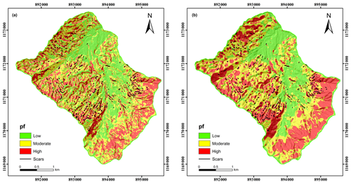
Figure 4 Probability of failure map computed with r.slope.stability. (a) Infinite slope stability model. (b) Ellipsoid-based model.

Table 3 The confusion matrix for the probabilistic analysis.

For the infinite slope stability model a minimum value of r=0.31 is obtained for P_f=0.96, whereas for the slip surface model a minimum value of r=0.46 is obtained for P_f=0.99. For the infinite slope stability model, unstable conditions with P_f>0.96 are shown just for 30.5 % of the catchment area, whereas 69.5 % show stable conditions (FoS ≥ 1.0). 36.4 % of the catchment display values of P_f>0.99 according to the slip surface model, whereas 63.6 % display stable conditions. Unstable hillslopes, according to this criterion, are located mostly in the southern portion of the catchment, where no landslide inventory is available.

According to the confusion matrix, the deterministic analysis of r.slope.stability correctly predicts 98 % and 95 % of the observed landslide areas with the infinite slope stability model and the slip surface model, respectively. The other 2 % and 5 % are predicted as stable but did in reality experience landslides according to the inventory. However, for the observed non-landslide areas, only 23 % are correctly predicted as stable by the infinite slope model and slip surface model, whereas the other 77 %, which are predicted as unstable, did not fail according to the inventory. The deterministic model is more efficient in correctly classifying slopes where landslides occurred and less efficient at classifying slopes on which landslides did not occur. With the thresholds of r applied in this study, the confusion matrix for the probabilistic analysis shows a correct prediction of 83 % and 65 % of the observed landslide areas with the infinite slope stability model and the slip surface model, respectively. The other 17 % and 35 % are erroneously predicted as stable according to the inventory. For the observed non-landslide areas 74 % and 70 % are correctly predicted as stable by the infinite slope model and slip surface model, respectively, whereas only 26 % and 30 % are predicted as unstable, but did not fail.

The values of the area under the ROC curve (AUC) indicate a good ability of the probabilistic results to distinguish between susceptible and less susceptible areas (Fig. 5). The infinite slope stability model yields AUCs of 0.82 and 0.83 for the deterministic and probabilistic analyses, respectively, whereas the slip surface model performs worse, but still fair (0.73 and 0.71).

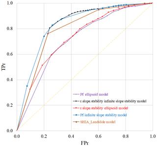
Figure 5 ROC curve models, r.slope.stability (infinite slope stability model) deterministic curve (0.83) and P_f (0.82) for r.slope.stability (ellipsoid-based model) deterministic curve (0.73) and P_f (0.71), SHIA_Landslide model (0.77).

Table 4 summarizes the statistical indices measuring the performance and prediction of the r.slope.stability model compared to SHALSTAB and SHIA_Landslide for the La Arenosa catchment. Figure 5 focuses on the performance of AUC for the r.slope.stability model compared to SHIA_Landslide in the La Arenosa catchment, the better yield corresponds to the infinite slope stability model.

Table 4 Statistical indexes measuring the performance of r.slope.stability and the other models.

Adapted from Aristizábal et al. (2015, 2017).

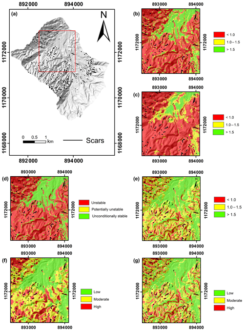
Figure 6 Comparison of results. (a) Analysis area. (b) FoS obtained with r.slope.stability (infinite slope stability model). (c) FoS obtained with r.slope.stability (slip surface model). (d) Analysis with SHALSTAB (Aristizábal et al., 2015). (e) FoS obtained with SHIA_Landslide (Aristizábal et al., 2016). (f) P_f obtained with r.slope.stability (ellipsoid-based model). (g) P_f obtained with r.slope.stability (infinite slope stability model).

Figure 6 compares the results of r.slope.stability with SHALSTAB and SHIA_Landslide for a specific area of the catchment. SHALSTAB shows more areas classified as unconditionally unstable and unstable, displaying similarities to the deterministic analysis of r.slope.stability, whereas SHIA_Landslide and the probabilistic analysis of r.slope.stability tend to show fewer areas with FoS < 1 or with high values of P_f. In summary, the deterministic analysis of the r.slope.stability model shows considerably higher hit rates compared to the probabilistic analysis of r.slope.stability, SHALSTAB and SHIA_Landslide. However, both deterministic analyses of r.slope.stability show the highest false alarm rates. The major reasons for this result – and for the similar patterns yielded with SHIA_Landslide – are most likely an underestimate of the geotechnical stability of the material, the neglect of the effects of vegetation, and/or the overestimate of water saturation. Geotechnical testing is often performed on material which is disturbed in one or the other way, so that the resulting parameters do not necessarily represent natural conditions over larger areas. Roots could lead to some degree of stabilization, and it could also be that vegetation retains sufficient water to avoid full saturation of the soil throughout the catchment.

6 Discussion

In this work, the r.slope.stability tool was applied to the La Arenosa catchment, where the models SHALSTAB and SHIA_Landslide were tested before (Aristizábal et al., 2015, 2016). An ideal model performance simultaneously maximizes TPr and minimizes FPr. In the La Arenosa catchment, the failure area associated with the rainfall event under investigation corresponds just to 2.2 % of the whole catchment. Considering this situation, SHALSTAB tends to predict more unstable areas for this specific rainstorm, increasing the prediction capacity of the model but at the same time increasing the false positive error. Related to this aspect, Cervi et al. (2010) show the limitations of SHALSTAB due to the hydrological assumptions (flow in steady-state conditions). By contrast, the SHIA_Landslide model shows a strong capacity for prediction and a very low FPr. In the case of r.slope.stability, the probabilistic analysis with the infinite slope stability model replicates the 21 September 1990 event with very good reliability, in a much more successful way compared to SHALSTAB and compared to the deterministic r.slope.stability approach, and showing similar performance to that of SHIA_Landslide, with a higher hit rate and a slightly higher value of FPr.

An important advantage of r.slope.stability compared to SHALSTAB and SHIA_Landslide is the possibility of carrying out a probabilistic analysis in terms of considering ranges of the key model parameters. Besides r.slope.stability, there are several physically based models which provide a probabilistic module, such as TRIGRS (Baum et al., 2010) and ALICE (Thiery et al., 2017). Much more work has to be developed in the direction of including probabilistic analysis and improving the predictive capacity of models. Measuring geotechnical and hydraulic parameters for large areas is difficult, time-consuming and expensive, and there is an inherent variability in parameters associated with lithology and soil formation processes (Canli et al., 2017). Similarly, soil thickness shows very high variability and uncertainty. This means there is much uncertainty related to the horizontal and vertical natural variations of soil hydraulic and geotechnical parameters (Christian and Baecher, 2001). In general, soil properties show a pseudo-random pattern rather than a constant value. Additionally, landslides are more complex than their representation in the physically based models adopted, and the geometrical and mechanical parameters that control slope stability are not known with sufficient accuracy (Griffiths et al., 2012; Guzzetti, 2016).

The conventional deterministic approach neglects uncertainties in the slope stability analysis. Although the FoS computation is more likely to identify areas prone to slope failure during a given hydro-meteorological event rather than to predict the exact locations of specific landslides (Baum et al., 2010), FoS is often not a reliable indicator of the slope stability conditions because it is – in terms of interpretation – a binary value derived from several uncertain parameters (Chowdhury et al., 2009). Thus, considering that physically based models are very sensitive to soil properties and soil depth, the probability distribution of failure is a much better indicator of the slope stability conditions.

Probabilistic analyses permit the inclusion of natural soil variations in the analysis, but the mechanism of failure is also fundamental for obtaining adequate results. In the case of the 21 September 1990 rainstorm, the infinite slope stability analysis of the r.slope.stability model using planar shallow failure surfaces shows a better performance than the analysis using an ellipsoidal failure surface. The results obtained show that the failure geometry is most appropriately approximated by shallow planar surfaces, which is confirmed by the reference information: Even though Hermelin et al. (1992) and Garcia (1995) mentioned that both shallow and deep-seated landslides were observed after the studied rainfall event, Velásquez and Mejía (1991) underlined the dominance of shallow landslides. This also agrees with the type of landslides often triggered by short, heavy rainfall events causing a rapid increase in pore pressure (Crosta, 1998). Such landslides are characterized by small and shallow, slope-parallel failure planes (depth of 0.3–2 m; Anderson and Sitar, 1995). The displaced material, by means of processes of static liquefaction and rapid reduction of shear strength in undrained conditions, develops into flows that spread downward (Anderson and Sitar, 1995; Wang and Sassa, 2003). This type of landslide is described by Hungr et al. (2014) as a debris avalanche. In cases where failures occur on slip surfaces with curved shapes, the assumption of ellipsoid-shaped slip surfaces would be expected to provide better results. This indicates the necessity of evaluating a priori the mechanism of failure and then employing the most appropriate model, or – if both mechanisms are relevant – evaluating the model results with different sub-datasets of the inventory. In the present study, due to the lacking distinction of landslide mechanisms in the inventory at the level of individual landslides, we applied both the infinite slope stability model and the slip surface model in order to cover a broad range of mechanisms. The result of the evaluation against the entire landslide inventory was in line with the generally reported dominance of shallow translational landslides.

The current version of r.slope.stability does not permit variation of the saturation level, meaning that the analysis has to be carried out in either dry or saturated conditions. In the r.slope.stability model, including the role of the infiltration process under saturated conditions in particular could strongly improve the model performance in terms of being more effective in considering local hydrological conditions which govern slope instability processes (Mergili et al., 2014a, b), given that the required data are available.

7 Conclusions

In this work, we have presented the results of r.slope.stability for the La Arenosa catchment in the Colombian Andes. r.slope.stability is a 2.5-D slope stability model capable of dealing with shallow and deep-seated landslides triggered by rainfall. The model was evaluated with a set of observed landslides triggered by the 21 September 1990 rainstorm, for which different slope stability models had been previously applied. Considering the probabilistic analyses performed, r.slope.stability shows a high hit rate, suggesting an acceptable prediction capacity for failure areas (65 %–83 %) for the infinite slope stability model and the slip surface model, respectively. The false alarm rate is relatively low for the infinite slope stability model (26 %) and for the slip surface model (30 %). The AUCs yielded by the probabilistic approach are 0.83 for the infinite slope stability model and 0.71 for the slip surface model. These results clearly suggest a higher performance for the assumption of the shallow, planar failure surface (infinite slope stability) model than for the deep-seated slip surface model, a finding which is in line with the physical characteristics of the observed landslides. Despite the generally good model performance, the results were far too conservative compared to the observations, meaning that either (1) the assumption of the saturation patterns was inappropriate; or (2) the geotechnical parameters fed into the model are not representative of the study area. The same challenges were identified for the SHALSTAB model. Future studies shall further elaborate on this issue.

Compared to many other models, r.slope.stability has the advantage that it supports the derivation of a failure probability in terms of considering ranges of the key model parameters, instead of fixed values. Since in any landslide susceptibility analysis it is necessary to consider that soil parameters and their spatial variability are highly uncertain, the computation of failure probabilities in addition to FoS is highly recommended. In Colombia, hazard mapping is mandatory for use land planning in urban areas. Results like the slope failure probability (Fig. 6f and g) are considered suitable for this purpose. However, they only represent one step on the long way to a more reliable landslide susceptibility and hazard mapping.

• i.

  Much of the landslide risk in the Arenosa catchment is not so much related to the failure of unstable slopes, but rather to the downslope propagation of the mobilized material as debris flows (Velásquez and Mejía, 1991). Therefore, coupling of the slope stability model results with mass flow simulation tools is absolutely necessary (Mergili et al., 2017; Bout et al., 2018).

• ii.

  Slope failure probabilities – or impact indicator indices Mergili et al., 2017) – take into account neither the dimension of time nor the fine-scale patterns of the geotechnical characteristics of the catchment. Consequently, those results have to be interpreted in a relative, qualitative sense rather than an absolute, quantitative sense. The combination of these maps with expert judgment is therefore essential to define suitable thresholds separating the study area into different zones with their individual hazard levels and recommendations for action.