Reciprocal Green's functions and the quick forecast of submarine landslide tsunamis

Although tsunamis generated by submarine mass failure are not as common as those induced by submarine earthquakes, sometimes the generated tsunamis are higher than a seismic tsunami in the area close to the tsunami source, and the forecast is much more difficult. In the present study, reciprocal Green's functions (RGFs) are proposed as a useful tool in the forecast of submarine landslide tsunamis. The forcing in the continuity equation due to depth change in a landslide is represented by the temporal derivative of the water depth. After a convolution with reciprocal Green's function, the tsunami waveform can be obtained promptly. Thus, various tsunami scenarios can be considered once a submarine landslide happens, and a useful forecast can be formulated. When a submarine landslide occurs, the various possibilities for tsunami generation can be analyzed and a useful forecast can be devised.

1 Introduction

A tsunami is a serious hazard to coastal cities, and its forecast is essential for hazard mitigation. Of all tsunami hazards, seismic tsunamis are easier to forecast because earthquake information can be retrieved and broadcasted very quickly. For example, approaches used in the broadband seismic network of Taiwan can resolve the rupture plane, rupture type and rupture direction within a few minutes (Hsieh et al., 2014). With the aid of elasticity theories and regression formula for assessing the length scale of fault ruptures, the tsunami source can be estimated with satisfactory accuracy (see, e.g., Chen et al., 2015). Based on Green's functions (GFs; see, e.g., Wei et al., 2003), reciprocal Green's functions (RGFs; see, e.g., Chen et al., 2012) or real-time direct simulation, the propagation of a tsunami is calculated over a short time period. The coastal inundation then can be obtained by real-time direct simulations, analytical solutions (see, e.g., Lin et al., 2014) or pre-calculated inundation maps (see, e.g., Gusman et al., 2014). The RGF approach was integrated, and an economical forecast system was developed to provide both offshore water surface elevation and an inundation map. The efficiency and robustness of these systematic analyses are superior to real-time equation solving, as has been shown in previous studies (Chen et al., 2015).

Besides seismic tsunamis, a few recent events are believed to be closely related to submarine mass failure (SMF). For example, the 1998 Papua New Guinea tsunami (Tappin et al., 2001), the 2007 Chilean tsunami (Sepúlveda et al., 2010) and the 2018 Sulawesi tsunami (Heidarzadeh et al., 2018) all occurred after submarine earthquakes. In each case the earthquake was not strong enough to generate a big tsunami. The devastating tsunamis following the earthquake were all attributed to submarine landslides triggered by the earthquake.

Besides these recent events, some historical events are also believed to be the result of submarine mass failure (SMF). The mysterious tsunami that struck the southwestern coast of Taiwan (Li et al., 2015), which will be simulated later, is used as an example in the present study.

Although the RGF approach is quick and economical, extending this approach from seismic tsunamis to SMF tsunamis is not straightforward. Fault rupture in an earthquake is much faster than the water wave speed, and hence the rupture process can be simply represented by initial sea surface elevations which are determined by sea bottom deformation after the fault rupture. Thus, only the response to the initial water level is needed. On the other hand, an SMF forces the sea water and continuously contributes to the formation of a tsunami; a much more complicated computation is involved.

As SMF tsunamis are devastating to coastal areas, their forecast and associated hazard mitigation are very important. However, no available technology can provide accurate information on the details of the SMF. The location, depth, volume, density, directional movement, movement speed, distance and duration of the slide displacement are difficult to determine accurately. As the RGF approach is fast and robust, different SMF parameters and locations can be considered very quickly. Thus, ensemble forecasting of SMF tsunamis becomes possible and can be used for tsunami hazard mitigation.

2 Methodology

A tsunami is a long wave and can be properly described by the shallow-water equations (SWEs):

$$\begin{array}{}\text{(1)}& \begin{array}{rl}& {\displaystyle \frac{\partial }{\partial t}}\mathit{\eta }+{\displaystyle \frac{\partial }{\partial x}}P+{\displaystyle \frac{\partial }{\partial y}}Q=\mathrm{0},\\ & {\displaystyle \frac{\partial }{\partial t}}P+gd{\displaystyle \frac{\partial }{\partial x}}\mathit{\eta }=\mathrm{0},\\ & {\displaystyle \frac{\partial }{\partial t}}Q+gd{\displaystyle \frac{\partial }{\partial y}}\mathit{\eta }=\mathrm{0},\end{array}\end{array}$$

where η is the free surface elevation, P and Q are volume fluxes along the x and y directions, t is time, g is the gravitational acceleration, and d is the water depth taken from the real bathymetry. In the present study, two equation sets will be presented: (1) the SWEs with SMF forcing and (2) the SWEs with impulsive forcing represented by a δ function. With the aid of an integral transform, the complete solution to the SWEs is a convolution of the forcing and the GF. The detailed mathematics and its physical meaning will be presented in this section.

Because of the reciprocity between the GF and RGF, the SMF tsunami can be obtained as the convolution of the slide forcing and the RGF. This convolution approach with the RGF is then applied to a few idealized SMF scenarios, and the results are compared in the next section with direct simulation using the Cornell multi-grid coupled tsunami model (COMCOT; Wang and Power, 2011). These comparisons are used to verify the RGF-convolution approach in calculating SMF tsunamis.

2.1 Green's functions for shallow-water equations

GFs are responses of a system to an impulsive point forcing. For a homogeneous medium with an infinite domain, GFs can be obtained analytically. The distribution of analytic GFs for various differential equations can be obtained from boundary conditions by numerical approaches such as the boundary element method (see, e.g., Brebbia et al., 1984).

Another type of GF includes both the inhomogeneity and the boundary conditions. In this case, an analytic solution is usually not available and each GF has to be solved by numerical codes like COMCOT. Numerical GFs have previously been applied in seismic tsunami forecast (e.g., Wei et al., 2003). This kind of forecast can be completed over a very short time period if the GFs are pre-calculated. There will be no need for equation solving, and the forecast is simply a summation over the product of the initial sea surface elevations and the corresponding GFs.

The physical meaning of the GF for SWEs is explained as follows. By definition volume flux is the integration of a velocity component from the sea bottom to the water surface and equals the average velocity multiplied by the undisturbed water depth d if the vertical distribution of horizontal velocity is uniform. The volume flux vector and horizontal gradient operator are defined for brevity as

$$\mathit{V}=\left(P,Q\right),$$

and

$${\mathrm{\nabla }}_H=\left({\displaystyle \frac{\partial }{\partial x}},{\displaystyle \frac{\partial }{\partial y}}\right).$$

If an impulsive forcing (δ function) is added on the right-hand side of the continuity equation, SWEs shown in Eq. (1) become

$$\begin{array}{}\text{(2)}& \begin{array}{rl}& {\displaystyle \frac{\partial }{\partial t}}\mathit{\eta }+{\mathrm{\nabla }}_H\cdot \mathit{V}=\mathit{\delta }\left(t\right)\mathit{\delta }(x-x_{\mathrm{s}})\mathit{\delta }(y-y_{\mathrm{s}}),\\ & {\displaystyle \frac{\partial }{\partial t}}\mathit{V}+gd{\mathrm{\nabla }}_H\mathit{\eta }=\mathrm{0},\end{array}\end{array}$$

where (x_s, y_s) is the location of the source point. Integrating the continuity equation over an infinitesimal space domain Ω and a short period of time gives

$$\begin{array}{rl}\underset{{\mathrm{0}}^{-}}{\overset{{\mathrm{0}}^{+}}{\int }}& \mathrm{d}t\underset{\mathrm{\Omega }}{\int }{\displaystyle \frac{\partial }{\partial t}}\mathit{\eta }+{\mathrm{\nabla }}_H\cdot \mathit{V}\mathrm{d}x\mathrm{d}y\\ & =\underset{{\mathrm{0}}^{-}}{\overset{{\mathrm{0}}^{+}}{\int }}\underset{\mathrm{\Omega }}{\int }\mathit{\delta }\left(t\right)\mathit{\delta }(x-x_{\mathrm{s}})\mathit{\delta }(y-y_{\mathrm{s}})\mathrm{d}x\mathrm{d}y\mathrm{d}t=\mathrm{1}.\end{array}$$

The second term on the left-hand side is negligible if the domain Ω is small, and the continuity equation can be simplified to

$$\begin{array}{}\text{(3)}& {\left.\underset{\mathrm{\Omega }}{\int }\mathit{\eta }\mathrm{d}x\mathrm{d}y\right|}_{t={\mathrm{0}}^{+}}-{\left.\underset{\mathrm{\Omega }}{\int }\mathit{\eta }\mathrm{d}x\mathrm{d}y\right|}_{t={\mathrm{0}}^{-}}=\mathrm{1}.\end{array}$$

That is, the initially elevated volume at t=0 equals 1. The GF is the response due to an impulsive unit volume increase in η at the source point ${\mathit{r}}_{\mathrm{s}}=(x_{\mathrm{s}},y_{\mathrm{s}})$. This response is denoted as a vector G_η:

$${\mathit{G}}_{\mathit{\eta }}(\mathit{r},t;{\mathit{r}}_{\mathrm{s}})\equiv 〈\mathit{\eta }\mathit{\eta },\mathit{P}\mathit{\eta },\mathit{Q}\mathit{\eta }〉,$$

where ηη is the η response, Pη is the response of the variable P and Qη is the response of Q to the impulsive η increase. Thus, the SWEs for a GF can be rewritten as

$$\begin{array}{}\text{(4)}& \begin{array}{rl}& {\displaystyle \frac{\partial }{\partial t}}\mathit{\eta }\mathit{\eta }+{\displaystyle \frac{\partial }{\partial x}}\mathit{P}\mathit{\eta }+{\displaystyle \frac{\partial }{\partial y}}\mathit{Q}\mathit{\eta }=\mathit{\delta }\left(t\right)\mathit{\delta }(x-x_{\mathrm{s}})\mathit{\delta }(y-y_{\mathrm{s}}),\\ & {\displaystyle \frac{\partial }{\partial t}}\mathit{P}\mathit{\eta }+gd{\displaystyle \frac{\partial }{\partial x}}\mathit{\eta }\mathit{\eta }=\mathrm{0},\\ & {\displaystyle \frac{\partial }{\partial t}}\mathit{Q}\mathit{\eta }+gd{\displaystyle \frac{\partial }{\partial y}}\mathit{\eta }\mathit{\eta }=\mathrm{0}.\end{array}\end{array}$$

It should be noted that in a discretized numerical simulation, a unit elevation is used as the initial impulse. Hence, the impulsive volume increase for a numerical GF is the area of the source grid instead of 1.

A briefer expression for Eq. (4) can be obtained by introducing the operator

$$\begin{array}{}\text{(5)}& O\equiv \left[\begin{array}{lll}\mathrm{0}& \frac{\partial }{\partial x}& \frac{\partial }{\partial y}\\ gd\frac{\partial }{\partial x}& \mathrm{0}& \mathrm{0}\\ gd\frac{\partial }{\partial y}& \mathrm{0}& \mathrm{0}.\end{array}\right].\end{array}$$

After expressing the forcing δ function as a vector with three components corresponding to the three equations of Eq. (4),

$$\begin{array}{}\text{(6)}& {\mathit{\delta }}_{\mathit{\eta }}\left({\mathit{r}}_{\mathrm{s}}\right)\equiv 〈\mathit{\delta }\left(t\right)\mathit{\delta }(x-x_{\mathrm{s}})\mathit{\delta }(y-y_{\mathrm{s}}),\mathrm{0},\mathrm{0}〉,\end{array}$$

the SWEs for the GF can be simplified to

$$\begin{array}{}\text{(7)}& {\displaystyle \frac{\partial }{\partial t}}{G}_{\mathit{\eta }}^{\mathrm{T}}=-O{G}_{\mathit{\eta }}^{\mathrm{T}}+{\mathit{\delta }}_{\mathit{\eta }}^{\mathrm{T}}.\end{array}$$

Note that the superscript T represents the transpose of a vector.

2.2 SMF tsunami

If the sea bottom is deformable and the characteristic lengths of the source area are much larger than the depth, the continuity equation in SWEs should include a new source term $-\partial \mathrm{d}/\partial t$, the temporal variation in the sea depth (Løvholt et al., 2015). On the other hand, if the thickness of the slide is much smaller than the total water depth, the contribution of the SMF in the momentum equations is negligible. Thus, the process of tsunami generation can be described by the following matrix equation (Lynett and Liu, 2002; Wang and Liu, 2006):

$$\begin{array}{}\text{(8)}& {\displaystyle \frac{\partial }{\partial t}}\left[\begin{array}{l}\mathit{\eta }\\ P\\ Q\end{array}\right]=-\left[\begin{array}{lll}\mathrm{0}& \frac{\partial }{\partial x}& \frac{\partial }{\partial y}\\ gd\frac{\partial }{\partial x}& \mathrm{0}& \mathrm{0}\\ gd\frac{\partial }{\partial y}& \mathrm{0}& \mathrm{0}\end{array}\right]\left[\begin{array}{l}\mathit{\eta }\\ P\\ Q\end{array}\right]+\left[\begin{array}{l}-\frac{\partial d}{\partial t}\\ \mathrm{0}\\ \mathrm{0}\end{array}\right].\end{array}$$

Note that the same governing equations are used in the most recent version of the COMCOT (Wang and Power, 2011). With this formulation, tsunami generation is related to the temporal variation in the sea depth. Thus, the SMF continuously contributes to the tsunami. Following the notation of the previous section, when we introduce an unknown vector,

$$\begin{array}{}\text{(9)}& \mathit{Z}\equiv 〈\mathit{\eta },P,Q〉,\end{array}$$

and a forcing vector,

$$\begin{array}{}\text{(10)}& \mathit{f}\equiv 〈-{\displaystyle \frac{\partial d}{\partial t}},\mathrm{0},\mathrm{0}〉,\end{array}$$

the SWEs governing the generation and propagation of an SMF tsunami then can be expressed in a brief way:

$$\begin{array}{}\text{(11)}& {\displaystyle \frac{\partial }{\partial t}}{\mathit{Z}}^{\mathrm{T}}=-\mathit{O}{\mathit{Z}}^{\mathrm{T}}+{\mathit{f}}^{\mathrm{T}}.\end{array}$$

Similar to Eq. (7), the superscript T represents the transpose of a vector.

2.3 GF and the quick forecast of SMF tsunamis

Similarities between the SWEs of GFs in Eqs. (7) and (11) for SMF tsunamis are obvious. For both equations, the left-hand sides are identical. The right-hand side for the GF is a δ function, while that for the SMF tsunami is the temporal variation in the sea depth, which represents the forcing due to sliding. Applying a Laplace transform, the problem for SMF tsunamis can be solved as the convolution of the GF and the forcing as

$$\begin{array}{}\text{(12)}& \begin{array}{rl}& \mathit{Z}={\mathit{G}}_{\mathit{\eta }}*{\mathit{f}}^T\\ & =\underset{\mathrm{0}}{\overset{t}{\int }}\int \underset{{\mathrm{\Omega }}_S}{\int }{\mathit{G}}_{\mathit{\eta }}({\mathit{r}}_{\mathrm{s}},\mathit{\tau };\mathit{r})\cdot {\mathit{f}}^T({\mathit{r}}_{\mathrm{s}},t-\mathit{\tau })\mathrm{d}{\mathrm{\Omega }}_S\mathrm{d}\mathit{\tau }\\ & \mathrm{or}\\ & \mathit{\eta }=\underset{\mathrm{0}}{\overset{t}{\int }}\int \underset{{\mathrm{\Omega }}_S}{\int }-{\displaystyle \frac{\partial \mathrm{d}}{\partial t}}({\mathit{r}}_{\mathrm{s}},t-\mathit{\tau })\mathit{\eta }\mathit{\eta }({\mathit{r}}_{\mathrm{s}},\mathit{\tau };\mathit{r})\mathrm{d}{\mathrm{\Omega }}_S\mathrm{d}\mathit{\tau }\end{array}\end{array}$$

Thus, the continuous contribution of the slide can be represented by a convolution.

Besides the convolution, another term will be added if the initial condition is nontrivial. This contribution from the initial sea surface elevation or initial flow is consistent with the elevation GF solution for seismic tsunamis (see, e.g., Chen et al., 2015), which is generated by impulsive fault rupture and can be constructed as a linear combination of GFs. However, if the tsunami calculation starts from the resting state and the initial state is set before the onset of landslide, neither initial flow nor initial elevation exists. Hence, the contribution due to initial conditions vanishes and Eq. (12) can completely describe the SMF tsunami.

2.4 Reciprocity of Green's functions

Applying the reciprocity of the GF and RGF in the forecast of tsunamis was first suggested by Loomis (1979). The first tsunami forecast system that applies the reciprocity of the GF and RGF was shown in Chen et al. (2015), which is designed specifically for seismic tsunamis.

The elevation response to an initial impulsive elevation (GF) and its reciprocal (RGF) with the locations of source and receiver exchanged are calculated. The reciprocity between these two in SWEs can be verified numerically. The comparison of these two results is shown to be identical, as has been shown in Chen and Liu (2009) and Chen et al. (2012, 2015).

Using the RGF instead of the GF is done to reduce the computer time in computing the pre-calculated GF. For a large source area there will be many GFs which correspond to the forcing at all source points. Pre-calculation of all the GFs is very time-consuming. For the 2011 Tōhoku tsunami, for example, the source zone is approximately 500 km long and 200 km wide. A reasonable 2 min resolution means that 10 000 GFs have to be calculated, and the number of GFs increases if more tsunami source locations are to be considered.

For SMF tsunamis, the source zone is not that large. Still the number of possible submarine sliding sites could be more than 1, and the total number of GFs is large. As the calculations of the GF and RGF are exactly the same except for the initial conditions, using the RGF instead of the GF is much more economical and feasible.

As the length scale of both the GF and RGF is small, it may be wondered if the associated wavelength is not much longer than the water depth and if the dispersion effect should be included. Here the applicability of the GF and RGF in a shallow-water system will be briefly discussed. The length scale is used to determine the order of magnitude for every physical quantity governing the movement of the ocean. By assuming very large horizontal length scales, nonhydrostatic dispersion can be shown to be negligible, and Navier–Stokes equations can be simplified to SWEs. Therefore, by applying SWEs, only the dynamics in an ocean which has no nonhydrostatic dispersion is the focus. A GF and RGF of SWEs is the response of this non-dispersive ocean due to an initially elevated concentrated volume, without recourse to how a real ocean will respond to it. Since the GF and RGF of SWEs can be used to construct the complete solution like Eq. (12), it is a useful mathematical tool in the present study. The dispersion effect is not considered in the present study because including the dispersion of the GF and RGF will not improve the tsunami solution in any way.

A similar question on the length scale is also frequently encountered in solving SWEs by the finite difference or other numerical schemes. The grid size in discretizing the SWEs is also a length scale, but it is not necessary that each grid be much longer than the water depth. A shorter grid size does not imply that the length scale assumption for SWEs is violated because the focus is only on the dynamics in a non-dispersive ocean. Thus, the finite difference and other numerical schemes are also useful mathematical tools in solving SWEs. In fact, if a grid size much larger than the water depth is insisted on, then a solution of acceptable accuracy can never be obtained.

3 Results

In this section, three idealized SMF cases are used to verify the RGF approach. The first two cases are vertical sea bottom movements with different displacement rates. The third case is a historical event following Li et al. (2015), with an idealized truncated hyperbolic slide whose kinematics is described in Enet and Grilli (2007). In each case, direct COMCOT simulation is compared with an RGF approach and the results agree well with each other. Thus, using the RGF with convolution is a fast and accurate substitute for the simulation of SMF tsunamis.

3.1 Fast and slow sea bottom movements

In the first two cases, simple sea bottom movements are considered. Both the direct COMCOT simulation for the SMF tsunami and the RGF calculation are done over the area 21.2–23.2^∘ N, 119.0–121.1^∘ E, as shown in Fig. 1. The spatial resolution is 0.06 min, and both simulations last 40 min. Case 1 considers a fast bottom movement. The area enclosed by the red rectangle to the southwest of Taiwan in Fig. 1 is set to move 3 m downward in 120 s. This downward movement occurs uniformly in both space and time. The whole rectangular area subsides at a velocity of −0.025 m s⁻¹ for 120 s.

Figure 1 The simulation domain for Cases 1 and 2: 21.2–23.2^∘ N, 119.0–121.1^∘ E, with the source zone denoted by the red rectangle to the southwest of Taiwan. The locations of the two coastal cities Anping (AP) and Kaohsiung (KH) are also provided where initial impulses are applied to calculate RGFs.

On the southwestern coast of Taiwan, Anping (AP) and Kaohsiung (KH) are the two largest cities. The locations of AP and KH are shown in Fig. 1, and the exact locations for the forecast of these two vulnerable cities are respectively 22.940^∘ N, 120.088^∘ E, and 22.590^∘ N, 120.250^∘ E. For the calculation of the RGF, initially the sea surface elevation at either AP or KH is set to be 1 m. The evolution of the sea surface over the whole domain following the initial impulse is the desired RGF.

The direct COMCOT gives the time series of the sea surface represented by the red line in Fig. 2, and the convolution of the RGF and the constant −0.025 m s⁻¹ over the red rectangle area from 0 to 120 s gives the blue line. The agreement between these two approaches verifies the theory of this study.

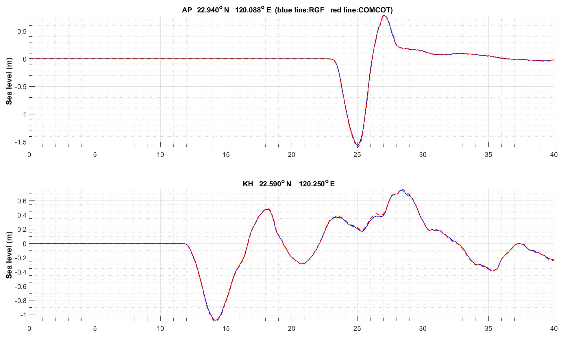
Figure 2 The simulated sea surface time series by direct COMCOT simulation (red) and the RGF approach (blue) of Case 1 for two cities, AP and KH, on the southwestern coast of Taiwan, with locations given in Fig. 1.

Case 2 considers the slow sea bottom change: the area enclosed by the red rectangle to the southwest of Taiwan in Fig. 1 is set to move 3 m downward in 600 s. This downward movement is equivalent to a source strength of −0.005 m s⁻¹, which is uniform in both space and in the 600 s time extension. Comparison between the direct COMCOT simulation and the convolution of the RGF and the constant source strength over the red rectangle area in the 600 s sliding period also gives good agreement, as shown in Fig. 3.

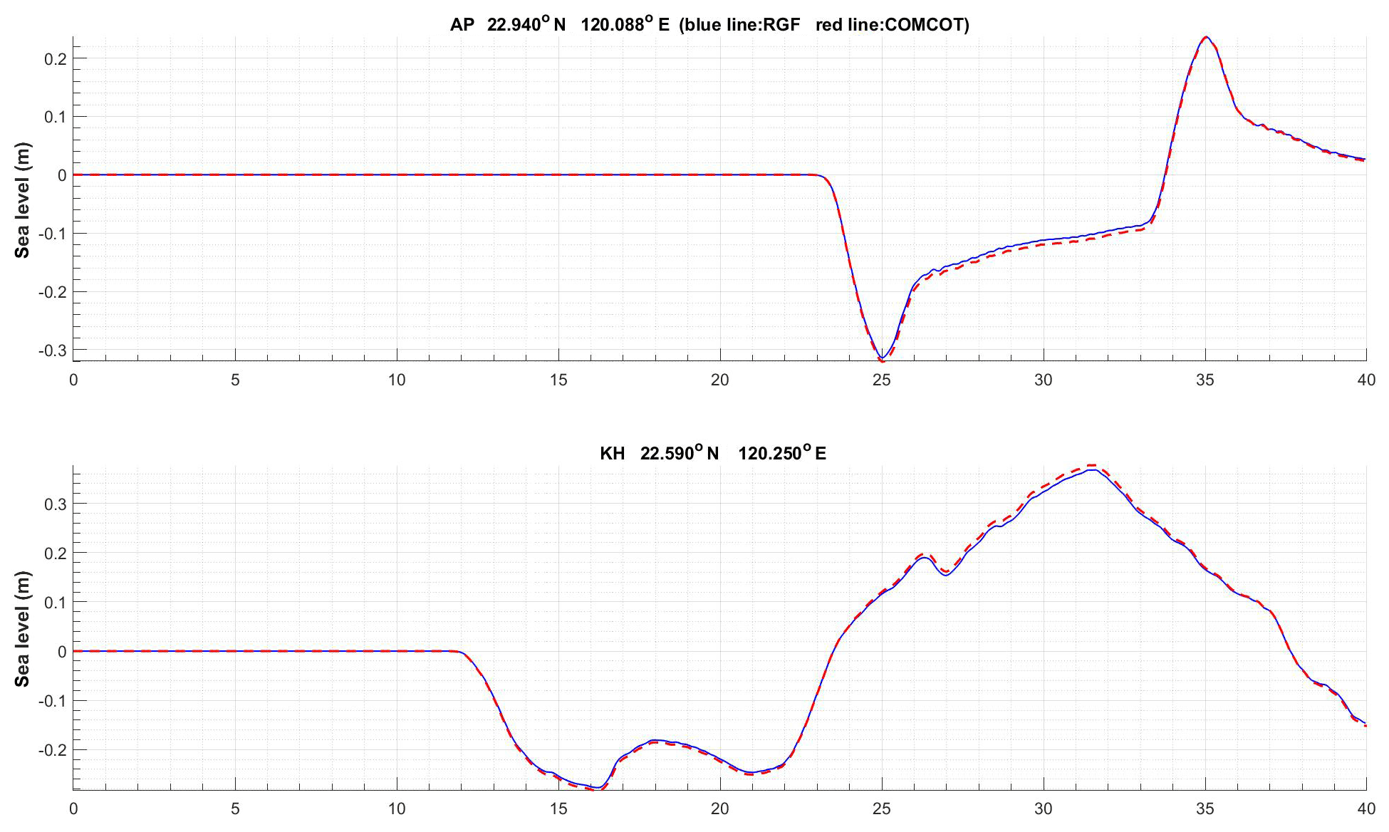
Figure 3 Comparison between the direct COMCOT simulation (red) and the RGF approach (blue) of Case 2 for two cities, AP and KH, on the southwestern coast of Taiwan, with locations given in Fig. 1.

3.2 A historical SMF tsunami on the southwestern coast of Taiwan

For the southwestern coast of Taiwan, a tsunami was reported in the year 1781. The record shows that when the fishers came back after fishing, “they found the houses were submerged and the fishing rafts could sail over the bamboo.” The fishing rafts went out to sea before the tsunami came; therefore, it was a fair day, and hence this flooding is due to a tsunami, not a disguised storm surge. Li et al. (2015) called this event a mysterious tsunami because no big earthquakes had been reported and proposed the devastating tsunami of 1781 to be an SMF tsunami.

Previous studies have shown that both the volume and the cross-sectional area of the slide play an important role in tsunami generation (Lo and Liu, 2017). The deformation of the slide does not significantly change the generated tsunami, and scenarios generated by a rigid slide body can provide the first-order estimate of tsunami wave magnitude (Grilli et al., 2015; Løvholt et al., 2015). Therefore, an idealized model with a rigid slide body is adopted as the third case in the present study. Following Enet and Grilli (2007), the shape of the slide is assumed to be truncated hyperbolic, and the landslide is expressed as

$$z={\displaystyle \frac{T}{\mathrm{1}-\mathit{ϵ}}}\left[\mathrm{sech}\left(k_{b}x\right)\mathrm{sech}\left(k_{w}y\right)-\mathit{ϵ}\right],$$

where T is the maximum thickness,

$$\begin{array}{c}{\displaystyle }{k}_b={\displaystyle \frac{\mathrm{2}}{b}}a\cos h\left({\displaystyle \frac{\mathrm{1}}{\mathit{ϵ}}}\right),\\ {\displaystyle }{k}_w={\displaystyle \frac{\mathrm{2}}{w}}a\cos h\left({\displaystyle \frac{\mathrm{1}}{\mathit{ϵ}}}\right),\end{array}$$

where b and w are the longitudinal and transverse length scales of the slide, and the truncation parameter ϵ is set to be 0.717. Longitudinal and transverse length scales, along with other slide parameters shown in Table 1, have been adopted in Li et al. (2015) and are also used in Case 3 to simulate this historical event in Taiwan. Note that the initial acceleration is the most important SMF parameter that determines the initial elevation of the tsunami if the SMF has a characteristic length much larger than the depth (Løvholt et al., 2015). Hence, the initial acceleration 1.54 m s⁻² obtained by Li et al. (2015) is adopted.

Table 1 The SMF information to the southwest of Taiwan used in the tsunami simulation of Case 3.

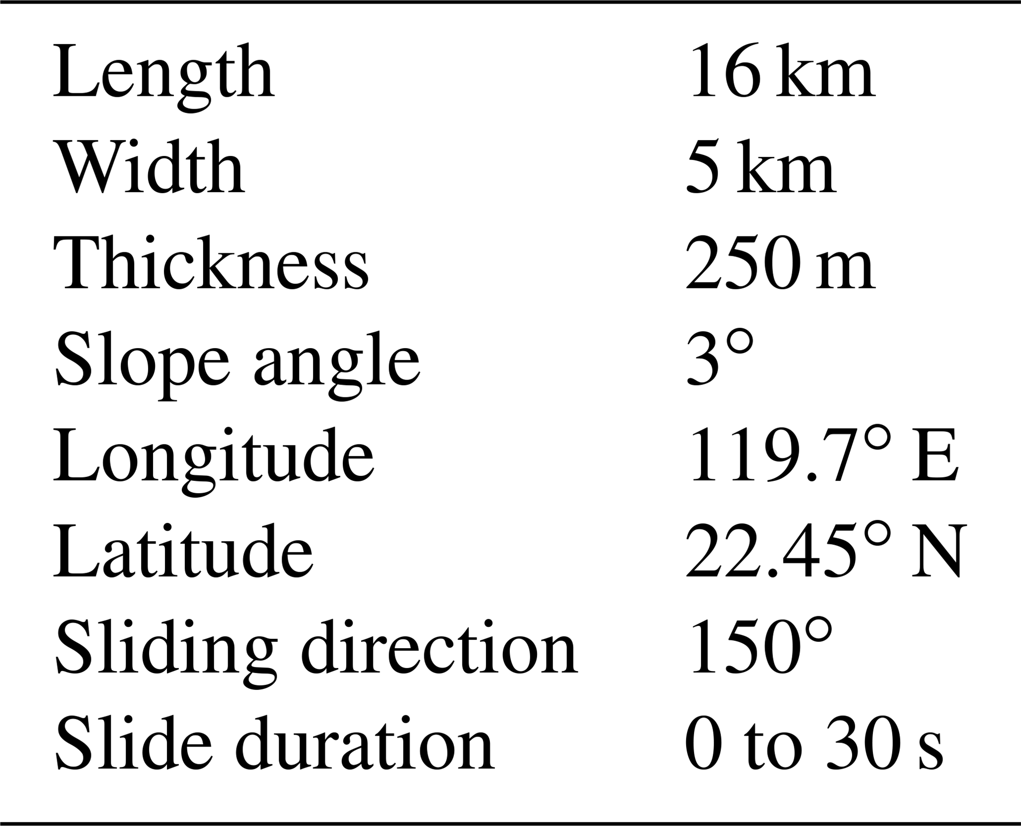
The movement is described by semi-empirical kinematic formulas provided in Enet and Grilli (2007). For example, the slide displacement of the SMF, s(t), is given as

$$s\left(t\right)=s_{\mathrm{0}}\ln \left[\cos h\left({\displaystyle \frac{t}{t_{\mathrm{0}}}}\right)\right].$$

Here t=0 is the time of the slide start and θ is the angle between the slide motion and the horizon. The characteristic length and time of the landslide motion are

$$s_{\mathrm{0}}={\displaystyle \frac{u_t^{\mathrm{2}}}{a_{\mathrm{0}}}},$$

and

$$t_{\mathrm{0}}={\displaystyle \frac{u_t}{a_{\mathrm{0}}}},$$

where the terminal speed u_t is set to be 83.1 m s⁻¹, following Li et al. (2015). The displacement s(t) is explicitly plotted in Fig. 4a based on SMF parameters of Table 1. The displacement s(t) is explicitly plotted in Fig. 4a based on SMF parameters of Table 1. Following Li et al. (2015), the SMF occurs at 22.45^∘ N, 119.7^∘ E, where the water depth is approximately 1100 m. Similar to Cases 1 and 2, the direct COMCOT simulation for the SMF tsunami is done over the area 21.2–23.2^∘ N, 119.0–121.1^∘ E, with 0.06 min spatial resolution. Both the COMCOT and RGF calculations simulate the sea surface evolution for 40 min. Two RGFs exactly the same as those used in Cases 1 and 2 are applied to compute the incident tsunami at two cities, AP and KH, on the southwestern coast of Taiwan.

As shown in Fig. 4b, for the first few waves the water level time series given by direct COMCOT simulation is very close to that of the RGF approach. After the first few waves, the RGF approach and the direct simulation in AP still agree quite well. However, in KH water levels obtained by these two approaches start to separate when t=20 min. The accuracy of the RGF approach is good for forecast purposes, but the discrepancy suggests that some limitations may apply in a big tsunami. More discussions will be given in Sect. 4.4.

4 Discussions and conclusion

4.1 Computer time comparison and its implication

Besides accuracy, the efficiency of the RGF method is compared with the direct simulation. Both the direct simulation and the RGF are calculated with the same 0.06 min resolution, 0.25 s time step and 10⁻¹³ precision. For the same desktop PCs, with 16 GB RAM and Intel i7-9600 CPU, the CPU time for the RGF approach is about 4.2 s, while a direct COMCOT simulation takes 77 min. As the results of both approaches are identical, the RGF is much more economical than the direct COMCOT simulation.

It should be noted a similar simulation with coarser (0.3 min) resolution and a 40 min time extension takes only 39 s for direct simulation, while the RGF approach for the same grid size takes about 2 s. That is, the finer the computation domain, the more economical the RGF approach will be.

The RGF approach is economical, fast and robust because the RGF is pre-calculated and no equation solving is involved. The tsunami waveform can be obtained in 5 s once a submarine landslide is detected. Thus, a tsunami warning can be issued promptly to mitigate possible hazards, with a similar process for a seismic tsunami when an earthquake occurs (see, e.g., Chen et al., 2015).

One problem in the mitigation of SMF tsunamis is that the detection technology of SMF is not as mature and comprehensive as that for earthquakes. Earthquakes are serious hazards; advanced technology has been developed, and most earthquake-prone areas have been covered by seismometer networks. Consequently, seismic information usually can be obtained promptly with very high accuracy, while there is usually no access to information on landslides, especially SMFs.

However, the quick forecast of SMF tsunamis is still possible. For a detailed simulation of the SMF tsunami, information on the volume, density and cohesive property of the slide material and the location, depth, movement speed, distance and duration of the slide displacement are all needed. Some properties such as density and cohesiveness can be measured beforehand in a survey on coastal seas. Besides this, previous studies have shown that both inland and submarine landslides can be detected by hydrophones (e.g., Caplan-Auerbach et al., 2001) or broadband seismometers (e.g., Lin et al., 2010). Thus, it is possible to determine the time and location of the landslide. With idealized models such as that of Enet and Grilli (2007), which was used in this study, as well as information on local bathymetry, the SMF tsunami can be forecast.

Available landslide information is much less accurate than the earthquake information used in existing forecast systems for seismic tsunamis. Instead of giving one single forecast for a seismic tsunami based on one set of fault parameters, a forecast for SMF tsunamis should consider the possibility of different SMF parameters and locations. After calculating all possible parameters, a range of tsunami heights and their arrival time can be released. Hence it can be concluded that a forecast system can be constructed using the RGF. Once a submarine landslide is detected, the range of volume, location, movement speed and other slide information can be estimated. Along with previous knowledge on the local bathymetry and properties of sea bottom sediment, reasonable estimations of the best and the worst (in terms of the devastation induced by the tsunami) situations can be calculated in minutes. Further forecasts such as inundation maps can be generated based on the highest tsunami wave height (Chen et al., 2015). Thus, quick forecasting of SMF tsunamis is possible and can be used for tsunami hazard mitigation.

4.2 Dispersion effect in an SMF tsunami

An SMF usually has a smaller horizontal length scale than the rupture length scale of a tsunamigenic earthquake. The wavelength of an SMF tsunami thus is not as long as a seismic tsunami. It is natural to ask if dispersion may play an important role in an SMF tsunami, and the applicability of the non-dispersive SWEs on an SMF tsunami should be discussed.

Although an SMF tsunami is shorter than a seismic tsunami, the dispersion is not significant because the generated wave also has long wavelengths. Take Case 3 of this study as an example, which corresponds to a historical tsunami to the southwest of Taiwan in 1781. The sea surface waveform generated when the SMF ends is shown in Fig. 5, where the distance between the crest and trough of the tsunami wave is approximately 5 km, and hence the wavelength (10 km) is much larger than the 1.1 km water depth at the SMF site. Since an SMF is usually not far from the shoreline, and the water depth becomes shallower and shallower as the tsunami propagates toward the coast, the wave deformation due to dispersion is limited during its propagation to the coast.

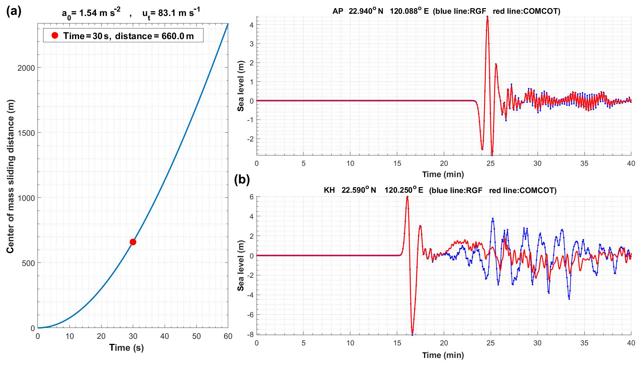
Figure 4 (a) Movement of the 1781 SMF described by semi-empirical kinematic formulas of Enet and Grilli (2007). (b) Comparison between the direct COMCOT simulation (red) and the RGF approach (blue) of Case 3 for two cities, AP and KH, on the southwestern coast of Taiwan, with locations given in Fig. 1.

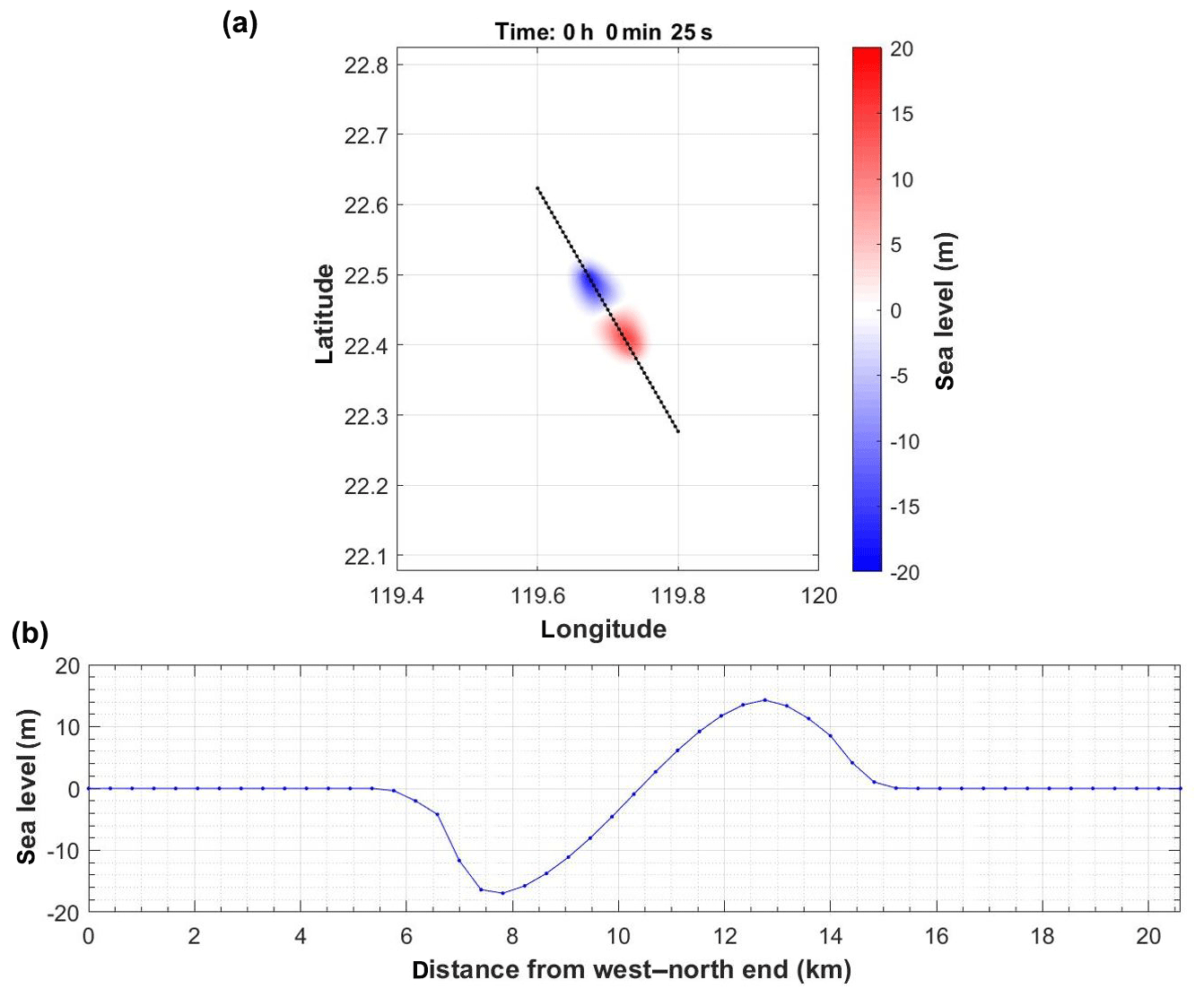
Figure 5 Sea surface waveform when the SMF of Case 3 ends. Panel (a) is the top view, while panel (b) is the cross section along the black dashed line.

In previous studies such as Kilinc et al. (2009) more detailed results have been given and a more comprehensive comparison on waveform and wave height is executed. The waveform simulated in a dispersive model is very similar to the result of a non-dispersive model. Thus, based on the SMF tsunamis discussed above, it can be concluded that the dispersion effect does not significantly change an SMF tsunami. Thus, an SMF tsunami can be simulated by non-dispersive SWEs.

It should be noted that the purpose of this paper is to forecast an SMF tsunami. The dispersion tends to spread different wave components of the tsunami wave; thus, the predicted tsunami waveform may not be very accurate. However, as the information on an SMF is usually very limited, it is not possible to simulate or forecast the tsunami in detail. Compared to the uncertainty of SMFs, waveform discrepancies due to a dispersion effect are minor and negligible, as has been demonstrated in this discussion. Thus, maximum sea surface elevation can be forecast by SWEs and a simple SMF model generated with satisfactory accuracy, and SWEs used in the present study are appropriate choices.

4.3 Convergence of the simulation of SMF tsunamis

To make sure the comparison of the present RGF approach with the direct COMCOT simulation is not meaningless, the simulation should be accurate and a discussion on its convergence is necessary. The truncation error of the modified leap-frog scheme used in COMCOT is of O(Δt) in time and of O(Δx², Δy²) in space. The time step Δt is determined by the Courant–Friedrichs–Lewy condition (see, e.g., Wang and Power, 2011). Hence, the dimension of the grid cell determines the convergence of a tsunami simulation.

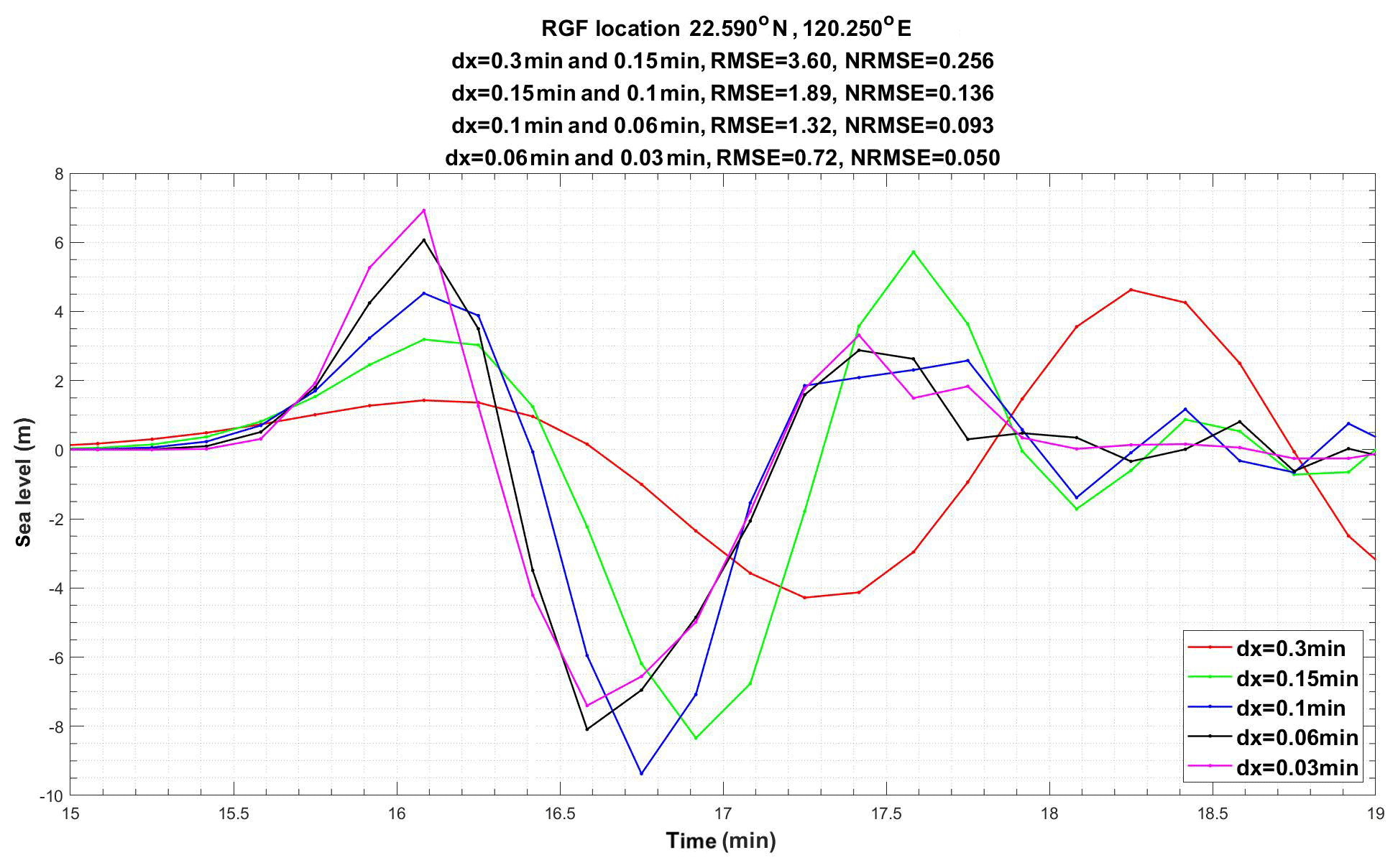
Figure 6 The sea surface due to the historical tsunami of Case 3 in Kaohsiung (KH) simulated with various grid spacings. The RMSE and the NRMSE of each pair of successive grid resolutions are calculated at the top of the figure.

Take Case 3 of this study as an example, which corresponds to a historical tsunami to the southwest of Taiwan in 1781. To test the convergence of the modified leap-frog scheme in SMF tsunamis, the historical tsunami of Case 3 is simulated with various grid spacings. Usually there are at least 10 grids points in a characteristic length to properly describe a flow field. As the width of the slide is 5 km, the maximum allowable grid spacing is 0.3 min, which has been employed in Li et al. (2015). Besides the 0.3 min resolution, grid cells of 0.1, 0.06 and 0.03 min are employed. Based on these simulations, the time series of the water surface at KH are obtained for each kind of resolution, as is shown in Fig. 6. The root-mean-quare error (RMSE) of each pair of successive grid resolutions are calculated. Then, the normalized root-mean-square error (NRMSE), which is the RMSE divided by the maximum wave height, is used to determine the convergence. Both the RMSE and NRMSE are shown at the top of Fig. 6.

For tsunamis, a 10 % NRMSE is a reasonable criterion because many other factors may cause uncertainty much larger than this. As is shown in Fig. 6, the NRMSE between the simulations of 0.1 and 0.06 min is slightly below 10 %, and that between the simulations of 0.06 and 0.03 min is below 6 %. To be on the safe side, the 0.06 min grid spacing is chosen in the present study.

4.4 Limitation of the RGF approach in SMF tsunamis

The GF and RGF are fundamental solutions of linear SWEs and hence should be used when the tsunami wave height is small compared to the water depth. This is true when the tsunami propagates directly from the deep sea to the forecast point of the vulnerable city. However, as the tsunami propagates further close to the shore, the water depth becomes shallower and shallower, and the linearity assumption can be violated. On the other hand, in the RGF approach the contribution of the unit η increasing at a grid cell is always very small compared to the water depth; hence, the linearity still holds in shallow region. That is, the RGF approach and the direct simulation will give different waveforms after the tsunami wave interacts with the coastal region.

As is shown in Fig. 4b, the tsunami wave height of Case 3 is larger in KH. The tsunami wave in AP is smaller and hence is close to a linear wave. Consequently, the water level calculated by the RGF approach in AP is very close to that obtained by direct COMCOT simulation. On the other hand, the big trough of the tsunami wave near KH inevitably breaks in shallow regions. The reflected wave is significantly reduced, and hence the water level after the first few waves is significantly higher than that obtained by the RGF approach, as shown by Fig. 4b from t=20 to 25 min. The waveform after 25 m is dominated by bathymetrically trapped waves traveling from the other part of the coastline which has been deformed due to shallow water depth. Hence, the direct COMCOT simulation gives a much smaller wave height than the RGF approach.

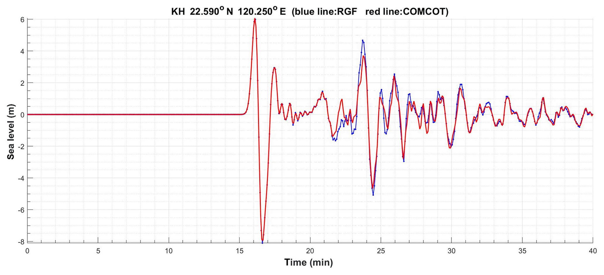
Figure 7 With the minimum water depth set to be 20 m, the RGF approach (blue) of Case 3 in KH agrees well with the direct COMCOT simulation (red).

If the shallowest water depth of the simulation domain is set to be 20 m, the coast effect is reduced and the tsunami wave will not be significantly deformed near the coast. Under this modified bathymetry, another comparison between the RGF approach and the direct COMCOT simulation is executed. As is shown in Fig. 7, the agreement between these two methods is very good after the first few waves.

It can be concluded that the forecast by the RGF approach for the first few tsunami waves is as accurate as direct simulation. After the first few waves, the interaction with the coastline may significantly affect the tsunami propagation. However, as the details of the coastline cannot be completely represented by a digitalized bathymetry with 0.06 min or coarser resolution, usually the forecast after the first few tsunami waves is irrelevant, and hence the discrepancy between the RGF and the direct COMCOT simulation can be neglected in a tsunami forecast.