the Creative Commons Attribution 4.0 License.
the Creative Commons Attribution 4.0 License.
 | 04 Mar 2020
An improved method of Newmark analysis for mapping hazards of coseismic landslides
Mingdong Zang
Shengwen Qi
Yu Zou
Zhuping Sheng
Blanca S. Zamora
Coseismic landslides can destroy buildings, dislocate roads, sever pipelines, and cause heavy casualties. It is thus important but challenging to accurately map the hazards posed by coseismic landslides. Newmark's method is widely applied to assess the permanent displacement along a potential slide surface and model the coseismic response of slopes. This paper proposes an improved Newmark analysis for mapping the hazards of coseismic landslides by considering the roughness and effect of the size of the potential slide surfaces. This method is verified by data from a case study on the 2014 Mw 6.1 (the United States Geological Survey) Ludian earthquake in Yunnan Province, China. Permanent displacements due to the earthquake ranged from 0 to 122 cm. The predicted displacements were compared with a comprehensive inventory of landslides triggered by the Ludian earthquake to map the spatial variation in the hazards of coseismic landslides using the certainty factor model. The confidence levels of coseismic landslides indicated by the certainty factors ranged from −1 to 0.95. A hazard map of the coseismic landslide was generated based on the spatial distribution of values of the certainty factor. A regression curve relating the predicted displacement and the certainty factor was drawn, and can be applied to predict the hazards of coseismic landslides for any seismic scenario of interest. The area under the curve was used to compare the improved and the conventional Newmark analyses, and revealed the improved performance of the former. This mapping procedure can be used to predict the hazards posed by coseismic landslides, and provide guidelines for decisions regarding the development of infrastructure and post-earthquake reconstruction.
- Article
(37884 KB) - Full-text XML
- BibTeX
- EndNote


Earthquakes are recognized as one of the major causes of landslides (Keefer, 1984). Hazards caused by coseismic landslides have drawn increasing attention in recent years (e.g., Jibson et al., 1998, 2000; Khazai and Sitar, 2003; Qi et al., 2010, 2011, 2012; Chen et al., 2012; Xu et al., 2013; Yuan et al., 2014). The damage caused by seismically triggered landslides is sometimes more severe than the direct damage caused by the earthquake (Keefer, 1984). Estimating where a specific shaking is likely to induce a slope failure plays an important role in the regional assessment of coseismic landslides.
Pseudo-static analysis formalized by Terzaghi (1950), and finite-element modeling applied by Clough and Chopra (1966) have been employed to assess the seismic stability of slopes in early efforts (Jibson, 2011). Newmark (1965) first introduced a relatively simple and practical method, which is still commonly used nowadays to estimate the coseismic permanent displacements of slopes (Jibson, 2011). Studies have shown that Newmark's method yields reasonable and practical results when modeling the dynamic performance of natural slopes (Wilson and Keefer, 1983; Wieczorek et al., 1985; Jibson et al., 1998, 2000; Pradel et al., 2005). Rathje and Antonakos (2011) recently presented a unified framework for predicting coseismic permanent sliding displacement based on Newmark's method. Chen et al. (2018) used Newmark's method to calculate the minimum accelerations required for coseismic landslides in the region affected by the 2014 Ludian earthquake. Chen et al. (2019) subsequently developed an easy operation mapping method to assess hazards posed by coseismic landslides in the zone struck by the 2014 Ludian earthquake using Newmark's method.
Such applications generally start from an analysis of the dynamic stability of slopes, which is quantified as the critical acceleration. Barton model (Barton, 1973) has been widely used in rock mechanics and engineering to predict the shear strength of rock joints, which plays a crucial role in the calculation of critical acceleration. However, researchers have not adequately attended to the shear strength of rock joints during the assessment of coseismic landslides. To better estimate the dynamic stability of slopes, in this paper, we introduce the Barton model (Barton, 1973) to Newmark analysis to develop an improved modeling method for mapping the hazards posed by coseismic landslides using data from the 2014 Ludian earthquake in Yunnan Province in southwestern China. As predictions of coseismic landslides are not based on exact results, i.e., the computed permanent displacements, but are also mingled with unformalized expertise, i.e., the interpreted landslides, we present a model of inexact reasoning, i.e., the certainty factor model (CFM), that defies analysis, as an application of sets of inference rules that are expressed in predicate logic (Shortliffe and Buchanan, 1975) to produce a map of the hazards posed by coseismic landslides.
This paper briefly introduces the characteristics and spatial distribution of landslides triggered at the chosen site, describes the method of modeling used for the analysis of the stability of seismic slopes, presents the mapping procedure of the confidence level of seismic slope failure, and finally discusses the results of the assessment of seismic hazard, as well as a comparison with the conventional Newmark analysis.
The epicenter of the 2014 Mw 6.1 (the United States Geological Survey) Ludian earthquake was located on the southeastern margin of the Tibetan Plateau. A rectangular area lying immediately around the epicenter containing dense concentrations of the induced landslides was chosen for study (Fig. 1). The elevation of the area ranged from 785 to 3085 m above sea level. Three rivers – the Niulanjiang River, Shaba River, and Longquan River – pass through the study area (Fig. 1). The topography ranges from flat in the river valleys to nearly vertical in the slopes on the banks of the rivers. According to Chen et al. (2015), Niulanjiang River flows from the southeast (SE) to the northwest (NW), and incises to a depth between 1200 and 3300 m, resulting in about 80 % of the slopes having angles greater than 40∘ distributed along the banks. The predominant geological units of the study area have an age that varies from the Proterozoic to the Mesozoic, including dolomite, limestone, shale, sandstone, basalt, and slate (Fig. 2).
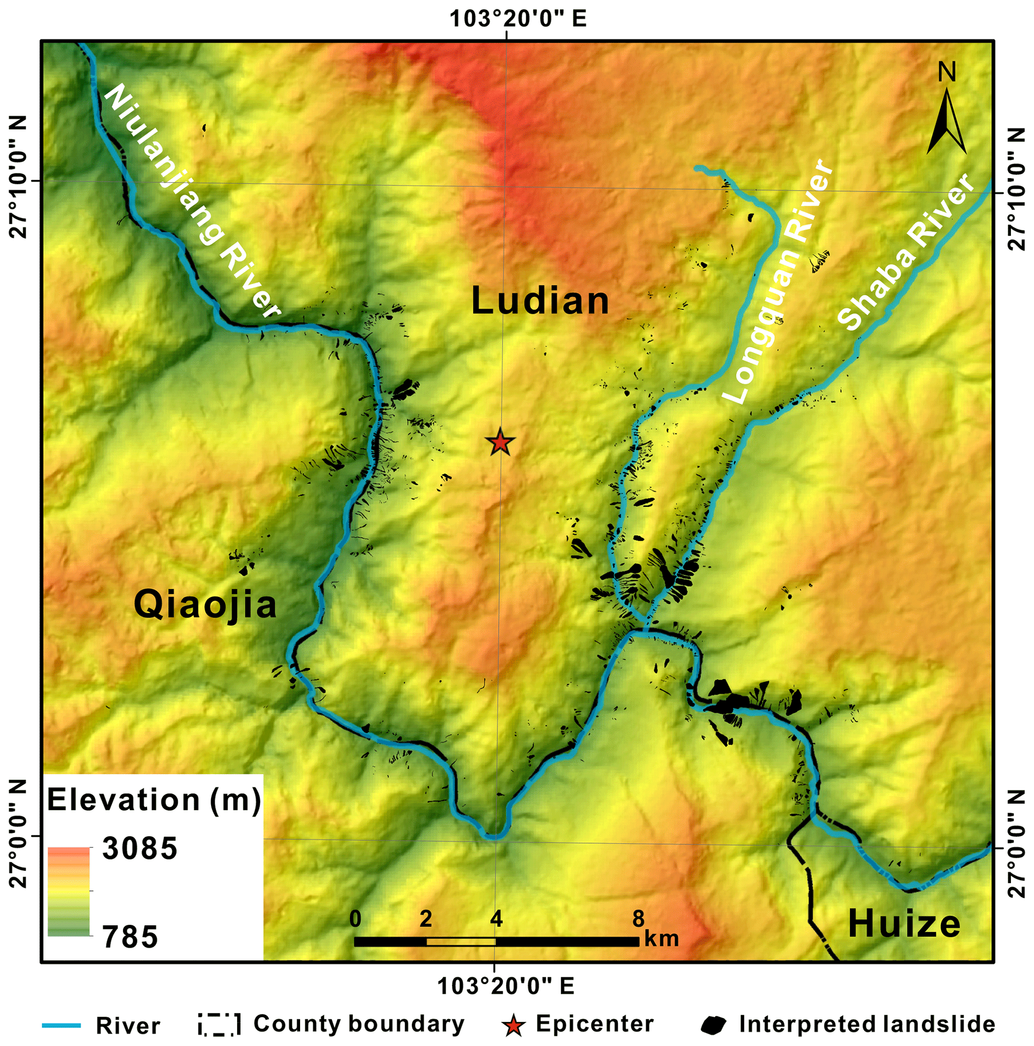
Figure 1Map of the study area showing the inventoried landslides.
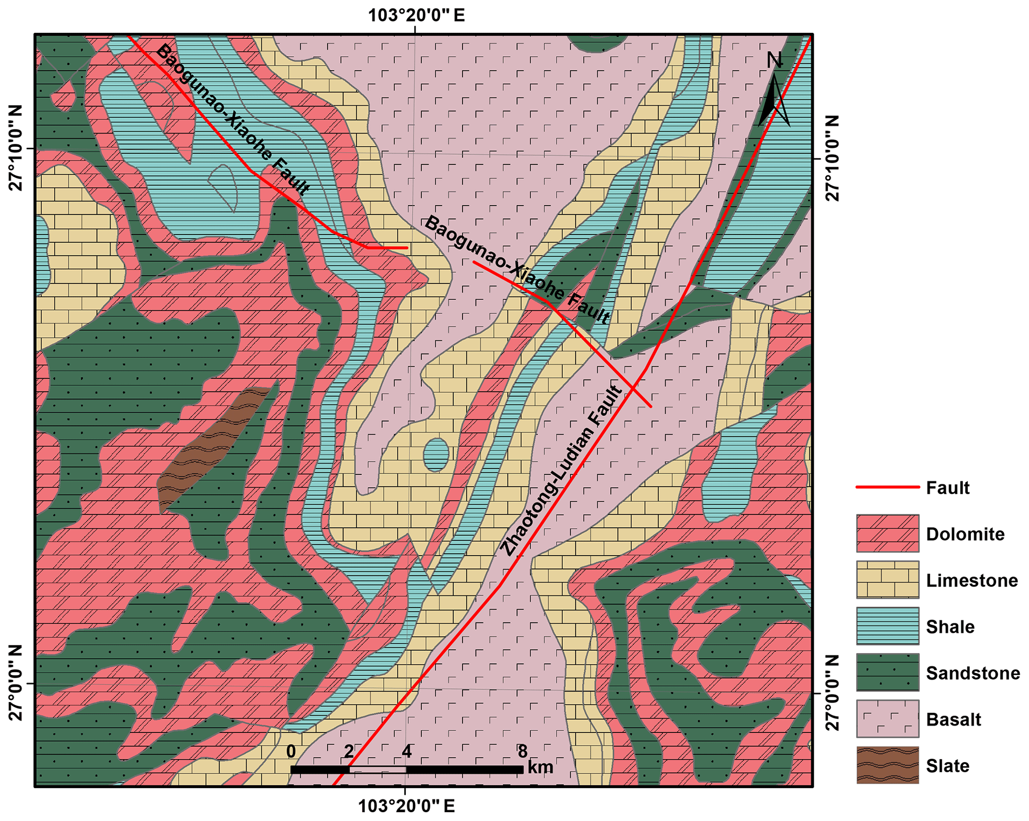
Figure 2Geological map of the study area showing lithology and faults.
An inventory of 1416 landslides triggered by the 2014 Ludian earthquake (Fig. 1) was compiled by visual inspection through comparisons between pre-earthquake satellite images obtained from Google Earth (30 January 2014) and 0.2 m high-resolution post-earthquake aerial images (7 August 2014; data provided by the Digital Mountain and Remote Sensing Applications Center, Institute of Mountain Hazards and Environment, Chinese Academy of Sciences, and Beijing Anxiang Power Technology Co., ltd.). A majority of landslides triggered by the earthquake were shallow, flow-like landslides (shallower than 3 m), developing in particularly dense concentrations along steeply incised river valleys. The total area of these interpreted landslides was 7.01 km2 within a study area of 705 km2. A detailed study showed that 846 of the mapped landslides were greater than 1000 m2 in area, occupying 6.74 km2 and accounting for 96.1 % of the total area of landslides, of which 279 were greater in area than 5000 m2, occupying 5.37 km2 and accounting for 76.6 % of the total landslide area.
3.1 Modeling method
In the context of the analysis of the dynamic stability of a slope, Newmark (1965) proposed a permanent displacement analysis that bridges the gap between simplistic pseudo-static analysis and sophisticated but generally impractical finite-element modeling (Jibson, 1993). Newmark's method simulates a landslide as a rigid plastic friction block with a known critical acceleration on an inclined plane (Fig. 3) and calculates the cumulative permanent displacement of the block, as it is subjected to an acceleration time history of an earthquake. Newmark (1965) showed that the dynamic stability of a slope is related to the critical acceleration of a potential landslide block and can be expressed as a simple function of the static factor of safety and the geometry of the landslide (Jibson et al., 1998, 2000):
where ac is the critical acceleration in terms of g, i.e., the acceleration due to the Earth's gravity, FS is the static factor of safety, and α is the angle from the horizontal at which the center of the slide block moves when displacement first occurs (Jibson et al., 1998, 2000). For a planar slip surface parallel to the slope, this angle generally approximates to the angle of the slope.
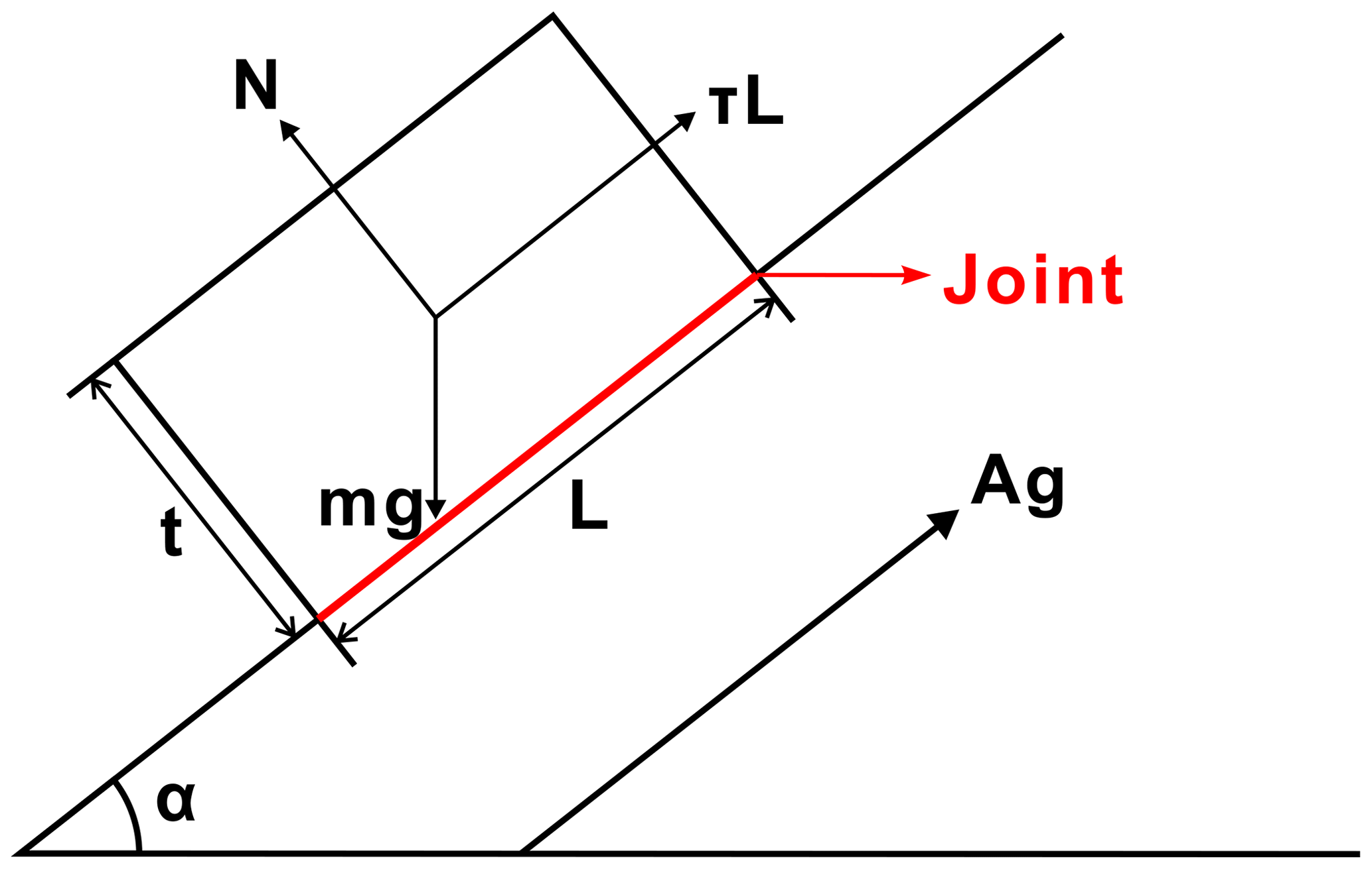
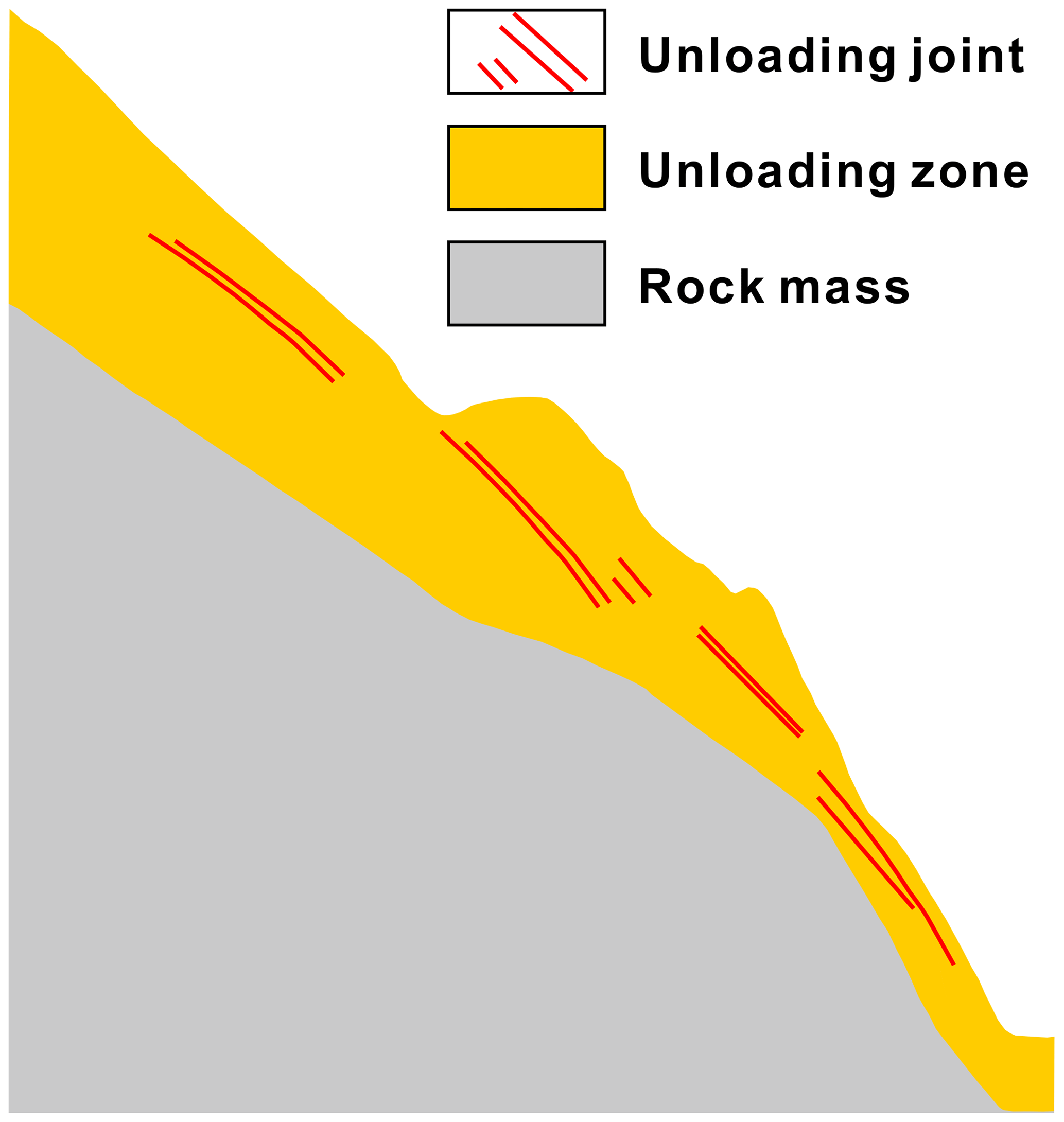
Natural slopes often develop a group of shallow unloading joints (Fig. 4) parallel to the surface due to valley incisions (Gu, 1979; Hoek and Bray, 1981). Studies have shown that rock slopes behave as collapsing and sliding failures of shallow unloading joints under strong earthquakes, and 90 % of coseismic landslides are shallow falls and slides (Harp and Jibson, 1996; Khazai and Sitar, 2003; Dai et al., 2011; Tang et al., 2015). According to Qi et al. (2012), two typical kinds of landslides are triggered by earthquakes: (a) shallow, flow-like landslides with a depth of less than 3 m in general and (b) rockfalls thrown by the shaking caused by the earthquake that usually occur at the crest of the slope. For both types, unstable blocks of rock are often cut and activated along the rock joints. Therefore, the static factor of safety in terms of the critical acceleration in these conditions is related to the peak shear strength of the rock joints. For the purpose of regional analysis, we use a limit equilibrium model of an infinite slope (Fig. 3) by referring to the simplification of Newmark's method by of Jibson et al. (1998, 2000). The value of the static factor of safety against sliding given by the ratio of resistance to the driving forces is determined by conventional analysis without considering accelerations, expressed as follows:
where τ is the peak shear strength of the rock joint, L is the length of the rock joint, m is the mass of the failure rock block, γ is the unit weight of the rock mass, and t is the thickness of the failure rock block.
For a Newmark analysis, it is customary to describe the shear strength of rocks instead of rock joints in terms of Coulomb's constants, i.e., friction angle (φ) and cohesion (c). However, both are not only stress dependent but also scale dependent (Barton and Choubey, 1977). According to Barton (1973), a more satisfactory empirical relationship for predicting the peak shear strength of a joint can be written as follows:
where σn is the effective normal stress, JRC is the joint roughness coefficient, JCS is the joint wall compressive strength, and ϕb is the basic friction angle, i.e., the angle of frictional sliding resistance between rock joints, which can be obtained from residual shear tests on natural joints (Barton, 1973).
The effective normal stress (σn) generated by gravity acting on the rock block is as follows:
Considering the impact of size on JRC and JCS, the formulations developed by Barton and Bandis (1982) are shown as follows:
where the nomenclature adopted incorporates (0) and (n) for values of the laboratory scale and the in situ scale, respectively.
Hence, the static factor of safety (FS) of a slope can be written as follows:
After calculating the angle of the slope and static factor of safety, the critical acceleration of the slope can be determined. Once the time history of the earthquake' acceleration has been selected, portions of the record lying above the critical acceleration ac (Fig. 5a) are integrated once to derive a velocity profile (Fig. 5b); the time history of velocity is then integrated a second time to obtain the profile of cumulative displacement of the block (Fig. 5c). Users finally determine the dynamic performance of the slope based on the magnitude of the Newmark displacement (Jibson et al., 1998, 2000; Jibson, 2011). The detailed procedure for conducting a Newmark analysis with the Barton model is discussed in the following sections.
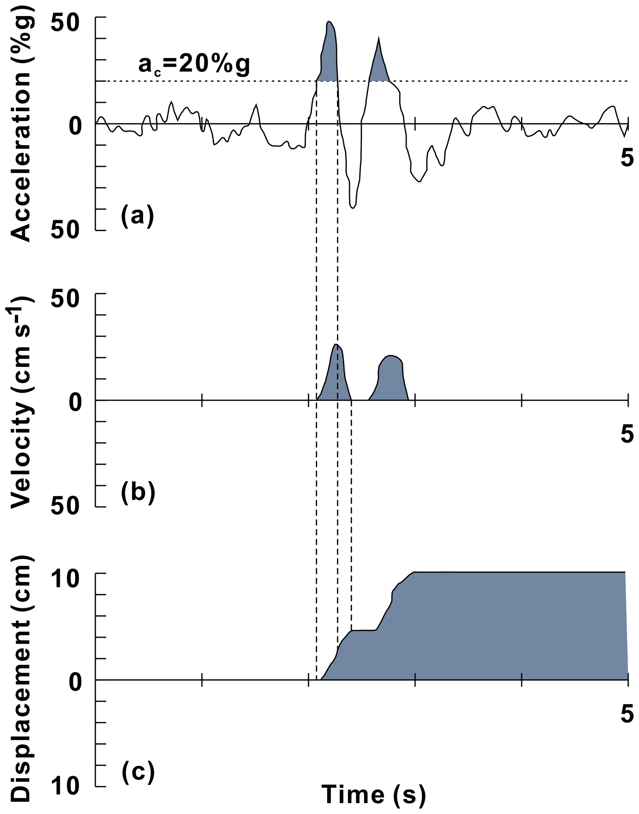
Figure 5Demonstration of the Newmark analysis algorithm (adapted from Wilson and Keefer, 1983; Jibson et al., 1998, 2000).
3.2 Static factor-of-safety map
Considering that the mapped landslides greater than 1000 m2 in area occupied 96.1 % of the total landslide area, we selected a 30 m × 30 m digital elevation model (DEM) from the ASTER Global Digital Elevation Model (https://doi.org/10.5067/ASTER/ASTGTM.002; NASA/METI/AIST/Japan Spacesystems and U.S./Japan ASTER Science Team, 2009), which facilitated the subsequent hazard analysis. A basic slope algorithm was applied to the DEM to produce a slope map (Fig. 6), where the slope was identified as the steepest downhill descent from a cell to its neighbors (Burrough and McDonell, 1998). The slopes ranged from greater than 60∘ along the banks of the Niulanjiang River, Shaba River, and Longquan River to less than 20∘ in low mountains and hills in the north and east.
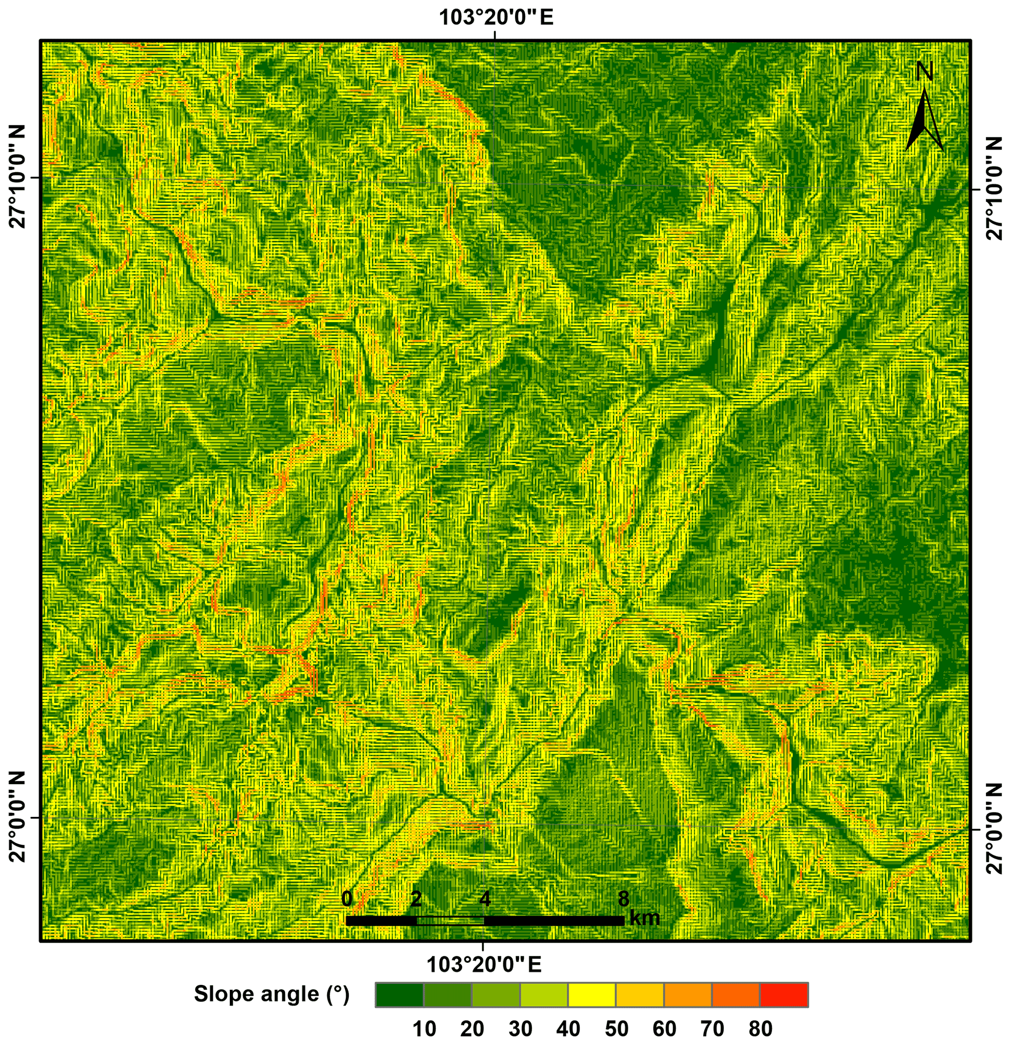
Figure 6Slope map derived from the DEM of the study area.
According to Jibson et al. (1998, 2000), slopes steeper than 60∘ remain unstable even at high strengths. We assume that Newmark's rigid plastic block is unsuitable for such a steep sliding surface. In this case, sliding occurs along a plane at an angle (α) of with the horizon (Fig. 7). Therefore, we assigned an angle (α) of to slopes steeper than 60∘ to avoid too small a value of FS in the Newmark analysis.
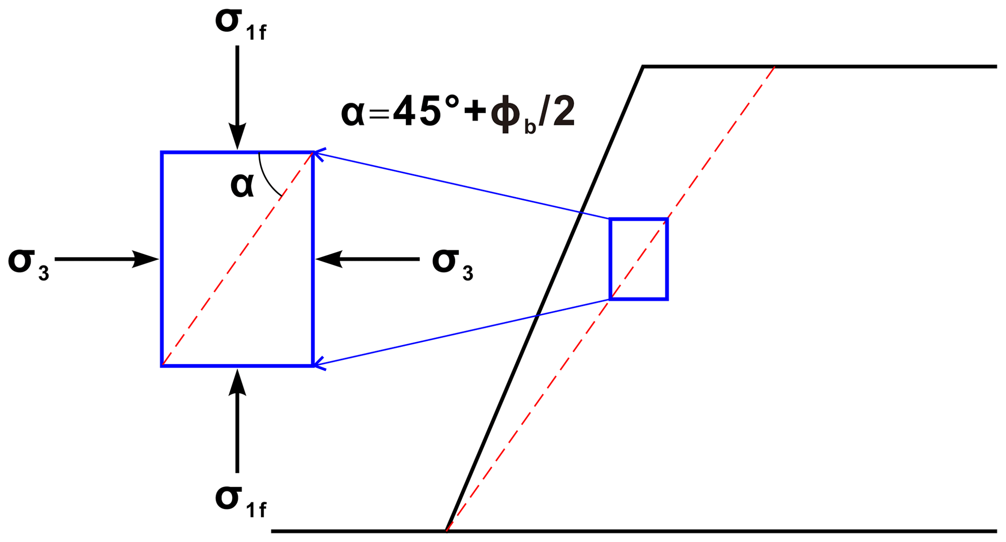
Figure 7Schematic map showing the angle (α) for slopes steeper than 60∘. σ1f and σ3 are the major and minor principal stress in the state of limit equilibrium, respectively. ϕb is the basic friction angle.
Table 1Shear strengths assigned to rock types in the study area.
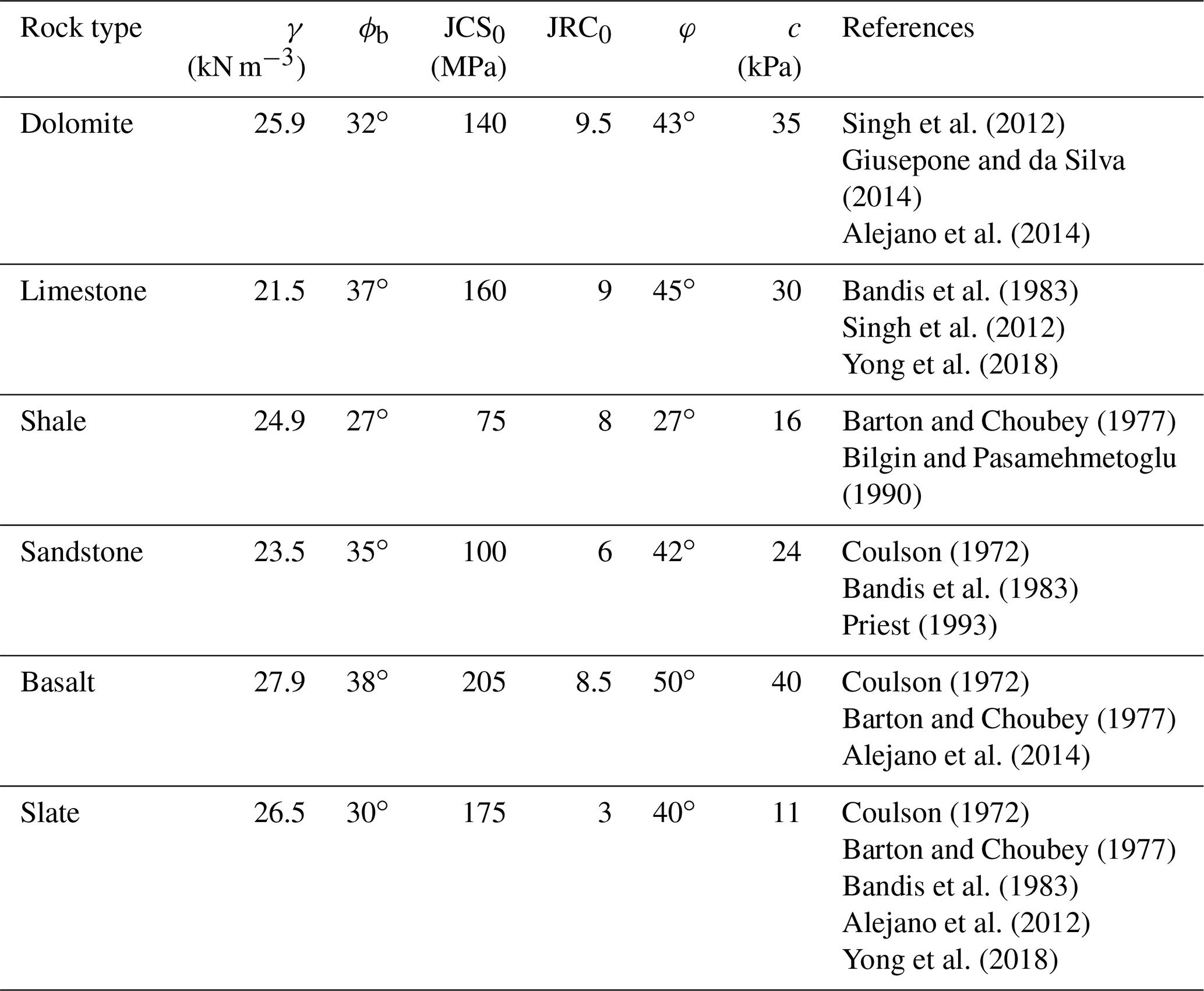
Friction angle (φ), cohesion (c), and unit weight (γ) were derived from the Geological Engineering Handbook (Geological Engineering Handbook Editorial Committee, 2018).
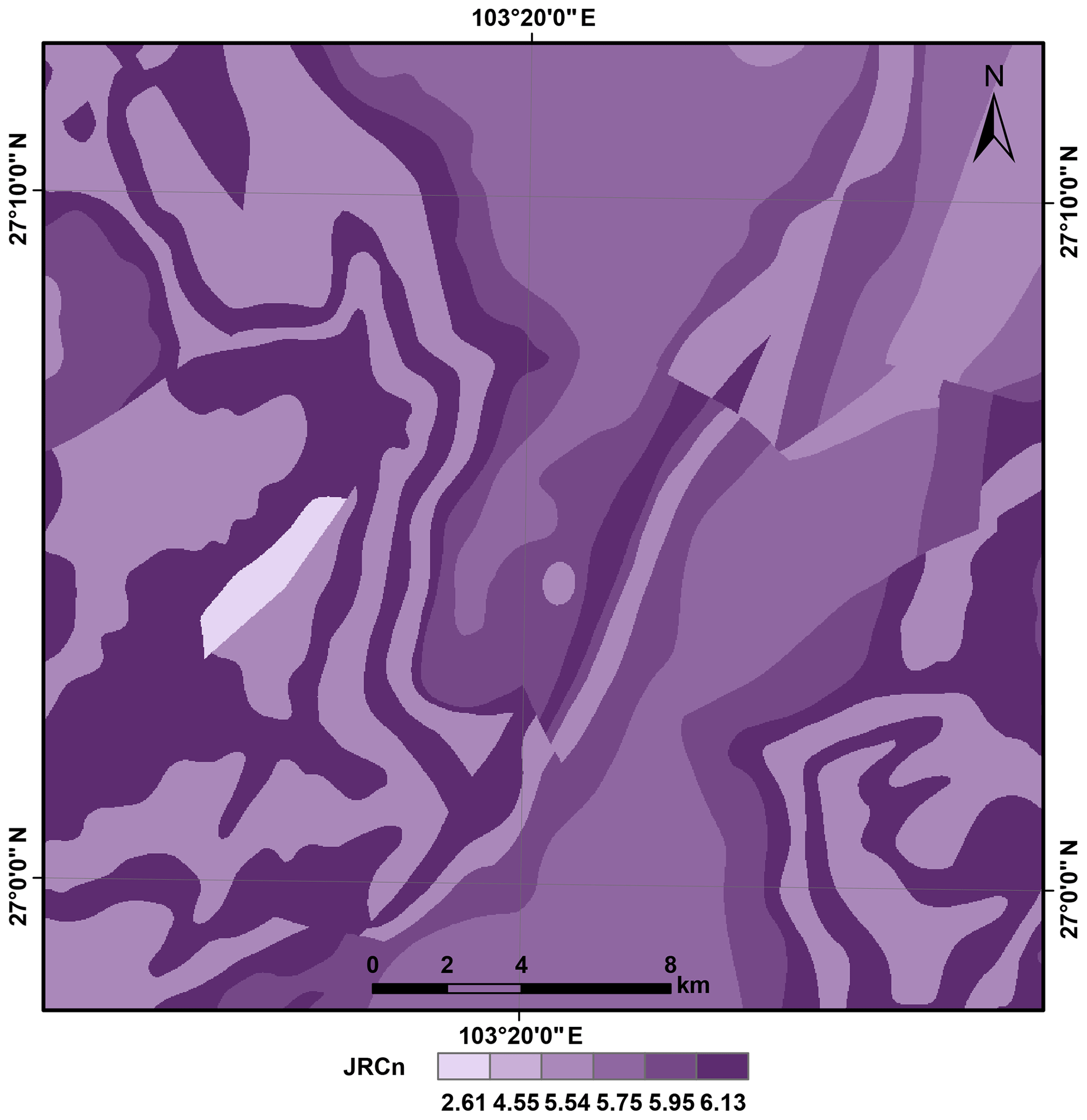
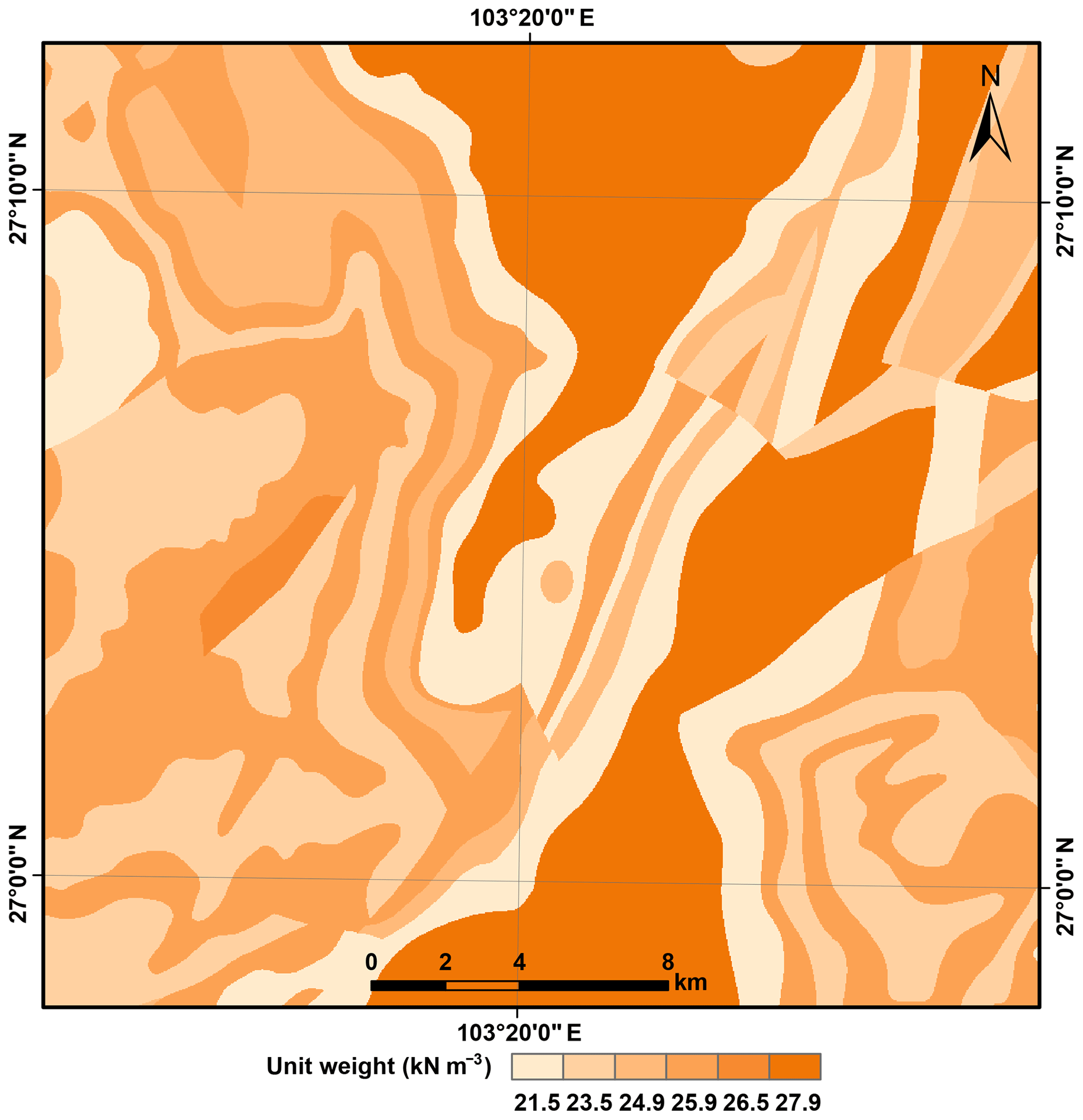
The digital geological map from the China Geological Survey (CGS) was rasterized at a 30 m grid spacing to assign material properties throughout the study area. According to the literature, JRC0 and JCS0 depend strongly on lithology (Coulson, 1972; Barton and Choubey, 1977; Bandis et al., 1983; Bilgin and Pasamehmetoglu, 1990; Priest, 1993; Singh et al., 2012; Alejano et al., 2012, 2014; Giusepone and da Silva, 2014; Yong et al., 2018). Representative values of γ, JRC0, JCS0, and ϕb assigned to each rock type exposed in the study area were estimated using the test data listed in Table 1. The selected values were near the middle of the ranges represented in the references. These JRC0 and JCS0 values were considered in a laboratory scale for a length of 100 mm as L0. For each grid cell in the regional analysis, the length of the engineering dimension, Ln, can generally be set as a 10-fold range of L0. This is because the value of JRCn∕JRC0 (JCSn∕JCS0) is nearly constant when the value of Ln∕L0 is greater than 10 (Bandis et al., 1981). The values of JRCn and JCSn were then calculated by inserting the values of JRC0 and JCS0, and L0, and Ln into Eqs. (5) and (6), respectively. Figures 8 and 9 show the spatial distributions of JRCn and JCSn, respectively. The basic friction angle (ϕb) map and unit weight (γ) map are shown in Figs. 10 and 11, respectively.
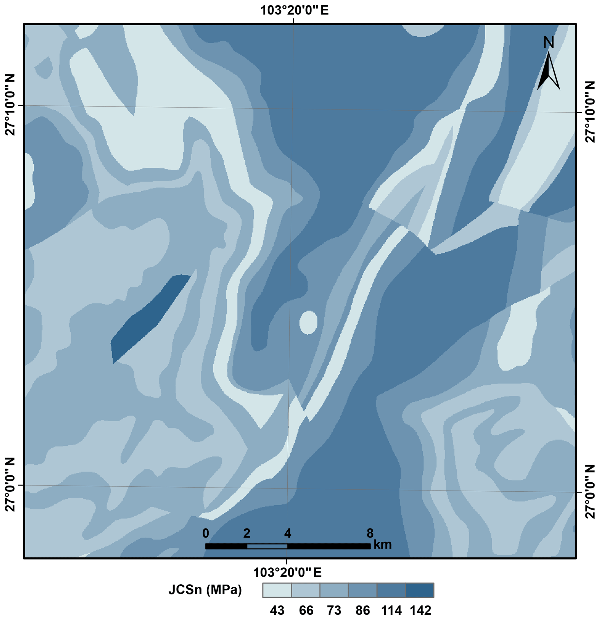
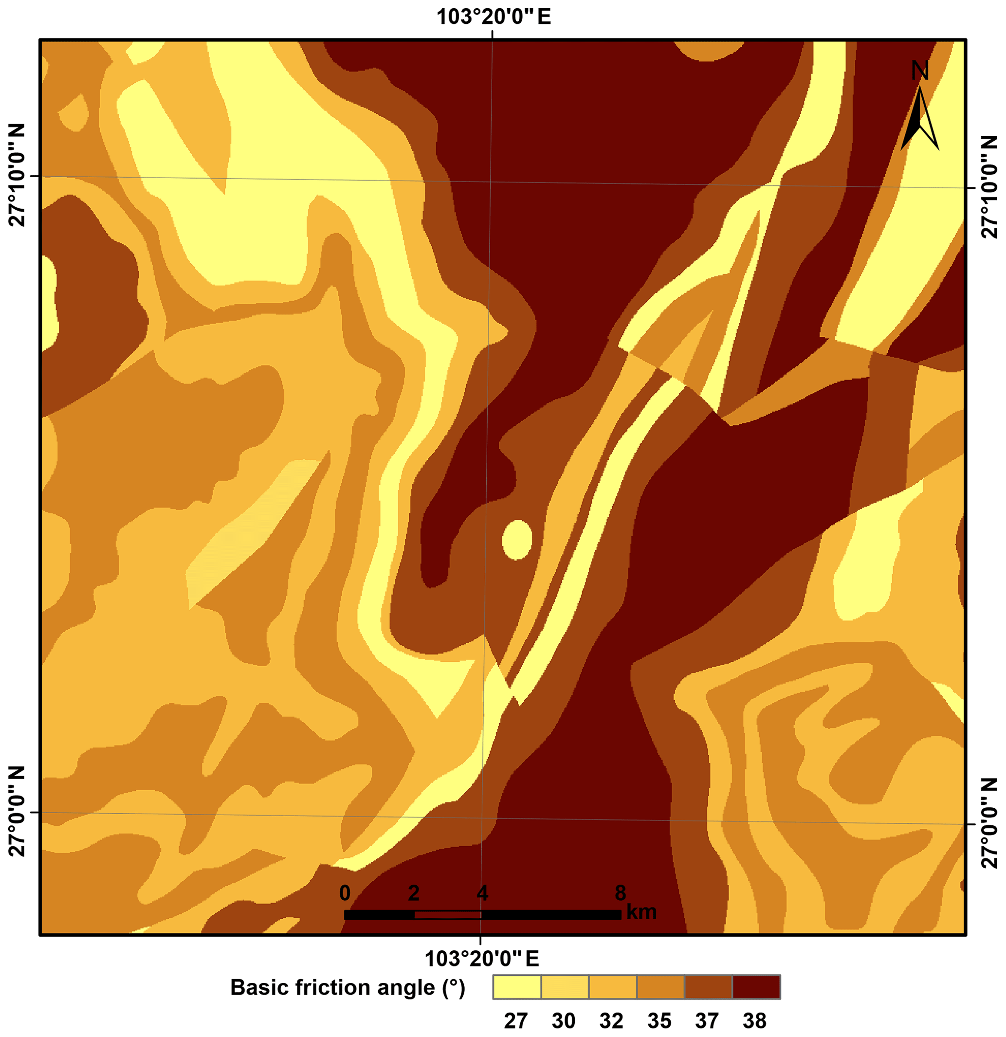
Figure 10Basic friction angle (ϕb) component of shear strength assigned to rock types in the study area.
For the sake of simplicity, the thickness of the modeled block t was taken to be 3 m, which reflected the typical slope failures of the Ludian earthquake. The static factor-of-safety map was produced by combining these data layers (α, JRCn, JCSn, ϕb, and γ) in Eq. (7). In the initial iteration of the calculation, grid cells in steep areas with static factors of safety smaller than 1 indicated that the slopes were statically unstable, but this did not necessarily mean that they were moving under shaking induced by the earthquake. In this condition, to avoid conservative results, we neither increased the strengths of the rock types with statically unstable cells nor adjusted the strengths of other rock types to preserve the differences in relative strength between them (as in Jibson et al., 1998, 2000). Instead, we assigned a minimal static factor of safety of 1.01, merely above limit equilibrium (Jibson et al., 1998, 2000), to these slopes to avoid a negative value of the critical acceleration ac. According to Keefer (1984), most landslides triggered by earthquakes occur with a slope of at least 5∘. The static factors of safety resulting from slopes of angles smaller than 5∘ were very high. These slopes were unlikely to fail under the Ludian earthquake and did not produce a statistically significant sample in the analysis. Therefore, slopes less steep than 5∘ were not analyzed in the second iteration. After the adjustment, the static factors of safety ranged from 1 to 17.4, as shown in Fig. 12.

Figure 12Static factor-of-safety map of the study area.
3.3 Critical acceleration map
According to Newmark (1965), a pseudo-static analysis in terms of the static factor of safety and the slope angle was employed to calculate the critical acceleration of a potential landslide. The map of critical acceleration (Fig. 13) was generated by combining the static factor of safety and the slope angle in Eq. (1). The critical accelerations were derived from the intrinsic properties of the slope (topography and lithology), regardless of the given shaking. Therefore, the map of critical acceleration indicated the susceptibility of coseismic landslides (Jibson et al., 1998, 2000). The calculated critical accelerations ranged from nearly zero in areas that were more susceptible to coseismic landslides to greater than 1 g in areas that were less susceptible.
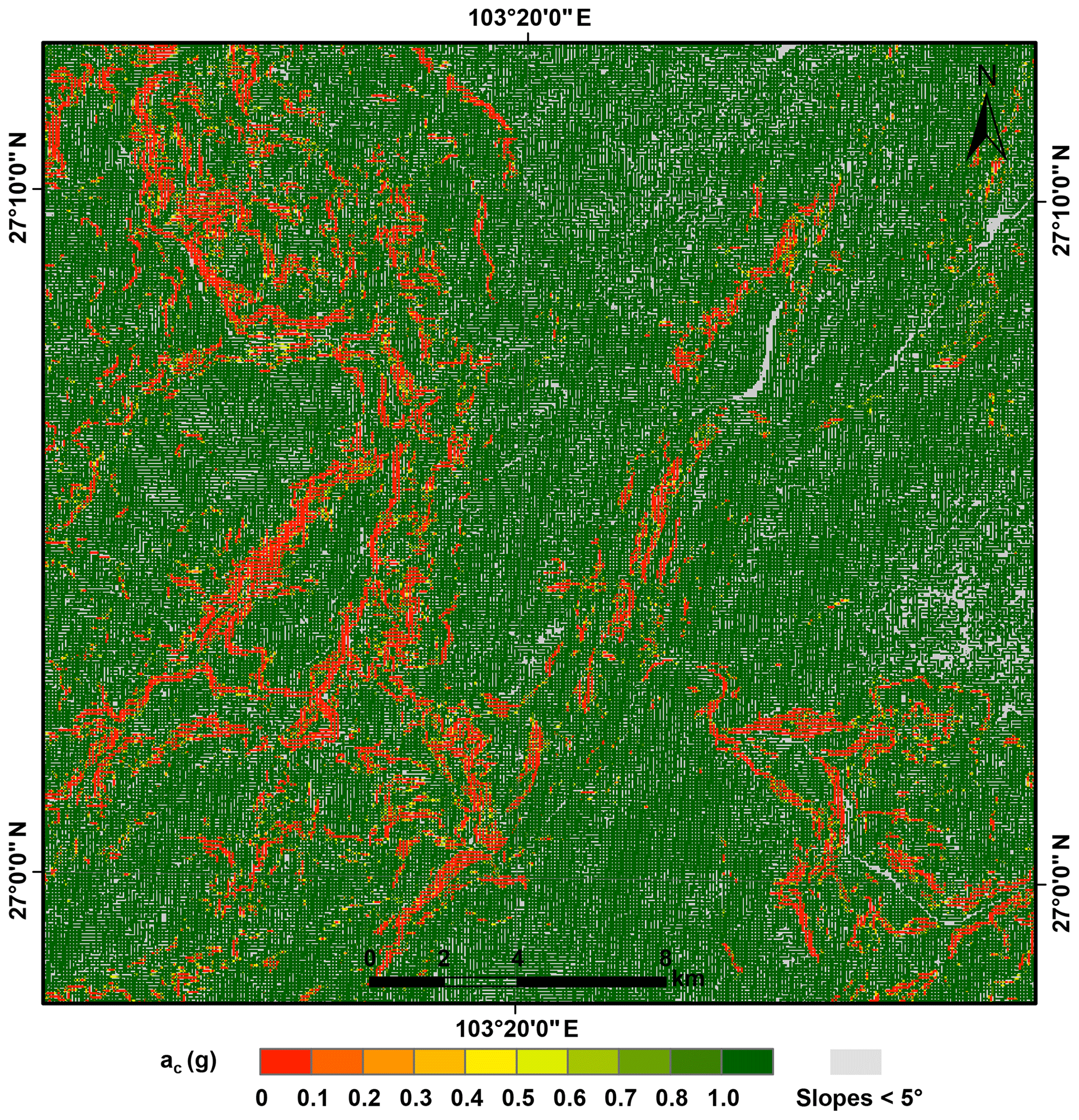
Figure 13Map showing critical accelerations in the study area.
3.4 Shake map
There were 23 strong motion stations within 100 km of the epicenter of the Ludian earthquake (Fig. 14). Each station's record contained the three components of the peak ground acceleration (PGA), south–north direction, east–west direction, and up–down direction, as listed in Table 2 (the dataset was provided by the China Earthquake Data Center, http://data.earthquake.cn, last access: 16 June 2016). We calculated the average PGA of the two horizontal components of each strong motion recording and plotted a contour map (Fig. 15) using an inverse distance-weighted (IDW) interpolation algorithm. It determined the cell values using a linearly weighted combination of a set of sample stations with weights inversely proportional to distance (Watson and Philip, 1985). In addition, given that input stations far from the epicenter, where the prediction was made, might have had poor or no spatial correlation, we eliminated the input stations beyond 100 km from the epicenter from the calculation.
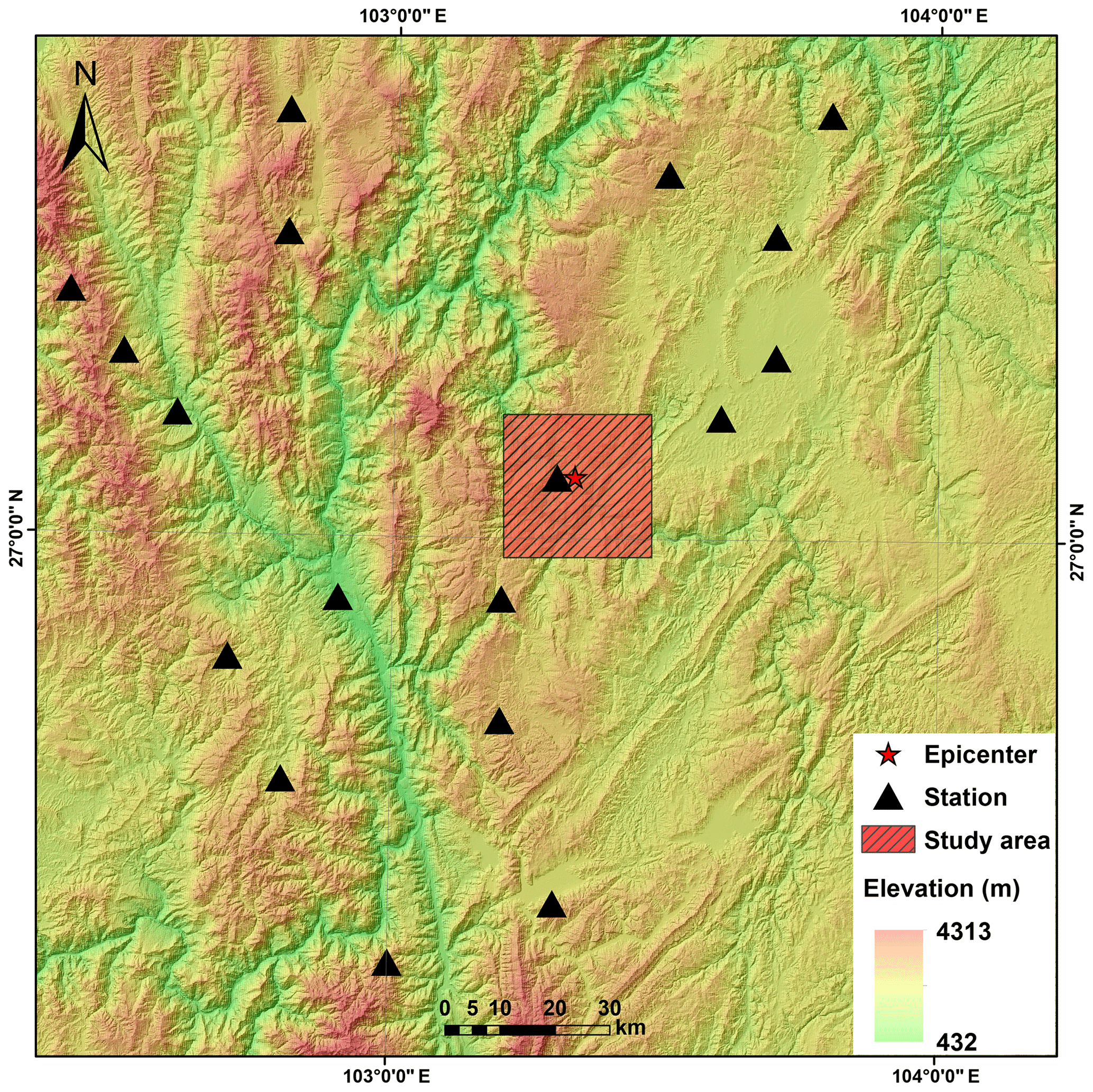
Figure 14Locations of strong motion stations.
Table 2Station records of three components of peak ground acceleration.
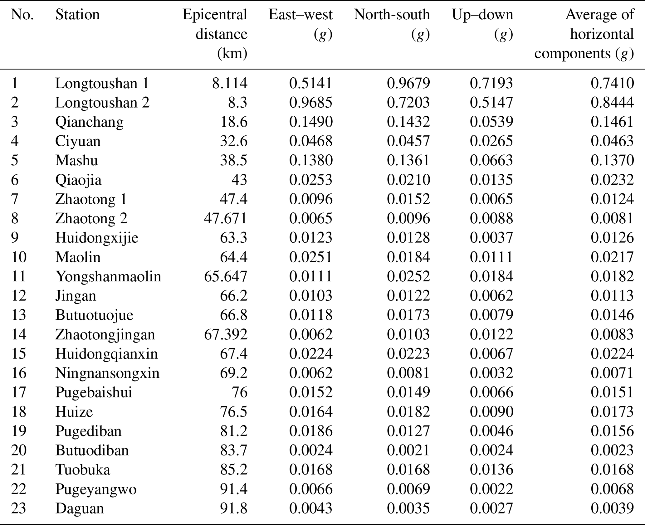
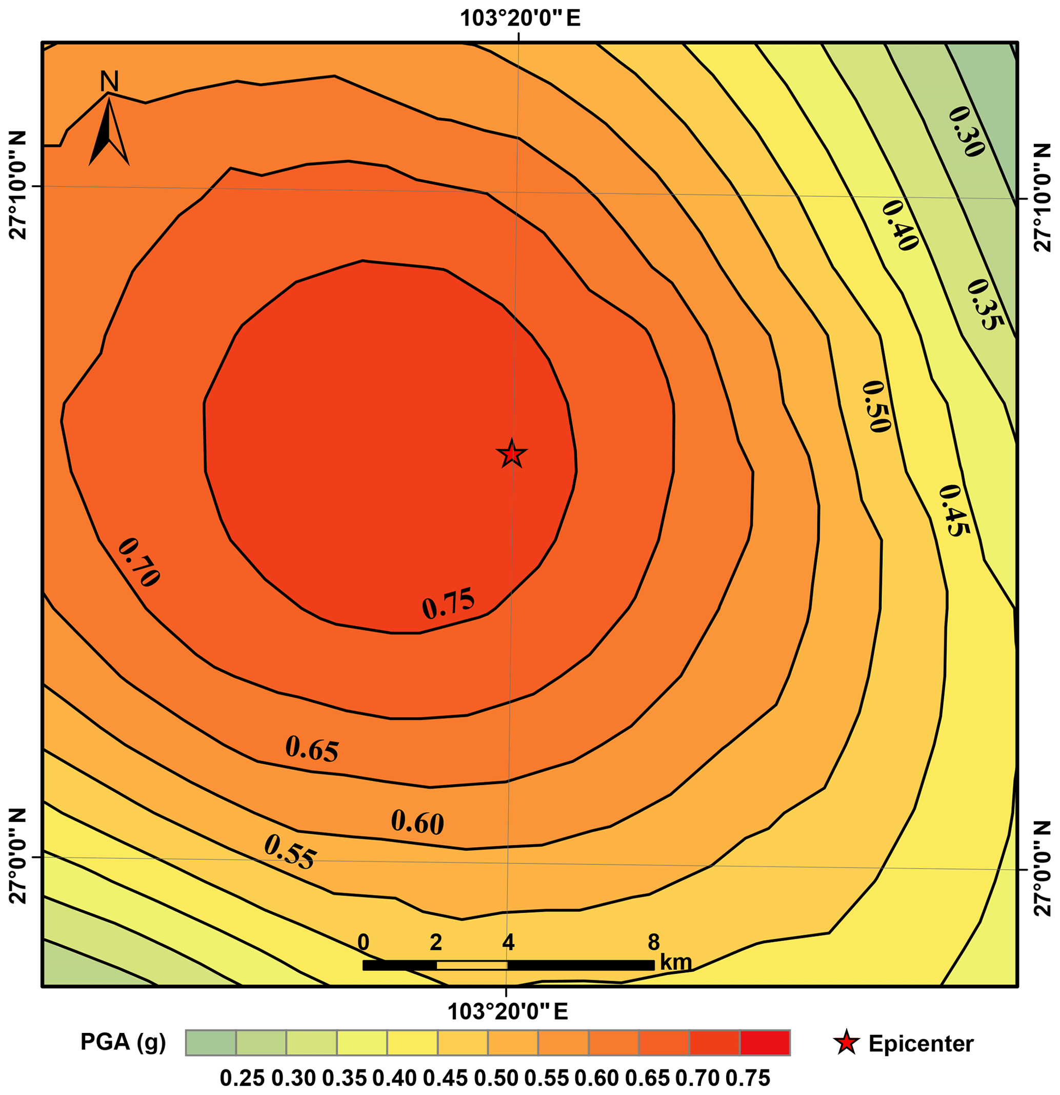
Figure 15Contour map of peak ground acceleration (PGA) produced by the Ludian earthquake in the study area. PGA values shown are in g.
3.5 Newmark displacement map
In case of a landslide, in practice it is impossible to conduct a rigorous Newmark analysis when accelerometer records are unavailable. It is also impractical and time consuming to produce a displacement in each cell during the regional analysis. Therefore, empirical regressions (Ambraseys and Menu, 1988; Bray and Travasarou, 2007; Jibson, 2007; Saygili and Rathje, 2008; Rathje and Saygili, 2009; Hsieh and Lee, 2011) have been proposed to estimate Newmark displacement as a function of the critical acceleration and peak ground acceleration or the Arias intensity. Rathje and Saygili (2009) developed a vector model for displacement in terms of the critical acceleration (ac), peak ground acceleration (PGA), and moment magnitude (Mw) based on an analysis of over 2000 strong motion recordings:
where D is the predicted displacement in centimeters, and ac and PGA are in units of g.
This model is a preferred displacement model at a site where acceleration time recordings are not available. Incorporating multiple parameters of ground motion into the analysis typically results in less variation in the prediction of displacement (Rathje and Saygili, 2009).
The Newmark displacement of each cell was calculated by combining the corresponding values of the critical acceleration, peak ground acceleration, and moment magnitude in Eq. (8). The predicted displacements ranged from 0 to 122 cm, as shown in Fig. 16.
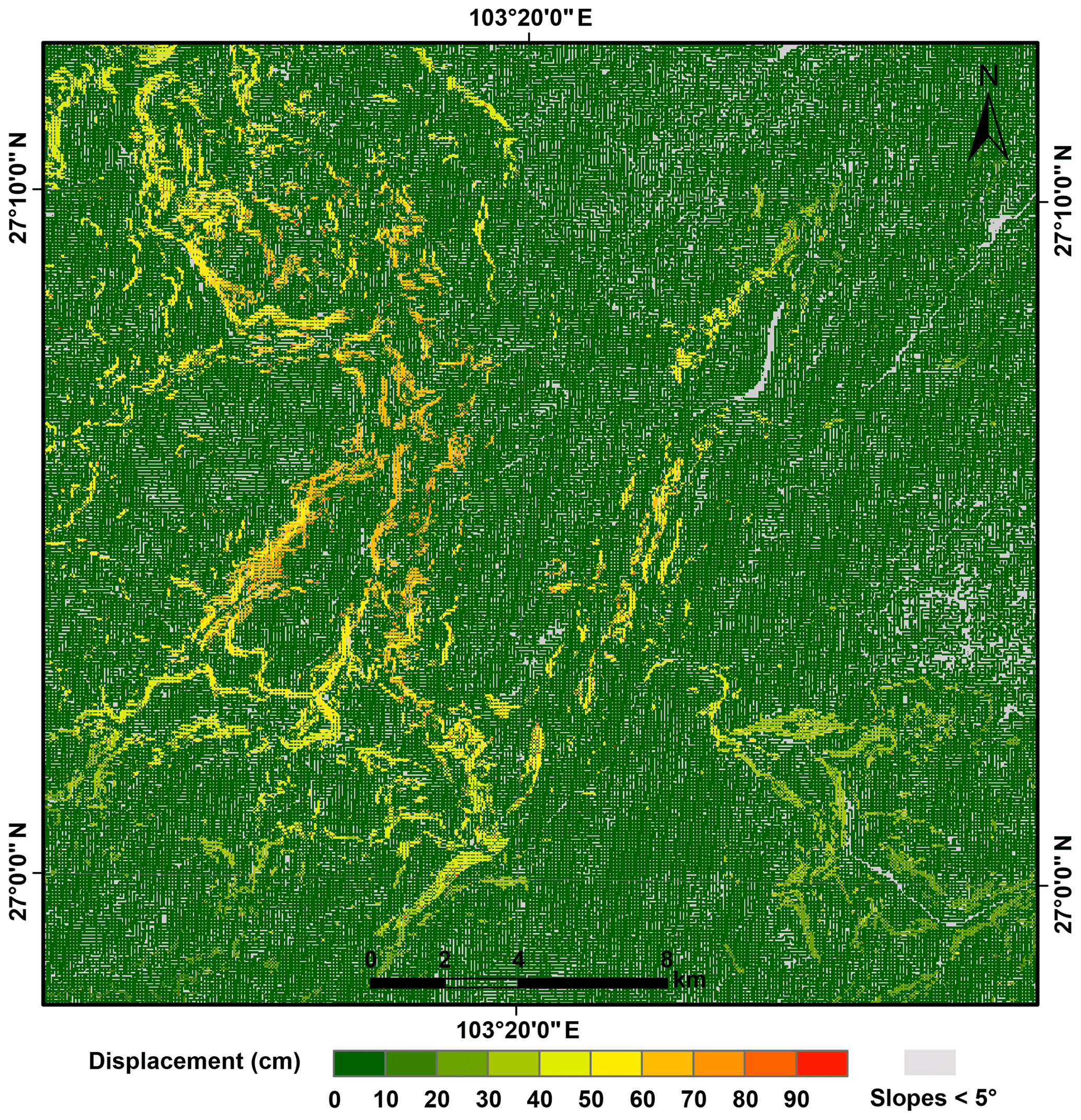
Figure 16Map showing predicted displacements in the study area.
3.6 Coseismic landslide hazard map
According to Jibson et al. (1998, 2000), predicted displacements provide an index of the seismic performance of slopes, where larger predicted displacements relate to a greater incidence of slope failures. But the displacements do not correspond directly to measurable slope movements in the field. To produce a coseismic landslide hazard map, we chose a model of inexact reasoning, the certainty factor model (CFM) created by Shortliffe and Buchanan (1975) and improved by Heckerman (1986), to explore the relationship between the occurrences of landslides and their predicted displacements. The CFM was created as a numerical method, initially used in MAYCIN, a backward-chaining expert system used in medical contexts (Shortliffe and Buchanan, 1975), for managing uncertainty in a rule-based system. In this model, the certainty factor (CF) represents the net confidence in a hypothesis H based on the evidence E (Heckerman, 1986). Certainty factors range between −1 and 1. A CF with a value of −1 means a total lack of confidence, whereas a CF with a value of 1 means total confidence. Values greater than zero favor the hypothesis while those less than zero favor its negation. According to Heckerman (1986), the probabilistic interpretation of CF is as follows:
where CF is the certainty factor, p(H|E) denotes the conditional probability for a posterior hypothesis that relies on evidence, the posterior probability, and p(H) is the prior probability before any evidence is known. In the displacement analysis, p(H|E) was defined as the proportion of the area of the landslide within a specific displacement area and p(H) was defined as the proportion of the landslide area within the entire study area, excluding slopes less steep than 5∘. In this way, the values of CF represented the confidence level for coseismic landslides. Positive values corresponded to an increase in the confidence level in slope failure while negative quantities corresponded to a decrease in this confidence. Higher positive values indicated higher confidence levels for coseismic landslides.
Given the above definition, we produced a coseismic landslide hazard map in terms of the certainty factors. First, displacement cells every 1 cm were grouped into bins such that all cells with displacements between 0 and 1 cm were grouped into the first bin, those with displacements between 1 and 2 cm were grouped into the second bin, and so on. The displacements were grouped into 123 bins, from 0 to 122 cm. We then calculated the proportion of cells occupied by areas of landslides in each bin. This proportion was considered the posterior probability of each bin as previously defined. The prior probability calculated by dividing the entire landslide area by the entire study area was the same in each bin. Finally, the values of CF were computed in each bin by using Eq. (9) to combine the corresponding values of the posterior and prior probabilities. The certainty factors ranged from −1 to 0.95. The values of CF indicated the confidence level of the occurrence of a landslide for each bin in the study area and provided the basis for producing the coseismic landslide hazard map.
As shown in the hazard map (Fig. 17), 73.2 % of landslides triggered by the Ludian earthquake were in areas with higher confidence levels with CF values greater than 0.6. The interpreted landslides were covered on the map to demonstrate their goodness of fit for the predicted confidence levels for coseismic landslides (Fig. 17).
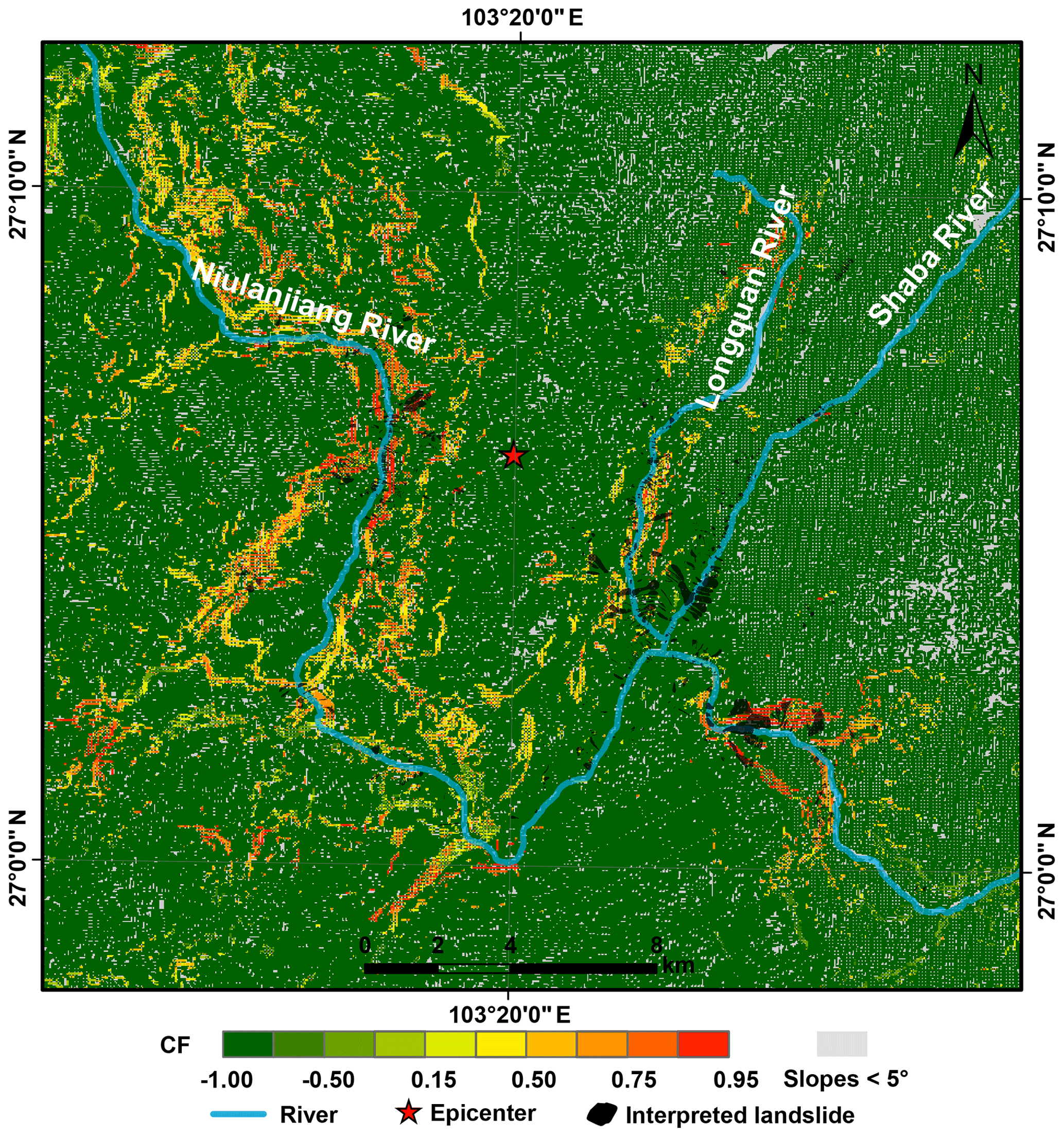
Figure 17Map showing confidence levels of coseismic landslides during the Ludian earthquake using the proposed method. Confidence levels are portrayed in terms of values of CF.
The predicted displacements represent the cumulative sliding displacements for a given time history of acceleration. Based on the statistically significant sizes of the areas, displacements less than 60 cm, which was around the middle of the range of displacement, occupied about 80 % of the study area, while displacements greater than 80 cm occupied a very small area. Jibson et al. (1998, 2000) assumed that shallow falls and slides in brittle, weakly cemented materials fail following a relatively small displacement, whereas slumps and block slides in more compliant materials likely fail following a larger displacement. That is to say, the study area was more susceptible to rockfalls and shallow, disrupted slides that fail following a relatively small displacement. By contrast, it was subjected at a lower probability to coherent, deep-seated slides that would fail following a larger displacement. Indeed, the majority of landslides triggered by the Ludian earthquake were shallow, disrupted slides and rockfalls (Zhou et al., 2016). Although a few catastrophic rock avalanches, such as the Hongshiyan landslide (Chang et al., 2017), occurred in the field, they did not produce statistically significant samples that could meaningfully contribute to the model, which is consistent with the statistical results as discussed above. Therefore, the model should relate well to typical kinds of earthquake-induced landslides in the study area, thus demonstrating its usefulness in predicting the probability of other types of landslides.
According to Jibson et al. (1998, 2000), a function of CF and Newmark displacement would make it possible to predict the spatial variation in coseismic landslides in any scenario of interest involving the ground shaking. As mentioned above, 80 % of the study area featured predicted displacements of less than 60 cm. The numbers of the Newmark displacement cells were uneven. There were more cells in 1 cm bins for smaller displacements and fewer cells in 1 cm bins for larger ones. This might have affected the statistical significance of the function of CF and Newmark displacement. Therefore, the predicted displacement cells were grouped into bins based on quantile statistics. The breakpoints were 0, 10, 30, 39, 46, 51, 55, 59, 63, and 122. In this way, the number of cells in each bin was equal. Figure 18 shows, for each bin, the CF value of the Newmark displacement as plotted as a dot. As CF values ranged from −1 to 1, and not from 0 to 1, the Weibull (1939) curve developed by Jaeger and Cook (1969) is unsuitable here. Therefore, we modified the functional form as follows:
where CF is the certainty factor, k is the maximum CF value represented by the data, D is the predicted displacement, and a and b are the regression constants. The regression curve based on data from the Ludian earthquake is
From the curve shown in Fig. 18, when the predicted displacement increased, the value of CF increased monotonically, meaning that the confidence level for slope failure grew and landslide would probably occur. Such a procedure is consistent with the interpretation of certainty factor theory. Therefore, we were able to obtain estimates of the hazard different from the one used in this study using the same procedure described here.
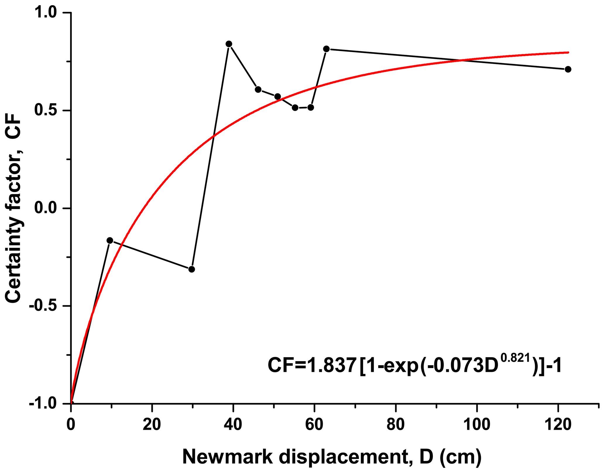
Figure 18CF as a function of Newmark displacement. A dot shows the CF value of a Newmark displacement bin; the red line is the fitting curve of the data using a modified Weibull function.
When fitting the results of shear tests using Coulomb's linear relation, the shear strengths varied widely from high normal stress in the laboratory to low normal stress in the field (Barton, 1973). We introduced the Barton model to the Newmark analysis to reduce the variation in shear strength in terms of Coulomb's constants. We also considered the impact of scale effects by using Eqs. (5) and (6) to prevent Newmark's method from underestimating the shear strength of geological units in regional analysis. In addition, for the Barton model, the joint roughness coefficient (JRC) was estimated from tilt tests, or by matching Barton's joint standard roughness profiles as defined by the International Society for Rock Mechanics (ISRM, 1978). The joint wall compressive strength (JCS) was estimated by Schmidt hammer index tests. These tests helped make a quick estimate of the shear strength in situ, which can facilitate the use of Newmark's method in an emergency hazard and risk assessment after an earthquake.
It is difficult for a statically stable slope to fail under an earthquake. Earthquakes usually cause slopes to fail in the state of limit equilibrium. For this reason, it is important to characterize the shear strength of the slope accurately. The shear strengths were assigned to the geological units using the results of hundreds of shear tests reported in the references provided in Table 1. We assigned the original shear strengths to the geological units, instead of increasing them to render the cells statically stable, as was done by Jibson et al. (1998, 2000). This would have changed the statically stable level of the entire study area, especially the slopes in the state of limit equilibrium. In addition, we considered the size effect of the potential slide surface, which could yield a lower FS and, in turn, a higher displacement. However, the inventory of landslides was used to calibrate the predicted displacements, and the confidence levels indicated by the certainty factors fitted well with the spatial distribution of coseismic landslides, as shown in the hazard map (Fig. 17).
We also ran a conventional Newmark analysis using the assigned strengths, such as friction angle (φ) and cohesion (c), as shown in Table 1. The predicted displacements calculated by the conventional Newmark analysis ranged from 0 to 121 cm, compared with 0 to 122 cm as obtained by the proposed method. Figure 19 shows the hazard map produced using conventional Newmark analysis. The CFs ranged from −1 to 0.94, indicating a very similar result to that of the proposed method above. However, there were large differences along the Shaba River and upstream of the Niulanjiang River between the methods. By comparing Fig. 17 with Fig. 19, we see that the confidence levels of the proposed method fitted the data better than those of the conventional method, especially near upstream portions of the Niulanjiang River. The area under the curve (AUC) was employed to compare the performance of the methods. To create an AUC plot, the cumulative area of CFs within each interval of the calculated values, from the maximum to the minimum, was determined as a proportion of the total study area (x axis) and plotted against the proportion of cumulative landslides falling within those CFs (y axis) (Miles and Keefer, 2009). A value of 0.5 of the AUC indicates that performance is not better than a random guess and that of 1 indicates perfect performance (Miles and Keefer, 2009). Figure 20 shows the results of the AUC analysis of both methods. The calculated value for the proposed method was 0.58 while that for the conventional Newmark's method was 0.53. That is to say, the method introduced here yielded better results and is an improvement over the conventional Newmark analysis.
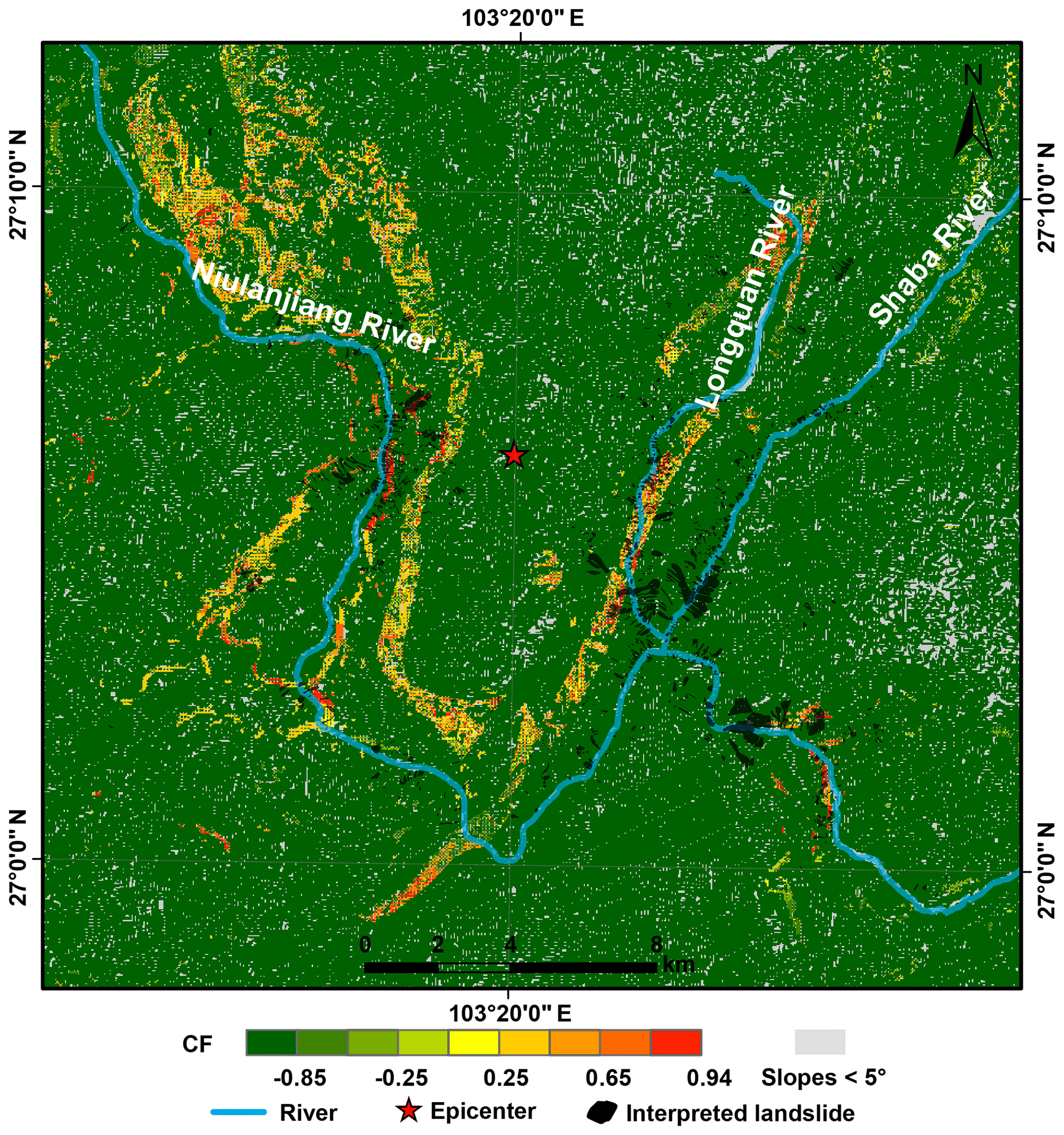
Figure 19Map showing confidence levels of coseismic landslides during the Ludian earthquake using a conventional Newmark analysis. Confidence levels are portrayed in terms of values of CF.
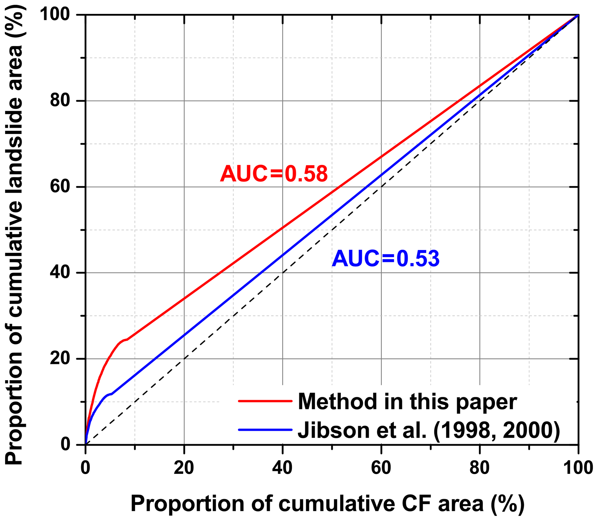
Figure 20Plots of area under the curve comparing the proposed method with the conventional Newmark's method.
Newmark's method is a useful physical model to estimate the seismic stability of natural slopes. The mapping procedure for data on the 2014 Ludian earthquake shows the feasibility of a Newmark analysis combined with Barton's shear strength criterion. Such a method has practical applications in the assessment of regional seismic hazard. We also considered the size effect of parameters of shear strength, such as the joint roughness coefficient (JRC) and the joint wall compressive strength (JCS), in regional analyses. Moreover, linking the Newmark displacements to the certainty factor model improved the utility of Newmark's method to predict the hazard posed by coseismic landslides. Finally, the results of an AUC analysis indicate that the proposed method is more reliable than the conventional Newmark method.
The digital geological map hosted by the China Geological Survey (CGS) can be made available upon request. The pre-earthquake satellite images are available from Google earth, a public desktop software (https://www.google.com/earth/, last access: 30 January 2014). The 0.2 m high-resolution post-earthquake aerial images from the Digital Mountain and Remote Sensing Applications Center, Institute of Mountain Hazards and Environment, Chinese Academy of Sciences, and Beijing Anxiang Power Technology Co., ltd. are restricted and cannot be accessed publicly but may be requested from the corresponding author. The 30 m × 30 m ASTER Global Digital Elevation Model is distributed by NASA EOSDIS Land Processes DAAC (https://doi.org/10.5067/ASTER/ASTGTM.002; NASA/METI/AIST/Japan Spacesystems and U.S./Japan ASTER Science Team, 2009). The dataset of the strong motion stations is provided by the China Earthquake Data Center (http://data.earthquake.cn; China Earthquake Data Center, 2016).
SQ initiated and led this research. MZ designed the analytical framework of this study, produced maps and figures, performed the data analysis and interpretation, and wrote the paper. YZ helped interpret landslides and collect the records of the strong motion stations. SQ, ZS, and BSZ reviewed and edited the paper.
The authors declare that they have no conflict of interest.
This research was supported by the National Natural Science Foundation of China (grant nos. 41825018, 41672307, and 41807273), the Science and Technology Service Network Initiative of the Chinese Academy of Sciences (grant no. KFJ-EW-STS-094), and the China Scholarship Council (grant no. 201704910537).
This research has been supported by the National Natural Science Foundation of China (grant nos. 41825018, 41672307, and 41807273), the Science and Technology Service Network Initiative of the Chinese Academy of Sciences (grant no. KFJ-EW-STS-094), and the China Scholarship Council (grant no. 201704910537).
This paper was edited by Mario Parise and reviewed by two anonymous referees.
Alejano, L. R., González, J., and Muralha, J.: Comparison of different techniques of tilt testing and basic friction angle variability assessment, Rock Mech. Rock Eng., 45, 1023–1035, https://doi.org/10.1007/s00603-012-0265-7, 2012.
Alejano, L. R., Perucho, Á., Olalla, C., and Jiménez, R. (Eds.): Rock engineering and rock mechanics: structures in and on rock masses, CRC Press/Balkema, Leiden, the Netherlands, 1536 pp., 2014.
Ambraseys, N. N. and Menu, J. M.: Earthquake-induced ground displacements, Earthq. Eng. Struct. D., 16, 985–1006, https://doi.org/10.1002/eqe.4290160704, 1988.
Bandis, S., Lumsden, A. C., and Barton, N. R.: Experimental studies of scale effects on the shear behaviour of rock joints, Int. J. Rock Mech. Min., 18, 1–21, https://doi.org/10.1016/0148-9062(81)90262-X, 1981.
Bandis, S. C., Lumsden, A. C., and Barton, N. R.: Fundamentals of rock joint deformation, Int. J. Rock Mech. Min., 20, 249–268, https://doi.org/10.1016/0148-9062(83)90595-8, 1983.
Barton, N.: Review of a new shear-strength criterion for rock joints, Eng. Geol., 7, 287–332, https://doi.org/10.1016/0013-7952(73)90013-6, 1973.
Barton, N. and Bandis, S.: Effects of block size on the shear behavior of jointed rock, in: Proceedings of the 23rd US Symposium on Rock Mechanics (USRMS), Berkeley, California, USA, 25–27 August 1982, 739–760, 1982.
Barton, N. and Choubey, V.: The shear strength of rock joints in theory and practice, Rock Mech., 10, 1–54, https://doi.org/10.1007/BF01261801, 1977.
Bilgin, H. A. and Pasamehmetoglu, A. G.: Shear behaviour of shale joints under heat in direct shear, in: Proceedings of the International symposium on rock joints, Leon, Norway, 4–6 June 1990, 179–183, 1990.
Bray, J. D. and Travasarou, T.: Simplified procedure for estimating earthquake-induced deviatoric slope displacements, J. Geotech. Geoenviron., 133, 381–392, https://doi.org/10.1061/(ASCE)1090-0241(2007)133:4(381), 2007.
Burrough, P. A. and McDonnell, R. A. (Eds.): Principles of geographical information systems (2nd Edition), Oxford University Press, Oxford, UK, 1998.
Chang, Z. F., Chang, H., Yang, S. Y., Chen, G., and Li, J. L.: Characteristics and formation mechanism of large rock avalanches triggered by the Ludian Ms6.5 earthquake at Hongshiyan and Ganjiazhai, Seismol. Geol., 39, 1030–1047, 2017 (in Chinese with English abstract).
Chen, X. L., Ran, H. L., and Yang, W. T.: Evaluation of factors controlling large earthquake-induced landslides by the Wenchuan earthquake, Nat. Hazards Earth Syst. Sci., 12, 3645–3657, https://doi.org/10.5194/nhess-12-3645-2012, 2012.
Chen, X. L., Zhou, Q., and Liu, C. G.: Distribution pattern of coseismic landslides triggered by the 2014 Ludian, Yunnan, China Mw6.1 earthquake: special controlling conditions of local topography, Landslides, 12, 1159–1168, https://doi.org/10.1007/s10346-015-0641-y, 2015.
Chen, X. L., Liu, C. G., Wang, M. M., and Zhou, Q.: Causes of unusual distribution of coseismic landslides triggered by the Mw 6.1 2014 Ludian, Yunnan, China earthquake, J. Asian Earth Sci., 159, 17–23, https://doi.org/10.1016/j.jseaes.2018.03.010, 2018.
Chen, X. L., Liu, C. G., and Wang, M. M.: A method for quick assessment of earthquake-triggered landslide hazards: a case study of the Mw6.1 2014 Ludian, China earthquake, B. Eng. Geol. Environ., 78, 2449–2458, https://doi.org/10.1007/s10064-018-1313-7, 2019.
China Earthquake Data Center: http://data.earthquake.cn, last access: 16 June 2016.
Clough, R. W. and Chopra, A. K.: Earthquake stress analysis in earth dams, ASCE J. Eng. Mech. Div., 92, 197–211, 1966.
Coulson, J. H.: Shear strength of flat surfaces in rock, in: Proceedings of the 13th Symposium on Rock Mechanics, Urbana, Illinois, USA, 30 August–1 September 1971, 77–105, 1972.
Dai, F. C., Xu, C., Yao, X., Xu, L., Tu, X. B., and Gong, Q. M.: Spatial distribution of landslides triggered by the 2008 Ms 8.0 Wenchuan earthquake, China, J. Asian Earth Sci., 40, 883–895, https://doi.org/10.1016/j.jseaes.2010.04.010, 2011.
Geological Engineering Handbook Editorial Committee (Ed.): Geological Engineering Handbook, China Architecture & Building Press, Beijing, China, 2018 (in Chinese).
Giusepone, F. and da Silva, L. A. A.: Hoek & Brown and Barton & Bandis Criteria Applied to a Planar Sliding at a Dolomite Mine in Gandarela Synclinal, in: Proceedings of the ISRM Conference on Rock Mechanics for Natural Resources and Infrastructure-SBMR 2014, Goiania, Brazil, 9–13 September 2014, ISRM-SBMR-2014-009, 2014.
Gu, D. Z. (Ed.): Engineering geomechanics of rock mass, Science Press, Beijing, China, 1979 (in Chinese).
Harp, E. L. and Jibson, R. W.: Landslides triggered by the 1994 Northridge, California, earthquake, B. Seismol. Soc. Am., 86, S319–S332, 1996.
Heckerman, D.: Probabilistic interpretations for MYCIN's certainty factors, Mach. Intell. Patt. Rec., 4, 167–196, https://doi.org/10.1016/B978-0-444-70058-2.50017-6, 1986.
Hoek, E. and Bray, J. D. (Eds.): Rock slope engineering (3rd editon), Taylor & Francis, Abingdon, UK, 1981.
Hsieh, S. Y. and Lee, C. T.: Empirical estimation of the Newmark displacement from the Arias intensity and critical acceleration, Eng. Geol., 122, 34–42, https://doi.org/10.1016/j.enggeo.2010.12.006, 2011.
International Society for Rock Mechanics (ISRM): International society for rock mechanics commission on standardization of laboratory and field tests: Suggested methods for the quantitative description of discontinuities in rock masses, Int. J. Rock Mech. Min., 15, 319–368, https://doi.org/10.1016/0148-9062(78)91472-9, 1978.
Jaeger, J. C. and Cook, N. G. W. (Eds.): Fundamentals of Rock Mechanics, Methuen, London, UK, 513 pp., 1969.
Jibson, R. W.: Predicting earthquake-induced landslide displacements using Newmark's sliding block analysis, Transp. Res. Rec., 1411, 9–17, 1993.
Jibson, R. W.: Regression models for estimating coseismic landslide displacement, Eng. Geol., 91, 209–218, https://doi.org/10.1016/j.enggeo.2007.01.013, 2007.
Jibson, R. W.: Methods for assessing the stability of slopes during earthquakes-A retrospective, Eng. Geol., 122, 43–50, https://doi.org/10.1016/j.enggeo.2010.09.017, 2011.
Jibson, R. W., Harp, E. L., and Michael, J. A.: A method for producing digital probabilistic seismic landslide hazard maps: an example from the Los Angeles, California, area, U.S. Geological Survey, Denver, USA, Open File Rep. 98-113, 17 pp., 1998.
Jibson, R. W., Harp, E. L., and Michael, J. A.: A method for producing digital probabilistic seismic landslide hazard maps, Eng. Geol., 58, 271–289, https://doi.org/10.1016/S0013-7952(00)00039-9, 2000.
Keefer, D. K.: Landslides caused by earthquakes, Geol. Soc. Am. Bull., 95, 406–421, https://doi.org/10.1130/0016-7606(1984)95{\&}amp;lt;406:LCBE{\&}amp;gt;2.0.CO;2, 1984.
Khazai, B. and Sitar, N.: Evaluation of factors controlling earthquake-induced landslides caused by Chi-Chi earthquake and comparison with the Northridge and Loma Prieta events, Eng. Geol., 71, 79–95, https://doi.org/10.1016/S0013-7952(03)00127-3, 2003.
Miles, S. B. and Keefer, D. K.: Evaluation of CAMEL-comprehensive areal model of earthquake-induced landslides, Eng. Geol., 104, 1–15, https://doi.org/10.1016/j.enggeo.2008.08.004, 2009.
NASA/METI/AIST/Japan Spacesystems and U.S./Japan ASTER Science Team: ASTER Global Digital Elevation Model version 002, NASA EOSDIS Land Processes DAAC, https://doi.org/10.5067/ASTER/ASTGTM.002, 2009.
Newmark, N. M.: Effects of earthquakes on dams and embankments, Geotechnique, 15, 139–160, 1965.
Pradel, D., Smith, P. M., Stewart, J. P., and Raad, G.: Case history of landslide movement during the Northridge earthquake, J. Geotech. Geoenviron., 131, 1360–1369, https://doi.org/10.1061/(ASCE)1090-0241(2005)131:11(1360), 2005.
Priest, S. D. (Ed.): Discontinuity analysis for rock engineering, Chapman & Hall, London, UK, 1993.
Qi, S. W., Xu, Q., Lan, H. X., Zhang, B., and Liu, J. Y.: Spatial distribution analysis of landslides triggered by 2008.5.12 Wenchuan Earthquake, China, Eng. Geol., 116, 95–108, https://doi.org/10.1016/j.enggeo.2010.07.011, 2010.
Qi, S. W., Xu, Q., Zhang, B., Zhou, Y. D., Lan, H. X., and Li, L. H.: Source characteristics of long runout rock avalanches triggered by the 2008 Wenchuan earthquake, China, J. Asian Earth Sci., 40, 896–906, https://doi.org/10.1016/j.jseaes.2010.05.010, 2011.
Qi, S. W., Yan, C. G., and Liu, C. L.: Two typical types of earthquake triggered landslides and their mechanisms, in: Proceedings of the 11th International and 2nd North American Symposium on Landslides and Engineered Slopes, Banff, Canada, 3–8 June 2012, 1819–1823, 2012.
Rathje, E. M. and Antonakos, G.: A unified model for predicting earthquake-induced sliding displacements of rigid and flexible slopes, Eng. Geol., 122, 51–60, https://doi.org/10.1016/j.enggeo.2010.12.004, 2011.
Rathje, E. M. and Saygili, G.: Probabilistic assessment of earthquake-induced sliding displacements of natural slopes, Bulletin of the New Zealand Society for Earthquake Engineering, 42, 18–27, https://doi.org/10.5459/bnzsee.42.1.18-27, 2009.
Saygili, G. and Rathje, E. M.: Empirical predictive models for earthquake-induced sliding displacements of slopes, J. Geotech. Geoenviron., 134, 790–803, https://doi.org/10.1061/(ASCE)1090-0241(2008)134:6(790), 2008.
Shortliffe, E. H. and Buchanan, B. G.: A model of inexact reasoning in medicine, Math. Biosci., 23, 351–379, https://doi.org/10.1016/0025-5564(75)90047-4, 1975.
Singh, T. N., Kainthola, A., and Venkatesh, A.: Correlation between point load index and uniaxial compressive strength for different rock types, Rock Mech. Rock Eng., 45, 259–264, https://doi.org/10.1007/s00603-011-0192-z, 2012.
Tang, C., Ma, G., Chang, M., Li, W., Zhang, D., Jia, T., and Zhou, Z.: Landslides triggered by the 20 April 2013 Lushan earthquake, Sichuan Province, China, Eng. Geol., 187, 45–55, https://doi.org/10.1016/j.enggeo.2014.12.004, 2015.
Terzaghi, K.: Mechanism of landslides, in: Application of Geology to Engineering Practice, edited by: Paige, S., Geological Society of America, New York, NY, USA, 83–123, https://doi.org/10.1130/Berkey.1950.83, 1950.
Watson, D. F. and Philip, G. M.: A Refinement of Inverse Distance Weighted Interpolation, Geoprocessing, 2, 315–327, 1985.
Weibull, W. (Ed.): A Statistical Theory of the Strength of Materials, Generalstabens Litografiska Anstalts Förlag, Stockholm, Sweden, 1939.
Wieczorek, G. F., Wilson, R. C., and Harp, E. L.: Map showing slope stability during earthquakes in San Mateo County, California, U.S. Geological Survey, Denver, USA, Map I-1257-E, https://doi.org/10.3133/i1257E, 1985.
Wilson, R. C. and Keefer, D. K.: Dynamic analysis of a slope failure from the 6 August 1979 Coyote Lake, California, earthquake, B. Seismol. Soc. Am., 73, 863–877, 1983.
Xu, C., Xu, X., Zhou, B., amd Yu, G.: Revisions of the M 8.0 Wenchuan earthquake seismic intensity map based on co-seismic landslide abundance, Nat. Hazards, 69, 1459–1476, https://doi.org/10.1007/s11069-013-0757-0, 2013.
Yong, R., Ye, J., Liang, Q. F., Huang, M., and Du, S. G.: Estimation of the joint roughness coefficient (JRC) of rock joints by vector similarity measures, B. Eng. Geol. Environ., 77, 735–749, https://doi.org/10.1007/s10064-016-0947-6, 2018.
Yuan, R.-M., Tang, C.-L., Hu, J.-C., and Xu, X.-W.: Mechanism of the Donghekou landslide triggered by the 2008 Wenchuan earthquake revealed by discrete element modeling, Nat. Hazards Earth Syst. Sci., 14, 1195–1205, https://doi.org/10.5194/nhess-14-1195-2014, 2014.
Zhou, S. H., Chen, G. Q., and Fang, L. G.: Distribution pattern of landslides triggered by the 2014 Ludian earthquake of China: Implications for regional threshold topography and the seismogenic fault identification, ISPRS Int. J. Geo-Inf., 5, 46, https://doi.org/10.3390/ijgi5040046, 2016.