Lagrangian modelling of a person lost at sea during the Adriatic scirocco storm of 29 October 2018

On 29 October 2018 a windsurfer's mast broke about 1 km offshore from Istria during a severe scirocco storm in the northern Adriatic Sea. He drifted in severe marine conditions until he eventually beached alive and well in Sistiana (Italy) 24 h later. We conducted an interview with the survivor to reconstruct his trajectory and to gain insight into his swimming and paddling strategy. Part of survivor's trajectory was verified using high-frequency radar surface current observations as inputs for Lagrangian temporal back-propagation from the beaching site. Back-propagation simulations were found to be largely consistent with the survivor's reconstruction. We then attempted a Lagrangian forward-propagation simulation of his trajectory by performing a leeway simulation using the OpenDrift tracking code using two object types: (i) person in water in unknown state and (ii) person with a surfboard. In both cases a high-resolution (1 km) setup of the NEMO v3.6 circulation model was employed for the surface current component, and a 4.4 km operational setup of the ALADIN atmospheric model was used for wind forcing. The best performance is obtained using the person-with-a-surfboard object type, giving the highest percentage of particles stranded within 5 km of the beaching site. Accumulation of particles stranded within 5 km of the beaching site saturates 6 h after the actual beaching time for all drifting-particle types. This time lag most likely occurs due to poor NEMO model representation of surface currents, especially in the final hours of the drift. A control run of wind-only forcing shows the poorest performance of all simulations. This indicates the importance of topographically constrained ocean currents in semi-enclosed basins even in seemingly wind-dominated situations for determining the trajectory of a person lost at sea.

1 Introduction

Lagrangian particle tracking of objects lost at sea is an important branch of ocean forecasting. Maritime search and rescue (SAR) or other types of civil service responses depend on timely and reliable estimates of the most probable areas which contain the drifting object. These estimates generally require prior computation of ocean currents, waves, and winds in the area, which are most often provided by numerical circulation, wave, and atmosphere models.

The wind force contribution to the object's drift is termed its leeway and has both downwind (drag) and crosswind (lift) components (Breivik and Allen, 2008). The object's drift therefore generally deviates from the wind direction by some divergence angle (Allen and Plourde, 1999), related to the downwind and crosswind components. Specific values of the object's downwind and crosswind drift are determined by the balance of the wind (lift and drag) force on the overwater part of the object and the hydrodynamic (lift and drag) force on the subsurface part of the object – the object's drifting properties therefore depend significantly on its shape. Empirical observations have consequently been the most straightforward method of determining the drifting parameters for various drifting object types, including human bodies (Allen and Plourde, 1999; Hackett et al., 2006). Reports on marine drifts involving survivors are not ubiquitous, which makes reviews like the one from Allen and Plourde (1999) all the more valuable for modelling marine drifts of persons or other objects.

In this paper we focus on an incident which occurred on 29 October 2018 in the northern Adriatic Sea and led to a 24 h drift of a person in gale wind conditions (level 8 on Beaufort scale). For an extensive analysis of the atmospheric and marine conditions during the 29 October 2018 storm the reader is referred to Cavaleri et al. (2019). These conditions are related to the fact that the Adriatic Sea is a northwest–southeast-oriented elongated basin of the northern central Mediterranean, exchanging properties with the eastern Mediterranean basin through the Otranto Strait (40^∘ N, 19^∘ E, in Fig. 1a). It is 800 km long and 200 km wide and surrounded on all sides by mountain ridges – the Alps in the north, the Apennines in the west, and the Dinaric Alps in the east. These ridges exhibit significant influence on the basin circulation through topographic control of the airflow, most notably during episodes of the northeasterly bora wind and southeasterly scirocco. The northern part of the Adriatic is a shallow shelf with depths under 60 m. Its northernmost part, extending into the Gulf of Trieste, is the shallowest, with depths around 20 to 30 m (see Fig. 1b).

In the afternoon of 29 October 2018, the scirocco speeds along the west coast of northern Istria were in the range of 15–25 m s⁻¹, and significant wave heights amounted to 3–5 m (Cavaleri et al., 2019), while maximum wave heights in the southern part of the Gulf of Trieste at coastal buoy Vida (see Sect. 2.1 for details and Fig. 1b for location) were observed to be over 2.5 m (not shown). The town of Umag in northern Istria is a popular windsurfing spot during scirocco conditions: on 29 October 2018 many people were windsurfing there when the accident occurred at around 16:00 UTC. The windsurfer's mast broke roughly 1 km offshore northwest of Umag (see Fig. 1b for location) initiating the drift. The conditions were too severe for immediate marine rescue either by his colleagues or by authorities. The surfer beached on his own 24 h later close to Sistiana north of Trieste (see Fig. 1b). The windsurfer's harness was however recovered in the central part of the Gulf of Trieste at around 15:00 UTC on 30 October.

The survivor kindly responded to our interview request. He is an experienced windsurfer and has been windsurfing along the coasts of Gulf of Trieste for the past 30 years. We state that explicitly to convey the fact that he knows this coastline very well. We now briefly recapitulate his personal statements about the drift. He was conscious and focused the entire time. The visibility was not bad and he could see the coastline of the Gulf of Trieste in its entirety, which helped him make mental notes of his location. He was highly alert to his location throughout the drift but did not have a watch or a GPS. We have therefore attempted to independently validate his trajectory estimate, as will be explained below in Sect. 4.1.

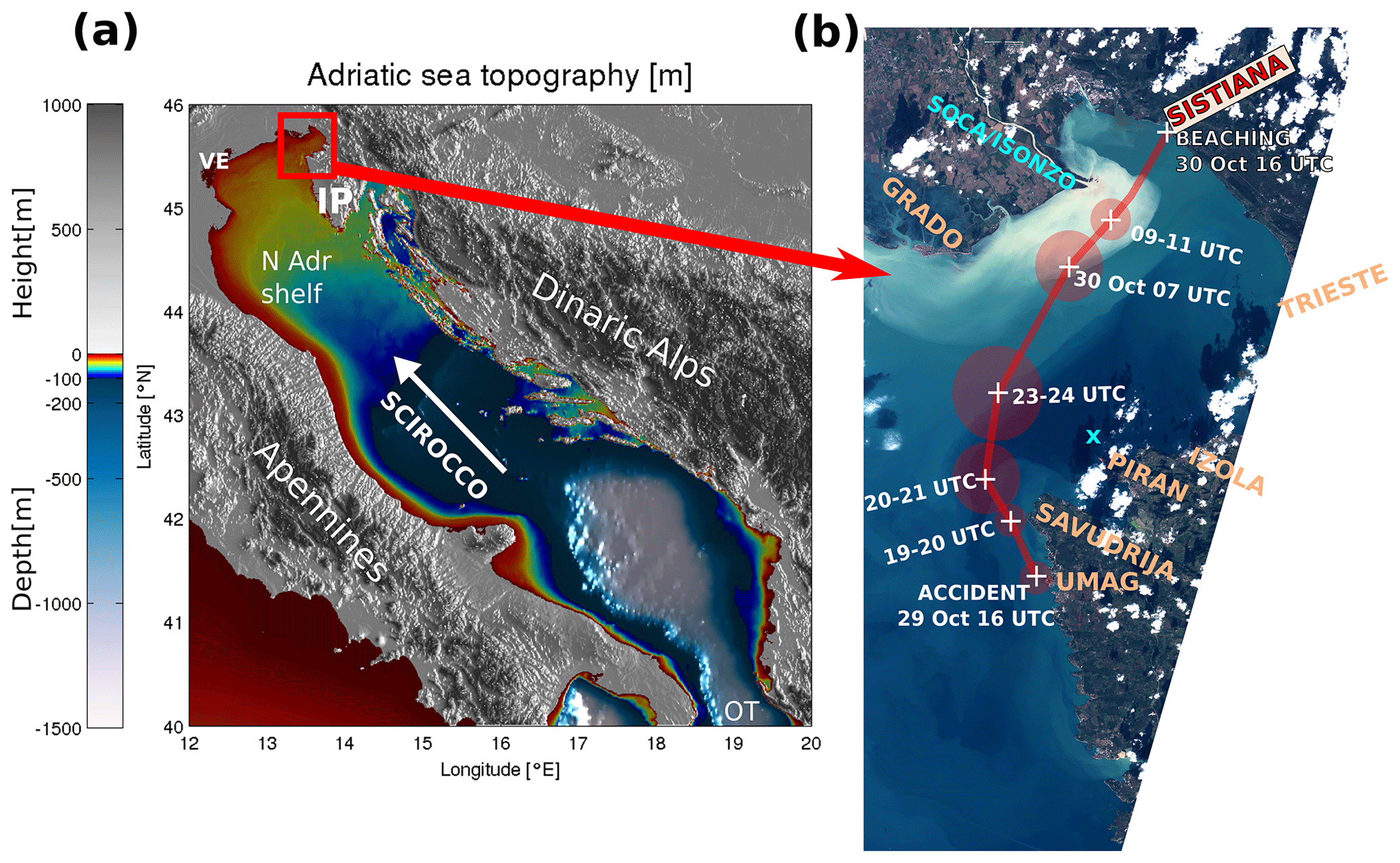
Figure 1 (a) Adriatic basin bathymetry. Abbreviations are as follows: VE – Venice; IP – Istrian Peninsula; N Adr Shelf – northern Adriatic Shelf; OT – Otranto Strait. The direction of the scirocco is marked with a white arrow. (b) The Gulf of Trieste and piecewise trajectory of the drift as estimated by the survivor. Location estimates are junctions of the piecewise straight line. Circles denote location uncertainty estimates at specific times. The cyan “X” sign north of Piran denotes the location of the Vida coastal buoy. The background layer is a Sentinel-2 L1C true colour image of the Gulf of Trieste from the day after the beaching, 31 October 2018 (obtained from Copernicus Open Access Hub: https://scihub.copernicus.eu, last access: 19 August 2020). The turbid Soča River plume is clearly visible along the northern shore of the Gulf.

His mast broke on 29 October 2019 16:00 UTC at 45.558^∘ N, 13.625^∘ E, with an estimated ±500 m error in each direction; see Fig. 1b for location. Immediately after the accident, he drifted alongshore north of Umag and he actively paddled towards the coast, hoping to reach the Cape of Savudrija. The wind direction at his location was however slightly offshore, and sometime between 19:30 and 20:30 UTC he realized he would not be able to reach Savudrija. After 20:00 UTC the scirocco strengthened. He was then located northwest of Savudrija, drifting north-northwest toward Grado. Swimming was not possible due to air spray and sea conditions, but he kept shaking his arms and legs interchangeably to keep warm. At some point between 20:00 and 23:00 UTC he could see the town of Izola (Slovenia) and the town of Grado (Italy) at right angles. It was around 23:00 UTC that his drift turned northeast. After 23:00 UTC, he was located approximately on the Piran-Grado line. Sea conditions became very severe. He was laying on the surfboard, mostly facing southwest, away from the mean drift direction, drifting backwards, clutching the foot straps on the surfboard. He estimates that every 50th wave broke over him and pulled the surfboard from under him. When this happened he needed to wait to reach the crest of the wave to visually re-locate the board and catch it. In the morning, on 30 October 2018 07:00 UTC, he was located 2–4 km south-southwest of the Soča (also known as the Isonzo) River mouth. By 09:00–10:00 UTC he was located roughly 1–2 km south-southeast of the river mouth, and the water became significantly colder as he likely entered the Soča River plume (visible in Fig. 1b). By the time he entered the plume, the Soča runoff was at a several-month maximum, as depicted in Fig. 2. From 11:00 UTC on he paddled actively toward the northeast to overcome the riverine westward coastal current until he reached the beach near Sistiana at 16:00 UTC.

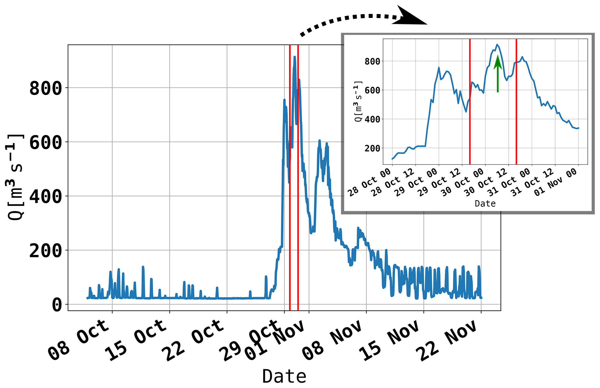
Figure 2 Soča runoff during October and November 2018, as measured at an upstream river gauge (operated by ARSO) at Solkan, Slovenia. Vertical red lines indicate the time window of the drift. The green arrow in the inset marks the approximate time of the windsurfer's entering the river plume.

The drifting trajectory, reconstructed from above, is shown in Fig. 1b. Due to the nature of the testimony and lack of measuring equipment, the survivor's trajectory is burdened with error. The survivor estimated the errors in his spatio-temporal location to the best of his ability: these estimates, arbitrary as they are, are presented as semi-transparent circles around each marked location in Fig. 1 and other figures. We have however attempted to verify the final part of his trajectory by using high-frequency radar surface current measurements (see Sect. 4.1). High-frequency (HF) measurements do not cover the entire area of the drift, but they do cover the final half of the drift. We could therefore not use HF observations to force the survivor's drift from start to finish, but we could use them to perform Lagrangian back-propagation of particles from his beaching location back into the gulf. As will be shown later, these results are consistent with the survivor's trajectory estimate. While not allowing for any meaningful quantitative verification of the Lagrangian codes in this paper, we believe that the trajectory is a qualitatively suitable guide for our simulations.

In the present paper, we present two attempts to simulate this trajectory using the state-of-the-art particle tracking model OpenDrift. Available observations and general marine conditions during the drift are presented in Sect. 2; numerical models used for the particle tracking modelling chain are described in Sect. 3. The Lagrangian model OpenDrift and its setup are presented in Sect. 3.2. Simulation results are depicted and discussed in Sect. 4, followed by concluding remarks in Sect. 5.

2 Observations

2.1 Coastal buoy Vida

The oceanographic buoy Vida is a coastal observation platform, operated by the Marine Biology Station at the National Institute of Biology (NIB). It is located in the southern part of the Gulf of Trieste at (45.5488 ^∘N, 13.55505 ^∘E); see Fig. 1b (marked with a cyan cross). Data from the buoy are multifaceted (air temperature, air humidity, currents, waves, sea temperature, salinity, dissolved oxygen, chlorophyll concentration, etc.) and are publicly available (http://www.nib.si/mbp/en/buoy/, last access: 19 August 2020) in near-real time. Ocean currents are acquired by a Nortek AWAC acoustic Doppler current profiler, mounted on the sea bottom at a depth of 22.5 m, to monitor vertical current profiles (at 1 m intervals along the water column). The topmost cell of the ADCP measurement corresponds to a depth around 0.5 m. Further information on the buoy can be found in Malačič (2019).

2.2 High-frequency radar system

The HF systems deployed in the Gulf of Trieste consist of two WERA stations (Gurgel et al., 1999) manufactured by Helzel Messtechnik in Germany, one at the OGS facility in Aurisina (Italy) and the second, operated by NIB, in the urban area of Piran (Slovenia). The systems have provided sea surface current maps since January 2015. They rely on the scattering of a short-duration (9 min) and low-power (below 20 W) harmless radio wave pulses from waves at the ocean surface satisfying the Bragg-resonance scattering condition for coherent return. The two systems operate at a carrier frequency of 25.5 MHz as regulated by the International Telecommunication Union, covering the Gulf of Trieste at 1 km range resolution and 1^∘ angular resolution every 30 min. After acquisition, data are processed and radial components of the surface current field are obtained, which in turn are combined into a 1.5 km horizontal resolution 22 × 20 regular grid (see Fig. 3 for coverage during the event and both station locations). Combined data are stored in databases and can be visualized in near real time at http://www.nib.si/mbp/en/oceanographic-data-and-measurements/other-oceanographic-data/hf-radar-2 (last access: 19 August 2020). WERA system external antenna field calibration was performed in 2016, and WERA system intrinsic estimates of zonal and meridional current errors amount to 1–3 cm s⁻¹ (roughly 3 %–10 % of observed current speed) during the period of the drift. Data availability during the 24 h of the drift was between 50 % and 70 %, as depicted in Fig. 3. The strip without data, visible in Fig. 3 along the connecting line between the two WERA systems, occurs due to geometric dilution of precision: along the connecting line, the two radar stations measure exactly the same radial current components from which no reconstruction of transverse current components can be made. Lacking transverse information, no estimate of the total current can be made along this line. The two WERA HF systems are operated and maintained in collaboration between researchers, engineers, and technicians from OGS and NIB.

3 Models

3.1 Ocean and atmospheric models

3.1.1 NEMO circulation model

We are using a high-horizontal-resolution ($\mathrm{1}{}^{\circ }/\mathrm{111}$ or roughly 1000 m) setup of NEMO v3.6 (Madec, 2008) over the Adriatic basin on a regular 999×777 longitude–latitude grid and 33 vertical z^* levels with a partial step. The model domain spans 12–21^∘ E and 39–46^∘ N; see Fig. 3. Maximum vertical discretization stretch is located at the 15th level to allow for appropriate vertical resolution near the surface. In all regions shallower than 2 m, a minimum 2 m depth is enforced. Vertical level depths in metres are 0.50, 1.51, 2.55, 3.64, 4.83, 6.20, 7.94, 10.38, 14.18, 20.56, 31.68, 51.23, 84.58, 137.94, 215.83, 318.24, 440.67, 576.90, 721.55, 870.95, 1022.92, 1176.25, 1330.29, 1484.69,1639.28, 1793.97, 1948.71, 2103.47, 2258.25, 2413.03, 2567.81, 2722.60, and 2877.39. Explicit time splitting is enforced, and barotropic time step is automatically adjusted to meet the Courant–Friedrichs–Lewy stability criterion. The baroclinic time step was set to 120 s. The model runs daily at the Slovenian Environment Agency (ARSO). It is initialized from previous operational runs. Hourly lateral boundary conditions in the Ionian Sea are taken from the Copernicus CMEMS MFS model. Turbulent heat and momentum fluxes across the ocean surface are computed with the CORE bulk flux formulation (Large and Yeager, 2004) using ALADIN SI atmospheric fields (surface wind, longwave and shortwave radiation fluxes, mean sea level pressure, 2 m temperature, specific humidity, and precipitation). Rivers are implemented as freshwater release over the entire water column at the discharge location, with runoff values as described in Ličer et al. (2016). Tides are included as lateral boundary conditions for open boundary elevations and barotropic velocities for K1, P1, O1, Q1, M2, K2, N2, and S2 constituents. Constituents at the open boundary are obtained using OTIS tidal inversion code (Egbert and Erofeeva, 2002), based on the TPXO8 atlas. The model employs Flather boundary conditions for barotropic dynamics and a flow relaxation scheme (Engedahl, 1995) for baroclinic dynamics and tracers at the open boundary. Lateral momentum boundary conditions at the coast are free-slip. Bottom friction is nonlinear with a logarithmic boundary layer. Lateral diffusion schemes for tracers and momentum are both bi-Laplacian over geopotential surfaces. Vertical diffusion is computed using a generic length scale (GLS) turbulence scheme. The Craig and Banner formulation (Craig and Banner, 1994) of surface mixing due to wave breaking is switched on. The present NEMO setup does not have data assimilation and all the simulations in this paper consequently lack any data assimilation as well.

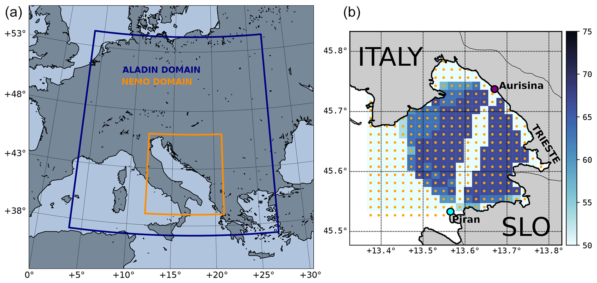
Figure 3 (a) Computational domains of ALADIN SI (blue) and NEMO (orange) numerical models. (b) WERA HF radar grid (orange dots) and data availability percentage per grid point between 29 October 2018 16:00 UTC and 30 October 2018 21:00 UTC.

3.1.2 ALADIN atmospheric model

The version of the model used for the experiments in this paper is currently operational at the Slovenian Weather Service. It runs on a 432×432 horizontal Lambert conic conformal grid with 4.4 km resolution and 87 vertical levels with the model top at 1 hPa and a model integration time step of 180 s. The model domain spans [0.7^∘ W, 28.6^∘ E] in longitude and [37.4^∘ N, 55.0^∘ N] in latitude; see Fig. 3. The physics package used in the model is the so-called ALARO-0, which uses the Modular, Multi-scale, Microphysics and Transport (3MT) structure (Gerard et al., 2009). Initial conditions for the model are provided by atmospheric analysis with 3-hourly three-dimensional variational assimilation (3D-Var) (Fischer et al., 2005; Strajnar et al., 2015) and optimal interpolation for surface and soil variables. Sea surface temperature (SST) in the model is initialized from the most recent host model analysis of the ECMWF model that uses Operational Sea Surface Temperature and Sea Ice Analysis (OSTIA; Donlon et al., 2012), supplied by the National Environmental Satellite, Data and Information Service (NESDIS) of the American National Ocean and Atmospheric Administration (NOAA). Information at the domain edge is obtained from the global model by applying Davies relaxation (Davies, 1976). Lateral boundary conditions are provided by the ECMWF Boundary Conditions Optional project and are applied with a 1 h period in the assimilation cycle and a 3 h period during model forecasts. Boundary condition information is interpolated linearly for time steps between these times. Further details about the model setup and assimilation scheme are available in Strajnar et al. (2015, 2019) and Ličer et al. (2016).

3.2 Lagrangian models and OpenDrift setup

Lagrangian or particle tracking models are used for general purpose tracking problems from marine oil-spill dispersion modelling to water age, marine bacterial transport, and object drift forecasting. Typically an arbitrary number of particles N_p (i.e. several thousand) are seeded at the initial location and subjected in each time step to advection, turbulent diffusion, and, if applicable, fate. Throughout this paper all the particles are considered passive; i.e. their advection is solely due to external forcing from wind and sea. Lagrangian trajectory r_p(t) of the pth particle ($p=\mathrm{1},\mathrm{\dots },N_{\mathrm{p}}$) is computed using a suitable numerical method (i.e. Runge–Kutta or Euler method) to integrate the following initial value problem:

$$\begin{array}{}\text{(1)}& {\displaystyle \frac{\mathrm{d}{\mathbf{r}}_{\mathrm{p}}}{\mathrm{d}t}}& {\displaystyle }={\mathbf{u}}_{\mathrm{c}}({\mathbf{r}}_{\mathrm{p}},t)+{\mathbf{l}}_{\mathrm{p}}({\mathbf{r}}_{\mathrm{p}},t)+{\mathbf{u}}_{\mathrm{s}}({\mathbf{r}}_{\mathrm{p}},t),\text{(2)}& {\displaystyle }{\mathbf{r}}_{\mathrm{p}}{|}_{t=\mathrm{0}}& {\displaystyle }={\mathbf{r}}_{\mathrm{0},\mathrm{p}},\end{array}$$

where t denotes time, and r_0, p in Eq. (2) denotes initial position of the pth particle.

Terms of the right-hand side of Eq. (1) are as follows. Term u_c(r_p, t) denotes the Eulerian ocean current at particle location r_p(t) at time t. In this study this term is obtained from the NEMO circulation model (Sect. 3.1.1) for forward propagation simulations or from WERA HF radar observations for back-propagation simulations (Sect. 4.1). Term l_p(r_p, t) denotes leeway of the pth particle at particle location r_p at time t. The leeway term is computed from ALADIN winds (Sect. 3.1.2) as follows. Due to lift forces on the drifting object, its leeway is not oriented strictly downwind but has a crosswind component as well or $\mathbf{l}=(l_{\parallel },l_{⟂})$, where l_∥ and l_⟂ are downwind and crosswind leeway components respectively. Experimental data however suggest an almost linear relationship between wind speed and downwind and crosswind leeway components (Breivik and Allen, 2008). Therefore the downwind leeway component can be parameterized as $l_{\parallel }=a_{\parallel }{u}_{\mathrm{10}}+b_{\parallel }$, where u₁₀ denotes wind speed. On the other hand the crosswind force can point both to the left and to the right of wind, depending on the orientation and shape of the object in the wind field. Therefore crosswind leeway degenerates into left-drifting crosswind leeway component $l_{⟂}^{\mathrm{L}}=a_{⟂}^{\mathrm{L}}{u}_{\mathrm{10}}+b_{⟂}^{\mathrm{L}}$ and a right-drifting crosswind leeway component $l_{⟂}^{\mathrm{R}}=a_{⟂}^{\mathrm{R}}{u}_{\mathrm{10}}+b_{⟂}^{\mathrm{R}}$. Coefficients $(a_{\parallel },b_{\parallel })$, $(a_{⟂}^{\mathrm{L}},b_{⟂}^{\mathrm{L}})$, and $(a_{⟂}^{\mathrm{R}},b_{⟂}^{\mathrm{R}})$ are determined from observations as a least-square linear fit between observed wind velocity and observed leeway vector (Breivik and Allen, 2008; Allen and Plourde, 1999). The coefficients $(a_{⟂}^{\mathrm{L}},b_{⟂}^{\mathrm{L}})$ and $(a_{⟂}^{\mathrm{R}},b_{⟂}^{\mathrm{R}})$ are similar but not identical. This linear regression also yields downwind, left-drift, and right-drift standard deviations for each fit.

Term u_s(r_p, t) on the right-hand side of the Eq. (1) is the Stokes drift contribution, i.e. mean shift of a fluid particle due to unclosed Lagrangian orbit of the particle in the gravity wave field. Note however that since coefficients $(a_{\parallel },b_{\parallel })$ and $(a_{⟂},b_{⟂})$ are determined from observations, they already contain the Stokes drift contribution of the local wind sea in the observed leeway. In our attempt to model the object's leeway using downwind and crosswind leeway coefficients based on empirical data from Allen and Plourde (1999), we have omitted the Stokes drift term from the initial value problem (Eqs. 1–2), as explained in Breivik and Allen (2008).

OpenDrift is an open-source Python-based Lagrangian particle modelling code developed at the Norwegian Meteorological Institute with contributions from the wider scientific community. Its Leeway module implements leeway computation in the fashion described in the previous paragraph; for further details see Breivik and Allen (2008) and Dagestad et al. (2018). Apart from leeway computations OpenDrift supports a wide range of offline (i.e. with precomputed currents and winds) predictions from oil spills and drifting objects to microplastics and fish larvae transport. Particle seeding is very convenient to use and its Leeway module supports a wide range of object types with different lift and drag behaviour under current and wind forces (Dagestad et al., 2018).

The object types used in this study were of two kinds that we believe are most adequate for leeway modelling in this particular case. The first drift object type was “person in water”, corresponding to an empirically determined (Allen and Plourde, 1999) downwind slope of $a_{\parallel }=\mathrm{1.93}\mathit{\%}$, downwind standard deviation of 0.083 ms⁻¹, right slope of $a_{⟂}^{\mathrm{R}}=\mathrm{0.51}\mathit{\%}$, right standard deviation of 0.067 ms⁻¹, left slope of $a_{⟂}^{\mathrm{L}}=-\mathrm{0.51}\mathit{\%}$, and left standard deviation of 0.067 ms⁻¹.

The second object type was “person-powered vessel 2” (person with a surfboard), corresponding to an empirically determined (Allen and Plourde, 1999) downwind slope of $a_{\parallel }=\mathrm{0.96}\mathit{\%}$, downwind standard deviation of 0.12 ms⁻¹, right slope of $a_{⟂}^{\mathrm{R}}=\mathrm{0.54}\mathit{\%}$, right standard deviation of 0.094 ms⁻¹, left slope of $a_{⟂}^{\mathrm{R}}=-\mathrm{0.54}\mathit{\%}$, and left standard deviation of 0.067 ms⁻¹.

The simulation was run in both cases for 48 h using a second-order Runge–Kutta scheme. Forcing data consisted of NEMO currents and ALADIN SI 10 m winds from the 00:00 UTC operational runs of both models, performed on 29 October 2018 at ARSO.

At the time of the incident, however, OpenDrift was not implemented at ARSO and could not be used. Due to the incident, the pipeline of input data preparation and a specific drifting-particle-type OpenDrift computation was developed and is now available to forecasters at ARSO as an internal web service. With ALADIN SI and NEMO fields (pre)computed operationally, subsequent on-demand OpenDrift simulations take under 10 min to complete.

4 Results and discussion

4.1 Drift trajectory verification: comparison of the survivor's trajectory to backtracking estimates from HF radar

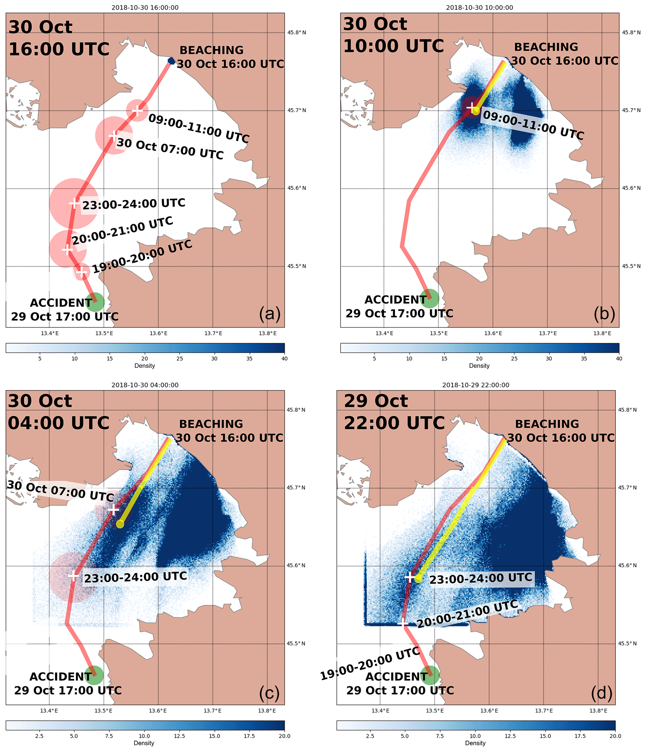
Figure 4 Temporal back-propagation of virtual particles from the beaching location using HF radar measurements and ALADIN winds as inputs for the OpenDrift model. Back-propagation starts at the beaching location (a). Particle spatial density is shown every 6 h of the simulation, as denoted by timestamps in the top left corner of each panel. The red line and superimposed dates are the survivor's estimates of his trajectory (for clarity, only relevant time steps of the survivor's reconstruction are shown in each panel). Transparent red circles denote the survivor's estimate of the error in his location at the stated time. The yellow line is a reconstruction of the survivor's trajectory from back-propagation simulations. Dark blue straight lines in (d), appearing along the southwest corner of HF radar computational domain, result from accumulation of particles which cease to advect when they reach the outer limits of the HF radar domain.

As noted above, the survivor had no GPS or watch to keep track of his movements in space and time. Therefore his reconstruction of the drift trajectory is burdened with error. What is known however is the exact location and time of his beaching: a beach in Sistiana (Italy) on 30 October 2018 at 16:00 UTC. HF radar surface current measurements cover only the final part of the drift domain. They can therefore, in themselves, not be used for a full forward-propagation simulation (starting at the accident location and ending at the beaching location), but they can nevertheless be employed to perform Lagrangian back-propagation (upwind and upstream advection backwards in time) during the final part of the drift.

Such a simulation is of course limited to the HF system domain, described in Sect. 2.2, but it should offer some insight into the final part of the drift trajectory and serve as an independent check of the survivor's trajectory estimate. To this end, HF radar currents over the period of the drift were first gap-filled in space using nearest-neighbour interpolation and then gap-filled in time using linear interpolation. The wind component for back-propagation was provided by the ALADIN atmospheric model (see Sect. 3.1.2) and remapped to the HF radar grid in space and time. OpenDrift code was used to perform back-propagation simulation, and results are presented as particle numeric density per area, in a similar fashion as in Röhrs et al. (2018) and Dugstad et al. (2019). To ensure smooth maps of particle density, a large number (50 000) of virtual particles of the type person with a surfboard were released from a circle within a 500 m radius from the beaching location at beaching time. Particles were then advected backward in time in 12 min time steps (0.2 h) for 18 h. Results of these simulations are depicted in Fig. 4, which shows particle density per density cell area. Density cells over which the particles are counted were chosen to be of 150 m×150 m dimensions. This 10-fold reduction in cell computation area was done because the original HF radar grid (1500 m×1500 m; see Fig. 3) is too coarse to produce smooth maps of particle density.

Figure 4 indicates two distinct pathways to Sistiana during the time of the drift: firstly we have the southern branch arriving to the beaching site from the region south-southeast of the beaching site. Since we know that the survivor drifted into the gulf from outside of the gulf, and not from the region south-southeast of the beaching site, this pathway is not significant for our analysis. Secondly, a northwestern branch of propagation is marked with a yellow line in Fig. 4 and extends roughly along the survivor's trajectory estimate. This pathway is qualitatively (spatially and temporally) consistent with the survivor's trajectory. The survivor's estimates of his location on 29 October 22:00 UTC and 30 October 10:00 UTC agree well with the computed virtual particle density maps. During the night, when the survivor reported feeling maximum distress, the back-propagation estimate of trajectory is located 2–4 kilometers to the east of his reconstruction.

Additional back-propagation simulation was performed with NEMO-modelled currents in an identical fashion as described above. This allows for a comparison with back-propagation due to the HF currents. This simulation is not shown here but is depicted in Fig. S1 in the Supplement. It indicates that NEMO currents tended to underestimate observed currents throughout the drift. This underestimation is however most notable in the final hours of the drift, as also stated below in Sect. 4.2 and 4.3.

4.2 Marine conditions from observations and models

In this section we present a qualitative analysis of marine conditions from available observations and also marine drift results from both particle tracking models presented in Sect. 3.2.

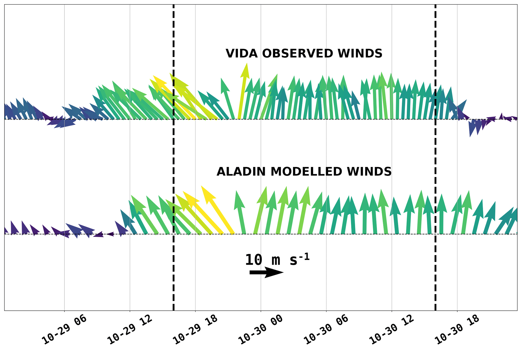
Figure 5 Arrow plots of observed and ALADIN SI modelled wind directions at the Vida coastal buoy during the 29 October 2018 event. The drift period is marked with dashed vertical lines. Arrows are coloured by their wind speed.

Figure 5 depicts wind measurements and ALADIN SI modelled winds at the Vida coastal buoy (12 km northeast of the accident location; see Fig. 1b) for the time window 29–31 October 2018. Qualitatively there is a very solid agreement between the two time series. Measured wind at Vida exhibits a southeasterly 140^∘ direction in the hours after the accident (left dashed line in Fig. 5), followed by a shift to slight south-southwest 190^∘ between 30 October 00:00 and 04:00 UTC, and finally a southerly 180^∘ direction during the day (all directions in the paper are stated in nautical notation, i.e. 0^∘ marking north, 90^∘ marking east). Wind speed is constantly around 15–20 ms⁻¹.

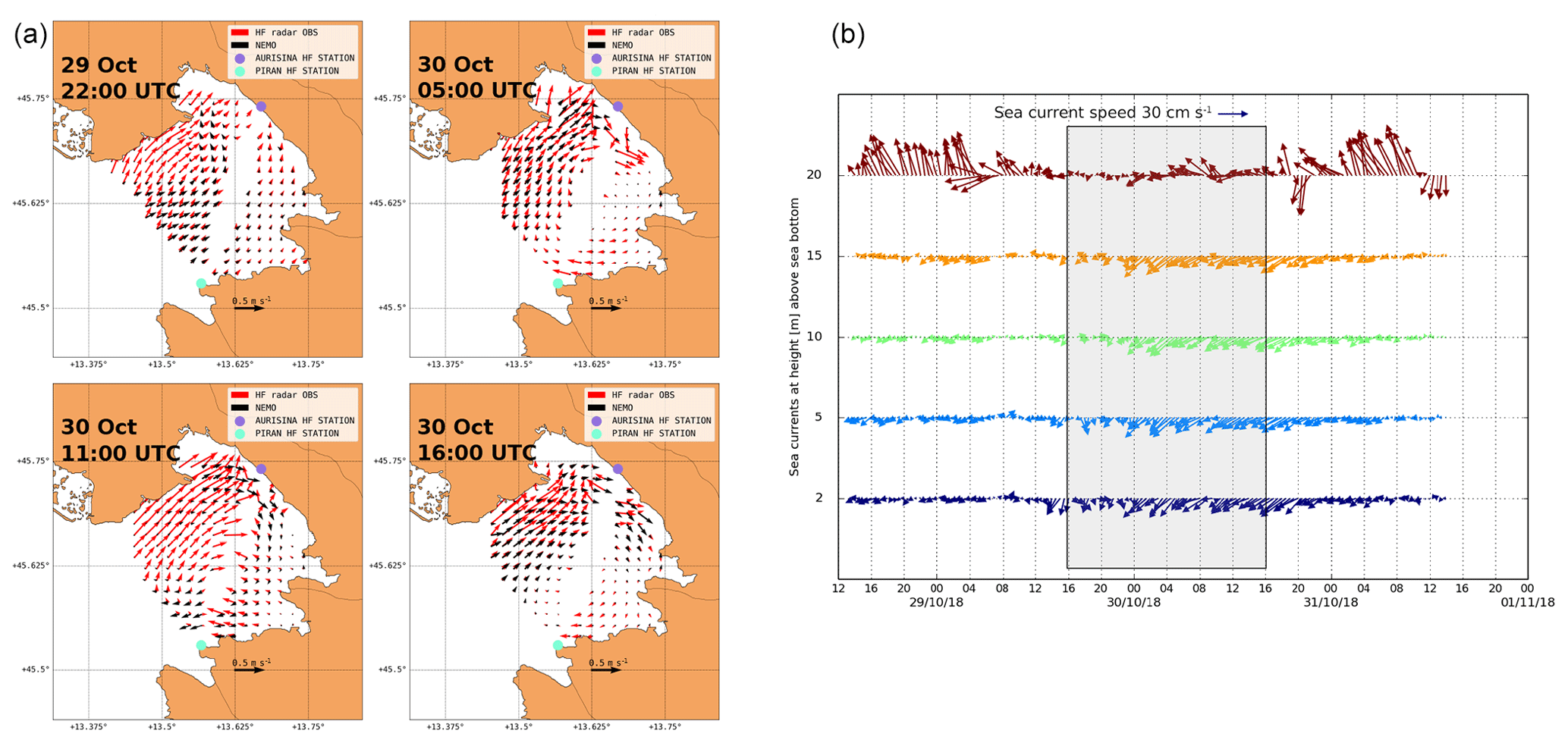
Figure 6 (a) HF radar measurements in the Gulf of Trieste during the period of the drift. Since there are gaps in surface current measurements, the closest observations to 29 October 22:00 UTC and 30 October 04:00, 10:00, and 16:00 UTC are depicted. NEMO currents were bilinearly interpolated to WERA grid points. Arrow lengths from both fields are commonly scaled. (b) Arrow plot of ADCP measurements of ocean currents at the Vida coastal buoy during the 29 October 2018 event (shaded rectangle delimits the time window of the drift). Surface current time series is plotted in the top line.

HF observations in Fig. 6 are presented as a qualitative check for the NEMO model surface currents during the 24 h of the drift. HF measurements and modelled currents both exhibit eastward topographically constrained coastal current in the northern part of the gulf between Grado and the Soča River mouth, with the NEMO model tending to misrepresent and underestimate observations (as shown below however, wind drift was the main contribution to the drift). Absence of the coastal current on 29 October 22:00 UTC might be related to the model treatment of high Soča discharge, which in itself generates westward inertial current in that part of the modelling domain and might be counteracting wind-driven (eastward) currents. Verification of the NEMO model versus 10 months of hourly HF radar currents (not shown in detail in this paper) yields daily averages of bias in zonal velocity $<u_{\mathrm{NEMO}}-u_{\mathrm{HF}}{>}_{\mathrm{24}\mathrm{h}}$ between 0 and −2.5 cm s⁻¹ and a daily averaged bias for meridional velocity $<v_{\mathrm{NEMO}}-v_{\mathrm{HF}}{>}_{\mathrm{24}\mathrm{h}}$ between +2.5 and −2.5 cm s⁻¹. The NEMO model underestimations during the limited period of this case study were unfortunately much larger: spatially averaged (over the HF domain) and temporally averaged (over the period of the drift) NEMO biases amounted to −8.3 cm s⁻¹ for zonal velocity and a bias of −8.8 cm s⁻¹ for meridional velocity. Focusing on the period of the drift, NEMO model performance was best in the beginning and worst at the end of the drift. Over the first 18 h of the drift, the NEMO model exhibited −8.2 (8.1) cm s⁻¹ bias in zonal (meridional) velocity, while during the last 6 h of the drift these biases amounted to $-\mathrm{11.4}(-\mathrm{11.1})$ cm s⁻¹. Additional forward-tracking simulations were also performed to compare advection due to HF and NEMO currents. These simulations are not included here but are described and depicted in Fig. S2. They indicate that most of the error due to NEMO current underestimation was accumulated in the final hours of the drift. This performance will have to be further addressed as a separate issue and needs to be kept in mind when interpreting results below. On the other hand both the model and the HF measurements exhibit an inflow over most of the surface area of the gulf, which indicates that the surface layer on 29 October 22:00 UTC was wind dominated; see also Malačič et al. (2012).

Another common feature of NEMO currents and HF radar observations is the general anticyclonic character of the surface circulation through the rest of the night and the following day. This is in contrast with the northern Adriatic basin-scale cyclonic current pattern during scirocco episodes (not shown) and stems from the fact that scirocco-induced surface currents, flowing north along the Istrian coast, typically branch upon hitting the northern end of the Adriatic basin. The eastward branch of this wind-driven current inflows into the Gulf of Trieste along the northern coastline. Such inflow, visible in modelled and observed currents, is therefore not unexpected during scirocco episodes. As is further shown in Fig. 6b, in situ currents measured at the Vida buoy also exhibit a westward direction over the entire water column during the time window of the drift and are therefore consistent with the overall anticyclonic character of the surface circulation, exhibited in the model and radar surface current maps.

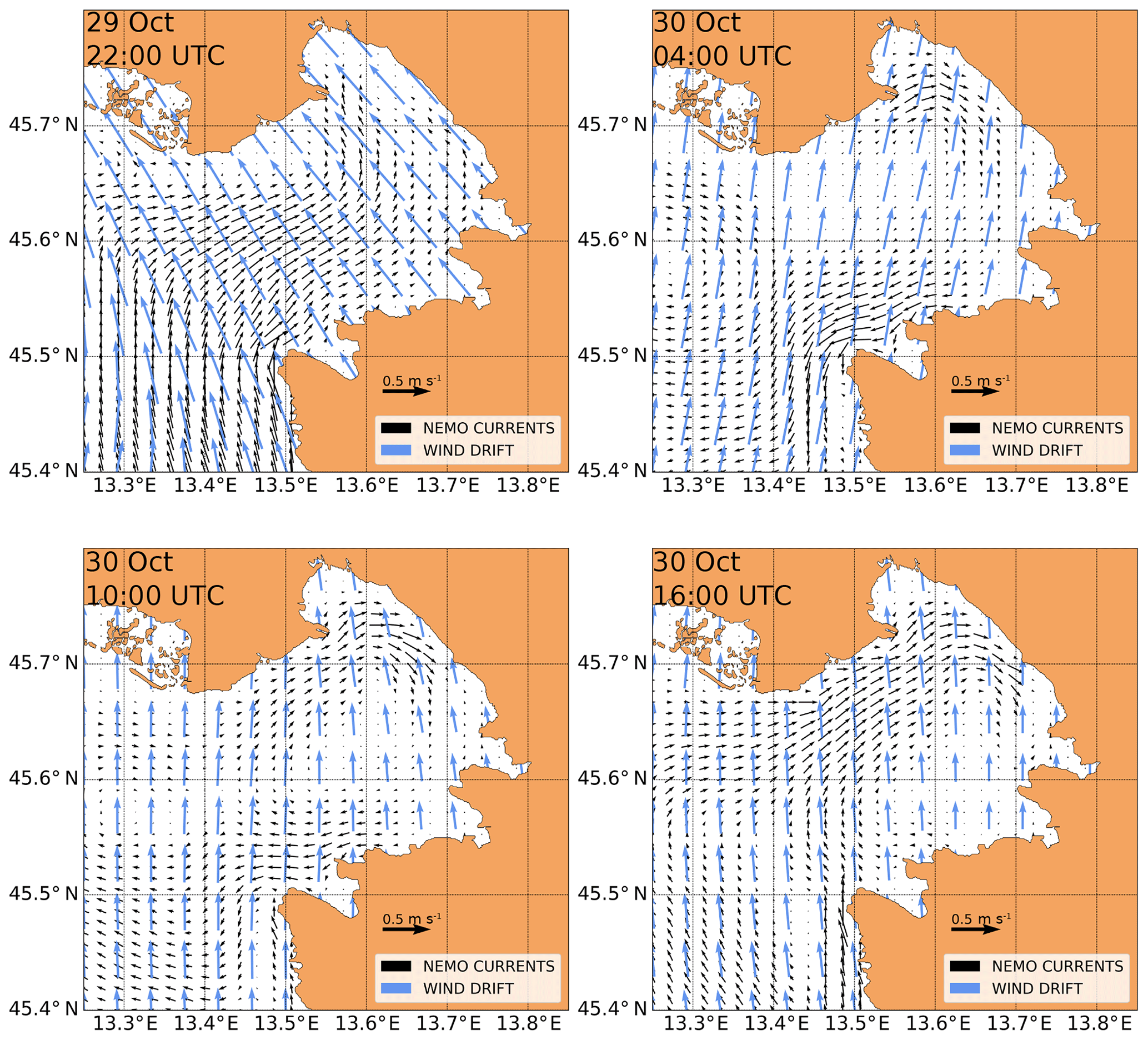
Figure 7 The 6-hourly same-scale snapshots of NEMO currents (black arrows) and ALADIN SI 10 m wind u₁₀ induced wind drift (blue arrows) over the period of the windsurfer's drift. Only purely downwind arrows with no crosswind departure from the ALADIN SI wind velocity direction are plotted, computed as a_∥u₁₀ using OpenDrift person-in-water downwind slope $a_{\parallel }=\mathrm{1.93}\mathit{\%}$. Only every third wind point is plotted for clarity. Arrow lengths from both fields are commonly scaled and both arrow length units are metres per second.

Figure 7 depicts current and wind drift inputs to both models over the period of the windsurfer's drift. The wind drift seems to be the dominant driving factor of the windsurfer's drift, its speed being roughly double that of the surface currents. Wind drift prior to (not shown) and at 22:00 UTC has a clear southeasterly direction (at Umag – offshore) at roughly 140–160^∘, consistent with the windsurfer's experience and his inability to reach Savudrija in time. During the night the wind direction shifts to south-southwesterly to about 190^∘, also consistent with his experience. In the morning of 30 October 2018 and through the day, the wind direction is predominantly southern at 180^∘. This is all in agreement with the direction shift measured at the Vida buoy (Fig. 5).

NEMO currents at 22:00 UTC indicate a northward direction along the coast of Istria and also a surface inflow along all but the northernmost part of the opening of the Gulf of Trieste. The northernmost part along the northern coast of the gulf most likely shows no notable inflow due to inertial westward coastal current from the Soča River, which manifests itself as an outflow from the gulf, confined to this part of the coast (see Fig. 1 for the related river plume).

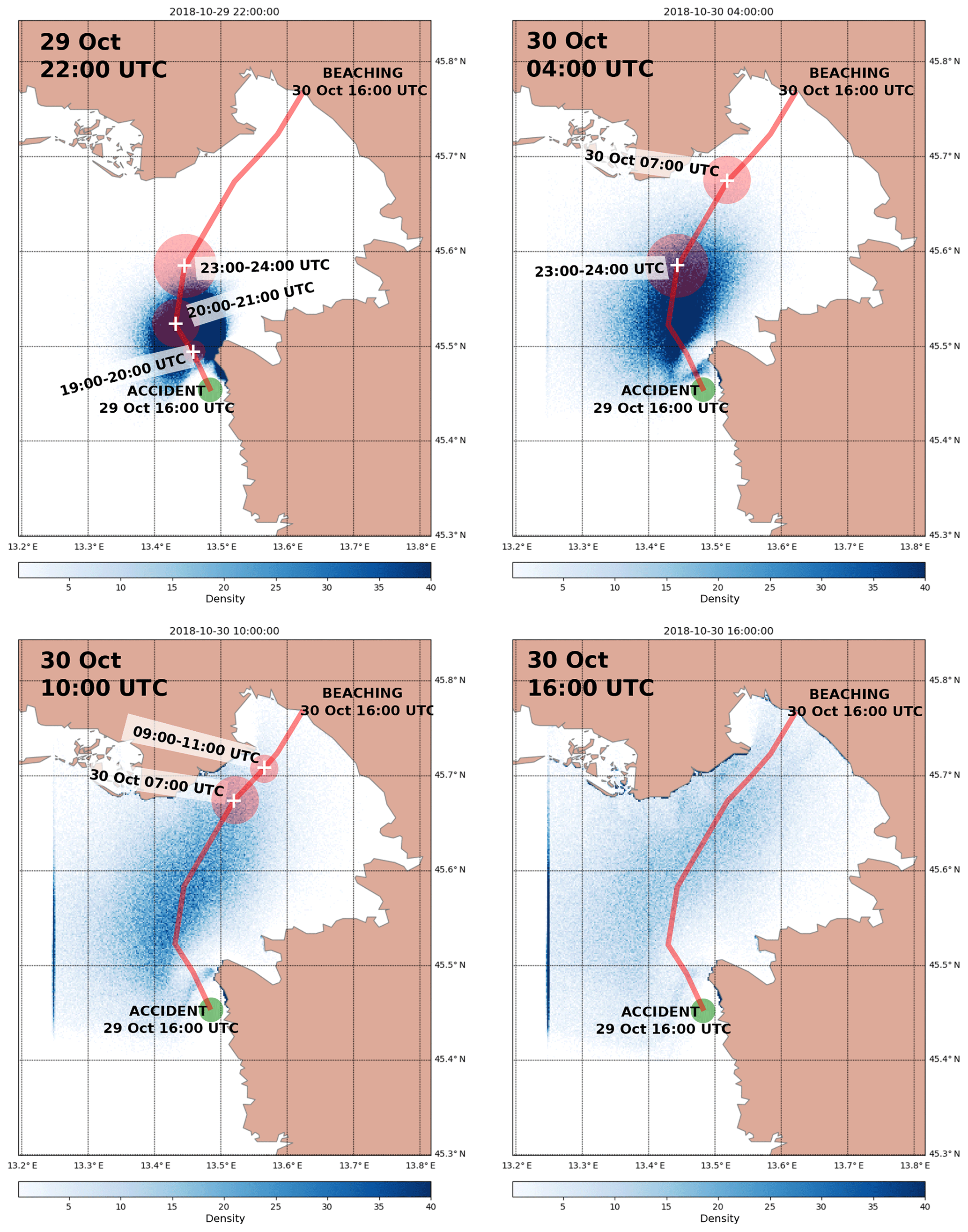
Figure 8 Lagrangian particle density (number of particles per cell area) from the OpenDrift simulation of the person-in-water object type. Lagrangian simulation drift is depicted every 6 h (indicated by a timestamp in the upper left corner of each panel) after the accident on 29 October 2018 16:00 UTC. The red line denotes drift trajectory as reconstructed by the survivor. White crosses and time inserts denote locations and times from the survivor's trajectory estimate, while red circles around crosses denote the survivor's uncertainty estimates of the respective location.

4.3 Lagrangian simulation results

In this section we present OpenDrift simulations with NEMO model current inputs and ALADIN SI 10 m wind inputs during 29 October 2018 16:00 UTC and 30 October 2018 16:00 UTC. Simulations were performed running forward-propagation in time, starting particle drift from the accident location at October 2018 16:00 UTC.

OpenDrift results for the drifting-object type “person in water” are presented in Fig. 8, which shows 6-hourly snapshots of particle densities (number of particles per cell area), initially seeded in the green region at 29 October 2018 16:00 UTC. To ensure smooth maps of particle density, a large number (50 000) of virtual particles of the type person in water were released at the accident location at the accident time and advected forward in time in 12 min time steps (0.2 h) for 24 h. Cells over which the particles are counted were again chosen to be of 150 m×150 m dimensions. This reduction in cell computation area was again done because the original NEMO grid resolution (1000 m×1000 m) is too coarse to produce smooth maps of particle density. After 6 h, at 22:00 UTC, the set of the particles envelops the estimated windsurfer location, but the centre of gravity of the particle set is lagging southeast of the survivor's estimated location.

A shift in the wind direction from southeast to south-southwest (see Fig. 5), occurring sometime after 29 October 22:00 UTC and lasting until 04:00 UTC, causes a corresponding shift in particles' drifting directions and a stretched dispersal of the particle set along the survivor's trajectory estimate.

The first particles beach on the northern shore of the gulf between 04:00 and 10:00 UTC. This predominantly occurs between Grado and the Soča River mouth. Particles in the gulf propagate along the reconstructed trajectory, but with increasing lateral and axial extent. At 10:00 UTC the set is dispersed over the northwestern half of the Gulf of Trieste and are stretched roughly along the survivor's trajectory. While the majority of particles lag behind the survivor's estimated location, the set does extend over the survivor's estimated location, which is enveloped by the forefront of the particle set.

After 24 h the particle set is almost homogeneously dispersed over the northwestern half of the gulf, with some of the particles beaching within 2 km of the actual beaching location.

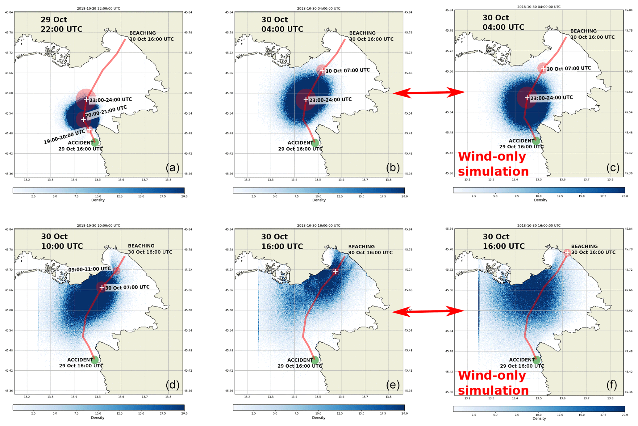
Figure 9 Same as Fig. 8 but for the person-with-a-surfboard object type. Panels (c, f) depict simulation results with wind-only input (and ocean currents set to zero) after 12 and 24 h of drift.

OpenDrift results for the drifting-object type person with a surfboard are presented in Fig. 9. After 6 h, at 22:00 UTC, the set of the particles envelops the estimated windsurfer location, and the centre of gravity of the particle set is closer to the survivor's estimated location than in the person-in-water case. This particle set also overlaps with the higher-density region of the northwestern pathway from HF radar current back-propagation simulation results at 29 October 2018 22:00 UTC presented in Fig. 4d.

A shift in the wind direction from southeast to south-southwest (see Fig. 5), occurring sometime after 29 October 22:00 UTC and lasting until 04:00 UTC, again causes a corresponding shift in particles' drifting directions, but the dispersal of the particle set along the survivor's trajectory estimate is somewhat lesser than in the person-in-water case. At 04:00 UTC the majority of the particles are lagging behind (i.e. mostly located southwest of) both the survivor's location estimate and the densest region from the northwestern branch of the back-propagation simulation (Fig. 4d). This is consistent with the fact that NEMO-modelled currents underestimate HF radar measurements used for back-propagation simulations.

At 10:00 UTC the particle set is dispersed between Grado and the Soča River mouth, again lagging behind the both survivor's location estimate and the northwestern branch of the back-propagation simulation (Fig. 4b). When compared to the person-in-water scenario, this particle set is however more clearly localized along the northern shore of the gulf.

After 24 h the particle set is densest around the Soča River mouth, but with a clearly visible streak of particles beaching within 2 km of the actual beaching location. This higher localization represents some improvement over the entire northwestern half of the Gulf of Trieste, indicated by the person-in-water simulation. In any case a quantitative comparison is performed below to further elucidate performances of both drift simulations.

Figure 9 contains also a third separate column which depicts results of a wind-only simulation (with ocean currents artificially set to zero) after 12 and 24 h of drift, i.e. at 30 October 04:00 and 16:00 UTC respectively. Comparison with the first two columns (depicting full simulations with both winds and currents) demonstrates ocean current influence on particle dispersal. Under rather homogeneous wind conditions (see Fig. 7), particle dispersal due to wind is highly isotropic throughout the simulation period. Being highly inhomogeneous itself, the ocean current pattern in the gulf adds asymmetry to the wind dispersal pattern. This effect somewhat elongates the slick of particles and advects them further along the Italian coast closer towards Sistiana.

Given available data (or lack thereof) a quantitative comparison between the drift simulations can only be based on the beaching point, which is known. To pursue this we calculated the distribution of stranded and active (non-stranded, still in the water column) particles and plotted their histogram over distances from the beaching location at beaching time and also 6, 12, 18, and 24 h after the beaching time. Distributions at beaching time and particle accumulation after the beaching time are depicted in Fig. 10.

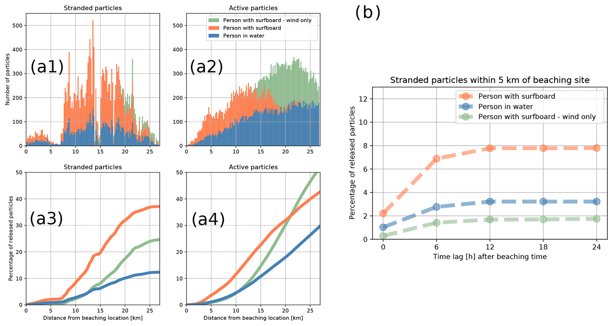
Figure 10 (a1, a2) Stranded (a1) and active (a2) particle distribution over distances from the beaching location at beaching time. Panel (a3, a4): cumulative particle distributions of stranded (active) particle distribution, shown in (a1, a2), over distances from the beaching location at beaching time. (b) Time dependence of accumulated percentage of particles within 5 km of the beaching site.

Panel A2 in Fig. 10 indicates that at beaching time the distribution maximum of active person-with-a-surfboard particles is positioned about 12 km from the beaching site. It is also positioned 15 km closer to the beaching point than the distribution maximum of person-in-water particles. This indicates (a) better performance of person-with-a-surfboard particles and (b) a time lag in the movement of all types of particles. As mentioned above, this is very likely due to the NEMO model surface current underestimation during the event – this claim is further backed by the fact that WERA HF back-propagation simulations in Sect. 4.1 seem temporally consistent with the survivor's estimate (Fig. 4) and show little lag after 18 h of drift.

These conclusions are also implied by the particle distributions in Figs. 8 and 9: at beaching time, person-in-water particles are dispersed over a much wider area than those of person-with-a-surfboard type. Figure 10a2 reflects that.

However, and regardless of this lag, when focusing on the accumulation of stranded particles (Fig. 10a3, b), we see that at beaching time about twice as many person-with-a-surfboard particles stranded within 5 km of the beaching point than those of the person-in-water type. The same holds for particles stranding within a 10 km radius. Within a 20 km radius this ratio triples. These results quantitatively substantiate claims of better performance of the person-with-a-surfboard particle type for this case study.

Figure 10b shows the percentage of stranded particles within a 5 km distance of the beaching site in the hours after the beaching. This percentage saturates on the scale of 6 h, giving us an estimate for the time lag between the actual survivor beaching and beaching of the majority of simulation particles.

We conclude this section with a brief comment on wind-only simulations with person-with-a-surfboard type. These simulations under homogeneous wind conditions exhibit highly isotropic spatial dispersion of particles, unlike the two scenarios which take into account ocean currents. This leads to slower accumulation of particles within a 5 km radius of the beaching point (Fig. 10a3, b). At these distances and by this metric, wind-only simulations are the worst performer of all three. Without putting too much weight on wind-only simulation – this does indicate the importance of topographically constrained ocean currents in semi-enclosed basins like the Gulf of Trieste even in seemingly wind-dominated situations.

5 Conclusions

In the paper we present a modelling analysis of the 24 h marine drift by the windsurfer whose mast broke on 29 October 2018 16:00 UTC, during a 29 October 2018 scirocco storm in the northern Adriatic. We conduct an interview with the survivor in order to reconstruct his trajectory and its uncertainty. The survivor knows the coast of the Gulf of Trieste very well but had no GPS or watch on him during the drift. His reconstruction of the drift trajectory is therefore burdened with error. To estimate this error we used HF radar surface current measurements, which cover the second half of his drift, and we employed them for upwind and upstream temporal back-propagation simulations starting at the beaching site at beaching time, both of which are exactly known. These back-propagation simulations were found to be largely consistent with the survivor's reconstruction, offering some confidence that while not perfect the reconstructed trajectory can nevertheless serve as a qualitative guide for Lagrangian tracking.

We then present ocean circulation (NEMO), atmosphere (ALADIN SI), and OpenDrift Lagrangian tracking models, used to perform forward-propagation simulations of this trajectory, starting from the accident location. We present available marine measurements (regional coastal buoy Vida and HF surface current radar) to qualitatively assess marine conditions in the Gulf of Trieste during the period of the drift.

The OpenDrift Lagrangian tracking model was employed using two types of marine drift parameterizations: person in water and person with a surfboard. Stokes drift from a wave model was not explicitly included in OpenDrift forcing data since these effects are already implicitly present in the downwind and crosswind drift parameterizations, deduced from observations (Breivik and Allen, 2008).

To quantify performance of both drift parametrization types, we calculated distributions of particle distances from the beaching location for both object types. Simulations using the object type person with a surfboard yield the best performance, with the highest number of particles stranded within 5 km of the beaching location. Distribution maximum of the person-with-a-surfboard particle type is positioned about 15 km closer to the beaching point than the distribution maximum of the person-in-water particle type. Both scenarios however lag behind the estimated drift which most likely results from NEMO model underestimation of surface currents during the event. For both drift parametrization types of accumulation of particles, stranded within 5 km of the beaching location, saturates roughly 6 h after the actual beaching time.

A control run of wind-only forcing was also simulated, and this setup was the worst performer of all three, indicating the importance of topographically constrained ocean currents in semi-enclosed basins like the Gulf of Trieste even in wind-dominated situations.

Results in this paper indicate that any rescue response in the 29 October 2018 case would certainly benefit from OpenDrift simulations using the person-with-a-surfboard object type. However, while one can clearly benefit from using the most appropriate drift parametrization, lack of information during an actual event often complicates the decision of which parametrization to use.

It is also worth mentioning that given the location of the accident, a drift under bora wind conditions seems substantially more dangerous. Bora wind is typically much colder and can, regardless of its short fetch, generate comparable marine conditions in the northern Adriatic, but its nautical direction is 60^∘, i.e. completely offshore in northern Istria. Marine drift initiated in Umag (or, more likely, at a popular bora windsurfing spot near the Cape of Savudrija) during the bora wind would have lasted days, and possibly more than a week if the person would get advected westward far enough to join Western Adriatic Current flowing southward along the Italian coast. Reliable and operational circulation models, coupled to calibrated Lagrangian tools like OpenDrift, would be an invaluable decision support for any rapid rescue attempt.