the Creative Commons Attribution 4.0 License.
the Creative Commons Attribution 4.0 License.
 | 20 Jan 2020
Modeling the effects of sediment concentration on the propagation of flash floods in an Andean watershed
María Teresa Contreras
Cristián Escauriaza
Rain-induced flash floods are common events in regions near mountain ranges. In peri-urban areas near the Andes the combined effects of the changing climate and El Niño–Southern Oscillation (ENSO) have resulted in an alarming proximity of populated areas to flood-prone streams, increasing the risk for cities and infrastructure. Simulations of rapid floods in these watersheds are particularly challenging, due to the complex morphology, the insufficient hydrometeorological data, and the uncertainty posed by the variability of sediment concentration. High concentrations produced by hillslope erosion and rilling by the overland flow in areas with steep slopes and low vegetational covering can significantly change the dynamics of the flow as the flood propagates in the channel. In this investigation, we develop a two-dimensional finite-volume numerical model of the nonlinear shallow water equations coupled with the mass conservation of sediment to study the effects of different densities, which include a modified version of the quadratic stress model to quantify the changes in the flow rheology. We carry out simulations to evaluate the effects of the sediment concentration on the floods in the Quebrada de Ramón watershed, a peri-urban Andean basin in central Chile. We simulate a confluence and a total length of the channel of 10.4 km, with the same water hydrographs and different combinations of sediment concentrations in the tributaries. Our results show that the sediment concentration has strong impacts on flow velocities and water depths. Compared to clear-water flow, the wave-front velocity slows down more than 70 % for floods with a volumetric concentration of 60 % and the total flooded area is 36 % larger when the sediment concentration is equal to 20 %. The maximum flow momentum at cross sections in the urban area increases 14.5 % on average when the mean concentration along the main channel changes from 30 % to 44 %. Simulations also show that other variables such as the arrival time of the peak flow and the shape of the hydrograph at different locations along the channel are not significantly affected by the sediment concentration and depend mostly on the steep channel morphology. Through this work we provide a framework for future studies aimed at improving hazard assessment, urban planning, and early warning systems in urban areas near mountain streams with limited data and affected by rapid flood events.
- Article
(10854 KB) - Full-text XML
- Companion paper
- BibTeX
- EndNote


Flash floods with high sediment concentrations are common natural events in mountain rivers, which generate hazards in cities and other smaller human communities located near river channels (EEA, 2005; Wilby et al., 2008). In spite of the continued efforts to provide structural and nonstructural measures to control flood hazards in general, economical losses have increased in recent decades (Slater et al., 2015), and flood risks and vulnerability associated with various economic, political, and social processes are also expected to increase in the future (Pelling, 2003; Blaikie et al., 2004; Bankoff et al., 2004).
The spatial and temporal distribution of precipitation, the morphology of the basin, soil properties, and vegetation characteristics naturally influence the magnitude and frequency of floods and sediment transport. Anthropogenic factors also affect the volume and peak discharges of floods in mountain rivers. Climate models predict a larger frequency of intense precipitation events and cyclonic weather systems that will increase the vulnerability in many mountainous regions in the future (Sanders, 2007; Arnell and Gosling, 2014; Boers et al., 2014). An amplification of the flood hazards is also expected due to the continuing expansion of cities located in floodplains (Jongman et al., 2012; Hirabayashi et al., 2013), accelerated urbanization processes (Schubert et al., 2008), lack of urban planning (Rugiero and Wyndham, 2013), and changes in land use and cover (Kundzewicz et al., 2014).
The effectiveness of assessing flood hazards and designing strategies aimed at reducing potential damage caused by flooding is closely related to understanding the dynamics of the flow in real conditions. Recent physical models and experiments have provided relevant insights into the flow physics of flash floods in extreme conditions (e.g., Testa et al., 2007). Field-based and experimental research over complex topography, however, requires large facilities with advanced instrumentation to provide high-resolution measurements that are also limited by the spatiotemporal scales at which rapid floods occur. Numerical models, on the other hand, have also become fundamental tools to advance our understanding of the dynamics of floods, evaluating complex scenarios, and predicting water depths and flow velocities in arbitrary geometries (Siviglia and Crosato, 2016). Simulations yield detailed information on the flood dynamics, which are sometimes experimentally inaccessible or cannot be directly measured in the field. They can also complement measurements, becoming effective tools for urban planning and for designing early warning systems during flood events (Mignot et al., 2005; Schubert and Sanders, 2012).
In most hydrodynamic models to simulate flood propagation, the nonlinear shallow water equations (NSWEs) or Saint-Venant equations are employed to describe the dynamics of the flow in homogeneous and incompressible fluids. They are obtained by vertically averaging the three-dimensional Navier–Stokes equations, assuming a hydrostatic pressure distribution, resulting in a set of horizontal two-dimensional (2-D) hyperbolic conservation laws that describe the evolution of the water depth and depth-averaged velocities in space and time. In flows where discontinuities and rapid wet–dry interfaces develop, numerical models employ Godunov-type formulations, solving a Riemann problem at the interfaces of the elements of the discretization (Anastasiou and Chan, 1997; Toro, 2001).
The development of efficient and accurate numerical models to simulate flash floods, however, is far from trivial, since multiple factors control the dynamics of the flow. This is particularly true in mountainous regions, where rivers are characterized by three important features that complicate their representation: (1) complex bathymetries and steep slopes produce rapid changes on velocities and water depths, formation of bores, and wet–dry interfaces; (2) large sediment concentrations directly affect the flow hydrodynamics by introducing additional stresses that alter the momentum balance of the instantaneous flow; and (3) there is a lack of accurate field data, used for validation, due to the difficulties on measuring hydrometeorological variables in high-altitude environments, with difficult access, and during episodes of severe weather.
The Andes mountains in South America incorporate all these characteristics, and they have been the site of many recent catastrophic events, leaving a significant human toll and economic losses (Wilcox et al., 2016). The region is characterized by rapid floods with high concentrations of sediment, generally produced by hillslope erosion and rilling by the overland flow in areas with steep slopes and low vegetational covering. Additional factors, such as the storms caused by the South American monsoon (Zhou and Lau, 1998) and El Niño–Southern Oscillation (ENSO), can generate anomalously heavy rainfall (Holton et al., 1989; Díaz and Markgraf, 1992), producing a great volume of liquid precipitation and significant erosion and sediment transport in the flow.
High sediment concentrations during floods cause additional stresses produced by the increase in the density and viscosity of the water–sediment mixture. Models need to account for the internal stresses that emerge from the particle–flow and particle–particle interactions in the sediment-laden flow. These stresses transform the rheological behavior of the mixture, represented by additional terms of momentum transfer in the governing equations. A wide variety of rheological models have been proposed depending on the sediment properties and concentration (see for instance Bingham, 1922; Bagnold, 1954; O'Brien and Julien, 1985, among others). These approaches are based on empirical equations that have been estimated from laboratory studies (Parsons et al., 2001) or back-calibrated from past events (Naef et al., 2006).
The main objective of this investigation is to gain fundamental insights into the effects of high sediment concentrations on the propagation of floods in an Andean watershed. We develop a 2-D finite-volume numerical model of the NSWEs, building on the work of Guerra et al. (2014), which incorporates the effects of the sediment load on the dynamics of the flow over natural terrains and complex geometries. First we validate the sediment-coupling module by using three benchmark cases including an analytical solution, numerical simulations, and experiments. Then we carry out simulations of flows with different sediment concentrations in the two main tributaries of the Quebrada de Ramón watershed, located at the foothills of the Andes mountain range, to the east of Santiago, Chile, where part of the city occupies the lower section of the river basin. From the simulations we evaluate the effects of the sediment load on the evolution of the flow depth and velocity, and we link the hydrodynamic response of the river channel to the variations in sediment concentration. The analysis provides quantitative information of the hyperconcentrated flood propagation, including the changes in the total flooded area and momentum at cross sections of the flow, among other parameters for flood hazard assessment.
The paper is organized as follows. The governing equations of the model and its implementation in the study area are presented in Sects. 2 and 3, respectively. In Sect. 4, we study the consequences of high concentrations on the dynamics of the flow, the total momentum in cross sections of the river, and local water depths and velocities. In Sect. 5, we discuss the results in the context of the interactions between geomorphic controls of the flood propagation and the sediment concentration of the flow. Finally, in Sect. 6 we summarize the findings of this investigation.
2.1 Governing equations
Rapid floods over the complex topography of mountainous regions are commonly affected by high sediment concentrations, which change the rheology of the flow. By assuming that the mixture preserves the Newtonian constitutive relation between stress and rate of strain, the NSWEs can be modified to account for the heterogeneous density distribution in space and time (Loose et al., 2005; Michoski et al., 2013).
The NSWE model implemented in this investigation has the following assumptions: (i) hydrostatic pressure distribution, (ii) negligible vertical velocities, (iii) vertically averaged horizontal velocities, (iv) horizontal heterogeneous fluid density, (v) homogeneous density in the vertical direction, and (vi) a fixed bed (neither erosion nor deposition). The momentum sources and sinks consider the gravity term, the bed resistance, and the rheology of the mixture, including the yield stress, Mohr–Coulomb stress, viscous stresses, and turbulent and dispersive stresses, as discussed in Sect. 2.2.
If we denote the dimensional variables of the flow with a hat (), the NSWEs coupled with the sediment concentration are written as follows:
where is the flow depth, and and are the depth-averaged velocities in the Cartesian coordinate directions and , respectively. The bed elevation is denoted as , g is the acceleration of gravity, represents the time, is the density of the water–sediment mixture, C is the volumetric concentration of sediment, and and are the total stresses.
Here we follow the same procedure outlined in Guerra et al. (2014), expressing the governing equations in nondimensional form using a characteristic velocity scale 𝒰, a scale for the water depth ℋ, and a horizontal length scale of the flow ℒ. In this case, two nondimensional parameters appear in the equations, i.e., the relative density between the sediment and water and the Froude number .
To adapt the computational domain to the complex arbitrary topography in mountainous watersheds, we use a boundary fitted curvilinear coordinate system, denoted by the coordinates (ξ,η). Through this transformation we can have a better resolution in zones of interest and an accurate representation of the boundaries. We perform a partial transformation of the equations, and we write the set of dimensionless equations in vector form as follows:
where Q is the vector that contains the nondimensional Cartesian components of the conservative variables h, hu, hv, and hC, which are obtained by replacing the density of the mixture , where ρw is the water density and ρs the sediment density.
The Jacobian of the coordinate transformation J is expressed in terms of the metrics ξx, ξy, ηx, and ηy, such that (Lackey and Sotiropoulos, 2005; Guerra et al., 2014). The fluxes F and G in each coordinate direction are expressed as follows:
where U1 and U2 represent the contravariant velocity components defined as and , respectively.
The model considers three source terms: SB contains the bed slope terms, SS corresponds to the bed and internal stresses of the flow, and SC incorporates the effects of the spatial gradients of sediment concentration. This last term might be important in rapid flows with large concentration gradients, such as dam breaks with sediment-laden debris flows (Cao et al., 2004), and in cases with interactions of clear-water and hyperconcentrated flows. The source vectors are expressed as follows,
Since the objective of this investigation is to exclusively study the impacts of sediment transport on the hydrodynamics of rapid floods in mountain rivers, where the geomorphic features of the channel play a significant role in flood propagation, we are not considering the erosion or deposition of the bed. The channel of the Quebrada de Ramón stream has a long bedrock section, and the urban area is completely paved. No significant erosion of the channel was reported in the most recent flood, but these conditions cannot apply to other similar cases (e.g., Wilcox et al., 2016).
It is important to note that mountain rivers with steep slopes in peri-urban watersheds exhibit a wide variety of bed conditions, i.e., bedrock channels, boulders, coarse gravel surfaces, armoring, sand and gravel mixtures, and the concrete surface of the urban setting. The complexity of these environments and the unknown effects of the high sediment concentrations that originate in the high-altitude sections of the mountains prompted the development of this model that couples the transport equation to the flow in mass and momentum with high resolution. The system of governing Eq. (5) is solved using a well-balanced 2nd-order finite-volume method with an efficient Riemann solver that incorporates hydrostatic reconstruction and a semi-implicit fractional-step time integration approach (Guerra et al., 2014) (see Appendix A). Here we incorporate the density and rheological models that are described in the following section.
2.2 Rheological model
The classification and rheology of gravity-driven flows with higher concentrations usually depend on the particle size distribution and sediment composition. Depending on these characteristics, the flows can vary from nearly dry landslides to water flow, with intermediate conditions such as debris flows, mudflows, and mud floods (Julien and León, 2000; Naef et al., 2006). The rheological behavior that determines the magnitude of the momentum losses is incorporated in additional source terms of the hydrodynamic model previously presented in vector SS in Eq. (7). As summarized by Ancey (2007), gravity-driven flows can be described by different rheological models such as those of Bagnold, Bingham, Voellmy, or Coulomb, depending on the assumptions of the effects of the particles on the dynamics of the flow. In our numerical model we implement the quadratic shear stress model developed by O'Brien and Julien (1985) (see also O'Brien et al., 1993), which represents the total stress in each coordinate direction i, as follows:
where represents the sum of the Mohr–Coulomb and yield stresses, the second term is the viscous shear stress that depends on the dynamic viscosity of the mixture and the vertical velocity gradient expressed as a function of the Cartesian velocity components ui. The last term corresponds to the sum of the turbulent and dispersive stresses, which depend quadratically on the velocity gradient and the inertial shear stress coefficient , defined by the following equation:
where is the Prandtl mixing length (Julien and León, 2000), cBd is an empirical proportionality constant equal to 0.01 according to Bagnold (1954), ds is the median sediment diameter, and λ is Bagnold's linear concentration, which corresponds to the ratio between the grain diameter and the mean free dispersion distance. The magnitude of λ is related to the volumetric concentration of the mixture and the maximum volumetric static concentration C∗, as defined by Bagnold (1954).
In the present numerical model we modify the quadratic model of O'Brien and Julien (1985) to represent the stresses for a wide range of sediment concentrations, clearly expressing the contribution of each physical mechanism as the combination of relations that account for the stresses, which have been obtained from experiments or physically based formulas. To determine the values of the source terms defined as in Eq. (7), the stresses are nondimensionalized, depth-integrated, and added in the source term vector for each coordinate direction, such that the total stresses are expressed as
where Syield represents the sum of the yield and Mohr–Coulomb stress, the viscous stress, and the sum of the dispersive and turbulent stresses. Each of these terms is computed separately from empirical formulas.
The yield and Mohr–Coulomb stresses Syield are jointly calculated from the following expression:
in which the yield shear stress and the density of the mixture are nondimensionalized with the scale of the inertia ρw𝒰2 and the water density ρw. The yield stress is isotropic and calculated using the following empirical relation given in SI units:
where for typical soils, the experimental coefficients a and b are equal to 0.005 and 7.5, respectively (Julien, 2010).
The viscous term is computed from the bed stress in each direction and , using the laminar friction coefficient defined as , where k is the viscous resistance parameter equal to 64 in open-channel flows (Sturm, 2001). The Reynolds number is defined as , where the dynamic viscosity of the mixture is nondimensionalized as . Thus, the expression used to represent the viscous losses is written as follows:
To estimate μm we use the formula proposed by Eyring (1964) and Thomas (1965). This relation is a function of the volumetric sediment concentration in the mixture and the dynamic viscosity of water μw in SI units:
To compute the last term in Eq. (11), Std, a Manning or Chézy coefficient is used to represent the friction factor Cf in the bed stress formula, resulting in the following expression for each Cartesian coordinate direction:
Since Std represents the sum of friction, turbulence and dispersive stresses, we use either a modified Manning ntd or Chézy Cztd coefficients. To estimate their value we add two Darcy–Weisbach friction factors, denoted as ft and fd, representing the turbulent and dispersive effects, respectively. To compute ft, we use Colebrook's equation:
The value of ft is calculated as a function of the depth of the mixture h, the Reynolds number, and the bed-specific roughness , which is estimated as follows (Bathurst, 1978):
To account for the dispersive effects, fd is calculated using the relation proposed by Takahashi (2007):
where ρs and ρw are the sediment and water densities, respectively, and λ is Bagnold's linear concentration defined previously in Eq. (10). In general, numerical simulations show that the turbulent friction coefficient ft is significantly smaller than the dispersive factor fd (D'Aniello et al., 2015). Dispersive effects, however, become important for low values of relative roughness (), as discussed in detail by Julien and Paris (2010).
To obtain the terms , we use the following relation proposed by Julien (2010) to transform the combined Darcy–Weisbach friction coefficient into an equivalent Manning–Chézy coefficient:
Appendix B contains tests of this model comparing to analytical solutions, numerical simulations, and experiments to verify its precision and evaluate the flexibility of the model to address the flood propagation in Andean environments.
As has been previously mentioned, one of the cases where the sediment concentration plays a significant role is in the flood propagation in mountain rivers. We select as a study case the Quebrada de Ramón watershed in the Andes of central Chile to evaluate how the hydrodynamics of the flow are altered by the magnitude of the sediment concentrations. We simulate the same scenario, but we modify the volume sediment concentration in a range of 0 %–60 %. We locally characterize the depths and velocities of the flow as the flood propagates, but we also evaluate the extension of flooded area and the momentum of the flow in the lower section of the watershed, within the city of Santiago.

Figure 1Satellite image of the Quebrada de Ramón watershed and the computational domain. The area enclosed by the black line is defined from the lidar topography and incorporates the section of the city around the river channel. The main channel is depicted in blue and the tributary in turquoise. Background image of the terrain from © Google Earth.
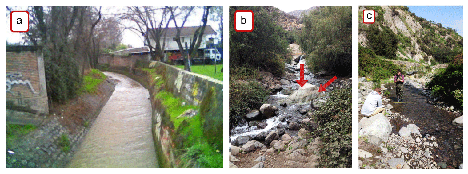
Figure 2Three photos along the Quebrada de Ramón stream from downstream to upstream: (a) the channelized section, (b) the floodplain, and (c) the confluence of the Quebrada de Ramón and the Quillayes streams.
In this watershed there are two major tributaries draining the north and south sections of the watershed. We define the computational domain shown in Fig. 1, which comprises a total distance of 10.4 km along the main channel. The highest part of the computational domain is located at an elevation of 2212 m a.s.l., with the Quebrada de Ramón stream (QR) and the Quillayes stream (Qui) approaching from the north and south, respectively. The upstream boundary of the domain is located 3 km upstream of the confluence (Fig. 2c). The channel downstream from the confluence continues to the flood zone, with a single main river channel shown in Fig. 2b, and it ends at an elevation of 652 m a.s.l., where the stream has been channelized in the city, as shown in Fig. 2a. A curvilinear boundary-fitted grid is used to perform the simulations, consisting of a total of 10 070×218 grid nodes. The grid resolution varies progressively in the flow direction from 0.5 m upstream and near the confluence to 2 m resolution within the flooding zone. In the cross-stream direction, the mean resolution of the grid close to the channels is approximately 1 m. To construct the grid, we use a 1 m resolution lidar of the area around the channels. The lidar data are coupled to a 30 m resolution digital elevation model (DEM) from satellite images for the rest of the watershed.
The bed roughness is represented by a mean sediment grain diameter ds. Field measurements are used to interpolate the values of ds in the entire computational domain using the nearest-neighbor method. The mean sediment grain size distribution is shown in Fig. 3, along with the seven points where we report the dynamics of the flow, which include locations at the highest elevation of the domain (denoted as QR-U and Qui-U), upstream of the confluence (QR-D and Qui-D), downstream of the confluence (QR-C), in the flooding zone (QR-F), and at the outlet (QR-E).
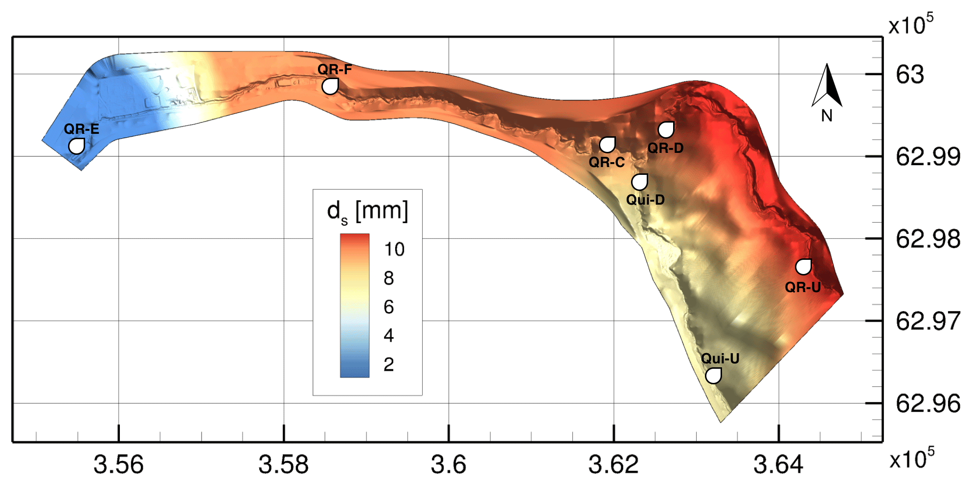
Figure 3Distribution of the mean sediment size in millimeters. White circles denote the measurement sites where we report the propagation of the flood.
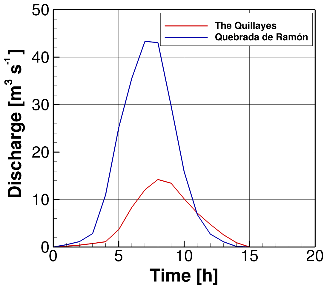
The hydrographs of the event studied in this investigation for the two main rivers that correspond to the tributaries of the confluence are shown in Fig. 4. The return period of these hydrographs has been estimated as 50 years, and this was obtained from a continuous semi-distributed hydrological model built at the HEC-HMS, for the 1971–2010 period (Ríos, 2016). This case is selected since the peak flow at the outlet is expected to significantly exceed the capacity of the channelized section in the city.
The actual sediment concentration during flash floods in Andean watersheds is unknown in most cases. In addition to the lack of information in these rivers, landslides due to erosion produced by soil saturation in the steep slopes of the mountains are common. These conditions can considerably increase the sediment supply to the streams during flood events, with material that does not come from the channel but mostly from hillslope erosion. We study the dynamics of the flood for different scenarios by carrying out a series of simulations to compare and understand the flood hazards and effects of hyperconcentration on the two main streams of the Quebrada de Ramón watershed.
We simulate four different scenarios considering different concentrations of 0 %, 20 %, 40 %, and 60 % equal in both streams. Two other cases are simulated, with concentrations of 20 % in the Quebrada de Ramón stream and 60 % in the Quillayes stream and vice versa.
The river bed is considered dry at the beginning of the simulation, to avoid the additional effects of different sediment concentrations of the initial flow.
We perform the simulations for a total physical time of 1 d, using a simulation time step defined by the Courant–Fiedrichs–Lewy (CFL) stability criterion, defined as
which in this case is set equal to CFL=0.9.
The inflow boundary condition in Fig. 4 is used at the eastward boundary, and open boundary conditions are considered at all the other boundaries of the computational domain.
To evaluate the impacts of different sediment concentrations on the flood dynamics, in the following subsections we analyze the flow hydrodynamics including (1) the position and velocity of the flood wave front, (2) the peak flow and arrival time, (3) the flooded areas, (4) the effect of the sediment concentration on the depth and flow velocity, and (5) the momentum of the flow in the urban zone.
4.1 Position and mean velocity of the wave front
To quantify the propagation of the flood along the channels and the arrival time of the flood to the city, we compute the mean velocity of the wave front by tracking its position in time. Table 1 shows the mean velocity in the section upstream of the confluence, for the Quebrada de Ramón and Quillayes streams. As can be anticipated, the velocity of the wave front decreases with the concentration, as interparticle collisions and internal stresses reduce the momentum of the flow, increasing flow resistance. Note that the flood propagation velocity is very sensitive to variations in concentration in more dilute conditions. Overall, the velocity for a concentration of 20 % is 30 % slower than clear-water flow in both streams. On the other hand, when the concentration increases from 40 % to 60 %, the velocity is reduced by less than 10 %. The mean wave front propagation velocity seems to be decreasing quadratically with the concentration in this case (R2=0.983 and R2=0.9868 for each stream).
Table 1Mean velocity of the front for different sediment concentrations. In parentheses, the percentage change from clear water is shown.
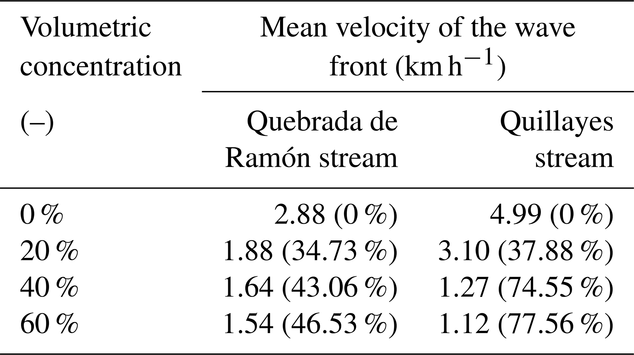
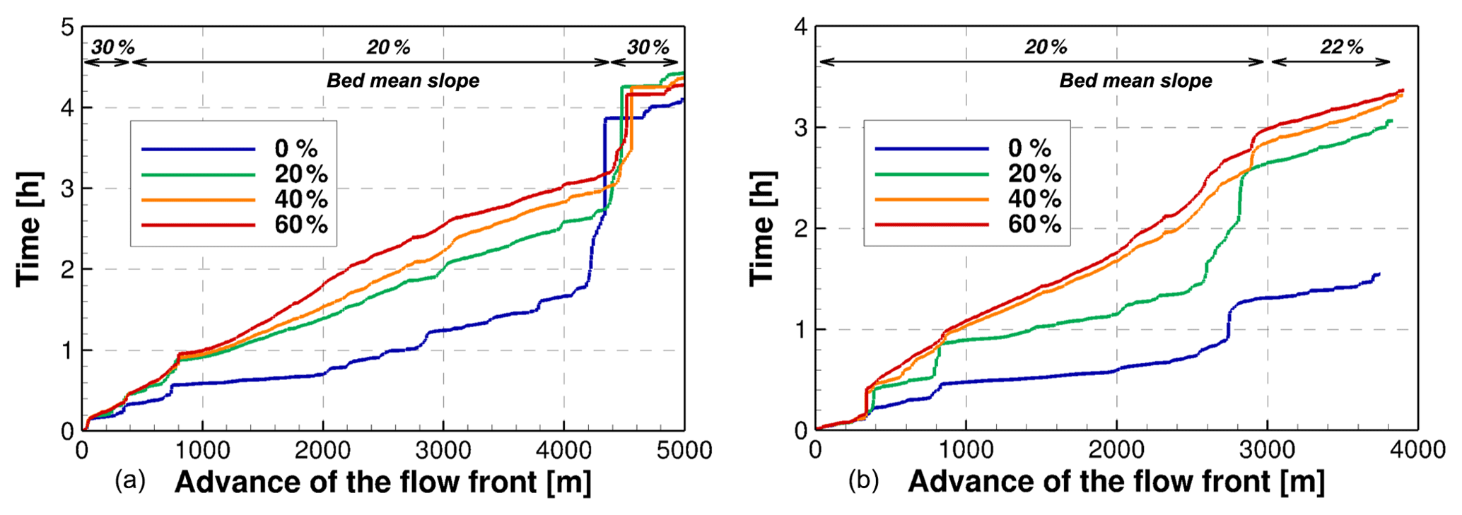
Figure 5Location of the wave front in time for both streams, considering four different sediment concentrations, to characterize the advance of the flood in the river: (a) Quebrada de Ramón and (b) Quillayes streams.
Figure 5 shows the location of the wave front vs. time for both streams upstream of the confluence. The inverse slopes of these curves represent the instantaneous velocity of the front for each sediment concentration we have simulated.
The numerical results show that the sediment concentration produces a significant change in the evolution of the flood, as it is the only factor that we modify in these simulations. The local variations in these velocities are produced by the gradual change of bed roughness and the slope of the river channels, which is approximately constant in large portions of the reaches. The Quillayes stream exhibits higher propagation velocities, which are also consistent with the steeper slopes and finer sediment diameters of the bed.
Figure 5 shows that the flood propagation has deceleration stages of the front, seen as steps in the location of the front in time. Two clear steps are observed in the Quebrada de Ramón stream. The first is located 800 m from the inflow boundary of the computational domain, which is produced by a local widening of the channel. The second deceleration, at 4500 m, is generated by a narrowing of the river that accumulates a large volume and reduces the velocity of the flow, increasing the depth upstream of this section due to backwater effects. In the Quillayes stream, we observe three deceleration stages at 400, 800, and 2800 m, which are also caused by local widening of the channel. These detailed dynamic features of the flood are modulated by the sediment concentration, as the hyperconcentrated cases show a more uniform propagation of the front.
Downstream of the confluence, we also observe the effects of the interaction between the morphology and the sediment concentration. The wave-front speed is affected by the different arrival times of flows from both tributaries. Figure 6 shows the distance traveled by the flood from the confluence to the outlet of the watershed. The origin is defined at the junction, and the time starts when the flood from the Quillayes, the faster and smaller stream, reaches the confluence. The time lapse between the arrivals is larger for flows with lower concentrations. This difference is equal to 3 h in clear-water flows, but only 1 h for a concentration of 60 %, which changes the hydrodynamics of the wave front when it arrives at the lower section of the channel, in the urban area. Along the first 4 km, we observe dynamics similar to those in Fig. 5, where the wave-front speed is faster as the flow is more diluted. Flows with high sediment concentration arrive at similar times at the confluence, such that the combination of flows from both streams propagates along the channel, keeping a faster wave-front velocity.
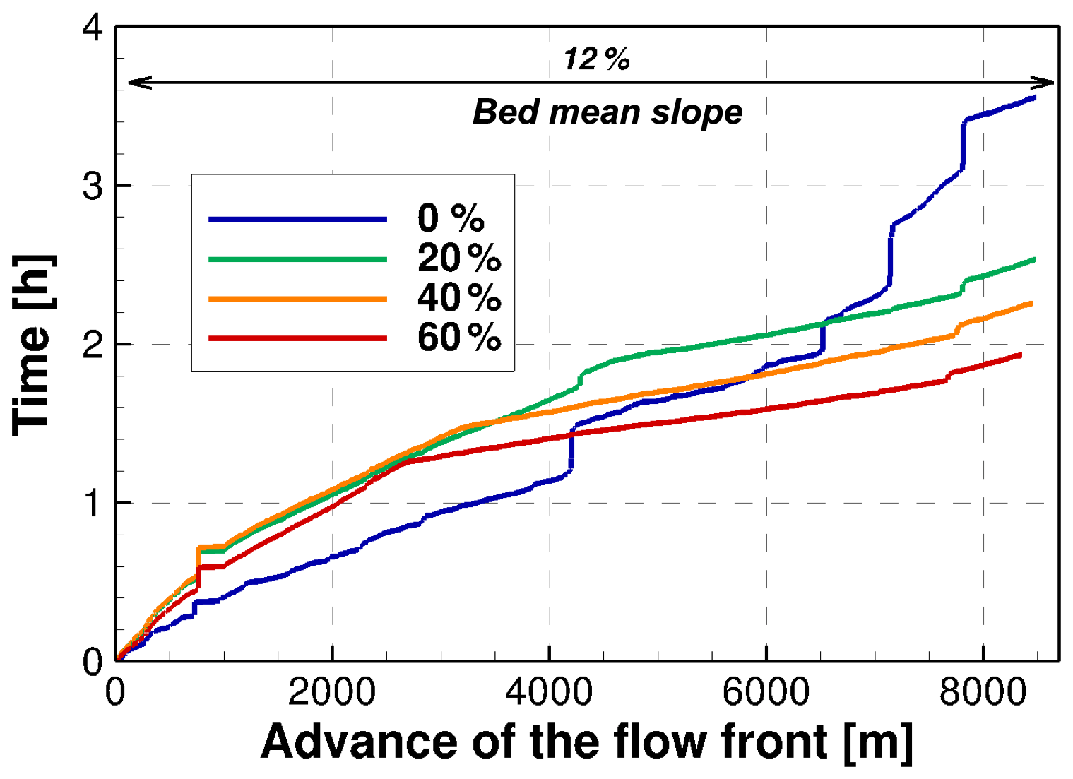
Figure 6Location of the wave front in time for the Quebrada de Ramón stream downstream of the confluence considering four sediment concentrations in both streams.
4.2 Peak flow and its arrival time
By comparing the hydrographs computed using different sediment concentrations at the four points monitored upstream of the confluence, we observe that the most important difference is the magnitude of the peak flow for different concentrations. The relative difference between the peak discharge simulated with clear-water flow compared to a sediment concentration of 60 % is 44 % at QR-U and 67 % at QR-D. To remove the effects of the additional volume that are produced by the sediment concentration in each stream, in Figs. 7 and 8 we show the normalized hydrographs, which are obtained by dividing the discharge by the total volume of the mixture that we obtain at each gauged point defined in Fig. 3. We can observe that the difference in the peak flows for different concentrations is only produced by the bulking effect of the sediments.
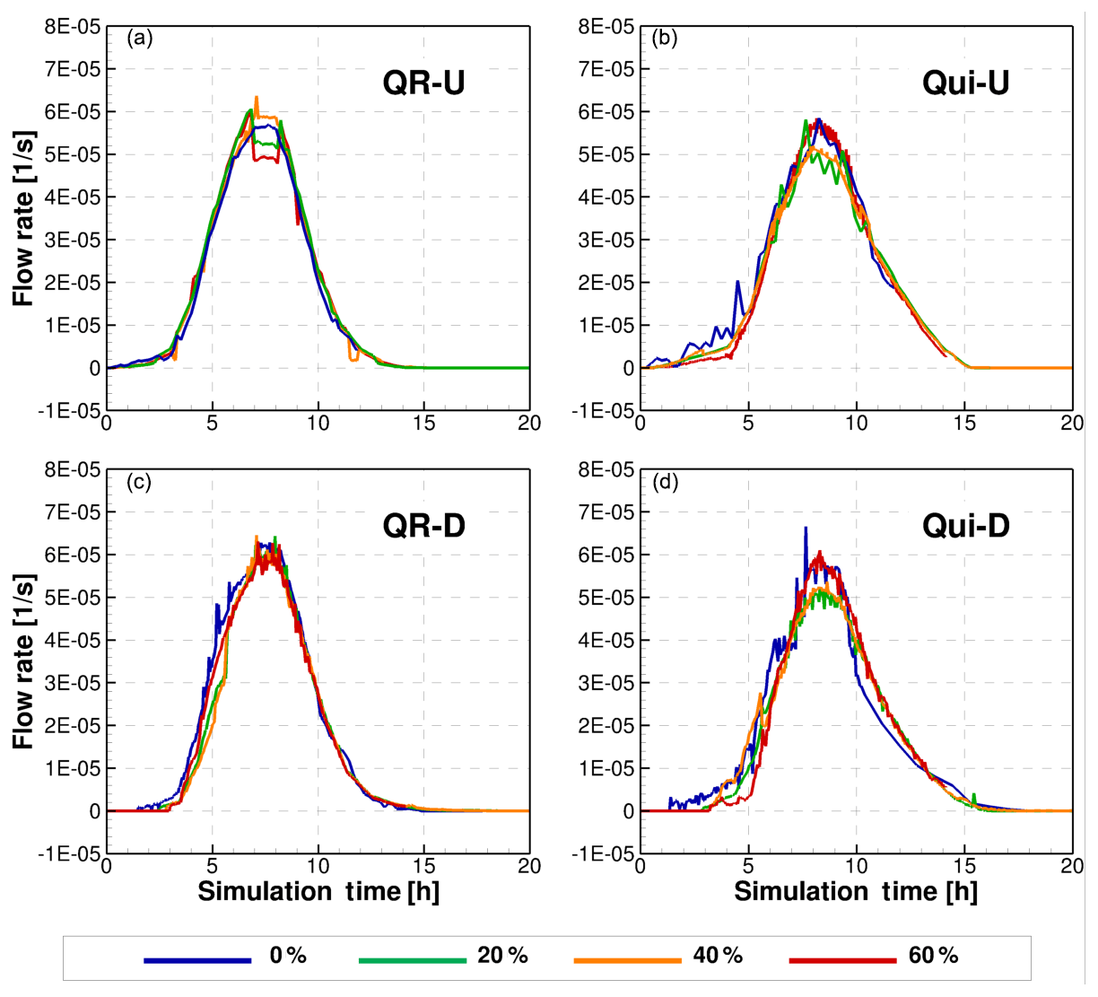
Figure 7Normalized hydrographs at the gauged points upstream of the confluence. In panels (a) and (c), we show the upper and lower zones in the Quebrada de Ramón stream, and panels (b) and (d) show the points at a similar elevation in the Quillayes stream.
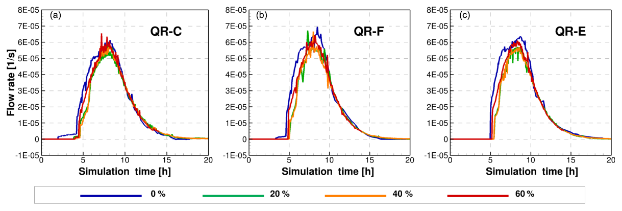
Figure 8Normalized hydrographs at the gauged points downstream of the confluence. In panel (a) we depict the point closest to the confluence, in panel (b) the flooding zone, and in panel (c) the outlet of the computational domain.
In both streams, the time to the peak of the hydrograph, however, is not significantly affected by the different concentrations. This seems to be related to the shape of the inflow hydrograph and to the location of the gauged points. The time to reach the peak discharge is around 7 h from the start of the simulation at QR-U, and 10 min later the maximum discharge reaches QR-D. At the Quillayes stream, the peak flow reaches Qui-U after 8 h from the start of the simulation, and Qui-D 13 min later.
When we analyze the hydrographs downstream of the confluence we observe similar results, as shown in Fig. 8. Due to the progressive reduction of the bed roughness, the peak flows increase in sections closer to the outlet of the watershed. The maximum peak flow is reached at the station QR-F, since the city park located at the north side of the main channel, and between QR-F and QR-E, is flooded and attenuates the peak flow near the outlet.
4.3 Total flooded area
The total area in the watershed that is inundated for different sediment concentrations is depicted in Fig. 9. No significant differences are noticed for most of the length of the river channel. Both streams have steep slopes in confined canyons, and the maximum flow depth, reaching up to 3 m, does not significantly alter the horizontal extension of the 2-D area affected by the flood.
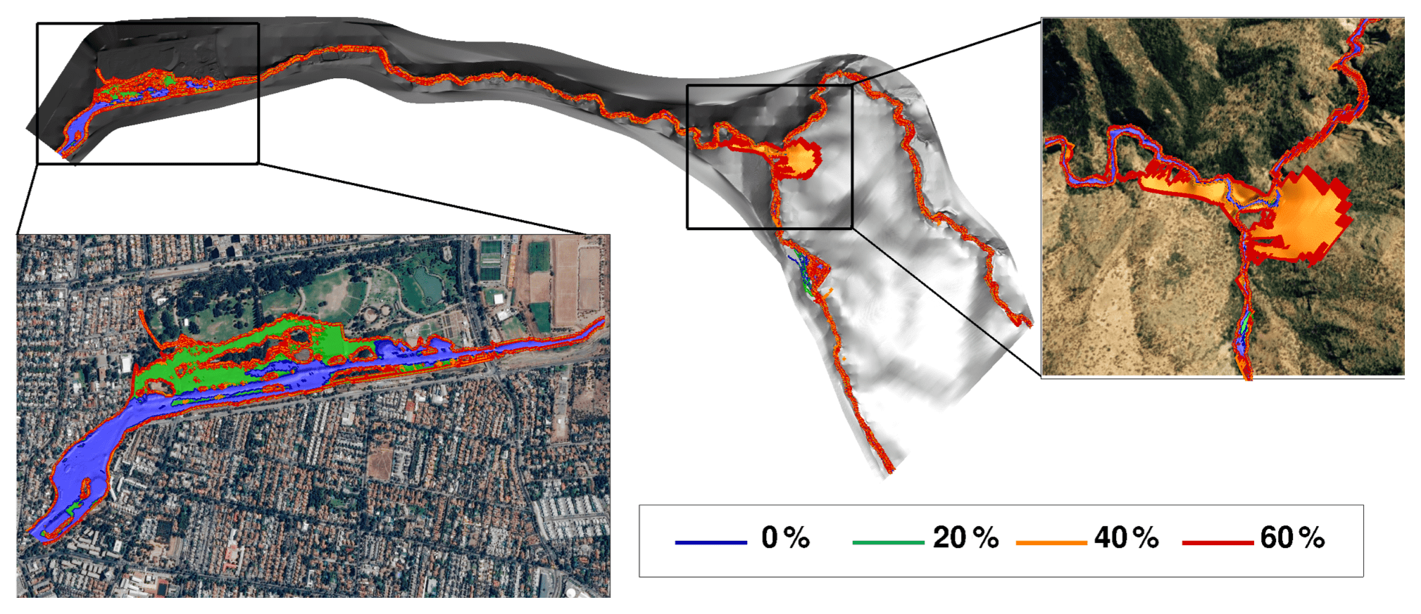
Figure 9Contours of the flooded area for different sediment concentrations along the channel, and in the city of Santiago. Image of the terrain from © Google Earth.
Major differences, however, appear in regions with milder slopes, around the confluence and in the city, near the outlet of the watershed. At the confluence, simulations with higher concentrations of 40 % and 60 % overflow the natural channels, due to the fast arrival of a large volume of water and sediment flow to this region. In the city, near the outlet of the domain, all the flows inundate the urban park located at the north bank of the main channel, downstream of a large urbanized area. In this section, the most important increment of the total flooded area occurs when we increase the concentration from clear water to 20 %, where the total flooded area increases by 36 %. For larger concentrations the affected area grows gradually compared to the clear-water flooding case, as the fluid is more concentrated. Increments of the total area of 46 % and 75 % are observed for concentrations of 40 % and 60 %, respectively.
4.4 Maximum flow depth and mean velocity
Figure 10 shows the maximum depth registered at each gauged point along the channels for the different sediment concentrations we simulate. The numerical results show that the depth increases with concentration, and the largest differences are obtained between the clear-water case and 20 % concentration, at six of the measurement points we analyze. In QR-C for instance, the first increment of the sediment concentration, from clear water to 20 %, produces a maximum depth that is 24.1 % larger, whereas increasing the concentration from 20 % to 40 %, and then to 60 %, the flow depth increases in only 7.5 % and 5.1 %.
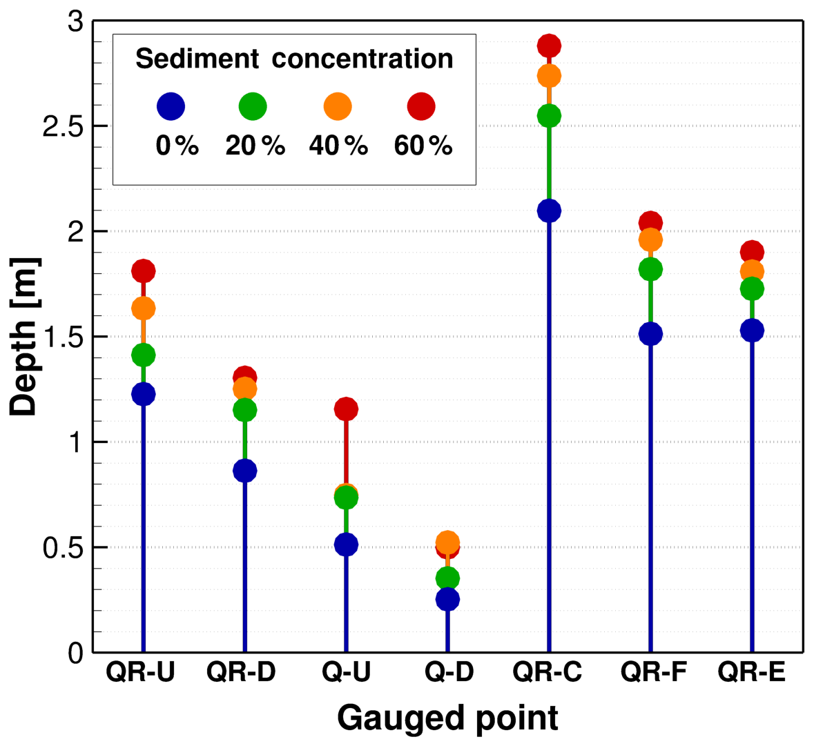
Figure 10Maximum depth computed at every gauged point depending on the sediment concentration.
By comparing the flow depths in the simulations, we note that the deepest flow is always located downstream of the confluence (QR-C). At this location, a difference of 0.80 m is measured between the clear water and the flow with the maximum concentration of 60 %. In the urban areas (points QR-F and QR-E), depths larger than 2 m are observed. Here, it is important to have a precise solution for different sediment concentrations since there is a difference of 0.5 m between clear water and the maximum concentration, which can have significant impacts on the design of flood control measures.
Additionally, in Fig. 11 we show the mean velocity at each measurement point for the range of sediment concentrations. In this case, we cannot observe a clear trend of velocity changes as a function of concentration. For this flow variable, it seems that the local topographic conditions considerably affect the averages of the flow hydrodynamics.
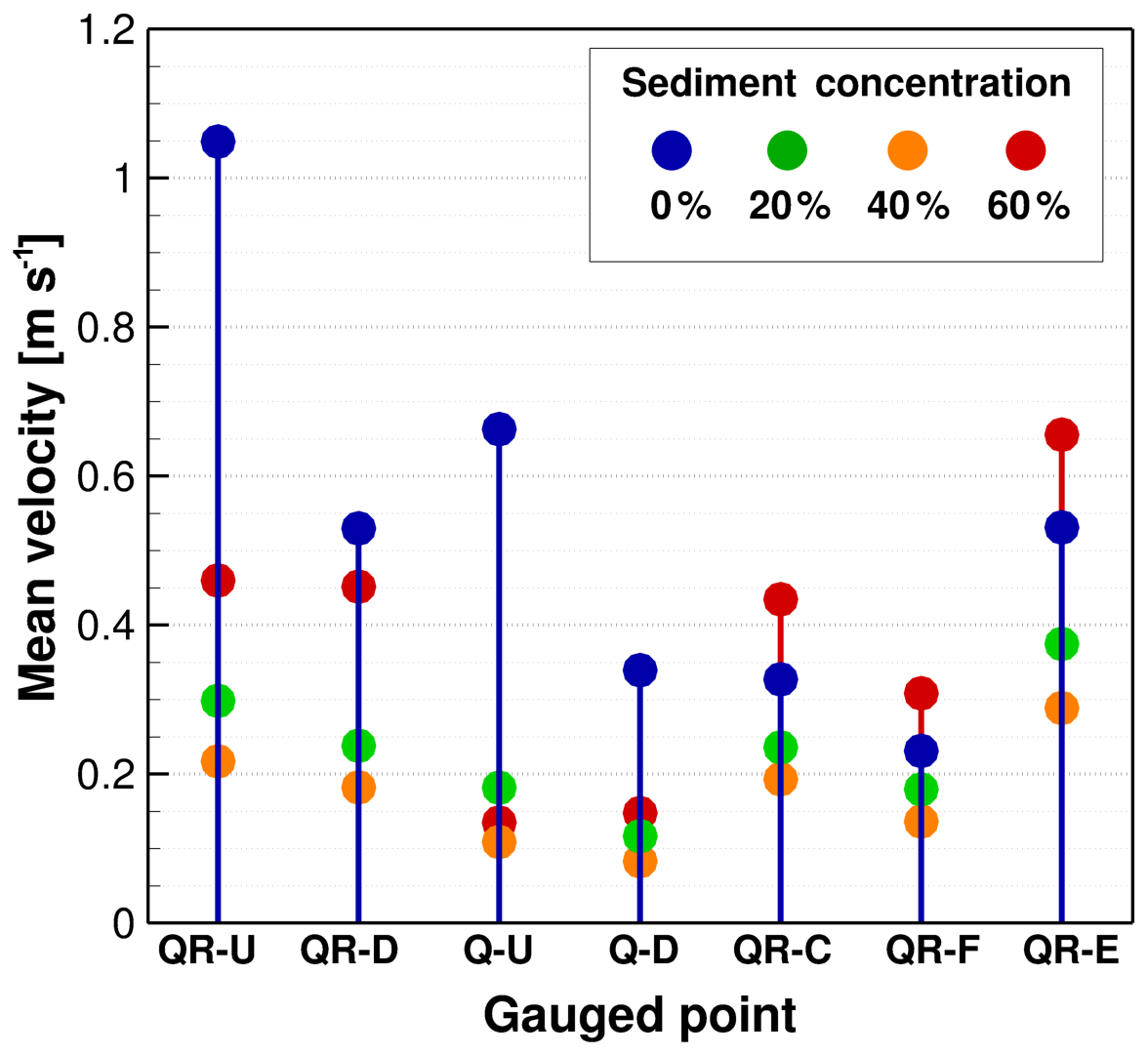
Figure 11Mean velocity computed at each gauged point depending on the sediment concentration.
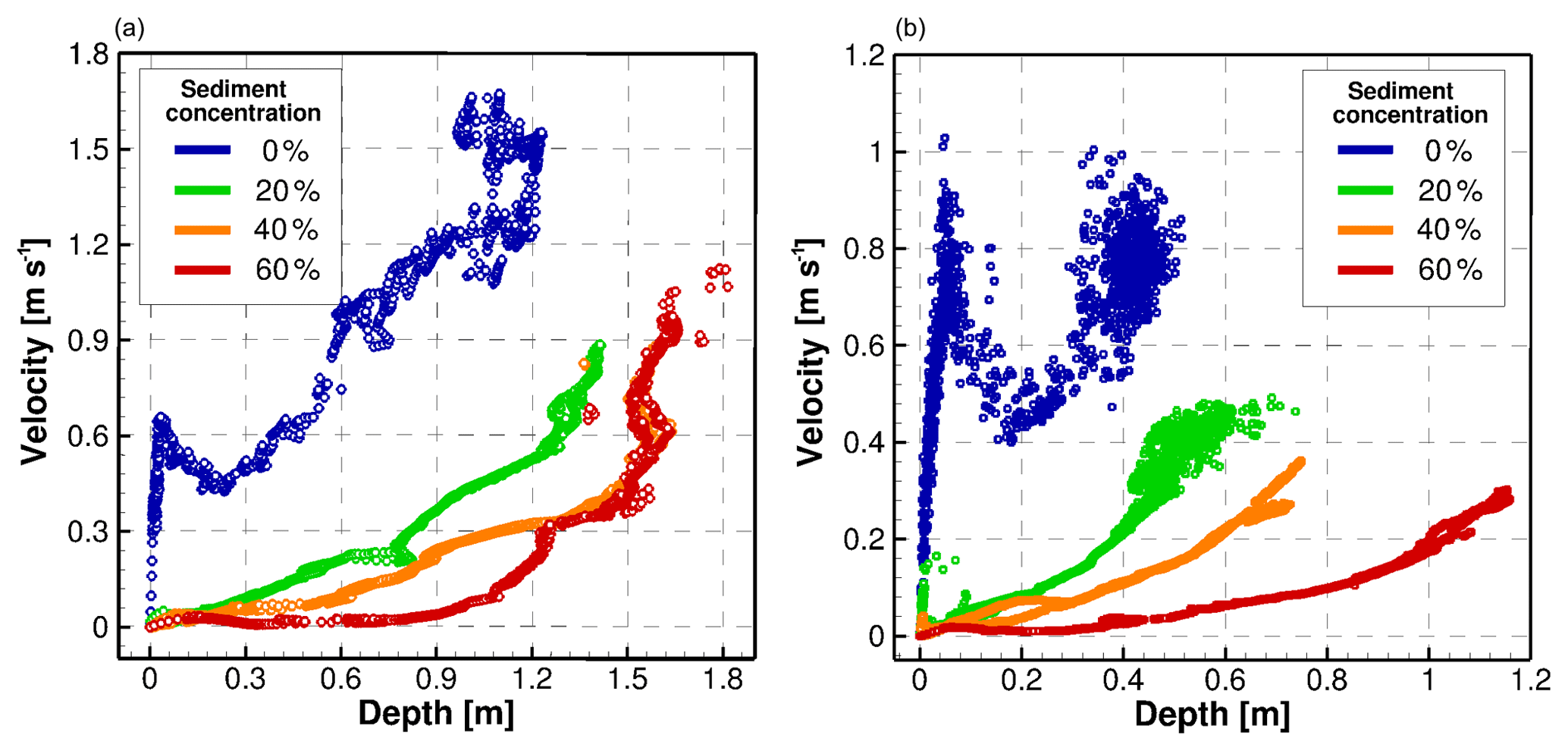
Figure 12Stage–velocity relation between the computed flow depths and velocities for different sediment concentrations. The data at the point QR-U are shown in panel (a) and Qui-U in panel (b).
In Fig. 12 we relate the magnitude of the hydrodynamic variables, velocity vs. depth, computed at each time step at QR-U in panel (b) and Qui-U in panel (a). These plots are similar to a stage–velocity relation that links the flow depth and the total velocity at the same instant in time. The plots are constructed using data every 30 s, for a total time of 24 h.
Even though a direct relation is not observed between mean velocity and sediment concentration at points QR-U and Qui-U (Fig. 11), the depth–velocity plots in Fig. 12 confirm the relation of large depths and lower velocities as the concentration increases. This is closely related to the changes in the flow resistance. Larger concentrations increase the yield stress, the fluid viscosity, and the dispersive effects, producing additional momentum losses, which reduce the flow velocity. The stage–velocity relation is different for clear-water flow compared to the sediment-laden cases. For hyperconcentrated flows, the relationship between the depth and velocity is fitted to a quadratic regression that always increases. In clear water the relation is linear in shallow flows under 0.05 m deep, where the Froude number is larger than 1, reaching 1.43 and 1.53 at QR-U and Qui-U, respectively. Then, a transition zone with depths between 0.05 and 0.2 m and an almost critical Froude number is observed. Above 0.2 m depth, the velocity increases quadratically as seen in the flows with higher sediment concentrations. In this zone, the flow is dominated by gravity with subcritical Froude numbers of around 0.25.
4.5 Flow momentum in the urban area
To evaluate the potential damage to the infrastructure generated by floods, we can compute the flow momentum at each cross section of the flooded area. In this case we compare the maximum force produced by the flow in the urban area of the watershed, considering flows with different sediment concentrations coming from the Quebrada de Ramón and the Quillayes streams. Figure 13 shows contours of maximum cross-section momentum along the river. The top figure shows the momentum for a sediment concentration of 20 % in the Quebrada de Ramón stream and 60 % in the Quillayes stream. The opposite case, 60 % in the Quebrada de Ramón stream and 20 % in the Quillayes stream, is depicted in Fig. 13b.
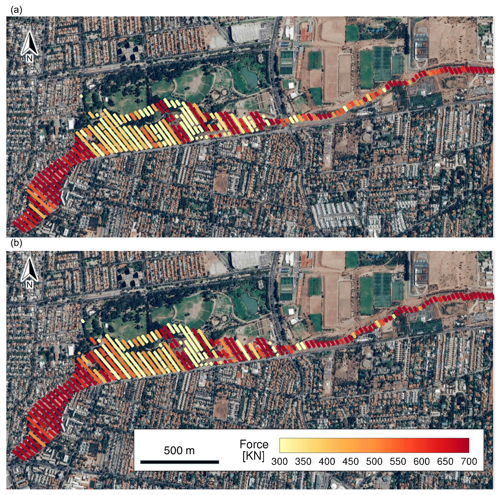
Figure 13Maximum momentum of the flow in the urban area. Panel (a) shows results for a concentration of 20 % coming from the Quebrada de Ramón stream and 60 % from the Quillayes stream. Panel (b) corresponds to the opposite case, 60 % from the Quebrada de Ramón stream and 20 % from the Quillayes stream. Image of the terrain from © Google Earth.
The approaching flow has an approximate force of 700 kN in both simulations. For these two cases, the areas with the highest momentum correspond to (1) the confined zone in the right of the image and (2) at the outlet of the basin in the urban area. However, the force is on average 14.5 % higher in the second case, which could be related to the higher flow density of the flow that is obtained downstream of the confluence.
Since the density in these simulations is different in both streams upstream of the confluence, the density of the fluid in the main channel varies in time and space, both along and across the flow. The mean concentration in the main channel, downstream of the confluence, is around 30 % and 44 % considering a sediment concentration of 20 % in the Quebrada de Ramón stream and 60 % in the Quillayes stream and vice versa, respectively. These values are consistent with the theoretical concentrations computed from the fully mixed conditions.
The results evidence the competition between two main factors that control the dynamics of the flow in mountain rivers at different spatial and temporal scales: (1) the geomorphological features of the river represented by the bathymetry, the slope, and the channel width and (2) the flow resistance due to the internal sediment dynamics that changes the rheology of the mixture.
At timescales of seconds or minutes, flow velocities and depths along the channel are significantly affected by both factors, having a great impact on global variables such as the wave-front velocity, the total inundated area, and the cross-section momentum of the flow. As reported in Sect. 4.1, the mean velocity of the wave front is reduced as the sediment concentration increases, which is produced by flow resistance driven by the dispersive stresses of the sediment. The flow depth is increased by these higher momentum losses and by the bulking effect of the additional sediment mass, resulting in a direct impact on the increment of the flooded area and flow momentum in the city. We also observe discontinuities in the advance of the flow front in time, which are located in the vicinity of sudden changes of slope or channel width that are common in mountain canyons in the Andes. Local changes of sediment concentration can even suppress geomorphic effects, having large-scale impacts on the flood propagation, as the sediment concentration can change the flow regime from supercritical to subcritical, as shown in Fig. 12.
Global bulk variables, on the other hand, such as the normalized hydrograph shape and the time to the peak discharge, show a geomorphic control at the scales of the duration of the entire event. Except in areas where there is a change in the flow regime, the effects of the sediment concentration are not observed for the time-averaged velocities along the channel. As shown in the normalized plots in Fig. 7, however, the differences in the arrival time of the peak flow are of the order of minutes, which is small compared to the entire duration of the flood hydrograph with a total of 20 h.
It is important to point out that the sensitivity of the flow physics affected by the sediment concentration, such as the mean velocity of the wave front, flow depth, instantaneous velocity, flooded area, and flow momentum, decreases for higher sediment concentrations. We show that as the sediment concentration increases, the changes are more significant in the range between 0 % and 20 %, compared to the flood propagation for increments over 40 %. These new insights are relevant to determine flood hazard in mountain rivers and define a reduced number of possible scenarios for different concentrations in these rivers.
The primary emphasis of this work is to examine the effects of the sediment concentration on the flood dynamics in an Andean watershed. To simulate different scenarios, we developed a finite-volume numerical model that solves the hydrodynamics of hyperconcentrated fluids in complex natural topographies. The model is based on the work of Guerra et al. (2014), and it is employed to solve the nonlinear shallow water equations coupled to a transport equation for the sediment in generalized curvilinear coordinates. To consider the effects of the sediment concentration, we implement a new version of the quadratic rheological model (O'Brien et al., 1993) to calculate the stresses produced by high concentrations, separating the turbulent and dispersive effects of the sediment concentration.
To investigate the effects of the sediment concentration in floods that occur in mountain rivers, we perform simulations in the Quebrada de Ramón watershed, an Andean catchment located in central Chile. We analyze the changes in hydrodynamic variables such as peak discharge, arrival time of the flood wave, cross-section momentum, flow depth, mean velocity, and total flooded area. Most of the these results are compared and analyzed in seven points along the channel.
The most important effects on the flood propagation are observed for the increments of sediment concentration just above the clear-water flow, in the range of concentrations from 0 % to 20 %. Even though the channel slope is the most important morphological feature that controls the dynamics of the flow, local factors such as channel widening can significantly change the propagation of the flood wave. High sediment concentrations modulate these morphodynamic effects, producing larger flow depths and slower velocities overall.
Some of the hydrodynamic variables analyzed were more sensitive to changes in sediment concentration. We observed significant effects on the total flooded area and momentum of the flow as the flood arrives at the urban area. While the extent of the 2-D flooded area in the entire basin remains more or less constant for different concentrations, the largest difference is observed in the city, where the slopes are milder. The simulations show a difference of 76 % in the total 2-D flooded area when we compare the clear-water conditions with the 60 % concentration. Regarding the cross-section momentum as the flood advances in the urban zone, we show that the maximum momentum of the flow increases 14 % on average for a 20 % concentration in the Quebrada de Ramón stream and a 60 % concentration in the Quillayes stream. We also observe that bulk variables, such as the arrival time of the peak discharge at different locations of the basin, and the shape of the hydrograph are not modified significantly with the magnitude of the sediment concentration, but they are associated with the local morphological conditions of the river channel.
The numerical solution of the system of Eq. (5) is based on the method developed by Guerra et al. (2014) to solve the NSWE, which has shown great efficiency and precision in simulating extreme flows and rapid flooding over natural terrains and complex geometries. This is a finite-volume formulation that is implemented in two steps: first, in the so-called hyperbolic step, the Riemann problem is solved at each element of the discretization without considering momentum sinks. The flow is reconstructed hydrostatically from the bed slope source term, adding the effects of the spatial concentration gradients. In the second step we incorporate the shear stress source terms by means of a semi-implicit scheme, correcting the predicted values of the hydrodynamic variables obtained in the previous step.
The initial hyperbolic step consists of numerically solving the following equation:
in which a semi-discrete finite-volume formulation in generalized curvilinear coordinates can be written as follows:
where Qi,j and Ji,j represent the vector of hydrodynamic variables and the Jacobian of the coordinate transformation at the center of the discrete elements of the grid (i,j). The vectors and are the numerical fluxes through each of the cell interfaces. The terms Δξ and Δη correspond to the size of the discretization, and and are the discrete source terms of the bed slope and concentration gradients, respectively.
To compute the numerical fluxes we implement the VFRoe-ncv method (Gallouët et al., 2003; Marche, 2006) to solve Eq. (A1), through a nonconservative change of variables, linearizing the Riemann problem (Guerra et al., 2014). The vector of hydrodynamic variables Qi,j is extrapolated to the boundaries of each cell to ensure the non-negativity of the intermediate states and flow depths, preserving the dry zones of the terrain. The monotonic upwind scheme for conservation laws (MUSCL) method, developed by Van Leer (1979), is used to perform the extrapolation with 2nd-order accuracy. Finally, the methodology developed by Masella et al. (1999) is used to avoid unphysical solutions due to the lack of dissipation to capture shock waves.
The bed-slope source term is computed following the well-balanced methodology developed by Audusse et al. (2004) and adapted to generalized curvilinear coordinates by Guerra et al. (2014). This method hydrostatically reconstructs the free surface by performing a balance between the topographic variations in the domain and the hydrostatic pressure. The hydrodynamic variables and bed elevations are extrapolated to the boundaries of the cells using the MUSCL method, locally and globally preserving the dry zones and stationary steady states. To ensure the non-negativity of the flow depth and to avoid spurious oscillations, the minmod limiter is implemented during the hydrostatic reconstruction of the fluid depth, such that realistic values of the spatial gradients of depth are reached in the shock waves (LeVeque, 2002; Bohorquez and Fernandez-Feria, 2008).
The concentration gradient term is discretized using the following scheme:
where hi,j and Ci,j are the centered-cell flow depth and sediment concentration, respectively, and and are the sediment concentrations at the interfaces of the each cell, obtained from a 1st-order upwind scheme.
In the second step of the numerical solution, we incorporate the momentum source terms in vector SS(Q), solving the following system of equations:
We use a splitting semi-implicit method (Liang and Marche, 2009), employing a 2nd-order Taylor expansion. The limiters developed by Burguete et al. (2007) are implemented to avoid numerical instabilities at the wet–dry interfaces, where the flow depths are shallower. These limiters are designed to prevent unphysical effects, such as reversed flows due to high shear stresses.
Finally, the temporal integration of Eq. (A1) is carried out by using a 4th-order Runge–Kutta numerical scheme. The condition for numerical stability of the model is based on the Courant–Friedrichs–Lewy (CFL) criterion.
The boundary conditions are handled by creating two rows of “ghost cells” outside of the computational domain (Sanders, 2002). We implement three types of boundaries: (1) open or transmissive boundary at the outlets, (2) closed reflective boundary for the solid walls, and (3) inflow boundary to introduce a hydrograph or a controlled discharge toward the computational domain.
B1 Quiescent equilibrium in a tank
This benchmark test is developed to demonstrate the capacity of the model to preserve the hydrostatic state with density differences. An analytical solution is obtained from the procedure developed by Leighton et al. (2010), in which the original system of Eqs. (1) to (4) is simplified by considering steady flow () and a stationary initial state () in inviscid flow with zero stresses (). Therefore, the equations are reduced to
which can be written as follows:
Hence, for a rectangular tank of length L and width A, with a constant initial flow depth and a bed described by a cosine function,
and the analytical solution of Eq. (B2) becomes
where ρ0 is the initial reference value of the fluid density.
The dimensions and initial conditions of this test are presented in Fig. B1, where the reference density ρ0 was set to 1000 kg m−3. The 1-D computational domain was discretized in a grid of 1001 cells in the longitudinal direction, with a reflective solid wall boundary condition at each wall of the tank. The total simulated time was 100 s and the CFL number was set to 0.2.
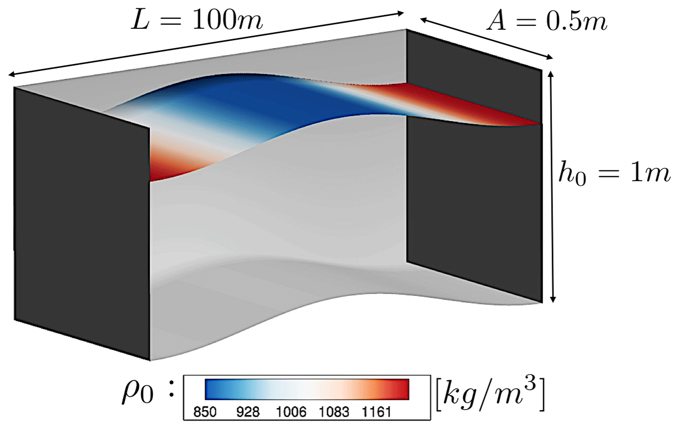
Figure B1Dimensions and initial conditions of the rectangular tank used for the quiescent equilibrium test (Leighton et al., 2010).
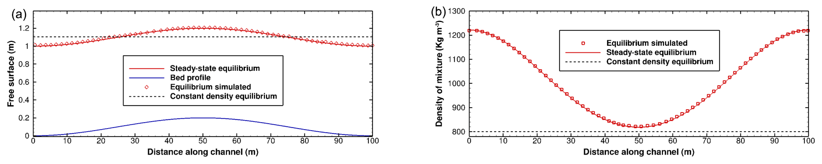
Figure B2Quiescent equilibrium test. Comparison between theoretical and numerical profiles of hydrodynamic variables. (a) Free surface and (b) fluid density.
Results show that there is an excellent agreement between the analytical and numerical solutions for the free surface, as shown in Fig. B2a and the density profile in Fig. B2b. The maximum error of water depth is equal to 10−7 m, and the model is capable of maintaining the steady state of the flow.
B2 Density dam break with two initial discontinuities
To test the model in unsteady conditions, we simulate a density-driven dam break to evaluate the evolution of the hydrodynamic variables in space and time. The numerical experiment is based on the work developed by Leighton et al. (2010), which consists of a horizontal rectangular tank of 100 m long, with two fluids of different densities ρ1 and ρ2, as shown in Fig. B3. The acceleration of gravity is considered equal to 1 m s−2, and the shear stresses are neglected.
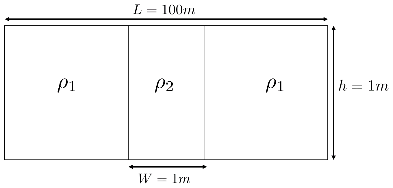
Figure B3Initial state of the density-driven dam break (Leighton et al., 2010).
Two different simulations are performed for ρ2=0.1 kg m−3 and ρ2=10 kg m−3, while ρ1 is kept constant and equal to 1 kg m−3. Both simulations are implemented on a regular grid with a resolution of 0.005 m for 30 s, using a CFL=0.2 and reflective boundary conditions at solid walls.
In Fig. B4 we show the instantaneous flow depth and velocity profiles at 2 and 30 s, from the start of the first simulation (ρ2=0.1 kg m−3). A good agreement is found with respect to the solution provided by Leighton et al. (2010), as we capture the propagation of the free surface and velocity magnitudes that are generated by the initial imbalance of the hydrostatic pressure at the interface of the fluids. The amplitudes of the main shock are slightly smaller due to the 2nd-order accuracy of the numerical model. Similar results are obtained for ρ2=10 kg m−3 as shown in Figs. B5 and B6, which also show that the model can resolve sharp gradients, and the solutions do not change significantly with the grid resolution.
Note that when , the flow velocities are directed toward the middle of the tank, where the fluid is less dense, which increases the flow depth in that zone. Conversely, when , the fluids move to reach hydrostatic equilibrium, balancing the pressure in the entire domain, which produces higher depths at the sidewalls.
B3 Large-scale experimental dam break
To test the rheological model, we simulate the large-scale dam-break experiment with high sediment concentration performed by Iverson et al. (2010). We compare the numerical results with the measurements of flow depth and the arrival time of the wave front. It is important to note that the simulation of this experiment is a very challenging computational test for the numerical model. The slope of the channel, the sediment concentration, and the flow phenomena as the wave advances generate a complex dynamic that is difficult to measure and reproduce with a high-resolution numerical model.
The experiment consists of the sudden release of a large volume of a sediment–water mixture in a 95 m long rectangular channel, with a cross section that is 2 m wide by 1.2 m deep. The channel is very steep, with an inclination of 31∘ for the first 75 m downstream from the gate and 2.5∘ for the downstream section. The total volume released in the dam-break experiment is 6 m3, with an initial depth of 2 m and a volumetric sediment concentration of 64.7 %. The bed roughness changes along the channel, with a representative roughness height of 1 mm for the first 6 m of the channel measured from the gate and a roughness of 15 mm in the rest of the channel, downstream. The sediment density considered in this case is ρs=2700 kg m−3.
The unsteady inflow condition is the debris flow at a distance of 2 m downstream from the gate, which is shown in Fig. B7. This was obtained from the simulation of the dam break delayed 1 s to consider the delay of the opening of the gate, as reported by Iverson et al. (2010). We simulate a total time of 25 s, using a 2-D spatial discretization with a uniform resolution of 0.1 m and a CFL number equal to 0.1.
In Fig. B8 we compare the flow thickness between the simulation and the experiment at two locations, corresponding to 32 and 66 m downstream of the gate. The experimental data were collected by Iverson et al. (2010) at a frequency of 100 Hz. In our simulation, the grid is fine enough to resolve the well-known roll waves that appear at high Froude numbers in steep channels (Bohorquez and Fernandez-Feria, 2006). This phenomenon has also been recently observed in the simulations of the same experiment by Bohorquez (2011). In this case we capture roll waves with an amplitude close to 0.5 m, as shown by the red line in Fig. B8.
To compare the numerical results directly with data provided by the experiments, we apply the same moving-average filter used to smooth the experimental data (black line in Fig. B8). The model reproduces with good agreement the arrival time of the wave front in both gauges, with delays smaller than 0.2 s. The maximum flow depth computed at the location of 32 and 66 m downstream from the gate is over- and underestimated by just 1.78 and 1.6 cm, respectively.
The simulated and observed wave-front positions in time are very similar (Fig. B9) with values of the mean square error and the coefficient of determination of the fit being 1.98 m and R2=99.28 %, respectively. The sudden discontinuity in the computed front velocity at 7.6 s is due to a roll wave advancing through the front, which briefly slows down the flow. Due to the resolution of the experimental results, we cannot directly compare this phenomenon captured in the simulation.
Overall, the validation study shows that the numerical model in these extreme cases is very robust and it is able to reproduce many of the phenomena of interest that appear in hyperconcentrated flash floods.

Figure B4Density-driven dam break. Case ρ2=0.1 kg m−3: comparison of the flow depth (a, c) and velocity profiles (b, d) at (a, b) s and (c, d) s from the beginning of the simulation.

Figure B5Density-driven dam break. Case ρ2=10 kg m−3: comparison of the flow depth at , 4, 12, and 30 s from the beginning of the simulation.
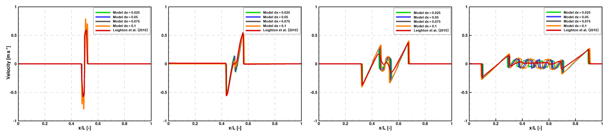
Figure B6Density driven dam break. Case ρ2=10 kg m−3: comparison of velocity profiles at , 4, 12, and 30 s from the beginning of the simulation.

Figure B7Unsteady inflow boundary condition corresponds to the cross-section flow measured at a location of 2 m downstream of the gate (Iverson et al., 2010).
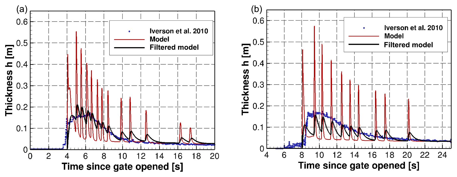
Figure B8Comparison of the flow thickness measured in the experiment of Iverson et al. (2010) and computed with our model. Flow thickness at two locations: (a) 32 m and (b) 66 m downslope from the gate.
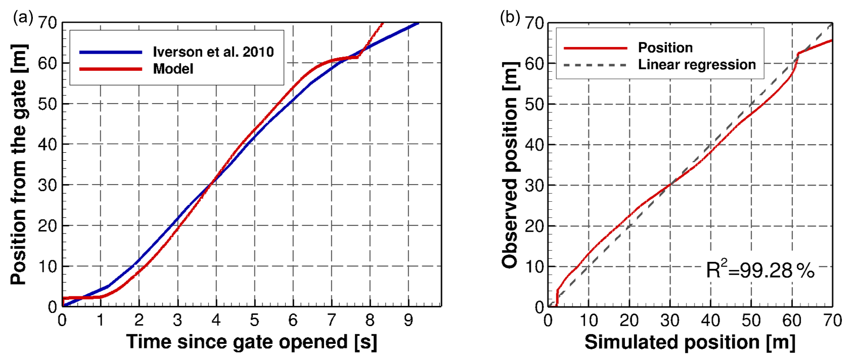
Figure B9Comparison of the position of the flow front as a function of time: (a) the position of the flow front over the time and (b) comparison of the experimental and simulated flow front position. The dashed line is the perfect fit with a slope equal to 1.
The code and data are available at https://doi.org/10.5281/zenodo.3597889 (Contreras, 2020).
MTC and CE conceived the study, analyzed the data, interpreted the results, and wrote the paper. MTC developed the numerical code and performed the simulations for the cases presented in the paper, under the supervision of CE.
The authors declare that they have no conflict of interest.
This article is part of the special issue “Advances in computational modelling of natural hazards and geohazards”. It is a result of the Geoprocesses, geohazards – CSDMS 2018, Boulder, USA, 22–24 May 2018.
This work has been supported by Conicyt/Fondap grant 15110017. This research has been partially supported by the supercomputing infrastructure of the NLHPC (ECM-02). Additional funding from VRI of the Pontificia Universidad Católica de Chile, internationalization of research, project PUC1566, MINEDUC. We thank the Ministry of Public Works for providing the lidar topography. Verónica Ríos and Jorge Gironás provided the flood hydrographs.
This research has been supported by the CONICYT/FONDAP (grant no. 15110017) and the VRI internationalization of research, MINEDUC (grant no. PUC1566).
This paper was edited by Albert J. Kettner and reviewed by two anonymous referees.
Anastasiou, K. and Chan, C.: Solution of the 2D shallow water equations using the finite volume method on unstructured triangular meshes, Int. J. Numer. Meth. Fl., 24, 1225–1245, 1997. a
Ancey, C.: Plasticity and geophysical flows: A review, J. Non-Newton. Fluid, 142, 4–35, https://doi.org/10.1016/j.jnnfm.2006.05.005, 2007. a
Arnell, N. and Gosling, S.: The impacts of climate change on river flood risk at the global scale, Climatic Change, 134, 387–401, https://doi.org/10.1007/s10584-014-1084-5, 2014. a
Audusse, E., Bouchut, F., Bristeau, M., Klein, R., and Perthame, B.: A fast and stable well-balanced scheme with hydrostatic reconstruction for shallow water flows, SIAM J. Sci. Comput., 25, 2050–2065, 2004. a
Bagnold, R.: Experiments on a gravity-free dispersion of large solid spheres in a Newtonian fluid under shear, P. Roy. Soc. A-Math. Phy., 225, 49–63, https://doi.org/10.1098/rspa.1954.0186, 1954. a, b, c
Bankoff, G., Frerks, G., and Hilhorst, D.: Mapping vulnerability: Disasters, Development and People, Routledge, https://doi.org/10.4324/9781849771924, 2004. a
Bathurst, J.: Flow resistance of large-scale roughness, J. Hydr. Div., 104, 1587–1603, 1978. a
Bingham, E.: Fluidity and plasticity, McGraw-Hill New York, New York, USA, 1922. a
Blaikie, P., Cannon, T., Davis, I., and Wisner, B.: At risk: Natural hazards, people's vulnerability and disasters, Routledge, London, UK, 2004. a
Boers, N., Bookhagen, B., Barbosa, H., Marwan, N., Kurths, J., and Marengo, J.: Prediction of extreme floods in the eastern central Andes based on a complex networks approach, Nat. Commun., 5, 1–7, https://doi.org/10.1038/ncomms6199, 2014. a
Bohorquez, P.: Discussion of “Computing nonhydrostatic shallow-water flow over steep terrain” by Roger P. Denlinger and Daniel R. H. O'Connell, J. Hydraul. Eng., 137, 140–141, https://doi.org/10.1061/(asce)0733-9429(2008)134:11(1590), 2011. a
Bohorquez, P. and Fernandez-Feria, R.: Nonparallel spatial stability of shallow water flow down an inclined plane of arbitrary slope, River Flow, 1, 503–512, 2006. a
Bohorquez, P. and Fernandez-Feria, R.: Transport of suspended sediment under the dam-break flow on an inclined plane bed of arbitrary slope, Hydrol. Process., 22, 2615–2633, 2008. a
Burguete, J., García-Navarro, P., and Murillo, J.: Friction term discretization and limitation to preserve stability and conservation in the 1D shallow-water model: Application to unsteady irrigation and river flow, Int. J. Numer. Meth. Fl., 58, 403–425, https://doi.org/10.1002/fld.1727, 2007. a
Cao, Z., Pender, G., Wallis, S., and Carling, P.: Computational dam-break hydraulics over erodible sediment bed, J. Hydraul. Eng., 130, 689–703, 2004. a
Contreras, M. T.: Modeling the effects of sediment concentration on the propagation of flash floods in an Andean watershed – Code, Zenodo, https://doi.org/10.5281/zenodo.3597889, 2020. a
D'Aniello, A., Cozzolino, L., Cimorelli, L., Della Morte, R., and Pianese, D.: A numerical model for the simulation of debris flow triggering, propagation and arrest, Nat. Hazards, 75, 1403–1433, https://doi.org/10.1007/s11069-014-1389-8, 2015. a
Díaz, H. and Markgraf, V.: El Niño: Historical and paleoclimatic aspects of the Southern Oscillation, Cambridge University Press, Cambridge, UK, 1992. a
European Environmental Agency (EEA): Vulnerability and adaptation to climate change in Europe, EEA Technical Report No. 7, Luxembourg, 2005. a
Eyring, H.: Statistical Mechanics and Dynamics, Wiley, New York, USA, 1964. a
Gallouët, T., Hérard, J., and Seguin, N.: Some approximate Godunov schemes to compute shallow-water equations with topography, Comput. Fluids, 32, 479–513, https://doi.org/10.1016/S0045-7930(02)00011-7, 2003. a
Guerra, M., Cienfuegos, R., Escauriaza, C., Marche, F., and Galaz, J.: Modeling rapid flood propagation over natural terrains using a well-balanced scheme, J. Hydraul. Eng., 140, 04014026, https://doi.org/10.1061/(ASCE)HY.1943-7900.0000881, 2014. a, b, c, d, e, f, g, h
Hirabayashi, Y., Mahendran, R., Koirala, S., Konoshima, L., Yamazaki, D., Watanabe, S., Kim, H., and Kanae, S.: Global flood risk under climate change, Nat. Clim. Change, 3, 816–821, https://doi.org/10.1038/nclimate1911, 2013. a
Holton, J., Dmowska, R., and Philander, S.: El Niño, La Niña, and the Southern Oscillation, Academic press, https://doi.org/10.1016/S0074-6142(08)60170-9, 1989. a
Iverson, R., Logan, M., La Husen, R., and Berti, M.: The perfect debris flow? Aggregated results from 28 large-scale experiments, J. Geophys. Res., 115, F03005, https://doi.org/10.1029/2009JF001514, 2010. a, b, c, d, e
Jongman, B., Ward, P., and Aerts, J.: Global exposure to river and coastal flooding: Long term trends and changes, Global Environ. Chang., 22, 823–835, https://doi.org/10.1016/j.gloenvcha.2012.07.004, 2012. a
Julien, P.: Erosion and Sedimentation, Cambridge University Press, Cambridge, UK, 2010. a, b
Julien, P. and León, C.: Mud floods, mudflows and debris flows. Classification, rheology and structural design, International Seminar on the debris-flow of December 1999, Institute of Fluid Mechanics. University of Central Venezuela, Caracas, Venezuela, 2000. a, b
Julien, P. and Paris, A.: Mean velocity of mudflows and debris flows, J. Hydraul. Eng., 136, 676–679, https://doi.org/10.1061/(ASCE)HY.1943-7900.0000224, 2010. a
Kundzewicz, Z., Kanae, S., Seneviratne, S., Handmer, J., Nicholls, N., Peduzzi, P., Mechler, R., Bouwer, L., Arnell, N., Mach, K., Muir-Wood, R., Brakenridge, G., Kron, W., Benito, G., Honda, Y., Takahashi, K., and Sherstyukov, B.: Flood risk and climate change: Global and regional perspectives, Hydrolog. Sci. J., 59, 1–28, https://doi.org/10.1080/02626667.2013.857411, 2014. a
Lackey, T. and Sotiropoulos, F.: Role of artificial dissipation scaling and multigrid acceleration in numerical solutions of the depth-averaged free-surface flow equations, J. Hydraul. Eng., 131, 476–487, https://doi.org/10.1061/(ASCE)0733-9429(2005)131:6(476), 2005. a
Leighton, F., Borthwick, A., and Taylor, P.: 1-D numerical modelling of shallow flows with variable horizontal density, Int. J. Numer. Meth. Fl., 62, 1209–1231, https://doi.org/10.1002/fld.2062, 2010. a, b, c, d, e
LeVeque, R.: Finite volume methods for hyperbolic problems, Cambridge University Press, https://doi.org/10.1017/CBO9780511791253, 2002. a
Liang, Q. and Marche, F.: Numerical resolution of well-balanced shallow water equations with complex source terms, Adv. Water Resour., 32, 873–884, https://doi.org/10.1016/j.advwatres.2009.02.010, 2009. a
Loose, B., Niño, Y., and Escauriaza, C.: Finite volume modeling of variable density shallow-water flow equations for a well-mixed estuary: Application to the Río Maipo estuary in central Chile, Hydraulic Research, 43, 339–350, 2005. a
Marche, F.: Derivation of a new two-dimensional viscous shallow water model with varying topography, bottom friction and capillary effects, Eur. J. Mech. B-Fluid., 26, 49–63, https://doi.org/10.1016/j.euromechflu.2006.04.007, 2006. a
Masella, J., Faille, I., and Gallouet, T.: On an approximate Godunov scheme, Int. J. Comput. Fluid D., 12, 133–149, https://doi.org/10.1080/10618569908940819, 1999. a
Michoski, C., Dawson, C., Mirabito, C., Kubatko, E. J., Wirasaet, D., and Westerink, J. J.: Fully coupled methods for multiphase morphodynamics, Adv. Water Resour., 59, 95–110, https://doi.org/10.1016/j.advwatres.2013.05.002, 2013. a
Mignot, E., Paquier, A., and Haider, S.: Modeling floods in a dense urban area using 2D shallow water equations, J. Hydrol., 327, 186–199, https://doi.org/10.1016/j.jhydrol.2005.11.026, 2005. a
Naef, D., Rickenmann, D., Rutschmann, P., and McArdell, B. W.: Comparison of flow resistance relations for debris flows using a one-dimensional finite element simulation model, Nat. Hazards Earth Syst. Sci., 6, 155–165, https://doi.org/10.5194/nhess-6-155-2006, 2006. a, b
O'Brien, J. and Julien, P.: Physical properties and mechanics of hyperconcentrated sediment flows, in: Proc. ASCE HD Delineation of landslides, flash flood and debris flow hazards, Utah Water Research Lab, Logan, Utah, USA, 260–279, 1985. a, b, c
O'Brien, J., Pierre, J., and Fullerton, W.: Two-dimensional water flood and mudflow simulation, J. Hydraul. Eng., 119, 244–261, 1993. a, b
Parsons, J., Whipple, K., and Simoni, A.: Experimental study of the grain flow, fluid mud transition in debris flows, J. Geol., 109, 427–447, https://doi.org/10.1086/320798, 2001. a
Pelling, M.: Natural disasters and development in a globalizing world, Routledge, https://doi.org/10.1016/j.habitatint.2003.08.001, 2003. a
Ríos, V.: Uso de un modelo lluvia-escorrentía para la caracterización de crecidas rápidas en la precordillera Andina. El caso de la Quebrada de Ramón, Master of science, Pontificia Universidad Católica de Chile, Santiago, Chile, 2016. a, b
Rugiero, V. and Wyndham, K.: Identificación de capacidades para la reducción de riesgo de desastre: Enfoque territorial de la participación ciudadana en la precordillera de comuna de La Florida, Santiago de Chile, Investigaciones Geográficas Universidad de Chile, 46, 57–78, 2013. a
Sanders, B.: Non-reflecting boundary flux function for finite volume shallow-water models, Adv. Water Resour., 25, 195–202, https://doi.org/10.1016/S0309-1708(01)00055-0, 2002. a
Sanders, B.: Evaluation of on-line DEMs for flood inundation modeling, Adv. Water Resour., 30, 1831–1843, https://doi.org/10.1016/j.advwatres.2007.02.005, 2007. a
Schubert, J. and Sanders, B.: Building treatments for urban flood inundation models and implications for predictive skill and modeling efficiency, Adv. Water Resour., 41, 49–64, https://doi.org/10.1016/j.advwatres.2012.02.012, 2012. a
Schubert, J., Sanders, B., Smith, M., and Wright, N.: Unstructured mesh generation and landcover-based resistance for hydrodynamic modeling of urban flooding, Adv. Water Resour., 31, 1603–1621, https://doi.org/10.1016/j.advwatres.2008.07.012, 2008. a
Siviglia, A. and Crosato, A.: Numerical modelling of river morphodynamics: Latest developments and remaining challenges, Adv. Water Resour., 93, 1–3, https://doi.org/10.1016/j.advwatres.2016.01.005, 2016. a
Slater, L., Singer, M., and Kirchner, J.: Hydrologic versus geomorphic drivers of trends in flood hazard, Geophys. Res. Lett., 42, 370–376, https://doi.org/10.1002/2014GL062482, 2015. a
Sturm, T.: Open Channel Hydraulics, McGraw-Hill New York, New York, USA, 2001. a
Takahashi, T.: Debris flow: Mechanics, Prediction and Countermeasures, CRC press, London, UK, 2007. a
Testa, G., Zuccalà, D., Alcrudo, F., Mulet, J., and Soares-Frazão, S.: Flash flood flow experiment in a simplified urban district, J. Hydraul. Res., 45, 37–44, https://doi.org/10.1080/00221686.2007.9521831, 2007. a
Thomas, D.: Transport characteristics of suspension: VIII. A note on the viscosity of Newtonian suspensions of uniform spherical particles, J. Colloid Sci., 20, 267–277, https://doi.org/10.1016/0095-8522(65)90016-4, 1965. a
Toro, E.: Shock-capturing methods for free-surface shallow flows, Wiley, New York, https://doi.org/10.1080/00221680309499935, 2001. a
Van Leer, B.: Towards the ultimate conservative difference scheme. V. A second-order sequel to Godunov's method, J. Comput. Phys., 32, 101–136, https://doi.org/10.1016/0021-9991(79)90145-1, 1979. a
Wilby, R., Beven, K., and Reynard, N.: Climate change and fluvial flood risk in the UK: More of the same?, Hydrol. Process., 22, 2511–2523, https://doi.org/10.1002/hyp.6847, 2008. a
Wilcox, A., Escauriaza, C., Agredano, R., Mignot, E., Zuazo, V., Otárola, S., Castro, L., Gironás, J., Cienfuegos, R., and Mao, L.: An integrated analysis of the March 2015 Atacama floods, Geophys. Res. Lett., 43, 8035–8043, 2016. a, b
Zhou, J. and Lau, K.: Does a monsoon climate exist over South America?, J. Climate, 11, 1020–1040, https://doi.org/10.1175/1520-0442(1998)011<1020:DAMCEO>2.0.CO;2, 1998. a
- Abstract
- Introduction
- Modeling hyperconcentrated flows
- Study case: floods in the Quebrada de Ramón stream
- Results: effects of the sediment concentration on the flood propagation
- Discussion
- Conclusions
- Appendix A: Numerical method
- Appendix B: Tests for the density coupling
- Code and data availability
- Author contributions
- Competing interests
- Special issue statement
- Acknowledgements
- Financial support
- Review statement
- References